ieee transactions on computer-aided …xinli/papers/2015_tcad_pg.pdfdigital object identiﬁer...

IEEE TRANSACTIONS ON COMPUTER-AIDED DESIGN OF INTEGRATED CIRCUITS AND SYSTEMS, VOL. 34, NO. 3, MARCH 2015 409

Efficient Transient Analysis of Power DeliveryNetwork With Clock/Power Gating by

Sparse ApproximationHengliang Zhu, Member, IEEE, Yuanzhe Wang, Frank Liu, Senior Member, IEEE, Xin Li, Senior Member, IEEE,

Xuan Zeng, Member, IEEE, and Peter Feldmann, Fellow, IEEE

Abstract—Transient analysis of large-scale power delivery net-work (PDN) is a critical task to ensure the functional correctnessand desired performance of today’s integrated circuits (ICs),especially if significant transient noises are induced by clockand/or power gating due to the utilization of extensive powermanagement. In this paper, we propose an efficient algorithmfor PDN transient analysis based on sparse approximation. Thekey idea is to exploit the fact that the transient response causedby clock/power gating is often localized and the voltages at manyother “inactive” nodes are almost unchanged, thereby renderinga unique sparse structure. By taking advantage of the underlyingsparsity of the solution structure, a modified conjugate gradientalgorithm is developed and tuned to efficiently solve the PDNanalysis problem with low computational cost. Our numericalexperiments based on standard benchmarks demonstrate thatthe proposed transient analysis with sparse approximation offersup to 2.2× runtime speedup over other traditional methods, whilesimultaneously achieving similar accuracy.

Index Terms—Conjugate gradient (CG), orthogonal match-ing pursuit (OMP), power delivery network (PDN), sparseapproximation, transient analysis.

I. INTRODUCTION

ON-CHIP power delivery network (PDN) is a complex3-D interconnect circuit that connects off-chip power

sources with on-chip circuit blocks [1]–[3]. When a largeamount of currents flow through the PDN, large voltagefluctuations due to IR drops and/or di/dt noises are oftenobserved. These noises posed by PDN significantly impactthe functionality and performance of integrated circuits (ICs).

Manuscript received June 27, 2014; revised October 5, 2014; acceptedDecember 18, 2014. Date of publication January 23, 2015; date of cur-rent version February 17, 2015. This work was supported in part by theNational Natural Science Foundation of China Research Project under Grant91330201, Grant 61106032, Grant 61125401, Grant 61376040, and Grant61228401, in part by the National Basic Research Program of China underGrant 2011CB309701, in part by the National Major Science and TechnologySpecial Project of China under Grant 2014ZX02301002-002, and in part by theShanghai Science and Technology Committee Project under 13XD1401100.This paper was recommended by Associate Editor A. Demir.

H. Zhu and X. Zeng are with the State Key Laboratory of ASIC & System,Microelectronics Department, Fudan University, Shanghai 201203, China.

Y. Wang and X. Li are with the Department of Electrical and ComputerEngineering, Carnegie Mellon University, Pittsburgh, PA 15123 USA (e-mail:[email protected]).

F. Liu is with the IBM Austin Research Laboratory, Austin, TX 78758 USA.P. Feldmann is with the D. E. Shaw Research, New York, NY 10036 USA.Color versions of one or more of the figures in this paper are available

online at http://ieeexplore.ieee.org.Digital Object Identifier 10.1109/TCAD.2015.2391256

For this reason, appropriate design and verification of on-chipPDNs is an extremely important task for today’s system-on-chip.

During the past decade, a large number of computer-aideddesign (CAD) algorithms have been developed for efficientPDN analysis [4]–[20]. These existing techniques can beclassified into several broad categories: 1) Krylov subspacemethod [9], [10]; 2) hierarchical analysis [11]; 3) multigridsolver [12]–[16]; 4) randomized algorithm [17]; and 5) vec-torless analysis [18]–[20]. Most of them focus on DC analysisin order to predict the IR drops which play an important rolein both signal integrity (e.g., increased gate delay) and circuitreliability (e.g., electromigration for metal wires). For transientanalysis of PDNs, the existing approaches can be further cate-gorized as: 1) implicit numerical integration (e.g., back Eulermethod, trapezoidal method, two-step backward differentiationmethod, etc.) and 2) explicit numerical integration (e.g., matrixexponential method [10]). These algorithms have been suc-cessfully applied to a large number of practical PDN problems.

While PDN analysis has been extensively studied in theliterature, the aggressive scaling of IC technologies bringsseveral recent trends that suggest a need to revisit this topic.

1) Clock and/or Power Gating: In order to achieve low-power operation for today’s digital ICs, clock and/orpower gating techniques are commonly used to dynam-ically turn on/off one or more functional blocks onthe same chip [21]–[23]. When these blocks are simul-taneously switched on/off, large transient noises (e.g.,overshooting) are often observed in the PDN due to itsunderdamped nature. In this case, transient analysis overa long time period, instead of DC analysis, is requiredto accurately capture these transient noises that die outslowly.

2) Increased PDN Size: With technology scaling, the com-plexity of PDN continuously increases. The PDN ofa state-of-the-art high-performance microprocessor con-sists of hundreds of millions of internal nodes. Hence,PDN analysis must be scalable to extremely largeproblem size to meet today’s design reality.

The combination of the aforementioned two trends makesmost traditional techniques ill-equipped to perform large-scaletransient analysis for PDNs. On one hand, direct linear solvers(e.g., LU decomposition, Cholesky decomposition, etc.) canbe extremely efficient for transient analysis of small- and

0278-0070 c© 2015 IEEE. Personal use is permitted, but republication/redistribution requires IEEE permission.See http://www.ieee.org/publications_standards/publications/rights/index.html for more information.

410 IEEE TRANSACTIONS ON COMPUTER-AIDED DESIGN OF INTEGRATED CIRCUITS AND SYSTEMS, VOL. 34, NO. 3, MARCH 2015

medium-scale PDNs, especially if a constant time step is usedand, hence, only a single matrix factorization is required [10].However, these direct linear solvers are not applicable tolarge-scale PDN analysis problems due to their high compu-tational complexity and memory usage. On the other hand,iterative linear solvers (e.g., multigrid method) are not effi-cient either, if they must be repeatedly applied to solvelarge-scale linear equations at a large number of time pointsduring transient analysis. The fundamental question hereis how to make transient analysis computationally feasi-ble for large-scale PDNs with consideration of clock/powergating.

In this paper, we propose a novel algorithm for PDNtransient analysis based on sparse approximation. We par-ticularly focus on the challenging problem of PDN analysiswhere direct linear solvers are not computationally feasibledue to large circuit size. Our key idea is to exploit the factthat when clock/power gating is applied, only a portion ofthe entire chip is switched on/off. Hence, the time-domainresponse of the PDN is localized around the functionalblocks that are activated. In other words, the voltages atother nodes of the PDN are almost unchanged. This fact,in turn, renders a unique sparse structure where the volt-age difference between two successive time points is almostzero for a large number of nodes inside the PDN. Insteadof solving a general solution for transient analysis, theproposed sparse approximation is particularly developed tosolve the “sparse” response with low computational cost.Similar ideas based on PDN locality have also been exploredin [6] and [7].

An important contribution of this paper is to developa new modified conjugate gradient (MCG) algorithm to effi-ciently find the sparse solutions of the large-scale linearequations incurred by PDN transient analysis. Similar to thetraditional conjugate gradient (CG) algorithm [24], MCG iter-atively selects a set of search directions and then finds theapproximated solution within the linear subspace spanned bythese search directions. Different from the traditional CGmethod that explicitly forms the conjugate search directions,MCG directly calculates the approximated solution at eachiteration step by solving a small-size linear equation, withoutexplicitly making the search directions mutually conjugate.As such, the computational cost of MCG can be substan-tially reduced. As will be demonstrated by the numericalexamples in Section VI, our proposed sparse approximationbased on MCG offers up to 2.2× runtime speedup over othertraditional methods, while simultaneously achieving similaraccuracy.

The remainder of this paper is organized as follows. InSection II, we briefly review the important background onPDN analysis, and then derive our sparse approximationmethod in Section III. A novel MCG algorithm is developed inSection IV to efficiently solve the large-scale linear equationsfor PDN transient analysis. Several implementation details arefurther discussed in Section V. The efficacy of our proposedtechnique is demonstrated by a number of numerical examplesin Section VI. Finally, we conclude in Section VII.

II. BACKGROUND

A. Transient Analysis of PDN

A PDN is typically modeled as an RLC network with idealvoltage and current sources. Without loss of generality, wemathematically represent a PDN by the following modifiednodal analysis (MNA) equation [25]:

[C 00 L

]·[

v (t)i (t)

]+

[G AT

L−AL 0

]·[

v(t)i(t)

]=

[iS(t)vS(t)

](1)

where v(t) ∈ RM is a vector containing all node voltages,i(t) ∈ RN is a vector containing all branch currents asso-ciated with inductors, iS(t) ∈ RM is a vector containing allinput current sources, vS(t) ∈ RN is a vector containing allinput voltage sources, and C ∈ RM×M , L ∈ RN×N , G ∈RM×M and AL ∈ RN×M are the system matrices. In ourMNA formulation, we assume that all input voltage sources aregrounded. Namely, one node of the voltage source is connectedto ground. In this case, the voltage of the other node is knownand, hence, it is no longer considered as a problem unknown.Instead, its value is directly added to the right-hand-side (RHS)vector in (1) [12].

To numerically solve the differential algebraic equa-tion (DAE) in (1), a numerical integration method mustbe applied to approximate the differential operator d/dt. Inthis paper, we use the two-step backward differentiation for-mula (BDF2) [26] to solve the DAEs related to the PDNproblem. However, it should be noted that the proposed idea ofsparse approximation is also applicable to other multistepnumerical integration methods.

When a multistep numerical integration method is applied,the derivative at the current time step is approximated bya polynomial of the current and past solutions. By doing so,the DAE can be approximated as a system of algebraic equa-tions. In what follows, we use the BDF2 formula with constanttime step to derive our proposed method. We will discuss howto handle variable time steps later in the paper.

When BDF2 is applied, the voltages and currents at the(n+1)th time point are expressed as

v(tn+1) = 4

3v(tn) − 1

3v(tn−1) + 2hn

3v(tn+1) (2)

i(tn+1) = 4

3i(tn) − 1

3i(tn−1) + 2hn

3i(tn+1) (3)

where hn, v(tn), and i(tn) represent the time step, the node volt-ages, and the branch currents at the nth time point respectively.Substituting (2) and (3) into (1) yields

(3

2hnC + G + 2hn

3AT

LL−1AL

)· v(tn+1) = 2

hnCv(tn)

− 1

2hnCv(tn−1) − 4

3AT

L i(tn) + 1

3AT

L i(tn−1) + iS(tn+1)

−2

3hnAT

LL−1vS(tn+1) (4)

i(tn+1) = 2hn

3L−1ALv(tn+1) + 4

3i(tn) − 1

3i(tn−1)

+2hn

3L−1vS(tn+1). (5)

ZHU et al.: EFFICIENT TRANSIENT ANALYSIS OF PDN 411

It can be shown that the matrix 3/2hn·C + G +2hn/3·AT

LL−1AL in (4) is symmetric and positive definite [9].In most practical applications, in order to control local trun-cation error (LTE), the time step hn is adaptively adjusted andthe polynomial coefficients in (2) and (3) must be adjustedaccordingly [25].

To calculate the transient response at the (n + 1)th timepoint, we need to first solve the linear equation (4) and findthe voltage value v(tn+1). Next, the current value i(tn+1) can becalculated by substituting v(tn+1) into (5). Note that the matrixL in (5) is diagonal, if there is no mutual inductance. Hence,the inverse of L can be easily calculated. In this case, com-puting (5) only involves several matrix-vector multiplicationsand is computationally inexpensive.

Even if mutual inductance does exist, the inversematrix L−1, instead of the inductance matrix L, is oftendirectly extracted by an extraction tool in order to achievegood locality and sparsity [27]. In this case, since the inversematrix L−1 is directly provided by the extraction tool, we canagain calculate (5) with low computational cost and the overallruntime is dominated by the linear equation solver for (4).

There are many techniques to solve the linear equation (4).In what follows, we will briefly review two important linearsolvers: 1) the CG solver [24] and 2) the sparse solver [28].These two linear solvers are closely related to our proposedtechnique of sparse approximation. The mathematical conceptsbehind these two solvers will be further used to derive ourproposed MCG algorithm in Section IV.

B. CG Solver

CG is an iterative method to efficiently solve the followinglinear equation:

A · x = b (6)

where the matrix A ∈ RM×M is a symmetric, positive defi-nite matrix, b ∈ RM is the RHS vector, and x ∈ RM is theunknown vector that needs to be solved. The linear equation(4) posed by PDN transient analysis can be easily mapped tothe general form in (6). The key idea of CG is to convert thelinear equation (6) to an equivalent optimization problem

minx

1

2xTAx − bTx. (7)

It is easy to verify that the solution x = A−1b of (6) satisfiesthe first-order optimality condition [29]

∂

∂x

(1

2xTAx − bTx

)= 0. (8)

Hence, x = A−1b is also the optimal solution of (7).To solve the optimization problem in (7), CG starts from

an initial solution x(0) and iteratively generates a set of searchdirections {d(k) ∈ RM; k = 0, 1, 2, . . .} that are mutuallyconjugate

dT(i)Ad(j) = 0(i �= j). (9)

At the kth iteration step, CG first calculates the residuecorresponding to the current solution x(k)

r(k) = b − A · x(k). (10)

Algorithm 1 CG Solver1: Start from a given linear equation (6) where the matrix A

is symmetric and positive definite.2: Choose an initial solution x(0) and set k = 0.3: Calculate the initial search direction d(0) = r(0) = b −

A·x(0).4: Update the solution:

x(k+1) = x(k) + μ(k)d(k). (13)

where

μ(k) = dT(k)r(k)

dT(k)Ad(k)

. (14)

5: Update the residue:

r(k+1) = r(k) − μ(k)Ad(k). (15)

6: Update the search direction:

d(k+1) = r(k+1) + βkd(k), (16)

where

βk = rT(k+1)r(k+1)

dT(k)r(k)

. (17)

7: Set k = k + 1 and repeat Step 4–6 until the residue issufficiently small.

It then determines the search direction d(k) by implicitlyforming the following linear subspace based on an iterativealgorithm:

�(k) = span{d(0), d(1), . . . , d(k)

} = span{r(0), r(1), . . . , r(k)

}.

(11)

Next, CG searches the new solution x(k+1) such thatx(k+1) − x(0) is within the linear subspace �(k)

minx(k+1)

1

2xT(k+1)Ax(k+1) − bTx(k+1)

S.T. x(k+1) − x(0) ∈ �(k). (12)

Algorithm 1 summarizes the simplified flow of the CGalgorithm.

The convergence rate of CG depends on the conditionnumber of the matrix A [24]. If the matrix A is well-conditioned, CG converges quickly. For an ill-conditionedmatrix, CG may take a large number of iteration stepsto converge, thereby resulting in expensive computationaltime. To address this issue, various preconditioning tech-niques have been proposed to further improve the convergencerate of CG [12].

C. Sparse Solver

A sparse solver has been proposed in [28] for incrementalDC analysis of PDNs. It exploits the fact that when a PDN islocally updated, its response also changes locally. More specif-ically, the incremental “changes” are almost zero for most


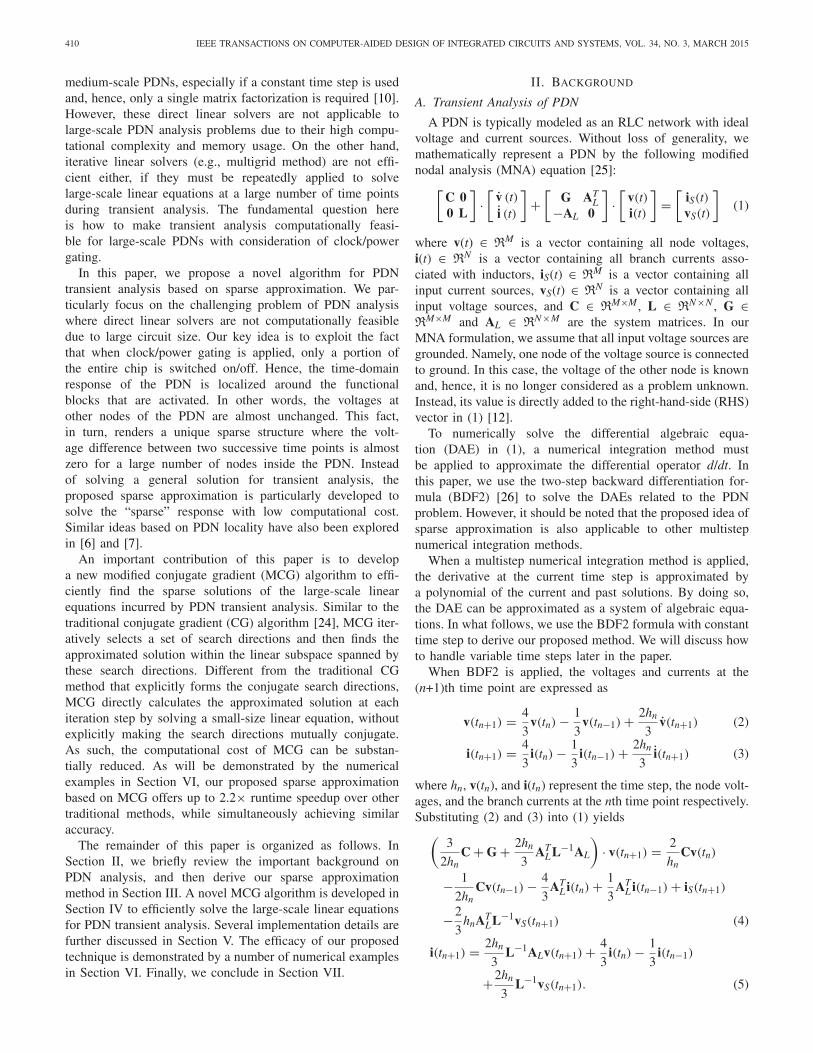
Fig. 1. Simple example illustrates the concept of localized transient responseassociated with clock/power gating. Only a small portion (black) of the chipis activated and the time-domain response of the PDN is localized within theblack and gray regions.

node voltages and branch currents. In this case, the incre-mental analysis problem for PDN can be formulated in thegeneral form of linear equation (6) where the unknown vec-tor x is sparse. Hence, instead of solving a general solution xfrom (6), we only need to decide the locations and values ofa few nonzeros.

Toward this goal, orthogonal matching pursuit (OMP) isapplied to solve the sparse solution x from the linear equationA·x = b [28]. OMP rewrites the RHS vector b as the linearcombination of all column vectors of the matrix A

b = x1a1 + x2a2 + · · · + xMaM (18)

where xm denotes the mth element of the vector x and am

stands for the mth column vector of the matrix A. Next,the “importance” of each column vector am is quantitativelyassessed by the normalized inner product

ρ(am, b) =∣∣∣∣ aT

mbaT

mam

∣∣∣∣. (19)

Intuitively, if ρ(am, b) is large, the column vector am playsan important role to represent the RHS vector b. Hence,the corresponding element xm should be nonzero. OMP iter-atively calculates the normalized inner products to selectthe nonzero elements from the vector x and then decidetheir values by finding the least-squares solution of an over-determined linear equation. Algorithm 2 summarizes the majorsteps of OMP.

III. TRANSIENT ANALYSIS BY SPARSE APPROXIMATION

In this paper, we further extend the idea of sparse approxi-mation from DC analysis to transient analysis. Our proposedapproach is motivated by the fact that when clock/power gatingis applied, only a small portion of the entire chip is activated.In this case, the transient response of the PDN is localizedin a small region. Namely, most node voltages and branchcurrents are almost constant between two consecutive timepoints. Fig. 1 shows a simple PDN example that conceptuallyillustrates the aforementioned concept of localized transientresponse.

Based on this observation, if we formulate the PDN equationwith respect to the incremental changes between two suc-cessive time points, the unknown solution vector containingthe incremental voltage changes is sparse. To derive such an

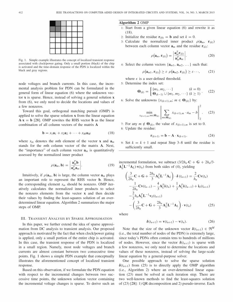
Algorithm 2 OMP1: Start from a given linear equation (6) and rewrite it as

(18).2: Initialize the residue r(0) = b and set k = 0.3: Calculate the normalized inner product ρ(am, r(k))

between each column vector am and the residue r(k):

ρ(am, r(k)

) =∣∣∣∣aT

mr(k)

aTmam

∣∣∣∣. (20)

4: Select the column vectors {am1, am2, . . . } such that:

ρ(am1, r(k)

) ≥ ε ρ(am2, r(k)

) ≥ ε · · ·, (21)

where ε is a user-defined threshold.5: Determine the index set:

�(k) ={ {m1, m2, · · · } (k = 0)

�(k−1) ∪ {m1, m2, · · · } (k ≥ 1). (22)

6: Solve the unknowns {x(k+1),m; m ∈ �(k)} by:

minx(k+1),m;m∈�(k)

∥∥∥∥∥∥∑

m∈�(k)

x(k+1),m · am − b

∥∥∥∥∥∥2

2

. (23)

7: For any m /∈ �(k), the value of x(k+1),m is set to 0.8: Update the residue:

r(k+1) = b − A · x(k+1). (24)

9: Set k = k + 1 and repeat Step 3–8 until the residue issufficiently small.

incremental formulation, we subtract (3/2hn·C + G + 2hn/3·AT

LL−1AL)·v(tn) from both sides of (4), yielding(3

2hnC + G + 2hn

3AT

LL−1AL

)· δ (tn+1) = 2

hnCv(tn)

− 1

2hnCv(tn−1) − 4

3AT

L i(tn) + 1

3AT

L i(tn−1) + iS(tn+1)

−2

3hnAT

LL−1vS(tn+1)

−(

3

2hnC + G + 2hn

3AT

LL−1AL

)· v(tn) (25)

where

δ(tn+1) = v(tn+1) − v(tn). (26)

Note that the size of the unknown vector δ(tn+1) ∈ RM

(i.e., the total number of nodes of the PDN) is extremely large,since today’s PDNs often contain tens to hundreds of millionsof nodes. However, since the vector δ(tn+1) is sparse witha few nonzeros, we only need to determine the locations andvalues of these nonzeros, instead of solving the large-scalelinear equation by a general-purpose solver.

One possible approach to solve the sparse solutionδ(tn+1) from (25) is to directly apply the OMP algorithm(i.e., Algorithm 2) where an over-determined linear equa-tion (23) must be solved at each iteration step. There aretwo well-known methods to find the least-squares solutionof (23) [28]: 1) QR decomposition and 2) pseudo-inverse. Each


method has its own advantages and limitations. QR decompo-sition is numerically stable, but computationally expensive. Onthe other hand, pseudo-inverse is computationally inexpensive,but often suffers from numerical issues. This lack of clearchoice motivates us to develop a highly efficient-yet-stablealgorithm, referred to as the MCG solver, to find the sparsesolution δ(tn+1) of (25) without solving any over-determinedlinear equation. The details of MCG will be discussed in thenext section.

IV. MCG SOLVER

Our proposed MCG solver is derived from the traditionalCG algorithm with several important modifications. First,MCG uses a different criterion to form the search directions.Second, it applies a different scheme to update the solutionby searching the linear subspace spanned by the search direc-tions. In this section, we derive the mathematical formulationof MCG in detail.

A. Mathematical Formulation

Without loss of generality, we consider the general repre-sentation of a linear equation A·x = b in (6). Our objective isto efficiently compute the sparse solution x. The incrementalformulation (25) can be easily mapped to this general formA·x = b by redefining the symbols

A = 3

2hnC + G + 2hn

3AT

LL−1AL (27)

x = δ (tn+1) (28)

b = 2

hnCv(tn) − 1

2hnCv(tn−1) − 4

3AT

L i(tn)

+ 1

3AT

L i(tn−1) + iS(tn+1) − 2

3hnAT

LL−1vS(tn+1)

−(

3

2hnC + G + 2hn

3AT

LL−1AL

)· v(tn). (29)

Note that the matrix A in (27) is symmetric and positivedefinite.

Since the unknown vector x contains a few nonzeros only,we propose to form the search directions based on the locationsof these nonzeros, instead of the residues used by the tradi-tional CG method (i.e., Algorithm 1). We use several heuristiccriteria to quantitatively assess the importance of each columnvector am of the matrix A, when calculating the incrementalresponse δ(tn+1) at the (n+1)th time point. As such, the cor-responding locations of the nonzeros in the unknown vectorδ(tn+1) can be quickly identified.

In particular, we develop two heuristic techniques. First, themth node is considered to be “active” and the correspondingincremental response δm(tn+1) [i.e., the mth element of theunknown vector δ(tn+1)] is expected to be nonzero, if at leastone of the following two conditions is satisfied.

1) The voltage of the mth node significantly varies at theprevious time point [i.e., the value of |δm(tn)| is large].

2) The mth node is connected to an input current or voltagesource (say, the ith current source iSi or voltage sourcevSi) that significantly varies at the current time point

[i.e., the value of |iSi(tn+1) − iSi(tn)| or |vSi(tn+1) −vSi(tn)| is large].

Note that the values of δm(tn), iSi(tn+1), iSi(tn), vSi(tn+1),and vSi(tn) are all known at the (n+1)th time point, whencalculating the incremental response δ(tn+1). Hence, thesetwo conditions can be easily checked. The indices of theseidentified nodes are used to form an initial index set �(0).

Second, in addition to the nodes that belong to the initialset �(0), a number of other nodes may also become activeat the (n+1)th time point, but are not captured by the afore-mentioned heuristics. For this reason, we further borrow theidea of normalized inner product in (20) to iteratively iden-tify these active nodes, similar to the OMP algorithm (i.e.,Algorithm 2). At the kth iteration step of the proposed MCGsolver, the indices of a set of activenodes (say, {m1, m2, . . . })are selected according to the normalized inner products andthese indices are cumulatively added to the index set �(k)

�(k) = �(k−1) ∪ {m1, m2, . . .}. (30)

Once the set �(k) is formed, we define the following searchdirections: {

em; m ∈ �(k)}

(31)

where em ∈ RM is a vector for which the mth element isone and all other elements are zero. When the vector em isselected as a search direction, it implies that the mth elementof the solution x of A·x = b, where A, x, and b are definedin (27)–(29), should be nonzero.

After the search directions are determined at the kth iterationstep, we form the following linear subspace:

�(k) = span{em; m ∈ �(k)

}. (32)

If the solution x is sparse and contains a few nonzeros only,it belongs to a low-dimensional linear subspace. In this case,MCG is able to accurately approximate the solution x withinvery few iteration steps. In other words, by exploiting the spar-sity of the solution x, MCG can converge more quickly thanthe traditional CG method.

Given the linear subspace �(k) at the kth iteration step of theMCG solver, we need to further determine the new solutionx(k+1) by solving the following optimization problem:

minx(k+1)∈�(k)

1

2xT(k+1)Ax(k+1) − bTx(k+1). (33)

The optimization problem in (33) is similar to that of thetraditional CG method shown in (12).

Note that the search directions in (31) are orthogonal butnot conjugate. Unlike the traditional CG method in which theconjugate search directions can be easily calculated from theresidues by (16), explicitly forming a set of conjugate searchdirections for the linear subspace in (32) is not trivial. While itis possible to make the vectors {em; m ∈ �(k)} conjugate byapplying Gram–Schmidt conjugation [24], such an approachcan be computationally prohibitive, especially for large-scaleproblems. Without explicitly knowing the conjugate searchdirections, the new solution x(k+1) cannot be calculated bydirectly following the simple equation expressed in (13).


To address this issue, we derive a new computing schemeto efficiently find the new solution x(k+1) from the linear sub-space �(k). Our proposed approach is based upon the propertyof orthogonality described by the following theorem.

Theorem 1: Given the solution x(k+1) solved by (12) wherethe initial value x(0) is 0 and the linear subspace �(k) is definedin (32), the residue r(k+1) = b − A·x(k+1) is orthogonal to allsearch directions {em; m ∈ �(k)}

eTmr(k+1) = 0

(m ∈ �(k)

). (34)

Proof: Since the solution x(k+1) is within the linear subspace�(k), it can be represented as the linear combination of allsearch directions

x(k+1) =∑

m∈�(k)

x(k+1),m · em. (35)

Hence, minimizing the cost function in (12) requires us tofind the values of {x(k+1),m; m ∈ �(k)} to satisfy the followingfirst-order optimality condition [29]:

∂

∂x(k+1),m

[1

2xT(k+1)Ax(k+1) − bTx(k+1)

]= 0

(m ∈ �(k)

).(36)

Substituting (35) into (36) yields

eTm · [

Ax(k+1) − b] = 0

(m ∈ �(k)

). (37)

Since the residue r(k+1) is equal to b − A·x(k+1),(37) implies the orthogonal property in (34). �

Assume that there are M(k) search directions {em; m ∈�(k)}, therefore M(k) nonzeros {x(k+1),m; m ∈ �(k)} areselected at the kth iteration step of the MCG algorithm.Namely, the cardinality (i.e., the size) of the set �(k) is M(k)∣∣�(k)

∣∣ = M(k). (38)

In this case, there are M(k) linear equations in (37) that wecan use to solve the M(k) unknowns {x(k+1),m; m ∈ �(k)}.In other words, the property of orthogonality described byTheorem 1 reveals a crucial fact that solving the optimizationproblem in (12) is equivalent to solving the linear equations in(37). This fact provides an alternative way to efficiently updatethe solution x(k+1) at the kth iteration step.

To further derive a compact representation of the reducedlinear equations in (37), we substitute (35) into (37)

eTm · A ·

∑m∈�(k)

x(k+1),m · em = eTmb

(m ∈ �(k)

). (39)

Equation (39) can be further rewritten as

ET�(k)AE�(k) · x�(k+1) = ET

�(k)b (40)

where E�(k) is an M-by-M(k) matrix containing the columnvectors {em; m ∈ �(k)} and x�(k+1) is an M(k)-by-one col-umn vector containing the unknowns {x(k+1),m; m ∈ �(k)}.Remember that em is a vector for which the mth elementis one and all other elements are zero. Hence, the reducedmatrix E�(k)

TAE�(k) in (40) is simply generated by select-ing the corresponding M(k) rows and columns from the matrixA. Namely, the matrix ET

�(k)AE�(k) is a principal minor [30]of the matrix A. Similarly, the reduced RHS vector ET

�(k)b in

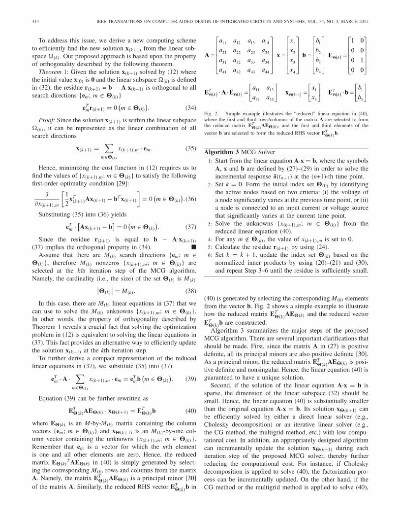
Fig. 2. Simple example illustrates the “reduced” linear equation in (40),where the first and third rows/columns of the matrix A are selected to formthe reduced matrix ET

�(k)AE�(k), and the first and third elements of the

vector b are selected to form the reduced RHS vector ET�(k)b.

Algorithm 3 MCG Solver1: Start from the linear equation A·x = b, where the symbols

A, x and b are defined by (27)–(29) in order to solve theincremental response δ(tn+1) at the (n+1)-th time point.

2: Set k = 0. Form the initial index set �(0) by identifyingthe active nodes based on two criteria: (i) the voltage ofa node significantly varies at the previous time point, or (ii)a node is connected to an input current or voltage sourcethat significantly varies at the current time point.

3: Solve the unknowns {x(k+1),m; m ∈ �(k)} from thereduced linear equation (40).

4: For any m /∈ �(k), the value of x(k+1),m is set to 0.5: Calculate the residue r(k+1) by using (24).6: Set k = k + 1, update the index set �(k) based on the

normalized inner products by using (20)–(21) and (30),and repeat Step 3–6 until the residue is sufficiently small.

(40) is generated by selecting the corresponding M(k) elementsfrom the vector b. Fig. 2 shows a simple example to illustratehow the reduced matrix ET

�(k)AE�(k) and the reduced vectorET

�(k)b are constructed.Algorithm 3 summarizes the major steps of the proposed

MCG algorithm. There are several important clarifications thatshould be made. First, since the matrix A in (27) is positivedefinite, all its principal minors are also positive definite [30].As a principal minor, the reduced matrix ET

�(k)AE�(k) is posi-tive definite and nonsingular. Hence, the linear equation (40) isguaranteed to have a unique solution.

Second, if the solution of the linear equation A·x = b issparse, the dimension of the linear subspace (32) should besmall. Hence, the linear equation (40) is substantially smallerthan the original equation A·x = b. Its solution x�(k+1) canbe efficiently solved by either a direct linear solver (e.g.,Cholesky decomposition) or an iterative linear solver (e.g.,the CG method, the multigrid method, etc.) with low compu-tational cost. In addition, an appropriately designed algorithmcan incrementally update the solution x�(k+1) during eachiteration step of the proposed MCG solver, thereby furtherreducing the computational cost. For instance, if Choleskydecomposition is applied to solve (40), the factorization pro-cess can be incrementally updated. On the other hand, if theCG method or the multigrid method is applied to solve (40),


the solution x�(k) from the previous iteration step can be usedto define an initial guess for the solution x�(k+1) of the cur-rent iteration step so that the iterative linear solver convergesquickly. Implementing such an incremental update schemeis straightforward and, therefore, the details are not furtherdiscussed in this paper.

B. Comparison With Traditional Sparse Solver

Our proposed MCG algorithm (i.e., Algorithm 3) is similarto the traditional OMP algorithm (i.e., Algorithm 2), becauseboth algorithms apply the same heuristics to iteratively iden-tify the nonzeros for the unknown solution vector based onnormalized inner product. However, once the nonzero loca-tions are determined and stored in the index set �(k) at thekth iteration step, MCG and OMP rely on different algorithmsto calculate the values of these nonzeros {x(k+1),m; m ∈ �(k)}.As shown in (23), OMP aims to find the least-squares solu-tion by minimizing the total squared error. The optimizationproblem in (23) can be rewritten as

minx(k+1)∈�(k)

1

2xT(k+1)A

TAx(k+1) − bTAx(k+1) (41)

where �(k) denotes the linear subspace defined in (32). On theother hand, MCG formulates a different optimization (33) tofind the solution x(k+1).

There are two consequences from the differences betweenthese two optimization formulations. First, the solutions from(33) and (41) are different if the solution of A·x = b doesnot exactly lie in the subspace �(k). As proven by Theorem 1,the MCG solution of (33) leads to a residue r(k+1) that isorthogonal to all search directions {em; m ∈ �(k)}. On theother hand, based on the theory of least-squares fitting [30],the OMP residue r(k+1) from (41) should be orthogonal to thecolumn vectors {am; m ∈ �(k)}

aTmr(k+1) = 0

(m ∈ �(k)

). (42)

Recall that em is a vector for which the mth element is oneand all other elements are zero. Hence, the following equalityholds:

Aem = am (m = 1, 2, . . . , M). (43)

Substituting (43) into (42) yields

eTmAr(k+1) = 0

(m ∈ �(k)

). (44)

It implies that the OMP residue r(k+1) and all searchdirections {em; m ∈ �(k)} are conjugate but not orthogonal.

Second and more importantly, the computational costsof solving (33) and (41) are different. As discussed inSection IV-A, solving (33) at each MCG iteration step isequivalent to solving a reduced linear equation (40). In thiscase, either Cholesky decomposition or the CG method can beapplied, because the linear equation (40) is positive definite.On the other hand, the least-squares solution of (41) can becomputed by either a direct linear solver (e.g., QR decomposi-tion) or an iterative linear solver (e.g., LSQR [31]). However,the least-squares solver is more expensive than a positive defi-nite linear equation solver, especially for large-scale problems.

Due to this reason, the proposed MCG algorithm is expectedto offer superior runtime efficiency over the traditional OMPmethod, as will be demonstrated by our numerical examplesin Section VI.

V. IMPLEMENTATION DETAILS

Our proposed PDN transient analysis based on sparseapproximation is made efficient by carefully addressing a num-ber of implementation issues. In this section, we discussthese implementation details and then summarize the overalltransient analysis flow.

A. Linear Solver Selection

As previously mentioned, the proposed MCG algorithmneeds to solve the linear equation (40) at each iteration step,as shown by Step 3 of Algorithm 3. Ideally, if the incrementalresponse δ(tn+1) in (25) is sparse, (40) is small and it can beefficiently solved by a direct linear solver based on Choleskydecomposition. However, if the incremental response δ(tn+1)is not sparse at a particular time point tn, a large linear equa-tion must be solved. In this case, directly applying Choleskydecomposition to solve (40) is not computationally efficient,since the computational complexity of Cholesky decomposi-tion grows quickly with the problem size. On the other hand,an iterative algebraic multigrid (AMG) solver [14] can beextremely efficient for large-scale equations; however, AMGis not as efficient as Cholesky decomposition for small-sizeproblems due to the overhead of constructing the interpolationand restriction operators [14].

To address this issue, we propose to adaptively select theappropriate linear solver based on the size of (40). If theequation size is sufficiently small (say, less than 0.5 × 106),Cholesky decomposition is used to solve (40). Otherwise, ifthe equation size is large (say, greater than 0.5×106), an AMGsolver is applied to find the solution of (40). Such an adaptivestrategy for solver selection allows us to fully take advantageof the trade-offs between computational efficiency and prob-lem size for different linear solvers in order to reduce theoverall runtime for a broad range of PDN analysis problems.

The aforementioned strategy of linear solver selection ismainly driven by computational cost. On the other hand, theaccuracy of these linear solvers is equally important and mustbe carefully considered. In particular, AMG is an iterativealgorithm and its error tolerance must be set to be suffi-ciently small due to the following two reasons. First, the AMGerror directly impacts the convergence of Algorithm 3. If theAMG solver is not sufficiently accurate, the residue calcu-lated by Step 5 of Algorithm 3 may be large, even if a lot ofactive nodes are selected. Second, the AMG error also playsan important role in estimating the LTE. Without an accu-rate AMG solver, LTE cannot be accurately calculated and,consequently, the time step for transient analysis cannot beappropriately determined, as will be discussed in detail in thenext subsection.

B. Adaptive Time Step Control

The LTE of a numerical integration method is stronglyaffected by the time step size. In many practical applications,


the time step has to be adjusted to ensure that the LTE is lessthan a predefined threshold. On the other hand, the time stepshould also be increased to speed up the transient simulationwhen the circuit behavior is relatively quiet. Although we cancontinuously adjust the time step based on the BDF2 formula,such an implementation can be computationally expensive andunnecessary. Instead, we implement a simple control schemewith discrete time step in this paper.

In particular, if the estimated LTE is too large, we reducethe time step by a factor of the power of two (i.e., 2, 4, 8,etc.). Otherwise, if the LTE is too small, we double the timestep. Because the BDF2 formula in (2) and (3) requires thesolutions at two past time points with the same time step, weuse an interpolation scheme to compute the solutions at themissing time points whenever the time step changes.

More specifically, assume that transient simulation is pro-gressing with the time step h from the time point tn−2 to tn−1and then from tn−1 to tn. At the time point tn, if the LTEestimation indicates that the LTE is greater than a predefinedthreshold, we need to reduce the time step and recalculate thesolution at tn. Instead of adopting a continuous time step thatmay be only slightly smaller than h, we reduce the time stepto h/2 (or even h/4 if necessary). After that, we interpolate thenode voltages v(tn−3/2) and the branch currents i(tn−3/2) at themiddle of tn−2 and tn−1 (denoted as tn−3/2). Since the timesteps tn−1 − tn−3/2 and tn − tn−1 are now both equal to h/2,we can proceed to use the BDF2 formula with constant timestep in (2) and (3) to continue our transient simulation. On theother hand, when the time step increases to 2h, we only needto select a few past solutions to make the equivalent time stepequal to 2h so that the BDF2 formula in (2) and (3) can againbe applied.

Given the aforementioned setup, the LTE of a capacitor volt-age or inductor current x at the nth time point can be estimatedby [32]

LTEx (tn) = h2n (hn + hn−1)

2

2hn + hn−1×〈x (tn) , x (tn−1) , x (tn−2) , x (tn−3)〉 (45)

where the operator <x(tn), x(tn−1), x(tn−2), x(tn−3)> is recur-sively defined as

〈x (tn) , x (tn−1) , · · · , x (tn−i)〉=

{x (tn) (i = 0)〈x(tn),··· ,x(tn−i+1)〉−〈x(tn−1),··· ,x(tn−i)〉

hn+hn−1+···+hn−i+1(i ≥ 1)

. (46)

For a given PDN containing RLC elements, the LTE valuesare calculated by (45) for all capacitor voltages and inductorcurrents and compared against the predefined threshold foradaptive time step control.

C. Summary

Algorithm 4 summarizes the major steps of the proposedtransient analysis algorithm for PDN. Before the transientanalysis starts, a DC analysis is first performed to deter-mine the initial condition of all node voltages and branchcurrents. Since, we focus on large-scale PDN analysis prob-lems that cannot be efficiently solved by a direct linear solver,

Algorithm 4 Transient Analysis for PDN1: Start from a given PDN that is described by (1) and the

time interval [0, tSTOP] for transient analysis.2: Derive the incremental formulation (25).3: Set an initial index n = 0, an initial time point t0 = 0,

and an initial time step h0 specified by the user.4: Apply a DC analysis to solve the initial node voltages

v(t0) and the initial branch currents i(t0).5: Set tn+1 = tn + hn, and solve the incremental response

δ(tn+1) by the MCG solver (i.e., Algorithm 3).6: Calculate the node voltages v(tn+1) by (26), and then the

branch currents i(tn+1) by (5).7: Calculate the LTE values for all capacitor voltages and

inductor currents by (45).8: If all LTE values are less than a user-defined threshold

(say, LTELOW ), set hn+1 = 2 · hn.9: If at least one of these LTE values is greater than a user-

defined threshold (say, LTEUP), set hn+1 = hn/2 and goto Step 5.

10: Set n = n + 1. Repeat Step 5–10 until tn reaches tSTOP.

the DC analysis in Step 4 of Algorithm 4 is implemented withan AMG solver [14]. Next, our proposed MCG solver (i.e.,Algorithm 3) is used to solve the linear equation (25) at eachtime point. As mentioned in Section V-A, Cholesky decom-position and AMG solver are adaptively selected to solve thelinear equation (40) at Step 3 of Algorithm 3. Finally, once thePDN response is known at the current time point, LTE valuesare calculated to adaptively adjust the time step, as discussedin Section V-B.

The runtime of the MCG solver at each time point dom-inates the overall computational time for transient analysis.Since MCG solves the reduced linear equation in (40) at eachiteration step (i.e., Step 3 of Algorithm 3), its computationalcomplexity can be expressed as O(Mα

(k)), where M(k) denotesthe number of unknowns of the reduced linear equation atthe kth iteration step and the constant α is usually between 1and 2. For many practical problems, the incremental responsedefined by (26) is sparse and contains few nonzeros. Hence,M(k) is much less than the total number of nodes of the PDN(i.e., M). For this reason, our proposed MCG solver is compu-tationally more efficient than the traditional linear solver forwhich the computational complexity is O(Mα).

VI. NUMERICAL EXAMPLES

A. Experimental Setup

In this section, we demonstrate the efficacy of our proposedPDN transient analysis for six large-scale circuit examples, asshown in Table I. These six test cases, labeled as PND1–PDN6 in Table I, are from the IBM benchmarks ibmpg3-ibmpg6, ibmpgnew1, and ibmpgnew2 given in [33]. In thispaper, the two benchmarks ibmpg1 and ibmpg2 are excluded,since their circuit sizes are small and, hence, they are not con-sidered as good examples to validate our proposed algorithmthat is particularly developed for large-scale circuits.


TABLE IPDN BENCHMARK INFORMATION

To emulate the effect of clock/power gating, we simultane-ously turn on/off all current sources within a local region thatis defined by a bounding box. The percentage of the currentsources being activated or deactivated is referred to the acti-vation rate in this paper. In our experiment, the size of thebounding box is appropriately set so that the activation rateis around 10% for each benchmark circuit. The waveform ofeach current source is set to a step function in time domainwhere the rising time equals 0.1 ns.

For testing and comparison purposes, three different tech-niques are implemented for PDN transient analysis. All thesethree implementations use the BDF2 formula [26] for numer-ical integration with adaptive time step control. The onlydifference between them lies in the linear solver that is used tosolve the linear equation (25) at each time point: 1) the AMGsolver [14]; 2) the OMP solver [28]; and 3) the proposed MCGsolver.

To measure and compare the accuracy for different tech-niques, a “golden” linear solver is further implemented togenerate the golden solution for each test case. The goldensolver applies the BDF2 formula [26] for numerical integra-tion with a fixed time step that is sufficiently small and,hence, the LTE of the golden solver is negligible. In addi-tion, the golden solver uses Cholesky decomposition to solvethe linear equation (25) at each time point. Hence, theresulting residue of (25) is also negligible for the goldensolver.

It is important to emphasize that the computationalcomplexity of Cholesky decomposition grows quickly withproblem size. Even though, Cholesky decomposition remainsfeasible for all test cases shown in Table I, it would quicklybecome computationally infeasible as circuit size furtherincreases. In this paper, the proposed MCG algorithm is partic-ularly developed to handle large-scale PDN analysis problemswhere direct linear solvers are not computationally feasible.Here, we only use a number of medium-scale PDN examplesto validate the MCG algorithm, because we need to applyCholesky decomposition to calculate the golden solution foraccuracy comparison.

For all test cases, the transient analysis is performed overthe time interval [0, 100 ns]. The time interval is set to besufficiently long for the transient response to die out. Allexperiments are executed on a Linux server with Intel Xeon2.67 GHz CPU and 512 GB memory.

B. Comparison on Accuracy and Speed

Table II shows the computational time, memory consump-tion, and simulation error for three different implementations.

TABLE IICOMPARISON ON ACCURACY AND RUNTIME FOR TRANSIENT

ANALYSIS OF PDNS (ACTIVATION RATE ≈ 10%)

Here, the mean and maximum errors are respectivelydefined as

ErrorMean = 1

M· 1

tSTOP·

M∑m=1

∫ tSTOP

0|vm(t) − vm(t)| · dt

≈ 1

M· 1

tSTOP·

M∑m=1

N∑n=0

|vm(tn+1) − vm(tn+1)| · hn

(47)

ErrorMax = maxm,n

|vm (tn) − vm (tn)| (48)

where vm(t) and vm(t) denote the exact and estimated nodevoltages at the time t respectively, tSTOP represents the upperbound of the time interval for transient analysis, and hn standsfor the time step at the nth time point.

Studying Table II, we notice that the OMP solver canbe computationally expensive for a number of benchmarks.Taking PDN1 as an example, we observe from our experimentthat the least-squares problem in (23) is ill-conditioned. In ourimplementation of OMP, the least-squares solution of (23) iscomputed by pseudo-inverse, instead of QR decomposition,in order to minimize the computational cost. Therefore, OMPcannot accurately find the least-squares solution for PDN1 andthe OMP solver eventually has to use AMG to solve the full-size linear equation at almost all time points. It, in turn, resultsin expensive computational cost.

In addition, the numerical issue of OMP can further impactthe LTE estimation during transient analysis. ConsideringPDN2 as an example, we observe from Table II that OMPtakes significantly more time steps than AMG and MCG tofinish the transient analysis, thereby resulting in expensivecomputational cost. Such an observation is made, because theOMP solver is not numerically robust and its solution is nothighly accurate. Therefore, the LTE is not accurately estimatedand the transient analysis fails to use the appropriate time stepto perform numerical integration in this example.


Fig. 3. Time step sizes of MCG are plotted at different time points forPDN6.

AMG and MCG, on the other hand, work perfectly withthe adaptive time step control based on LTE. The numbers oftime steps associated with AMG and MCG are almost iden-tical, as shown in Table II. To further validate the time stepcontrol scheme for MCG, we closely examine the time stepsizes during transient analysis. Since the rising time of theinput current sources is set to 0.1 ns, the initial time step sizeis chosen as 10 ps for all benchmarks. As the time evolvesand the transient response dies out, the time step sizes areadaptively increased to larger values (e.g., more than 10 ns atthe end of the transient analysis). The average time step sizeover all six benchmarks is equal to 1.7 ns. Taking PDN6 asan example, Fig. 3 shows its time step sizes at different timepoints where the time step size gradually increases over time.

Compared to AMG, MCG reduces the runtime by up to2.2×, while simultaneously achieving similar accuracy, asshown in Table II. In particular, the maximum error is almostidentical for AMG and MCG over all benchmarks. Note thatthe maximum error is often of greater importance than themean error for many practical applications, since we wantto predict the worst-case voltage droop, instead of the aver-age voltage droop, by running transient simulation. For thesetest cases, MCG demonstrates superior performance, becauseit efficiently exploits the sparse property of the incremen-tal response δ(tn+1), while AMG is a general-purpose linearsolver and is not particularly tuned to solve sparse solutions.

The memory usages of AMG, OMP, and MCG are measuredat each time step by counting the size of the major data struc-tures, as shown in Table II. Note that OMP and MCG consumeless memory than AMG. Such an observation is made, becauseOMP and MCG only need to solve a reduced linear equationwith reduced memory consumption, when the circuit responseis sparse.

C. Visualization of Results

In this subsection, we take the benchmark PDN6 as anexample to show several important findings related to the pro-posed transient analysis based on sparse approximation. Thesestudies provide a number of intuitive insights about our pro-posed method, thereby facilitating us to further understand itsadvantages and limitations.

Fig. 4. Golden PDN response is calculated by transient analysis implementedwith a direct linear solver and is plotted for two selected nodes of PDN6.(a) One node within the activated region. (b) One node outside the activatedregion.

Fig. 5. Golden incremental voltage response δ(t) is solved from (25) and(26) by a direct linear solver and its histogram is plotted at two selectedtime points for PDN6. (a) t = 3 ns at the beginning of the transient analysis.(b) t = 100 ns at the end of the transient analysis.

Fig. 4 shows the transient response of two selected nodesfrom PDN6. One is inside the activated region, and the otheris outside the activated region. A large-scale oscillation isobserved for the voltage response associated with the nodeinside the activated region, due to the underdamped natureof the PDN. On the other hand, the voltage response isalmost constant over time for the node outside the activatedregion, as is expected. In this case, the incremental voltageresponse associated with the inactive node is almost zero. It, inturn, facilitates our proposed sparse approximation to achieveextremely high efficiency for transient analysis.

Fig. 5 plots the incremental voltage response δ(t) at two dif-ferent time points: 1) t = 3 ns at the beginning of the transientanalysis and 2) t = 100 ns at the end of the transient anal-ysis. Two important observations can be made from Fig. 5.First, since a small portion of current sources are turned on,only a small number of nodes are activated in this example.Hence, the incremental voltage response δ(t) is close to zerofor most nodes at the beginning of the transient analysis, asshown in Fig. 5(a). Second, but more importantly, as the tran-sient response dies out at the end of the transient analysis, theincremental voltage response δ(t) becomes almost zero for allnodes at t = 100 ns. In this case, since the vector δ(t) containsfew nonzeros, it can be efficiently determined by the proposedMCG solver with low computational cost.

Figs. 6 and 7 further plot the incremental voltage responseδ(t) as a function of the spatial location for different layers(one bottom layer and one top layer) at t = 3 ns and t = 100 ns,respectively. Studying Figs. 6 and 7 reveals an important factthat the incremental response δ(t) is close to zero for a largenumber of nodes at t = 3 ns and it becomes almost zero for


Fig. 6. Golden incremental voltage response δ(tn) is solved from (25) and(26) by a direct linear solver and |δ(tn)| is plotted for two selected metal layersof PDN6 at t = 3 ns. (a) Bottom metal layer (b) Top metal layer. The colorindicates the magnitude of |δ(tn)| with the unit of mV.

Fig. 7. Golden incremental voltage response δ(tn) is solved from (25) and(26) by a direct linear solver and |δ(tn)| is plotted for two selected metal layersof PDN6 at t = 100 ns. (a) Bottom metal layer (b) Top metal layer. The colorindicates the magnitude of |δ(tn)| with the unit of mV.

Fig. 8. Histogram of the percentage of occurrence is plotted for transientsimulation of PDN6 by using MCG.

all nodes at t = 100 ns. This observation is consistent withthat shown in Fig. 5.

Fig. 8 shows the histogram of the percentage of occurrencefor each node being selected by the MCG solver during tran-sient simulation. Here, the occurrence of a node is defined asthe number of time points for the node being selected, and thepercentage of occurrence of a node is defined as the ratio ofits occurrence over the total number of time points. In otherwords, if the percentage of occurrence is high for a particularnode, this node is considered to be active at most time points.As shown in Fig. 8, for more than half of the nodes, the per-centage of occurrence is less than 60%, implying that a largenumber of nodes are “inactive” and the corresponding incre-mental response is zero at many time points. This is additionalevidence to explain the reason why the proposed transient

TABLE IIICOMPARISON ON ACCURACY AND RUNTIME FOR TRANSIENT ANALYSIS

OF PDN6 BY VARYING ACTIVATION RATE

Fig. 9. Runtime speed-up of MCG over AMG and the percentage of selectednodes by MCG are plotted as functions of the activation rate for PDN6.

analysis based on sparse approximation is computationallyefficient.

D. Impact of Activation Rate

In this subsection, we further study the efficiency of MCGby varying the activation rate. Similar to the previous sub-section, we again take the benchmark PDN6 as an example.Table III compares the runtime and error for two differentsolvers: 1) AMG and 2) MCG. Here, we do not include theOMP results, because the OMP solver suffers from numericalissues, as is demonstrated in Section VI-B.

To clearly explain the impact of activation rate, Fig. 9 plotsthe runtime speed-up of MCG over AMG and the percentageof selected nodes by MCG as functions of the activation rate.Here, the percentage of selected nodes is equal to the averagenumber of selected nodes over all time points divided by thetotal number of circuit nodes.

Several important observations can be made from the data inTable III and Fig. 9. First, as the activation rate increases,the number of time steps increases for both AMG andMCG. Intuitively, as more circuit components become active,a smaller time step must be used to perform transient analysis.Second, the runtime of both AMG and MCG increases with the


activation rate. The runtime of AMG increases, mostly becausethe number of time steps increases. On the other hand, the run-time of MCG increases due to two reasons: 1) the increase ofthe number of time steps as shown in Table III and 2) theincrease of the number of active nodes selected by MCG asshown in Fig. 9.

Finally, the runtime speed-up of MCG over AMG decreaseswith the activation rate, as the sparsity of the solution isreduced. However, MCG is still more computationally efficientthan AMG (i.e., less computational time but similar simula-tion accuracy), even if the activation rate is as large as 50%.Note that the maximum error is almost identical for AMG andMCG over all cases in Table III.

VII. CONCLUSION

In this paper, an efficient method based on sparse approxi-mation is proposed for transient analysis of large-scale PDNs.By exploiting the unique sparse structure of the transientresponse of PDNs with clock/power gating, an MCG algorithmis developed to efficiently find the sparse solution (i.e., theincremental voltage response of the PDN) of a linear, positivedefinite equation. The MCG algorithm facilitates the proposedtransient analysis to reduce runtime over other general-purposelinear solvers. As being demonstrated by the numerical exam-ples in this paper, the proposed transient analysis based onsparse approximation offers up to 2.2× speedup over othertraditional methods, while achieving similar accuracy.

The proposed MCG solver is computationally efficient ifthe solution vector is sparse. If the solution is not sparse,a traditional linear solver (i.e., either a direct linear solveror an iterative linear solver) is preferred. In practice, a heuris-tic scheme for sparsity detection can be possibly incorporatedinto the MCG algorithm. More specifically, if a large num-ber of active nodes are detected within the iteration loop ofAlgorithm 3, we should abort the MCG solver and switch tothe traditional linear solver. The detailed implementation ofthe aforementioned heuristics for sparsity detection is beyondthe scope of this paper and will be further studied in our futureresearch.

It is worth mentioning that the large overhead ofclock/power gating often prevents today’s IC designers fromusing a large number of clock/power domains. However,the advance of several emerging technologies (e.g., on-chipDC-DC converter [34] and 3-D integration [35]) has broughtup several new opportunities to explore the feasibility of usingfine-grain clock/power domains for future ICs [36]. Due tothis reason, the efficacy of the proposed MCG algorithm isexpected to be more pronounced for simulating future PDNs.

Finally, it is important to note that the proposed idea ofsparse approximation is not limited to linear circuits (e.g.,PDNs) only. It can be further extended to transient analysis ofnonlinear circuits, such as logic circuits and SRAM circuits,where the transient response is localized in a small region anda large portion of the circuit is inactive. In these cases, a num-ber of linear equations must be repeatedly solved during theNewton–Raphson iteration [25]. Since the Jacobian matrix ofa general nonlinear circuit may not be symmetric and positive

definite, a different iterative algorithm such as the general-ized minimal residual (GMRES) method [37], instead of theCG method, must be used to construct the sparse linear solver.More details along this direction are not included in this paperbut will be studied in our future research.

REFERENCES

[1] S. Nassif and J. Kozhaya, “Fast power grid simulation,” in Proc. DesignAutom. Conf., Los Angeles, CA, USA, 2000, pp. 156–161.

[2] S. Nassif, “Power grid analysis benchmarks,” in Proc. Asia South Pac.Design Autom. Conf., Seoul, Korea, 2008, pp. 376–381.

[3] Q. Zhu, Power Distribution Network Design for VLSI. Hoboken, NJ,USA: Wiley, 2004.

[4] P. Ghanta, S. Vrudhula, R. Panda, and J. Wang, “Stochastic power gridanalysis considering process variations,” in Proc. Design Autom. TestEur., vol. 2. Munich, Germany, 2005, pp. 964–969.

[5] S. Pant, D. Blaauw, V. Zolotov, S. Sundareswaran, and R. Panda,“A stochastic approach to power grid analysis,” in Proc. Design Autom.Conf., San Francisco, CA, USA, 2004, pp. 171–176.

[6] E. Chiprout, “Fast flip-chip power grid analysis via locality and gridshells,” in Proc. Int. Conf. Comput.-Aided Design, San Jose, CA, USA,2004, pp. 485–488.

[7] S. Pant and E. Chiprout, “Power grid physics and implications forCAD,” in Proc. Design Autom. Conf., San Francisco, CA, USA, 2006,pp. 199–204.

[8] R. Mandrekar, K. Srinivasan, E. Engin, and M. Swminathan, “Causalityenforcement in transient co-simulation of signal and power deliverynetworks,” IEEE Trans. Adv. Packag., vol. 30, no. 2, pp. 270–278,May 2007.

[9] T. Chen and C. Chen, “Efficient large-scale power grid analysis basedon preconditioned Krylov-subspace iterative methods,” in Proc. DesignAutom. Conf., Las Vegas, NV, USA, 2001, pp. 559–562.

[10] S. Weng, Q. Chen, and C. Cheng, “Time-domain analysis of large-scale circuits by matrix exponential method with adaptive control,”IEEE Trans. Comput.-Aided Design Integr. Circuits Syst., vol. 31, no. 8,pp. 1180–1193, Aug. 2012.

[11] M. Zhao, R. Panda, S. Sapatnekar, and D. Blaauw, “Hierarchical analysisof power distribution networks,” IEEE Trans. Comput.-Aided DesignIntegr. Circuits Syst., vol. 21, no. 2, pp. 159–168, Feb. 2002.

[12] J. Yang, Z. Li, Y. Cai, and Q. Zhou, “PowerRush: An efficient simulatorfor static power grid analysis,” IEEE Trans. Very Large Scale Integr.(VLSI) Syst., vol. 22, no. 10, pp. 2103–2116, Oct. 2014.

[13] J. Kozhaya, S. Nassif, and F. Najm, “A multigrid-like technique forpower grid analysis,” IEEE Trans. Comput.-Aided Design Integr. CircuitsSyst., vol. 21, no. 10, pp. 1148–1160, Oct. 2002.

[14] H. Su, E. Acar, and S. Nassif, “Power grid reduction based on algebraicmultigrid principles,” in Proc. Design Autom. Conf., Anaheim, CA, USA,2003, pp. 109–112.

[15] Z. Feng and P. Li, “Multigrid on GPU: Tackling power grid analysison parallel SIMT platforms,” in Proc. Int. Conf. Comput.-Aided Design,San Jose, CA, USA, 2008, pp. 647–654.

[16] Z. Feng and Z. Zeng, “Parallel multigrid preconditioning on graphicsprocessing units (GPUs) for robust power grid analysis,” in Proc. DesignAutom. Conf., Anaheim, CA, USA, 2010, pp. 661–666.

[17] H. Qian, S. Nassif, and S. Sapatnekar, “Power grid analysis using ran-dom walks,” IEEE Trans. Comput.-Aided Design Integr. Circuits Syst.,vol. 24, no. 8, pp. 1204–1224, Aug. 2005.

[18] D. Kouroussis and F. Najm, “A static pattern-independent technique forpower grid voltage integrity verification,” in Proc. Design Autom. Conf.,Anaheim, CA, USA, 2003, pp. 99–104.

[19] H. Qian, S. Nassif, and S. Sapatnekar, “Early-stage power grid analy-sis for uncertain working modes,” IEEE Trans. Comput.-Aided DesignIntegr. Circuits Syst., vol. 24, no. 5, pp. 676–682, May 2005.

[20] X. Xiong and J. Wang, “Vectorless verification of RLC power grids withtransient current constraints,” in Proc. Int. Conf. Comput.-Aided Design,San Jose, CA, USA, 2011, pp. 548–554.

[21] Q. Wu, M. Pedram, and X. Wu, “Clock-gating and its application tolow power design of sequential circuits,” IEEE Trans. Circuits Syst. I,Fundam. Theory Appl., vol. 47, no. 3, pp. 415–420, Mar. 2000.

[22] K. Agarwal, K. Nowka, H. Deogun, and D. Sylvester, “Power gatingwith multiple sleep modes,” in Proc. Int. Symp. Qual. Electron. Design,San Jose, CA, USA, 2006, pp. 633–637.


[23] W. Zhang et al., “Efficient power network analysis considering multido-main clock gating,” IEEE Trans. Comput.-Aided Design Integr. CircuitsSyst., vol. 28, no. 9, pp. 1348–1358, Jan. 2009.

[24] J. Shewchuk. (Aug. 1994). An Introduction to the ConjugateGradient Method Without the Agonizing Pain. [Online]. Available:http://www.cs.cmu.edu/∼quake-papers/ painless-conjugate-gradient.pdf

[25] L. Pillage, R. A. Rohrer, and C. Visweswariah, Electronic Circuit andSystem Simulation Methods. New York, NY, USA: McGraw-Hill, 1998.

[26] C. Gear, “Simultaneous numerical solution of differential-algebraicequations,” IEEE Trans. Circuit Theory, vol. 18, no. 1, pp. 89–95,Jan. 1971.

[27] A. Devgan, H. Ji, and W. Dai, “How to efficiently capture on-chip induc-tance effects: Introducing a new circuit element K,” in Proc. Int. Conf.Comput.-Aided Design, San Jose, CA, USA, 2000, pp. 150–155.

[28] P. Sun, X. Li, and M. Ting, “Efficient incremental analysis of on-chippower grid via sparse approximation,” in Proc. Design Autom. Conf.,San Francisco, CA, USA, 2011, pp. 676–681.

[29] D. Bertsekas, Nonlinear Programming. Belmont, MA, USA:Athena Scientific, 1999.

[30] R. Horn and C. Johnson, Matrix Analysis. Cambridge, U.K.: CambridgeUniv. Press, 1990.

[31] C. Paige and M. Saunders, “LSQR: An algorithm for sparse linear equa-tions and sparse least squares,” ACM Trans. Math. Softw., vol. 8, no. 1,pp. 43–71, Mar. 1982.

[32] J. Verner, “Explicit Runge-Kutta methods with estimates of the localtruncation error,” SIAM J. Numer. Anal., vol. 15, no. 4, pp. 772–790,Aug. 1978.

[33] Z. Li, P. Li, and S. Nassif. (Aug. 2011). IBM Power Grid Benchmarks.[Online]. Available: http://dropzone.tamu.edu/∼pli/PGBench/

[34] H. Le, S. Randers, and E. Alon, “Design techniques for fully integratedswitched-capacitor DC-DC converters,” IEEE J. Solid-State Circuits,vol. 48, no. 9, pp. 2120–2131, Sep. 2011.

[35] Y. Xie, J. Cong, and S. Sapatnekar, Three-Dimensional IC: Design, CAD,and Architecture. New York, NY, USA: Springer, 2009.

[36] H. Esmaeilzadeh, E. Blern, R. Amant, K. Sankaralingam, and D. Burger,“Dark silicon and the end of multicore scaling,” in Proc. Int. Symp.Comput. Archit., Portland, OR, USA, 2011, pp. 365–376.

[37] Y. Saad and M. Schultz, “GMRES: A generalized minimal residualalgorithm for solving nonsymmetric linear systems,” SIAM J. Sci. Stat.Comput., vol. 7, no. 3, pp. 856–869, Jul. 1986.

Hengliang Zhu (S’07–M’09) received the B.E.degree in electronic engineering from the Universityof Science and Technology of China, Hefei, China,and the Ph.D. degree in microelectronics from FudanUniversity, Shanghai, China, in 2004 and 2009,respectively.

He joined the State Key Laboratory of ASIC& System, Microelectronics Department, FudanUniversity, as an Assistant Professor, in 2009. Hiscurrent research interests include circuit analysis,interconnect parameter extraction, and model orderreduction.

Yuanzhe Wang received the B.Eng. and M.Phil.degrees in electrical engineering from TianjinUniversity, Tianjin, China, and the Universityof Hong Kong, Hong Kong, in 2009 and 2011,respectively.

He is currently with the Department of Electricaland Computer Engineering, Carnegie MellonUniversity, Pittsburgh, PA, USA. His currentresearch interests include self-healing of analogcircuits and power grid analysis.

Frank Liu (S’95–M’99–SM’09) received the M.S.degree in applied mathematics from the Universityof Minnesota, Minneapolis, MN, USA, and thePh.D. degree in electrical and computer engineeringfrom Carnegie Mellon University, Pittsburgh, PA,USA.

He is currently a Research Staff Member withIBM Austin Research Laboratory, Austin, TX,USA. He has authored and co-authored over 60 con-ference and journal papers.

Dr. Liu was the recipient of the Best PaperAward at Asian-Pacific Design Automation Conference, the IEEE DonaldO. Pederson Best Paper Award, and the Multiple IBM Research DivisionAccomplishment Awards. He was an ACM SIGDA Executive CommitteeMember from 2012 to 2015.

Xin Li (S’01–M’06–SM’10) received the B.S. andM.S. degrees in electronics engineering from FudanUniversity, Shanghai, China, in 1998 and 2001,respectively, and the Ph.D. degree in electricaland computer engineering from Carnegie MellonUniversity, Pittsburgh, PA, USA, in 2005.

He is currently an Associate Professor with theDepartment of Electrical and Computer Engineering,Carnegie Mellon University. His current researchinterests include computer-aided design, neuralsignal processing, and power system analysis

and design.Dr. Li was the recipient of the National Science Foundation Faculty

Early Career Development Award in 2012, the Best Paper Award fromDesign Automation Conference in 2010, and the IEEE/ACM WilliamJ. McCalla ICCAD Best Paper Awards twice in 2004 and 2011.

Xuan Zeng (M’97) received the B.S. and Ph.D.degrees in electrical engineering from FudanUniversity, Shanghai, China, in 1991 and 1997,respectively.

She is currently a Full Professor with theDepartment of Microelectronics, Fudan University,where she was the Director of the State KeyLaboratory of ASIC & System, from 2008 to 2012.She was a Visiting Professor at the Departmentof Electrical Engineering, Texas A&M University,College Station, TX, USA, and the Department of

Microelectronics, Technische Universiteit Delft, Delft, The Netherlands, in2002 and 2003, respectively. Her current research interests include design formanufacturability, high-speed interconnect analysis and optimization, analogbehavioral modeling, circuit simulation, and ASIC design.

Dr. Zeng was the recipient of the Chinese National Science Funds forDistinguished Young Scientists in 2011 and the First-Class of Natural SciencePrize of Shanghai in 2012. She is the Changjiang Distinguished Professor withthe Ministry of Education Department of China in 2014.

Peter Feldmann (F’00) was born in Timisoara,Romania. He received the B.Sc. degree (summa cumlaude) in computer engineering and the M.Sc. degreein electrical engineering, both from the Technion–Israel Institute of Technology, Haifa, Israel, in 1983and 1987, respectively, and the Ph.D. degree fromCarnegie Mellon University, Pittsburgh, PA, USA,in 1991.

He was a Designer in digital signal proces-sors at Zoran Microelectronics, Haifa. He wasa Distinguished Technical Staff Member at Design

Principles Research Department, Bell Laboratories, Murray Hill, NJ, USA,and also a Research Staff Member at the IBM T.J. Watson Research Center,Yorktown Heights, NY, USA. He is currently with D. E. Shaw Research,New York City, NY, USA, researching on hardware accelerated moleculardynamics simulation. He was the Vice President of the VLSI and IntegratedElectro-optics at CeLight, Silver Spring, MD, USA, a fiber-optic communi-cations start-up. He was an Adjunct Professor at the Columbia UniversityElectrical Engineering Department, New York. His current research interestsinclude analysis, modeling, design, and optimization methods for integratedelectronic circuits and communication systems, analysis and modeling fortiming, power, and noise in digital VLSI circuits, and also on the large-scaledynamic analysis and modeling of the electricity transmission grid. He hasauthored over hundred papers and patents.

ieee transactions on computer-aided …xinli/papers/2015_tcad_pg.pdfdigital object identiﬁer...

Documents