Imitation of a procedural greenhouse modelwith an artificial neural network

R. KOK, R. LACROIX, G. CLARK and E. TAILLEFER

Agricultural Engineering, Macdonald Campus of McGill University, 21111 Lakeshore Blvd., Ste. Anne de Bellevue, QC,Canada H9X 3V9. Received 4 August 1992; accepted 26 April 1994.

Kok, R., Lacroix, R., Clark, G. and Taillefer, E. 1994. Imitation ofa procedural greenhouse model with an artificial neural network. Can. Agric. Eng. 36:117-126. Our overall objective is toreplace procedural models with neural networks for some reasoningactivities in cognitive systems. We have initially attempted to imitatea procedural thermal exchange model of a greenhouse with a numberof neural networks, each of which was subjected to various amountsof learning. An evaluation method was developed with which theperformance of each network was compared to that of the proceduralmodel. The efficacy of the evaluation method was assessed in comparison to human visual judgment. Each network was also tested forits ability to respond meaningfully to data sets which were differentfrom its learning set. The evaluation method was found to agree withthe general trend of human visual judgment and can be used tomonitor a network's progress in learning. The networks were giveninput values for date, time, solar radiation, exterior temperature,relative humidity, and wind speed, as well as one-hour lag values ofthe radiation and exterior temperature. After 100,000 learning cycles, the networks adequately mimicked the greenhouse proceduralmodel with regard to the three output variables of interest: interiortemperature, heating load, and ventilation. This network configuration (8 inputs, 3 outputs, 100,000 learning cycles) also performedacceptably when the input data used during recall were differentfrom those used for learning.

Notre objectif global est de remplacer les modeles procedurauxpar des reseaux de neurones pour certaines activites de raisonnementdans les systemes cognitifs. Nous avons tente d'imiter un modeleprocedural des echanges thermiques en serre avec plusieurs reseauxneuroniques, ou chacun fut soumis a differents degres d'apprentis-sage. Pour juger la performance des divers reseaux, une methoded'evaluation a ete developpee et son efficacite a ete etablie encomparaison avec le jugement visuel humain. La capacite a reagircorrectement a des donnees provenant d'une serie autre que celleayant servi a 1'apprentissage a aussi ete testee a l'aide d'un reseauchoisi parmi I'ensemble. La methode d'evaluation a ete jugee commecorrespondant bien a la tendance generale du jugement visuel humain et peut etre utilisee poursuivre les progresdans 1'apprentissaged'un reseau neuronique. Pour le cas specifique etudie, apres 100,000cycles d'apprentissage, le reseau ayant comme entrees la date,1'heure, le rayonnement solaire, la temperature et I'humidite relativeexterieures et la vitesse du vent, ainsi que les valeurs de 1'heureprecedente pour le rayonnement solaire et la temperature exterieure,est celui qui a le mieux imite le comportement des trois variablesconsiderees: la temperature interieure, la demande de chauffage et lademande de ventilation. Cette configuration (8 entrees, 3 sorties,100,000 cycles) a aussi produit des resultats acceptables lorsque lerappel etait fait avec des entrees differentes de celles utilisees durant1'apprentissage.

INTRODUCTION

The design and assembly of enclosed agro-ecosystems(EAE's) is receiving increasing attention. Some applicationsof this technology have been discussed by Wilkins (1988),Johnson and Wetzel (1990), and Salisbury (1991). Theyrange from production greenhouses, phytotrons, and novelenvironments for humans (such as space-based farms), toentirely new life forms. The structure and sophistication of anEAE's control system determine the degree to which it isreliant on external authority for decision-making and how"deep" its own decision-making processes are (i.e., whatfactors are taken into account, what alternatives are considered, how optimized the decisions are, etc.). In the long termour interest lies in creating a fully autonomous, highly cognitive EAE. Presently our focus is on describing, specifyingand assembling a suitable control system. As part of itscognitive faculties, such a system might have a consciousness, which we conceive to be simulation based. That is, thesystem would assess the aptness and profitability of variousaction paths by means of models which would incorporaterepresentations of itself acting within its environment.

Until now our simulations have been based on proceduralmodels, but neural networks might be faster and more efficient in some situations. A neural network, like a proceduralmodel or rule-based expert system, is a manifestation of atransfer function which uses the values of input variables todetermine the values of output variables. In all three instances, the intent is to imitate the human capacity to expressa relationship. Neural networks, however, constitute an interesting alternative to the other methods mentioned. Afundamental difference between the neural approach and theothers is that neural computing is done with a structureresembling that of the human brain and central nervous system. A major advantage of this is that knowledge does notneed to be extracted from the incoming data, explicitly stated,and then separately encoded. Knowledge is instead embedded directly in the neural network, in the values of theconnections between the network nodes. It resides there in an

inherent and distributed fashion; data need not be forced intoa conceptual mould such as that manifested in the structureof a spreadsheet or database. This implicitness of knowledgecan also be viewed as a disadvantage, because it is difficultto transfer the information to other platforms; it is impossibleto know the extent of a network's "knowledge" except via itsbehaviour. A neural network's internalization of knowledge(learning) takes place gradually and is not limited to a single

CANADIAN AGRICULTURAL ENGINEERING Vol. 36, No. 2. April/May/June 1994 117

extraction phase. Instead, the neural net can be made tocontinue to learn and evolve each time it receives a new setof input data.

In a formal rule-based expert system, knowledge is encoded explicitly in sets of rules. To construct an expertsystem, the rules must be individually extracted from domainspecialists, who are confined to a tight conceptual framework. Next, the rules must be explicitly expressed in astandard form, such as the IF..THEN construct, and these statements are then added to a rule base. During consultation, thechaining between the rules is managed by an inference engine.Any differences between the behaviour of the real system andthat simulated by the expert system must be resolved by reworking some or all of the steps discussed above.

The creation of a procedural model is similar to that of arule-based expert system in that knowledge must be extractedand expressed, using a suitable language, in terms of arithmetic and logical relationships. Most procedural models need tobe "tuned" for the specific location or application in whichthey are to be used. In tuning, the numerical values of parameters are adjusted to give reasonable agreement betweenreal and simulated behaviour, and in this respect proceduraland neural models are somewhat similar. In the case of a

procedural model, however, major differences between realsystem behaviour and that produced with the model must beresolved through analysis. This can be time-consuming andfrustrating, because, apart from actual errors in the coding,the causes of such differences are often difficult to identify.Often they are a result of the nature and limitations of theconceptual framework within which the initial analysis wascarried out and then nothing short of a complete reworking ofthe problem will eliminate them.

As pointed out above, the fundamental purpose of all threetypes of model (procedural, rule-based, and neural) is toexpress a relationship between input and output variables.Hence, the role of a neural network could be filled using oneof the other methods. However, the use of neural networksmay have advantages in specific instances. Relationships ofany complexity, be they linear or non-linear, are handledautomatically by a neural model and any number of variablescan be accommodated. The neural network automates the

modelling process through its built-in learning capacity andfacilitates the validation and updating of the model when newdata become available. As well, hardware is commerciallyavailable which is designed specifically as a platform forneural network applications (Brown et al. 1992). This canresult in much faster simulation than is possible for mostsoftware-based models. A neural network might therefore beincorporated into a simulation-based cognitive controller asa simple, convenient, and effective tool for modelling thebehaviour of the controlled system. These potential advantages could make neural networks a valuable component ofcontrol systems for enclosed agro-ecosystems such as greenhouses, thus prompting the research described here.

OBJECTIVES

The objectives of this project were to investigate the suitability of neural networks for use in imitating the behaviour of aprocedural model and to develop a method to gauge theirperformance in this task. The procedural model used was of

118

a greenhouse and the neural network was initially intendedfor use in a cognitive greenhouse controller.

METHODS AND MATERIALS

General methodology

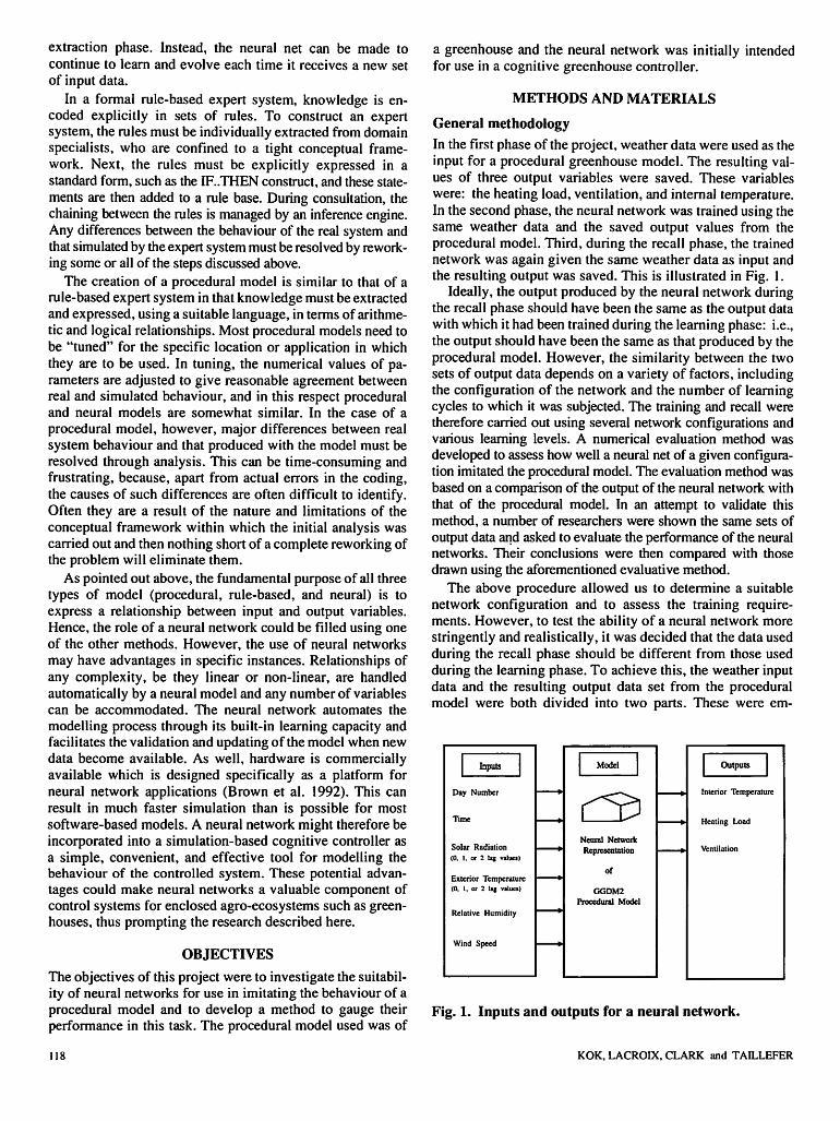
In the first phase of the project, weather data were used as theinput for a procedural greenhouse model. The resulting values of three output variables were saved. These variableswere: the heating load, ventilation, and internal temperature.In the second phase, the neural network was trained using thesame weather data and the saved output values from theprocedural model. Third, during the recall phase, the trainednetwork was again given the same weather data as input andthe resulting output was saved. This is illustrated in Fig. 1.

Ideally, the output produced by the neural network duringthe recall phase should have been the same as the output datawith which it had been trained during the learning phase: i.e.,the output should have been the same as that produced by theprocedural model. However, the similarity between the twosets of output data depends on a variety of factors, includingthe configuration of the network and the number of learningcycles to which it was subjected. The training and recall weretherefore carried out using several network configurations andvarious learning levels. A numerical evaluation method wasdeveloped to assess how well a neural net of a given configuration imitated the procedural model. The evaluation method wasbased on a comparison of the output of the neural network withthat of the procedural model. In an attempt to validate thismethod, a number of researchers were shown the same sets ofoutput data and asked to evaluate the performance of the neuralnetworks. Their conclusions were then compared with thosedrawn using the aforementioned evaluative method.

The above procedure allowed us to determine a suitablenetwork configuration and to assess the training requirements. However, to test the ability of a neural network morestringently and realistically, it was decided that the data usedduring the recall phase should be different from those usedduring the learning phase. To achieve this, the weather inputdata and the resulting output data set from the proceduralmodel were both divided into two parts. These were em-

Inpuls

Day Number

Time

Solar Radiation

(0. I. or 2 Ug values)

Exterior Temperature(0. 1, or 2 l*j values)

Relative Humidity

Wind Speed

Model

C^Neural Network

Representation

GGDM2

Procedural Model

Outputs

Interior Temperature

Heating Load

Ventilation

Fig. 1. Inputs and outputs for a neural network.

KOK, LACROIX, CLARK and TAHXEFER

ployed as follows. Part of the weather data, together with thecorresponding output from the procedural model, was used totrain the network. The remainder of the weather data was then

fed to the trained network during its recall phase and theresulting output was compared to the corresponding outputfrom the procedural model. This approach was repeated several times, the weather data set being partitioned in a differentmanner each time so as to gradually increase the challenge tothe neural network.

Hardware, software, and data sets

The work was carried out on two IBM PS/2 microcomputers,a Model 80161 and a Model 55SX, both of which containedIntel 80386 microprocessors and 80387 math co-processors.DOS 5.00 was used as the operating system on the Model80161, and DOS 4.01 was used on the Model 55SX.

The Gembloux Greenhouse Dynamic Model (GGDM2),as described by Halleux (1989), was modified for use as theprocedural model in the simulation of the greenhouse behaviour. In the research described here, GGDM2 was compiledand linked with Microsoft Fortran 5.0. GGDM2 models a

greenhouse with a double cover and simultaneously takesinto account energy balances for each of the following elements: each of the two covers, the air between the covers, theair in the growth zone, the crop, and four layers of soil.Water balances are also calculated for the two air volumes.

The neural network software used was NeuralWorks Ex

plorer (NeuralWare Inc., Pittsburgh, PA). This is ageneral-purpose package which can be used to create and editnetworks of various types, as well as to train and executethem. The "InstaNet" option of the Explorer software allowsthe creation of common network types. This option was usedin all cases to create standard back-propagation networkshaving various numbers of input, output, and intermediateprocessing elements. Each network had a layer of input elements, two hidden layers of processing elements, and a layerof output elements. All of the layers were fully connected.The delta-rule was used for learning. Elements in the hiddenlayers used sigmoid transfer functions and those in the inputand output layers used linear functions. For definition of theterminology and further information regarding the methodology, the reader is referred to NeuralWare (1990a, 1990b).

The following parameter values were used in the simulation utilizing the procedural model (GGDM2): the maximumheating power was 400 W/m . The heater was switched onwhen the internal temperature fell more than 1 °C below thesetpoint and was switched off again when the temperaturerose more than 1°C above the setpoint. Mechanical ventilation of the simulated greenhouse used two fans: for low flowsa fan with a capacity of 3.5 air changes per hour was used andfor higherflows a two-stage fan (22.5 or 34.0 air changes perhour) was available. The small fan was switched on when thetemperature rose3.5 °C above the setpointand was switchedoff again when it camebackwithin 2 °C of the setpoint. Thetwo stages of the larger fan switched on (off) at 4.5 (3.5) °Cand 6.0 (4.5) °C above the setpoint, respectively. For thesimulation, the temperature setpoint was set at 20 °C fromsunrise until sunset and 16°C for the restof the day.Sunriseand sunset were defined as the times when the external globalradiation rose above and fell below 15 W/m2, respectively.

The meteorological data used were obtained from the Canadian Climate Centre of the Atmospheric EnvironmentService. They were for the Montreal area for 1 March to 29May 1982 and comprised hourly readings of exterior temperature, global radiation, relative humidity, and windvelocity. As previously described, these data were used asinput values for the simulations performed using the procedural model GGDM2 and the neural networks.

The values of three output variables were captured fromthe procedural greenhouse simulation: internal temperature(°C), heatingload (positive heat flux as suppliedby a propaneheater) (W/m ), and ventilation (m «h~ «m" ). All of thevariables were averaged over one-hour periods of simulatedtime and captured once every simulated hour.

The weather data and the resulting output values from theGGDM2 procedural simulation were combined side by sideinto one master data set, such that each line contained acomplete set of input and output values. The first 120 lines ofdata were then discarded to eliminate any startup effects.Seven shorter data sets were subsequently derived from themaster data set for use in training the neural network.GGDM2 is a dynamic model in which the values of thesimulation variables are dependent on their previous values.Some previous values (lag values) were therefore included inthe data sets as inputs for the neural nets. The first data setwas generated simply by removing the first 24 lines of datafrom the master data set; no lag values were included. Sinceit contained no lag values, this first data set will henceforthbe referred to as Data Set 0. The next data set (Data Set 1) wascreated by removing the top 24 lines from the master data set.Lag values were then added to each line of data. They comprised one value for each of solar radiation and externaltemperature; these were the values for the previous one-hourinterval. Each line of Data Set 2 contained weather data, thecorresponding output values from the procedural GGDM2simulation, and lag values for each of solar radiation andexterior temperature for each of the two previous intervals.The subsequent data sets, Data Set 3 through Data Set 6, weresimilarly prepared, each line containing the number of lagvalues for each of the solar radiation and ventilation variables

as is denoted in the data set name.

Evaluation method

The performance of a neural network can be judged by comparing the output generated during the recall phase with theoutput values used for training (i.e., the output values fromthe simulation using the procedural model). This may bedone in any of a number of ways. For example, the values ofa given output variable from the neural network and from theprocedural model might be presented graphically and thecomparison done visually by human judges. The detection ofsimilarities or differences in the pattern would then dependon the processing ability of the human visual cortex. This is,however, a qualitative approach and, moreover, it is practicalonly for a very limited amount of data. Another drawback isthat it cannot be relied upon to be consistent,i.e., to repeatedlyyield the same result for the same data, with either the sameor different judges. To compare the data from a substantialnumber of experiments, it is preferable to rely on a numericalmethod. Such an approach can be used for large amounts of

CANADIAN AGRICULTURAL ENGINEERING Vol. 36, No. 2. April/May/June 1994 119

data, yields quantitative results, and is more consistent (although it may also be less sophisticated and comprehensive).

The objective of this part of the study was to develop aconsistent numerical evaluation method for use in comparingthe recall output of a trained neural network with the outputof the procedural model. The intent was that the methodshould yield a single score for each variable, indicative of theextent of agreement between the two sets of output data.Furthermore, this score should correspond in some directmanner to the visual assessment performed by human judges.Preference favoured a system for which the score would liein a range between 0 and 100.

When visually judging the extent of agreement betweentwo data sets, at least two separate but interacting phenomenaare taken into account by humans. Both of these should betaken into account when devising a numerical judgingscheme. They are the similarity of: (a) the magnitudes of thesignals and (b) their shapes. This is illustrated in Fig. 2. InCase 1, both the shape and magnitude of the two data sets aredifferent. In Case 2, the two signals are similar in shape, butdifferent in magnitude. In Case 3, they are similar in magnitude but different in shape;i.e., one is shifted with respect tothe other.

In the devised evaluation scheme, a score awarded to aparticular neural network was calculated as follows:

a) the output data from the neural network was examinedand the lowest value was extracted (LOW);

b) this value was then subtracted from each of the N valuesin the output data set from the neural network (SETa)to give SETc;

c) LOW was also subtracted from each value in the outputdata set from the procedural simulation (SETr) to giveSETd;

SETc (I) = SETA (I) - LOW 1< I< N (1)

SETD (I) = SETB (I) - LOW 1< I< N (2)

d) the root mean square (RMS) value of SETc was thenfound, for later use in scaling;

RMS = (3)

e) using Eq. 4, both SETc and SETd were filtered toremove high frequency components, resulting in SETeand SETf;

X(I) = X(I - 2) + 2 • X(I - 1) + 3 • X(I)

+ 2»X(I + l) + X(I + 2)

3 < I< N-2 (4)

0 the absolute differences between SETe and SETf werecalculated, yielding SETg;

SETg(I) = ABS [SETf(I) - SETE(I)] (5)

120

6 8 10 12 14

Data Point Number

16

Fig. 2. Three cases of differences between two signals.

g) the root mean square value of the absolute differences(RMSDIFF) was found using:

RMSDIFF=

N-2

I SETbdY1= 3

A/-4

h) the final score (SCORE) was calculated using:

SCORE =100 1-RMSDIFF

RMS

(6)

(7)

Except for extreme circumstances, the method describedalways yields a score between 0 and 100. The magnitude ofthe score is directly related to the overall difference betweenthe two data sets; a value of 100 indicates a perfect matchbetween the two signals, and a value of 0 means there is littleor no likeness between them. The combination of formulae

used in the method was the result of a large number of trialsand was found to yield results which agreed well with thevisual judgment of the authors.

Configuration and training requirements (ExperimentSetl)

A total of 42 primary experiments were performed in this set.(As described below in the Results and Discussion section, anumber of secondary experiments were done as well, to moreclosely examine a problem area.) The objective was to measure how quickly the neural network would learn and whateffect the inclusion of lag values might have. For the primaryexperiments, seven levels of lag were tried, corresponding toData Set 0 through Data Set 6. Six levels of learning weretried: 5,000, 10,000, 50,000, 100,000, 150,000, and 200,000learning cycles.

Each experiment was conducted in the following manner:first, the Instanet option of the NeuralWorks Explorer software package was used to create a neural network with thedesired number of elements in the input, output, and processing layers. The number of elements in the input layer (N) wasequal to the number of inputs in each line of the Data Setused;i.e., 6, 8, 10, 12, 14, 16, or 18 elements, depending onthe number of lag values included. The number of elements

KOK. LACROIX. CLARK and TAILLEFER

CombineData

Trainingof

Neural Network

Recallby

Neural Network

JL^/^Output Data\' from \\Neural Network/

Evaluation

GGDM2Procedural

Model

GGDM2Output Data

Fig. 3. Data treatment and information flow forExperiment Set 1.

in each of the hidden layers was one more than twice thenumber of input elements (2N+1). The output layer alwayshad three elements, corresponding to the three output variables. Next, the network was initialized and then trained forthe requisite number of learning cycles. During training thenetwork was instructed to read randomly from the appropriate Data Set, using the same lines as often as necessary. Forrecall, the trainednetworkwas fed the same input data again,but this time sequentially. During this recall operation itignored the output columns in the DataSet and instead generated its own output. This new output was captured andsubsequently comparedto the originaloutput from the procedural model. The method is illustrated in Fig. 3.

Visual judgment (Experiment Set 2)

The objective of the second set of experiments was to compare the scores assigned using the aforementioned numericalevaluation method withthoseassignedby humans usingtheirvisual judgment. These experiments were based on the datagenerated in Experiment Set 1.

A computer program was written to do the following: (a)randomly choose one of the primary experiments from Experiment Set 1; (b) randomly choose one of the three outputvariables; (c) randomly choose a starting location in theoutput files; (d) beginning at the chosen starting location inthe output files, isolate two corresponding data segments:one taken from the output file produced by the chosen neural

network during its recall phase and the other taken from theoriginal output file of the procedural model. The two datasegments were then displayed simultaneously on a computerscreen. (Each data segment comprised 190 data points, thelongest segment that could be displayed clearly on the computer screen.). Then (e) the human subject was prompted toenter a score value and (f) the numerical evaluation methodwas used to calculate a score for the same data segments.

The human subjects were recruited from among the staffand students of the Agricultural Engineering Department.All of the subjects were volunteers and all were familiar withexperimental data, graphical displays, etc. It was explained toeach subject that the objective of the experiment was tocompare visual judgment with a numerical procedure, but themethod used in the numerical procedure was not explained.The subjects were simply asked to assign a score between 0and 100 for each pair of data segments that they were shown.Twenty subjects participated and each judged 30 pairs of datasegments. Note that although visual judgment is qualitative,the subjects were asked to express the scores quantitativelyso that they might be compared directly with the results fromthe numerical evaluation method.

Different data for learning and recall (Experiment Set 3)

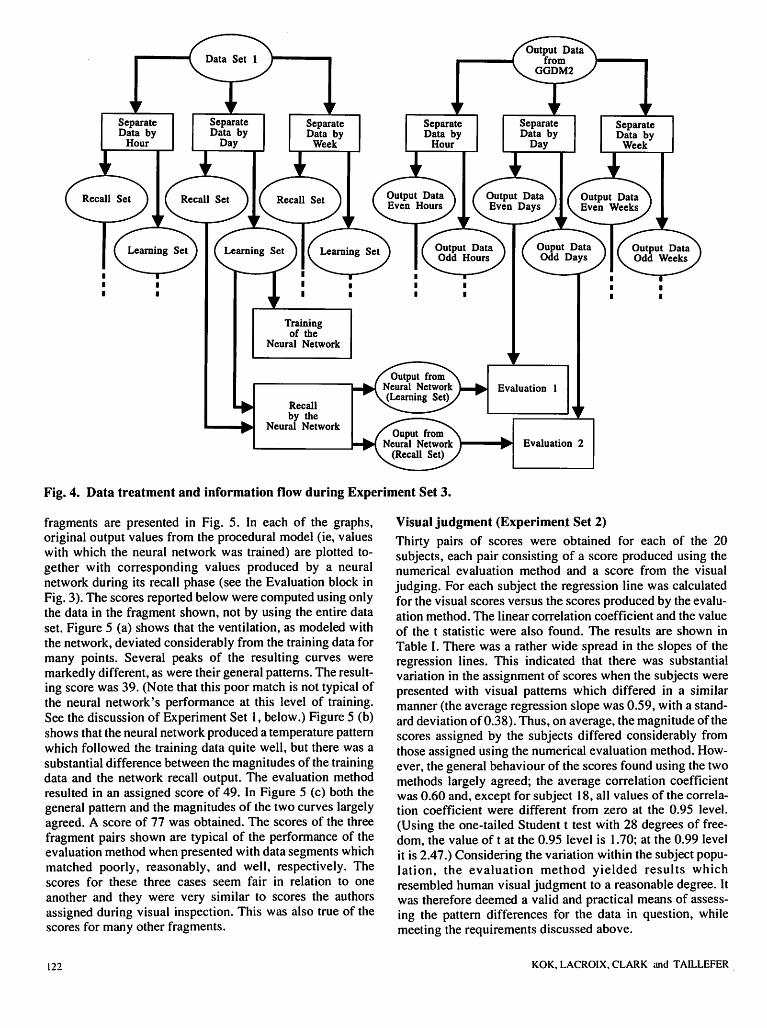
The objective of Experiment Set 3 was to measure how wella network would perform when the input data differed fromthose used in its training. Data Set 1 was chosen for use onthe basis of results from Experiment Set 1. Data Set 1 wasdivided into two parts, resulting in two new data sets, hereafter referred to as the Learning Set and the Recall Set. The newdata sets contained sequences of alternating data segmentscopied from Data Set 1. This process was repeated threetimes, extracting hourly, daily, or weekly blocks of data fromData Set 1. The original output data from the proceduralmodel were similarly divided so that three more data setswere created, respectively containing data for odd and evenhours, for odd and even days, and for odd and even weeks.

The neural network used had the same configuration asthat used with Data Set 1 in Experiment Set 1: i.e., 8 inputelements (six input variables and one lag value for each oftwo variables), 17elements in each of the two hidden layers,and 3 output elements. The network was subjected to 100,000learning cycles using data read randomly from a LearningSet. To get a complete picture of the network's performance,it was subsequentlyinstructedto pass through its recall phasetwice. During the first pass, its input consisted of trainingdata from the Learning Set and during the second pass itsinput consisted of values from the corresponding Recall Set.The two resulting output data sets were then compared withthe output from the procedural model. This was done usingthe numerical evaluation method previously described. Thisexperiment was performed three times, using the newly derived hourly, daily, and weekly Learning and Recall Sets.The procedurefor ExperimentSet 3 is illustrated in Fig. 4.

RESULTS

The evaluation method

To illustrate the results obtained by using the numericalevaluation method in Experiment Set 1, three output data

CANADIAN AGRICULTURAL ENGINEERING Vol. 36. No. 2. April/May/June 1994 121

SeparateData by

Hour

SeparateData by

Day

SeparateData by

Week

( Recall Set J

Trainingof the

Neural Network

Recallby the

Neural Network

SeparateData by

Hour

Output fromNeural Network(Learning Set)

Ouput fromNeural Network

(Recall Set)

SeparateData by

Day

Evaluation 1

Evaluation 2

SeparateData by

Week

Fig. 4. Data treatment and information flow during Experiment Set 3.

fragments are presented in Fig. 5. In each of the graphs,original output values from the procedural model (ie, valueswith which the neural network was trained) are plotted together with corresponding values produced by a neuralnetwork during its recall phase (see the Evaluation block inFig. 3). The scores reported below were computed using onlythe data in the fragment shown, not by using the entire dataset. Figure 5 (a) shows that the ventilation, as modeled withthe network, deviated considerably from the training data formany points. Several peaks of the resulting curves weremarkedly different, as were their general patterns. The resulting score was 39. (Note that this poor match is not typical ofthe neural network's performance at this level of training.See the discussion of Experiment Set 1, below.) Figure 5 (b)shows that the neural network produced a temperature patternwhich followed the training data quite well, but there was asubstantial difference between the magnitudes of the trainingdata and the network recall output. The evaluation methodresulted in an assigned score of 49. In Figure 5 (c) both thegeneral pattern and the magnitudes of the two curves largelyagreed. A score of 77 was obtained. The scores of the threefragment pairs shown are typical of the performance of theevaluation method when presented with data segments whichmatched poorly, reasonably, and well, respectively. Thescores for these three cases seem fair in relation to one

another and they were very similar to scores the authorsassigned during visual inspection. This was also true of thescores for many other fragments.

122

Visual judgment (Experiment Set 2)

Thirty pairs of scores were obtained for each of the 20subjects, each pair consisting of a score produced using thenumerical evaluation method and a score from the visual

judging. For each subject the regression line was calculatedfor the visual scores versus the scores produced by the evaluation method. The linear correlation coefficient and the value

of the t statistic were also found. The results are shown in

Table I. There was a rather wide spread in the slopes of theregression lines. This indicated that there was substantialvariation in the assignment of scores when the subjects werepresented with visual patterns which differed in a similarmanner (the average regression slope was 0.59, with a standard deviation of0.38). Thus, on average, the magnitude of thescores assigned by the subjects differed considerably fromthose assigned using the numerical evaluation method. However, the general behaviour of the scores found using the twomethods largely agreed; the average correlation coefficientwas 0.60 and, except for subject 18, all values of the correlation coefficient were different from zero at the 0.95 level.

(Using the one-tailed Student t test with 28 degrees of freedom, the value of t at the 0.95 level is 1.70; at the 0.99 levelit is 2.47.) Considering the variation within the subject popu-lation, the evaluation method yielded results whichresembled human visual judgment to a reasonable degree. Itwas therefore deemed a valid and practical means of assessing the pattern differences for the data in question, whilemeeting the requirements discussed above.

KOK. LACROIX, CLARK and TAILLEFER

1,500 1,550 1,600 1,650

Data Point Number

1,700

Fig. 5(a). Results for ventilation data, using three lagvalues and 150,000 learning cycles.

2001—

1,050 1,100

Data Point Number

1,150 1,200

Fig. 5 (c). Results for heat flux data, using no lag valuesand 5000 learning cycles.

Experiment Set 1

In Fig.6 thescoresfor the42 primary experiments of Experiment Set 1 are plotted for ventilation. Generally, the scoreincreased as the number of training cycles increased from5,000 to 100,000and remained fairly stable thereafter. Also,the score generally improved when the number of lag valueswas increased from zero to one. The addition of more lagvalues did not affect the score in a regular manner. Experiment Set 3 was therefore run with one lag value for each ofsolarradiation andexteriortemperature and 100,000 learningcycles were used.

On several occasions during Experiment Set 1, there wasa very substantial drop in the score as the neural networkunderwent more training cycles and then again a recoverywhen the training was continued. The most dramatic instanceof this was observed in the series of experiments which usedthree lag values for each of the two lagged variables and100,000, 150,000, and 200,000 learning cycle. The evalu-

100 150

Data Point Number

200

Fig. 5 (b). Results for temperature data, using no lagvalues and 5000 learning cycles.

Table I: Correlation coefficients and Student t values for

Experiment Set 2

Subject Regression Correlation t statistic

number slope coefficient value

1 1.06 0.76 6.16

2 0.73 0.78 6.55

3 1.92 0.62 4.19

4 0.64 0.55 3.47

5 0.38 0.42 2.48

6 0.48 0.41 2.37

7 0.61 0.73 5.62

8 0.55 0.52 3.22

9 0.37 0.65 4.55

10 0.57 0.72 5.53

11 0.15 0.32 1.79

12 0.49 0.77 6.42

13 0.62 0.74 5.88

14 0.16 0.40 2.33

15 0.75" 0.78 6.55

16 0.58 0.84 8.36

17 0.46 0.43 2.51

18 0.25 0.25 1.36

19 0.33 0.44 2.61

20 0.72 0.79 6.92

\verage value 0.59 0.60

ation of the output values for ventilation resulted in scores of87, 38, and 92 respectively. To investigate this phenomenonfurther, a number of secondary experiments were run inexactly the same fashion as the primary experiments, all withthree lag values in the training data. The scores obtained forthese experiments are presented in Fig. 7. For ventilation, thescore was stable at about 89 until 149,979 learning cycles had

CANADIAN AGRICULTURAL ENGINEERING Vol. 36, No. 2, April/May/June 1994 123

100

20

— Data Set 0 + Data Set I * Data Set 2 * Data Set 3

*• Data Set 4 -♦- Data Set 5 * Data Set 6

20 40 60 80 100 120 140 160 180 200

Thousands of Training Cycles

Fig. 6. Numerical scores obtained for the ventilationoutput variable during the primaryexperiments of Experiment Set 1.

been completed, whereupon it dropped to 34 during the next7 cycles, stayed close to this value for 14 cycles, and recovered to 88 over the next 18 cycles. (Note that the datafragment used previously to illustrate the performance of theevaluation method was from this experiment.)

The abrupt drop and correspondingly swift recovery ofthe score are difficult to explain; they illustrate the capri-ciousness which neural networks sometimes display. Toensure that the phenomenon was real and not due to aquirk of the evaluation method, the results from the secondary experiments were also inspected visually. Thebehaviour of the network was found to change radicallyas the training progressed from 149,979 to 150,005 learning cycles, very much in conformance with the scorevalues calculated using the numerical method. This againvalidated the performance of the evaluation method. Thearea of instability in this particular experiment was foundmore or less by accident. Judging from the rest of thedata from the 42 primary experiments, network behaviour was generally quite stable after 100,000 learningcycles. However, it is not clear how many other smallareas of instability there may have been. The occurrenceof such radical behaviour change emphasizes the need forassessment of a network's performance after it has beentrained. The evaluation method could be a useful tool for

this purpose as well.

Different data for learning and recall (Experiment Set 3)

The scores obtained during the three experiments of Experiment Set 3 are reported in Table II. In all three instances,for all three variables, when the data set used for recallwas the same as that used for learning, the score wasaround 90, varying from 88 to 94. The score did not dropmarkedly when different data sets were used for learningand recall, except for the ventilation variable. That scoredropped from 90 to 79 to 74 as Data Set 1 was dividedinto Learning Sets and Recall Sets on an hourly, daily,

124

100

80

60

40

20

* Ventilation ■♦■Temperature *Heat

0149.940 149,960 149,980 150,000 150,020 150,040 150,060

Number of Learning Cycles

Fig. 7. Numerical scores obtained for the three outputvariables during the secondaryexperiments of Experiment Set 1.

and weekly basis, respectively. Presumably, the more difference there is between the input values in the Recall Set andthose in the Learning Set, the less applicable the learning willbe to the recall situation.

Of the three variables, the ventilation displayed the greatest variability. The effect of the difference between theLearning and Recall Sets on the score emerged clearly in thiscase. Corresponding fragments of heat flux output data fromthe procedural and neural models are presented in Fig. 8.These data are from the case when Data Set 1 was divided

into Learning and Recall Sets on a weekly basis and the datasets used for learning and recall were different. When thewhole data sets were compared, a score of 86 was obtained(Table II).

DISCUSSION AND CONCLUSIONS

A backpropagation neural network was used to imitate theperformance of a procedural greenhouse model. The coincidence between the output data from the proceduralmodel and the neural network was very good for all threeoutput variables under the following conditions: usingtypical Montreal weather data; under typical greenhouseoperating conditions; including one set of lag values in thetraining data for each of the exterior temperature and solarradiation variables; using 100,000 learning cycles. Thisclose agreement was reflected in the scores calculatedusing a numerical evaluation method. The scores for thethree output variables were, respectively, 91, 94, and 87when the same input set was used for learning as for recall.The scores were 85, 86, and 74 when the data sets used forlearning and recall were different, having being createdfrom the procedural output data by dividing the data intoalternating weekly blocks. The coincidence of the outputdata was also reflected in the visual resemblance of the two

data sets when they were displayed graphically. It therefore seems that neural networks show promise in replacingprocedural models for the purpose of reasoning about the

KOK, LACROIX, CLARK and TAILLEFER

Table II: Scores obtained during Experiment Set 3 indicating agreement between data sets

Score values (0 to 100) for:

Heat

92

91

91

90

88

86

xperiment Method of Data set used

number division of data for recall

Tem

1 hourly basis Learning Set 1 94

Recall Set 1 93

2 daily basis Learning Set 2 93

Recall Set 2 91

3 weekly basis Learning Set 3 93

Recall Set 3 85

250

50 \-

Procedural Output — Neural Network Output

250 300

Data Point Number

350

Fig. 8. Comparison of heat flux output data fromprocedural and neural models.

reactions that might be expected from a greenhouse in response to possible weather scenarios. The simplicity of thecalculations and the execution speed of the recall proceduremake the neural net a very attractive candidate for suchreasoning activities. We will be testing this approach furtherwith models of more complex systems (eg, entire ecosystems).

Although the evaluation method was arrived at empiricallyusing a trial and error approach and was rather arbitrary inform, it yielded results which were quite similar to thoseobtained using visual judgment. It provided for a simple,efficient, and consistent method of assessment. By using thelearning data set as input for the neural network in recallmode, the numerical evaluation method can be used to compare the output from the neural network with that from theprocedural model. The learning of the neural network canthus be monitored while it progresses. It can also be testedafterwards by recalling with a different data set and comparing the output with the corresponding procedural output. Bysplitting an input data set in various ways, the evaluationmethod can be used to assess the sensitivity of a networkconfiguration to divergence in the learning and recall inputsets.

Vent.

92

90

94

79

89

74

Neural nets have some advantages over procedural models, but they also have several shortcomings which must beaddressed. Firstly, although they can respond to a widespectrum of inputs, the user must ensure that their training has been sufficiently broad to allow a realisticresponse. For example, in Experiment Set 3, it is evidentthat as the learning and recall input sets deviate, theresponse during recall becomes less meaningful. Thismay not be immediately obvious when a neural net hasreceived a narrow training and is forced to respond beyond its knowledge. Secondly, one must assure that thelearning has been effective;i.e., before being used in areasoning task, the performance of a network must be tested.With a neural network, a learning situation occurs which isnot unlike a student/teacher interaction. The learning systemis complex and non-linear and a neural network is not entirelypredictable. One is never sure of what has been absorbed andmust be on guard against learning failures at all times. Thisis made evident by Fig. 7. To deal with some of these issues,we are coupling neural networks to rule-based expert systems.

ACKNOWLEDGEMENTS

The authors gratefully acknowledge the financial assistanceprovided by the National Sciences and Engineering ResearchCouncil and the Conseil des Recherches en Peches et en

Agro-Alimentaire du Quebec in support of this research.

REFERENCES

Brown, T.X., M.D. Tran, T. Duong and A.P. Thakoor. 1992.Cascaded VLSI neural network chips: hardware learningfor pattern recognition and classification. Simulation58(5):340-346.

Halleux, D. de. 1989. Modele dynamique des echangesenergetiques des serres: Etude theorique etexperimentale. These de doctorat, Universite deGembloux, Belgique.

Johnson S.W. and J.P. Wetzel. 1990. Science and

engineering for space: Technologies from Space 88.Journal ofAerospace Engineering 3(2):91 -107.

CANADIAN AGRICULTURAL ENGINEERING Vol. 36. No. 2. April/May/June 1994 125

NeuralWare. 1990a. Neural Computing. NeuralWorks Salisbury F.B. 1991. Lunar farming: Achieving maximumProfessional II, NeuralWorks Explorer. NeuralWare, yield for the exploration of space. Horticultural ScienceInc., Pittsburgh, PA. 26(7):827-833.

NeuralWare. 1990b. User's Guide. NeuralWorks Wilkins M.B. 1988. Columbus and the life sciences. SpaceProfessional II, NeuralWorks Explorer. NeuralWare, Technology 1(2):105-109.Inc., Pittsburgh, PA.

126 KOK, LACROIX, CLARK and TAILLEFER