Lecture 12-1

Interest Rates

1. RBA Objectives and Instruments

The Reserve Bank of Australia has severalobjectives, including “the stability of the currency,the maintenance of full employment”. These twoobjectives mean that price stability is animportant goal, but that in pursuing this, the RBAmust take into account the effects that its actionshave on output and employment.

There are two possible channels through whichmonetary policy might influence the price leveland economic activity:

• By affecting the financial flows betweenborrowers and lenders. Some people in theeconomy spend more than their income — theyare net borrowers; others are net lenders.Monetary policy can influence the cost ofborrowing (i.e. the interest rate) or — in theold, regulated financial system — it coulddirectly restrict these flows, through creditceilings on bank lending. If the price orquantity of financial flows alters, then peoplealter their behaviour. Investors may find thata project which was unprofitable at one rate ofinterest is now profitable at a lower rate ofinterest, and so they will proceed with theinvestment

• By altering the money supply. Thistransmission mechanism relies on the notionthat people may find that they have too much

Lecture 12-2

money in their pockets and will go out andspend it. If monetary authorities allow moremoney to be created in the economy, this willtend to boost spending.

The RBA can influence both these transmissionmechanisms: they can influence financial flowsbetween borrowers and lenders by influencinginterest rates; at the same time, they can influencethe rate of growth of the various monetaryaggregates, with the highest degree of control overthe the narrowest aggregates (such as M1), andless control over broader aggregates (such as M31).At various times, both of the transmissionmechanisms have been the main focus of monetarypolicy.

_________1. M1 is cash plus at-call deposits at the trading banks;

M2 is M1 plus trading bank term deposits; M3 is M2plus savings bank deposits; broad money (BM) is M3plus the net deposit liabilities of the non-bankfinancial institutions.

Lecture 12-3

2. Two Theories of Monetary Policy

2.1 OMOs to deposits to interest rates

Money creation looks like this: the RBA engages inopen market operations OMOs (for example, it sellsbonds, thus reducing the volume of base money)which remove base money from the system. Thisleaves the banks short of required reserves, sothey are forced to contract their balance sheets.This bids up interest rates, and bank deposits (themajor component of M3) dwindle.

This sequence looks like:

OMO → bank reserves → deposits (M3)/credit supply/interest rates

This is one theory of what happens.

2.2 OMOs to interest rates to deposits

Another is that OMOs directly influence theinterest rate, by affecting the interest rate at thevery short end of the yield curve: the “cash” rate.This is the basic block of the yield curve (a plot ofinterest rates against period of the asset, so thatovernight cash rates is one extreme and ten-yearbond rates is another). If cash rates areinfluenced, then other short-end rates are alsoaffected. If OMOs bid down interest rates, thismakes it easier for households and firms toborrow, and so (cet. par.) some previouslypostponed expenditure is now undertaken. This isreflected in the banks’ balance sheets by a growthin the demand for bank credit. The banks thenneed more deposits to fund their lending, and thisis reflected in deposits (i.e. in the monetary

Lecture 12-4

aggregates).

The sequence here is:

OMO → Interest rates → Demand for credit →Deposits (M3)

Which is the exact transmission mechanism is notso very important, since the end result is thesame. What is important is the interest elasticityof the demand for credit, which is the critical linkbetween the RBA’s actions and economic activity.Also important is that in both cases the RBA hasthe ability to influence interest rates, the quantityof lending, and the various components of thefinancial system’s balance sheet which go to makeup the different monetary aggregates.

More anon (from the RBA itself, no less).

Lecture 12-5

Software to Accompany Gordon (6th ed.)

Lecture 12-6

3. How to Access the Software

Borrow the disk from the Closed Reserve section ofthe Library: it’s under Macroeconomics, and isnamed “Gordon”. It’s a DOS disk, for use in theLab. There is also an eight-page leaflet ofcomputer exercises, some of which we’ll consider inclass. Type gordon when in the top directory.

Lecture 12-7

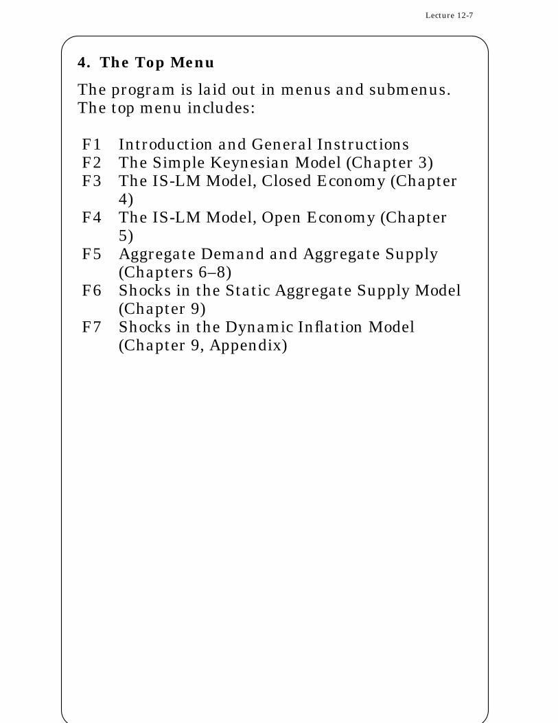
4. The Top Menu

The program is laid out in menus and submenus.The top menu includes:

F1 Introduction and General InstructionsF2 The Simple Keynesian Model (Chapter 3)F3 The IS-LM Model, Closed Economy (Chapter

4)F4 The IS-LM Model, Open Economy (Chapter

5)F5 Aggregate Demand and Aggregate Supply

(Chapters 6–8)F6 Shocks in the Static Aggregate Supply Model

(Chapter 9)F7 Shocks in the Dynamic Inflation Model

(Chapter 9, Appendix)

Lecture 12-8

5. The First Sub-Menu — Simple Keynesian

F1 IntroductionF2 Set Initial Values for Coefficients and

Parameters of the ModelF3 Initial Equilibrium: Numerical SolutionF4 Initial Equilibrium: Graphical Solution —

Figure 3-3 (How equilibrium is determined)F5 Change Coefficients and Parameters of the

ModelF6 New Equilibrium: Numerical SolutionF7 New Equilibrium: Graphical Solution —

Figures 3-3 (How equilibrium is determined),3-4 (The change in equilibrium income causedby an increase in autonomous plannedspending Ap)

F8 Mathematical Structure of Initial and NewModel

Lecture 12-9

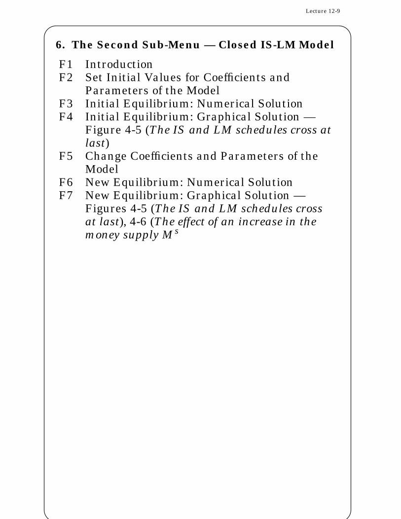
6. The Second Sub-Menu — Closed IS-LM Model

F1 IntroductionF2 Set Initial Values for Coefficients and

Parameters of the ModelF3 Initial Equilibrium: Numerical SolutionF4 Initial Equilibrium: Graphical Solution —

Figure 4-5 (The IS and LM schedules cross atlast)

F5 Change Coefficients and Parameters of theModel

F6 New Equilibrium: Numerical SolutionF7 New Equilibrium: Graphical Solution —

Figures 4-5 (The IS and LM schedules crossat last), 4-6 (The effect of an increase in themoney supply Ms L P with a normal LM curveand a vertical LM curve), 4-7, 4-8 (The effecton real income Y and the interest rate r of anincrease in government spending G)

Lecture 12-10

7. The Third Sub-Menu — Open IS-LM Model

F1 IntroductionF2 Set Initial Values for Coefficients and

Parameters of the ModelF3 Initial Equilibrium: Numerical SolutionF4 Initial Equilibrium: Graphical Solution —

Figure 4-5 (The IS and LM schedules cross atlast)

F5 Change Coefficients and Parameters of theModel

F6 New Equilibrium: Numerical SolutionF7 New Equilibrium: Graphical Solution —

Figures 5-9,10,11 (Effects of increases in themoney supply or government spending underfixed/flexible exchange rates.)

Lecture 12-11

8. The Aggregate Demand and Supply Sub-Menu

The fifth item in the main menu (AggregateDemand and Supply) has a different sub-menu,which in turn has several sub-sub-menus. Butthen this is where the models are starting to getpowerful and contentious.

F1 IntroductionF2 Review of Aggregate Demand Curve (AD) —

ending with Gordon Fig. 6-1 (Effect on realincome Y of different values of the price indexP).

F3 Review of Short-Run Aggregate SupplyCurve (SAS) → a sub-sub menu:

F1 Derivation of Short-Run AggregateSupply Curve (SAS) — ending withFigure 6-7 (The labour demand curveN d, the production function F, and theaggregate supply curve SAS for thewhole economy)

F2 Increase of Normal Wage and its Effecton Aggregate Supply — ending withFigure 6-8 (The short-run aggregatesupply curve SAS for two differentvalues of the wage rate W 0 and W 1)

F3 Decrease of Normal Wage and its Effecton Aggregate Supply — ending withFigure 6-8 (The short-run aggregatesupply curve SAS for two differentvalues of the wage rate W 0 and W 1)

F4 Technical Advance and its Effect onAggregate Supply

Lecture 12-12

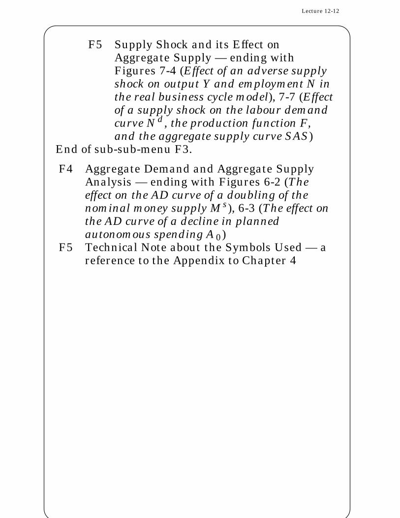
F5 Supply Shock and its Effect onAggregate Supply — ending withFigures 7-4 (Effect of an adverse supplyshock on output Y and employment N inthe real business cycle model), 7-7 (Effectof a supply shock on the labour demandcurve N d, the production function F,and the aggregate supply curve SAS)

End of sub-sub-menu F3.

F4 Aggregate Demand and Aggregate SupplyAnalysis — ending with Figures 6-2 (Theeffect on the AD curve of a doubling of thenominal money supply Ms), 6-3 (The effect onthe AD curve of a decline in plannedautonomous spending A 0)

F5 Technical Note about the Symbols Used — areference to the Appendix to Chapter 4

Lecture 12-13

9. The Next Sub-Menu — Shocks in the StaticAggregate Supply Model

The sixth item in the top menu (Supply andDemand Shocks in the AggregateDemand–Aggregate Supply Model) includes asub-menu:

F1 IntroductionF2 Supply and Demand Shocks in the Static

AD–SAS Model — Figures 7-7 (Effect of asupply shock on the labour demand curve Nd,the production function F, and the aggregatesupply curve SAS), 7-8 (Effect on real GDP Yand the price level P of a higher oil price).

F3 Technical Notes — adaptive expectations (pp.249–251)

Lecture 12-14

10. The Last Sub-Menu — Shocks in theDynamic Inflation Model

The seventh and final item on the top menu(Shocks in the Dynamic Inflation Model) includesa short sub-menu:

F1 Introduction — Appendix of Chapter 9:Tables on pp. 279 and 282, Figures 9-11 (Theeffect on the inflation rate p and output ratioY L Y N of an adverse supply shock that shiftsthe SP curve upward by 3 percent), 9-3 (Theadjustment path of inflation p and real GDPY to an acceleration of nominal GDP growthfrom zero to 6 percent when expectations failto adjust), 9-4 (Effect on inflation p and realGDP Y of an acceleration of demand growthfrom zero to 6 percent), 9-7 (Adjustment pathof inflation p and real GDP Y to a policy thatcuts nominal GDP growth x from 10 percentin 1980 to 4 percent in 1981 and thereafter),9-6 (Initial effect on inflation p and real GDPY of a slowdown in nominal GDP growthfrom 10 percent to 4 percent), 9-8 (The effecton real GDP Y and the inflation rate p ofthree alternative growth paths of nominalGDP).

F2 Initialise the ModelF3 Generate Shocks to the ModelF4 Path of Inflation and Real GDPF5 Inflation and Real GDP over TimeF6 Technical Note

Lecture 12-15

11. ComputerExercises

11.1 The Simple Keynesian Model

1. The marginal propensity to consume (c) is setat 0.75. Leave this as the initial value.

a. Change c to 0.80. What happens to realincome (Y)?

b. Change c to 0.70. What happens to Y?

c. Changing c means changing theconsumption patterns of the populace.Did Y increase or decrease significantlywhen you changed c? How likely do youthink it will be that c will change in theshort run? In the long run? Are thereany factors that might lead c to change?Are there any policies the governmentmight pursue to encourage a change inc in the right direction?

2. Autonomous consumption (a) has an initialvalue of 250. Compare Y with this value andwith a new value of 300. What happens to Y?How significant a change is this? Do youexpect there will be a change in a in theshort run? In the long run? Try to imaginewhat a might have been like for a family in1915, in 1970, and today. Would you expectthe values to be similar? How does youranswer affect the likelihood that a mightchange in the short run?

3. Now look at autonomous investment (Ip),with an initial value of 500.

Lecture 12-16

a. Change this to 550. What happens toY?

b. Change this to 450. What happens toY?

c. For a 10% change in investment (Ip),how much has Y changed? How mightgovernment encourage Ip? Is this apolicy you might expect mostgovernments to follow? Why or whynot?

4. Turn now to government spending (G), withan initial value of 250.

a. Change G to 300. What happens to Y?

b. Change G to 200. What happens to Y?

c. For a 20% change in G, how much hasY changed? Compare with Ip : whichseems to affect Y most? Now considerhow easily government can change G orinfluence Ip : which one wouldgovernment tend to focus on to increaseY?

11.2 Chapter 4 — The IS-LM Model (ClosedEconomy)

1. In the equation C = a + 0.75 YD , leave 0.75 asthe initial value of the marginal propensityto consume (c).

a. Change c to 0.80. What happens to Y?What happens to r? Do Y and r movetogether?

Lecture 12-17

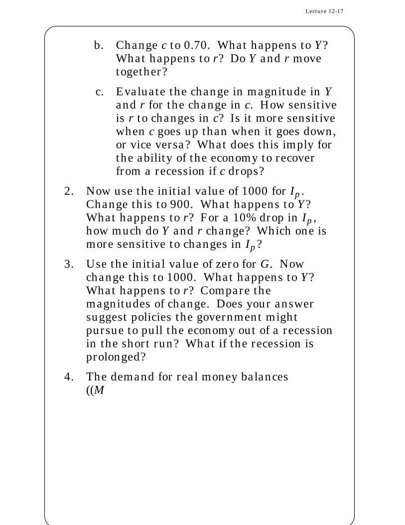
b. Change c to 0.70. What happens to Y?What happens to r? Do Y and r movetogether?

c. Evaluate the change in magnitude in Yand r for the change in c. How sensitiveis r to changes in c? Is it more sensitivewhen c goes up than when it goes down,or vice versa? What does this imply forthe ability of the economy to recoverfrom a recession if c drops?

2. Now use the initial value of 1000 for Ip .Change this to 900. What happens to Y?What happens to r? For a 10% drop in Ip ,how much do Y and r change? Which one ismore sensitive to changes in Ip?

3. Use the initial value of zero for G. Nowchange this to 1000. What happens to Y?What happens to r? Compare themagnitudes of change. Does your answersuggest policies the government mightpursue to pull the economy out of a recessionin the short run? What if the recession isprolonged?

4. The demand for real money balances((M L P)d) is given as 0.5 Y − 100 r. Let’schange the response of money demand to a$1 change in income (Y) at a fixed interestrate (Gordon’s h) and watch what happens tomoney demand.

a. Change 0.5 Y to 0.6 Y. What happens tothe LM curve? What happens to r?

Lecture 12-18

b. Change 0.5 Y to 0.4 Y. What happens tothe LM curve? What happens to r?

c. How sensitive is r to changes in Y?What does this suggest will happen to rin a recession if Y falls considerably?How quickly would you expect r toadjust?

5. The real money supply (Ms L P) is given as1000. Compare the initial value to thefollowing changes:

a. Change 1000 to 1500. What happens toY? What happens to r?

b. Change 1000 to 500. What happens toY? What happens to r?

c. How sensitive is Y and r to changes inthe supply of money? Based on youranswers to this, is the governmentlikely to use changes in the moneysupply to stimulate the economy? Topull an economy out of a recession?Now compare the effects on theeconomy from changes in G andchanges in the money supply. Whichone will the government favour tostimulate the economy? To pull aneconomy out of a recession?

11.3 Chapter 5 — The IS-LM Model (OpenEconomy)

In the Open Economy IS-LM Model, the exchangerate (e) is given by e = 25 r.

Lecture 12-19

a. Change e to 50 r. What happens to Y? Whathappens to r? What happens to the IS curve?

b. Change e to 10 r. What happens to Y? Whathappens to r? What happens to the IS curve?

c. How sensitive were Y and r to changes in e?Were Y and r more sensitive to a positivechange in e or vice versa?

11.4 Chapters 6–8 — The AggregateDemand/Aggregate Supply Model

After the on-disk review of the AD curve, reviewthe SAS curve when:

• the nominal wage W rises and falls,

• there is a technology advance, and

• there is a supply shock (such as the oil-pricerises of the 1970s).

1. Use the 850 initial value of investment Ip :

a. Change 850 to 1050. What happens tothe AD curve? In the short run, whathappens to Y and the price level P?What happens in the long run?

b. Change 850 to 650. What happens tothe AD curve? In the short run, whathappens to Y and P? What happens inthe long run?

c. Considering your answers, how likely isit that the government will try toencourage investment to stimulate theeconomy?

Lecture 12-20

2. Use the 550 initial value for governmentpurchases (G):

a. Change 550 to 850. In the short run,what happens to Y and P? Whathappens in the long run?

b. Change 550 to 400. In the short run,what happens to Y and P? Whathappens in the long run?

c. Considering your answers, what is thelikely short-term effect of an attempt tolower the budget deficit (T −G) byreducing G? Would it be advisable topursue such a policy?

3. The initial value for taxes (T) is 400:

a. Change 400 to 750. In the short run,what happens to Y and P? Whathappens in the long run?

b. Change 400 to 250. In the short run,what happens to Y and P? Whathappens in the long run?

c. Considering your answers, what is thelikely short-term effect of an attempt tolower the budget deficit (T −G) byraising taxes (T)? What is the likelyeffect of an attempt to lower the budgetdeficit (T −G) by both raising taxes (T)and lowering government spending (G)?Would it be advisable to pursue bothpolicies at once?

Lecture 12-21

4. The initial value for the money supply (Ms)is 1000.

a. Change 1000 to 2000. What are theshort-term effects on Y and P? Thelong-term effects?

b. Change 1000 to 500. What are theshort-term effects on Y and P? Thelong-term effects?

c. Considering your answers, how likely isit that the government will usemonetary policy to stimulate theeconomy? How likely is it thatgovernment will contract the moneysupply to deal with inflationarypressures?

5. Of the policies you have just considered,which ones are the easiest to implement?Which ones are the most effective? Is therean inbred bias towards certain policies?