introduction to cf d module
TRANSCRIPT

VERSION 4.2a
Introduction toCFD Module

BeneluxCOMSOL BVRöntgenlaan 372719 DX ZoetermeerThe Netherlands +31 (0) 79 363 4230 +31 (0) 79 361 4212 [email protected] www.comsol.nl
DenmarkCOMSOL A/SDiplomvej 381 2800 Kgs. Lyngby +45 88 70 82 00 +45 88 70 82 88 [email protected] www.comsol.dk
FinlandCOMSOL OYArabiankatu 12 FIN-00560 Helsinki +358 9 2510 400 +358 9 2510 4010 [email protected] www.comsol.fi
FranceCOMSOL FranceWTC, 5 pl. Robert SchumanF-38000 Grenoble +33 (0)4 76 46 49 01 +33 (0)4 76 46 07 42 [email protected] www.comsol.fr
GermanyCOMSOL Multiphysics GmbHBerliner Str. 4D-37073 Göttingen +49-551-99721-0 +49-551-99721-29 [email protected] www.comsol.de
IndiaCOMSOL Multiphysics Pvt. Ltd.Esquire Centre, C-Block, 3rd FloorNo. 9, M. G. RoadBangalore 560001Karnataka +91-80-4092-3859 +91-80-4092-3856 [email protected] www.comsol.co.in
ItalyCOMSOL S.r.l.Via Vittorio Emanuele II, 2225122 Brescia +39-030-3793800 +39-030-3793899 [email protected] www.comsol.it
NorwayCOMSOL ASPostboks 5673 SluppenSøndre gate 7NO-7485 Trondheim +47 73 84 24 00 +47 73 84 24 01 [email protected] www.comsol.no
SwedenCOMSOL ABTegnérgatan 23SE-111 40 Stockholm +46 8 412 95 00 +46 8 412 95 10 [email protected] www.comsol.se
SwitzerlandCOMSOL Multiphysics GmbHTechnoparkstrasse 1CH-8005 Zürich +41 (0)44 445 2140 +41 (0)44 445 2141 [email protected] www.ch.comsol.com
United KingdomCOMSOL Ltd.Broers Building21 J J Thomson AvenueCambridge CB3 0FA +44-(0)-1223 451580 +44-(0)-1223 367361 [email protected] www.uk.comsol.com
United StatesCOMSOL, Inc.1 New England Executive ParkSuite 350Burlington, MA 01803 +1-781-273-3322 +1-781-273-6603
COMSOL, Inc.10850 Wilshire BoulevardSuite 800Los Angeles, CA 90024 +1-310-441-4800 +1-310-441-0868
COMSOL, Inc.744 Cowper StreetPalo Alto, CA 94301 +1-650-324-9935 +1-650-324-9936 [email protected] www.comsol.com
For a complete list of international representatives, visit www.comsol.com/contact
Home Page www.comsol.com
COMSOL User Forums www.comsol.com/
community/forums
Introduction to the CFD Module
1998–2011 COMSOL
Protected by U.S. Patents 7,519,518; 7,596,474; and 7,623,991. Patents pending.
This Documentation and the Programs described herein are furnished under the COMSOL Software License Agreement (www.comsol.com/sla) and may be used or copied only under the terms of the license agreement.
COMSOL, COMSOL Desktop, COMSOL Multiphysics, and LiveLink are registered trademarks or trade-marks of COMSOL AB. Other product or brand names are trademarks or registered trademarks of their respective holders.
Version: October 2011 COMSOL 4.2a
Part No. CM021302
cfd_introduction.book Page 2 Friday, September 23, 2011 12:07 PM

cfd_introduction.book Page 3 Friday, September 23, 2011 12:07 PM
Contents
Introduction . . . . . . . . . . . . . . . . . . . . . . . . . . . . . . . . . . . .1
Tutorial Example—Backstep . . . . . . . . . . . . . . . . . . . . .11
Tutorial Example—Heat Sink . . . . . . . . . . . . . . . . . . . .26

cfd_introduction.book Page 4 Friday, September 23, 2011 12:07 PM

cfd_introduction.book Page 1 Friday, September 23, 2011 12:07 PM
IntroductionThe CFD Module is used by engineers and scientists to understand, predict, and design the flow in closed and open systems. At a given cost, this type of simulations typically yield new and better products and operation of devices and processes compared to pure empirical studies involving fluid flow. As a part of an investigation, simulations give accurate estimates of flow patterns, pressure losses, forces on surfaces subjected to a flow, temperature distribution, and variations in fluid composition in a system.
Flow ribbons and velocity field magnitude from the simulation of an Ahmed body. The simulation yields the flow and pressure fields and calculates the drag coefficient as a benchmark for verification and validation of turbulence models.
The CFD Module’s general capabilities include stationary and time-dependent flows in two-dimensional and three-dimensional spaces. Formulations of different types of flow are predefined in a number of user interfaces, referred to as fluid flow interfaces, which allow you to set up and solve fluid flow problems. The fluid flow interfaces use physical quantities, such as pressure and flow rate, and physical properties, such as viscosity and density, to define a fluid flow problem. There are different fluid flow interfaces that cover a wide range of flows: for example, laminar flow, turbulent flow, single-phase flow, and multiphase flow.
The fluid flow interfaces formulate conservation laws for the conservation of momentum, mass, and energy. These laws are expressed in partial differential equations, which are solved by the CFD Module together with the corresponding
Introduction | 1
cfd_introduction.book Page 2 Friday, September 23, 2011 12:07 PM
initial conditions and boundary conditions. The equations are solved using stabilized finite element formulations for fluid flow, in combination with damped Newton methods and, for time-dependent problems, different time-dependent solver algorithms. The results are presented in the graphics window through predefined plots relevant for CFD, expressions of the physical quantities that you can define freely, and derived tabulated quantities (for example, average pressure at a surface and drag coefficients) obtained from a simulation.
The work flow in the CFD Module is quite straightforward and can be described by the following steps: define the geometry, select the fluid to be modeled, select the type of flow, define boundary and initial conditions, define the finite element mesh, select solver, and visualize the results. All these steps are accessed from the user interface. The meshing and solver steps are usually carried out automatically using default settings, which are tuned for each specific fluid flow interface.
The CFD Module’s Model Library describes the fluid flow interfaces and their different features through tutorial and benchmark examples for the different types of flows. Here you find models of industrial equipment and devices, tutorial models for education, and benchmark models for verification and validation of the fluid flow interfaces.
This introduction is intended to give you a jump-star t in your modeling work. It contains examples of the typical use of the CFD Module, a list of all the fluid flow interfaces including a short description for each interface, and two tutorial examples that introduce the workflow in the CFD Module. The first tutorial solves a laminar flow problem, while the second example introduces conjugate heat transfer—that is, coupled heat transfer in fluids and solids.
Aspects of CFD SimulationsThe CFD Module covers flows ranging from just above the microscale, for example, in medical applications, up to the scales of the flows in ventilation systems and buildings.
One common use of CFD simulations is to understand the flow in a system. The flow pattern may determine the air quality in a ventilated room or it may also determine the forces on a body subjected to the flow. Qualitative interpretation of the flow and pressure fields is usually the first step in innovating or improving a design.
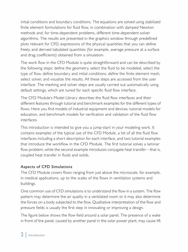
The figure below shows the flow field around a solar panel. The presence of a wake in front of the panel, caused by another panel in the solar power plant, may cause lift
2 | Introduction
cfd_introduction.book Page 3 Friday, September 23, 2011 12:07 PM
forces that would not be present if the panel was analyzed alone in a simulation. 3D graphics such as surface plots, movies, and streamlines, ribbons, arrows, and particle tracing plots are examples of the tools that you can use for qualitative studies.
Turbulent fluid flow around a solar panel solved using the CFD Module.
Another common use of the CFD Module, in almost all scales and in many applications, is the prediction of quantitative estimates of proper ties of the system, such as the average flow at a given pressure differences and the drag and lift coefficients.
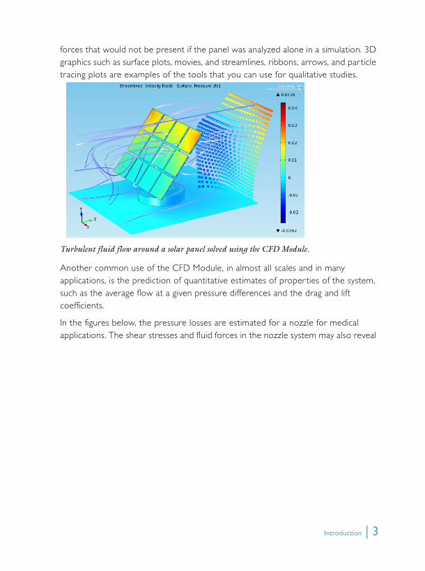
In the figures below, the pressure losses are estimated for a nozzle for medical applications. The shear stresses and fluid forces in the nozzle system may also reveal
Introduction | 3
cfd_introduction.book Page 4 Friday, September 23, 2011 12:07 PM
the risks for causing blood damages in medical equipment, which have to be accounted for when controlling the flow.
Pressure field and flow field in a model of a nozzle relevant for applications in medical design.
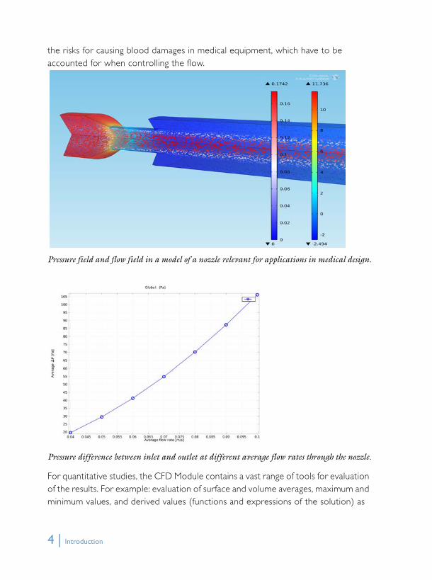
Pressure difference between inlet and outlet at different average flow rates through the nozzle.
For quantitative studies, the CFD Module contains a vast range of tools for evaluation of the results. For example: evaluation of surface and volume averages, maximum and minimum values, and derived values (functions and expressions of the solution) as
4 | Introduction
cfd_introduction.book Page 5 Friday, September 23, 2011 12:07 PM
well as generation of tables and x-y plots. Derived values such as drag and lift coefficients and other values relevant for CFD are predefined in the CFD Module.
Typically, qualitative studies form the basis for understanding, which sparks innovations that result in great improvement of products and processes often in quantum leaps. Quantitative studies form the basis for optimization and control, which can also greatly improve products and processes but then usually in many small steps.
The Fluid Flow InterfacesAs mentioned above, the fluid flow interfaces in the CFD Module are based on the laws for conservation of momentum, mass, and energy in fluids. Different combinations and expressions of the conservation laws result in the different flow models. These laws of physics are translated by the fluid flow interfaces to sets of partial differential equations with corresponding initial and boundary conditions.
A fluid flow interface defines a number of features. Each feature represents an operation that describes a term or condition in the conservation equations. Such a term or condition can be defined in a geometric entity of the model, such as a domain, boundary, edge (3D), or point.
The figure below shows the Model Tree including a “Laminar Flow” interface, to the left, and the “Settings” window for the selected “Fluid Properties 1” feature, to the right. The “Equations” section in the “Settings” window shows the model equations and the terms added by the “Fluid Properties 1” feature to the model equations. The added terms are underlined with a dotted line. The “Fluid Properties 1” feature adds the terms to the model equations to a selected geometrical domain. Furthermore, the “Fluid Properties 1” feature may link to the “Materials” feature to obtain physical properties such as density and dynamic viscosity, in this case the fluid properties of water. The fluid properties, defined by the “Water, liquid” feature, can be functions of the modeled physical quantities, such as pressure and temperature. In the same
Introduction | 5

cfd_introduction.book Page 6 Friday, September 23, 2011 12:07 PM
fashion, the “Wall 1” feature adds the boundary conditions to the walls of the fluid domain.
The CFD Module includes a catalogue with a large number of Fluid Flow interfaces ( ) for different types of flow. In addition, it also includes Chemical Species Transport interfaces ( ) for reacting flows in multicomponent solutions and Heat Transfer interfaces ( ) for heat transfer in solids, fluids, and porous media.
6 | Introduction
cfd_introduction.book Page 7 Friday, September 23, 2011 12:07 PM
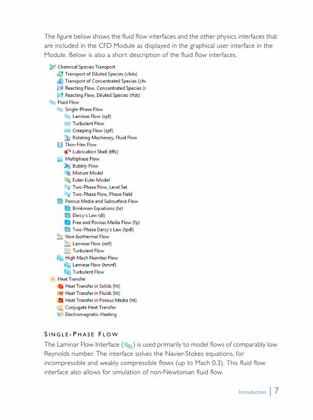
The figure below shows the fluid flow interfaces and the other physics interfaces that are included in the CFD Module as displayed in the graphical user interface in the Module. Below is also a short description of the fluid flow interfaces.
S I N G L E - P H A S E F L O W
The Laminar Flow Interface ( ) is used primarily to model flows of comparably low Reynolds number. The interface solves the Navier-Stokes equations, for incompressible and weakly compressible flows (up to Mach 0.3). This fluid flow interface also allows for simulation of non-Newtonian fluid flow.
Introduction | 7

cfd_introduction.book Page 8 Friday, September 23, 2011 12:07 PM
The Turbulent Flow Interfaces ( ) model flow of high Reynolds numbers. The interface uses the Reynolds-averaged Navier-Stokes (RANS) equations and solves for the averaged velocity field and averaged pressure. The fluid flow interface also formulates different models for the turbulent viscosity. There are several turbulence models available—a standard k- model, a Low Reynolds number k- model, a k- model, and the Spalar t-Allmaras model. Similar to the Laminar Flow interface, compressibility (Mach < 0.3) is selected by default.
The standard k- model is the most widely used turbulence model since it is often a good compromise between accuracy and computational cost (memory and CPU-time). The Low Reynolds number k- model gives a better accuracy than the standard model, especially close to walls, but this accuracy comes with a higher computational cost. The k- model is an alternative to the standard k- model and it can often give more accurate results. However, the k- model is also less robust than the standard k- model. The Spalar t-Allmaras model is specifically designed for aerodynamic applications, such as wing profiles, but is also widely used for other applications due to its high robustness and decent accuracy.
The Creeping Flow Interface ( ) approximates the Navier-Stokes equations for very low Reynolds numbers. This is often referred to as Stokes flow and is appropriate for use when viscous flow is dominant, such as in very small channels or microfluidics applications.
The Rotating Machinery Interfaces ( ) are used for the modeling of flow where one or more of the boundaries rotate, for example in mixers and propellers. The physics interfaces support compressibility (Mach 0.3), laminar non-Newtonian flow, and turbulent flow using the standard k- model.
T H I N - F I L M F L O W
The Lubrication Shell interface ( ) is available in 2D, 2D axisymmetric, and 3D geometries. This physics interface is a boundary interface, which means that the boundary level is the highest level; it does not have a domain level. Using boundary equations, this physics interface models the thickness, velocity, and pressure in narrow channels. The simulation of the flow of a lubrication oil between two rotating cylinders is an example of a possible use of this physics interfaces.
M U L T I P H A S E F L O W
The Bubbly Flow interface ( ) models two-phase flow where the fluids form a gas-liquid homogeneous mixture, and the content of the gas is less than 10%. The
8 | Introduction

cfd_introduction.book Page 9 Friday, September 23, 2011 12:07 PM
physics interface supports both laminar and turbulent flows using an extended version of the k- turbulence model that can account for bubble induced turbulence. For laminar flows, the physics interface supports non-Newtonian liquids. The Bubbly Flow interface also allows for mass transfer between the two phases.
The Mixture Model interface ( ) is similar to the Bubbly Flow interfaces but assumes that the dispersed phase consists of solid particles or liquid droplets. The continuous phase has to be a liquid. The physics interface supports both laminar and turbulent flows using the k- turbulence model. For laminar flows, the physics interface supports non-Newtonian fluids. The Mixture Model interface also allows for mass transfer between the two phases.
The Euler-Euler Model interface ( ) for two-phase flow is able to handle the same cases as the Bubbly Flow and Mixture Model interfaces but is not limited to low concentrations of the dispersed phase. In addition, the Euler-Euler Model interface can handle large differences in density between the phases, such as the case of solid particles in air. This makes the model suitable for simulations of fluidized beds.
The Two-Phase Flow, Level Set interface ( ) and the Two-Phase Flow, Phase Field interface ( ), are both used primarily to model two fluids separated by a fluid interface. The moving interface is tracked in detail using the level set method and the phase field method respectively. Similar to other fluid-flow interfaces, these physics interfaces support both compressible (Mach 0.3) and incompressible flow. They support laminar flow where one or both fluids can be non-Newtonian. The physics interfaces support turbulent flow using the standard k- turbulence model and also Stokes flow.
P O R O U S M E D I A A N D S U B S U R F A C E F L O W
The Brinkman Equations interface ( ) models flow through a porous medium where the influence of shear stresses are significant. The physics interface supports both the Stokes-Brinkman formulation, suitable for very low flow velocities, and Forchheimer drag, which is used to account for effects at higher velocities. The fluid can be either incompressible or compressible, given that the Mach number is less than 0.3.
The Darcy’s Law interface ( ) models relatively slow flows through porous media in the cases where the effects of shear stresses perpendicular to the flow are small.
Introduction | 9

cfd_introduction.book Page 10 Friday, September 23, 2011 12:07 PM
The Free and Porous Media Flow interface ( ) models porous media that contain open channels connected to the porous media, such as in fixed-bed reactors and catalytic converters.
The Two-Phase Darcy’s Law interface ( ) sets up two Darcy’s law, one for each fluid phase in porous media, and couples the two, for example using capillary expressions. It is tailored for modeling effects such as moisture transport in porous media.
N O N I S O T H E R M A L F L O W
The Non-Isothermal Flow, Laminar Flow Interface ( ) is used primarily to model slow-moving flow in environments where the temperature and flow fields have to be coupled. A typical example is natural convection. The physics interface features predefined functionality to couple heat transfer in fluids and solids.
The Non-Isothermal Flow, Turbulent Flow interfaces ( ) use the Reynolds-Averaged Navier-Stokes (RANS) equations coupled to heat transfer in fluids and in solids. The physics interface supports three RANS turbulence models – the standard k- model, a Low Reynolds number k- model, a k- model, and the Spalar t-Allmaras model.
The Conjugate Heat Transfer interface ( ) is also included in the CFD Module and is actually almost identical to the Non-Isothermal Flow interface, since they only differ in the default settings.
H I G H M A C H N U M B E R F L O W
The High Mach Number, Laminar Flow interface ( ) solves momentum and energy equations for fully compressible laminar flow. The physics interface can typically be used for modeling low-pressure systems, where the flow velocity can be very large but where the flow stays laminar.
The High Mach Number, Turbulent Flow interfaces ( ) solves momentum and energy equations for fully compressible turbulent flow coupled to a RANS turbulence model. There are two version of this physics interfaces: one that couples to the k- turbulence model and one that couples to the Spalar t-Allmaras turbulence model.
10 | Introduction

cfd_introduction.book Page 11 Friday, September 23, 2011 12:07 PM
Tutorial Example—BackstepThis tutorial model solves the incompressible Navier-Stokes equations in a backstep geometry. A characteristic feature of fluid flow in geometries of this kind is the recirculation region that forms where the flow exits the narrow inlet region. The model demonstrates the modeling procedure for laminar flows in the CFD Module.
Model GeometryThe model consists of a pipe connected to a block-shaped duct; see the figure below. Due to symmetry, it is sufficient to model one eighth of the full geometry.
Model geometry.
Domain Equation and Boundary ConditionsThe flow in the system is laminar and therefore the Laminar Flow interface is used.
The inlet flow is fully developed laminar flow, described by the corresponding inlet boundary condition. This boundary condition computes the flow profile for fully develop laminar flow in channels of arbitrary cross section. The boundary condition at the outlet sets a constant relative pressure. Furthermore, the vertical and inclined boundaries along the length of the geometry are symmetry boundaries. All other boundaries are solid walls described by a non-slip boundary condition.
Inlet
Outlet
Symmetry
Wall
Symmetry
Wall
Tutorial Example—Backstep | 11

cfd_introduction.book Page 12 Friday, September 23, 2011 12:07 PM
ResultsThe figure below shows a combined surface and arrow plot of the flow velocity. This plot does not reveal the recirculation region in the duct immediately beyond the inlet pipe’s end. For this purpose, a streamline plot is more useful, as demonstrated in the next figure.
The velocity field in the backstep geometry.
12 | Tutorial Example—Backstep

cfd_introduction.book Page 13 Friday, September 23, 2011 12:07 PM
The recirculation region visualized using a velocity streamline plot.
The following instructions show how to formulate, solve, and reproduce these plots using the CFD Module.
MODEL WIZARD
The first step is to select the space dimension and the Laminar Flow interface for stationary studies.
1 Go to the Model Wizard window.
2 Click Next .
3 In the Add physics tree, select Fluid Flow>Single-Phase Flow>Laminar Flow (spf) .
4 Click Next .
Tutorial Example—Backstep | 13
cfd_introduction.book Page 14 Friday, September 23, 2011 12:07 PM
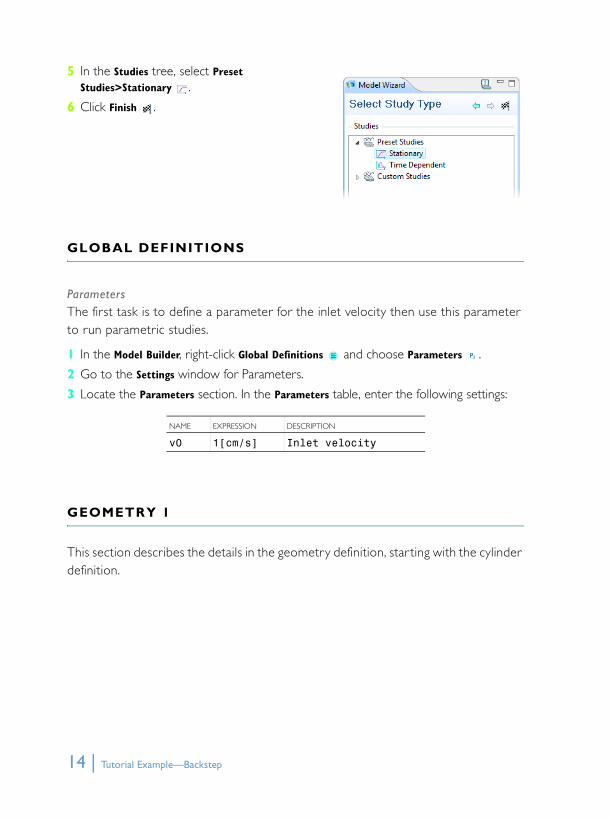
5 In the Studies tree, select Preset Studies>Stationary .
6 Click Finish .
GLOBAL DEFINITIONS
ParametersThe first task is to define a parameter for the inlet velocity then use this parameter to run parametric studies.
1 In the Model Builder, right-click Global Definitions and choose Parameters .
2 Go to the Settings window for Parameters.
3 Locate the Parameters section. In the Parameters table, enter the following settings:
GEOMETRY 1
This section describes the details in the geometry definition, star ting with the cylinder definition.
NAME EXPRESSION DESCRIPTION
v0 1[cm/s] Inlet velocity
14 | Tutorial Example—Backstep
cfd_introduction.book Page 15 Friday, September 23, 2011 12:07 PM
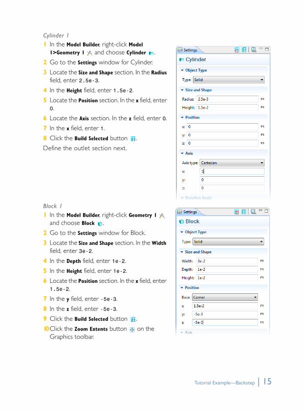
Cylinder 11 In the Model Builder, right-click Model
1>Geometry 1 and choose Cylinder .
2 Go to the Settings window for Cylinder.
3 Locate the Size and Shape section. In the Radius field, enter 2.5e-3.
4 In the Height field, enter 1.5e-2.
5 Locate the Position section. In the x field, enter 0.
6 Locate the Axis section. In the z field, enter 0.
7 In the x field, enter 1.
8 Click the Build Selected button .
Define the outlet section next.
Block 11 In the Model Builder, right-click Geometry 1
and choose Block .
2 Go to the Settings window for Block.
3 Locate the Size and Shape section. In the Width field, enter 3e-2.
4 In the Depth field, enter 1e-2.
5 In the Height field, enter 1e-2.
6 Locate the Position section. In the x field, enter 1.5e-2.
7 In the y field, enter -5e-3.
8 In the z field, enter -5e-3.
9 Click the Build Selected button .
10Click the Zoom Extents button on the Graphics toolbar.
Tutorial Example—Backstep | 15
cfd_introduction.book Page 16 Friday, September 23, 2011 12:07 PM
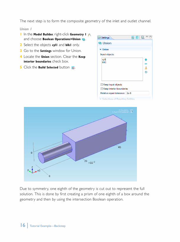
The next step is to form the composite geometry of the inlet and outlet channel.
Union 11 In the Model Builder, right-click Geometry 1
and choose Boolean Operations>Union .
2 Select the objects cyl1 and blk1 only.
3 Go to the Settings window for Union.
4 Locate the Union section. Clear the Keep interior boundaries check box.
5 Click the Build Selected button .
Due to symmetry, one eighth of the geometry is cut out to represent the full solution. This is done by first creating a prism of one eighth of a box around the geometry and then by using the intersection Boolean operation.
16 | Tutorial Example—Backstep
cfd_introduction.book Page 17 Friday, September 23, 2011 12:07 PM
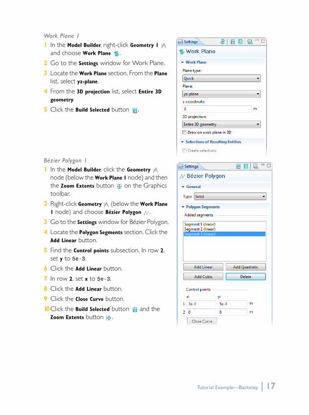
Work Plane 11 In the Model Builder, right-click Geometry 1
and choose Work Plane .
2 Go to the Settings window for Work Plane.
3 Locate the Work Plane section. From the Plane list, select yz-plane.
4 From the 3D projection list, select Entire 3D geometry.
5 Click the Build Selected button .
Bézier Polygon 11 In the Model Builder, click the Geometry
node (below the Work Plane 1 node) and then the Zoom Extents button on the Graphics toolbar.
2 Right-click Geometry (below the Work Plane 1 node) and choose Bézier Polygon .
3 Go to the Settings window for Bézier Polygon.
4 Locate the Polygon Segments section. Click the Add Linear button.
5 Find the Control points subsection. In row 2, set y to 5e-3.
6 Click the Add Linear button.
7 In row 2, set x to 5e-3.
8 Click the Add Linear button.
9 Click the Close Curve button.
10Click the Build Selected button and the Zoom Extents button .
Tutorial Example—Backstep | 17

cfd_introduction.book Page 18 Friday, September 23, 2011 12:07 PM
The triangle created, using the polygon tool, overlaps with one eighth of a fictive box around the geometry. This is used to create the prism for the intersection Boolean operation.
Extrude 11 In the Model Builder, right-click Work Plane 1
and choose Extrude .
2 Go to the Settings window for Extrude.
3 Locate the Distances from Work Plane section. In the table under Distances enter 4.5e-2.
4 Click the Build Selected button .
18 | Tutorial Example—Backstep
cfd_introduction.book Page 19 Friday, September 23, 2011 12:07 PM
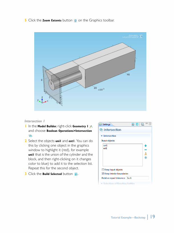
5 Click the Zoom Extents button on the Graphics toolbar.
Intersection 11 In the Model Builder, right-click Geometry 1
and choose Boolean Operations>Intersection .
2 Select the objects uni1 and ext1. You can do this by clicking one object in the graphics window to highlight it (red), for example uni1 that is the union of the cylinder and the block, and then right-clicking on it changes color to blue) to add it to the selection list. Repeat this for the second object.
3 Click the Build Selected button .
Tutorial Example—Backstep | 19
cfd_introduction.book Page 20 Friday, September 23, 2011 12:07 PM
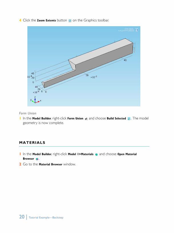
4 Click the Zoom Extents button on the Graphics toolbar.
Form Union1 In the Model Builder, right-click Form Union and choose Build Selected . The model
geometry is now complete.
MATERIALS
1 In the Model Builder, right-click Model 1>Materials and choose Open Material Browser .
2 Go to the Material Browser window.
20 | Tutorial Example—Backstep
cfd_introduction.book Page 21 Friday, September 23, 2011 12:07 PM
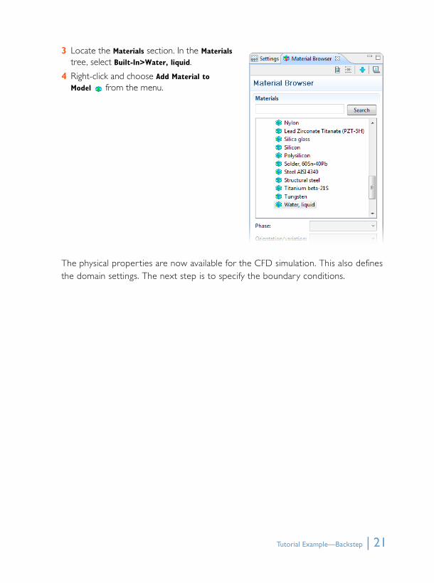
3 Locate the Materials section. In the Materials tree, select Built-In>Water, liquid.
4 Right-click and choose Add Material to Model from the menu.
The physical proper ties are now available for the CFD simulation. This also defines the domain settings. The next step is to specify the boundary conditions.
Tutorial Example—Backstep | 21

cfd_introduction.book Page 22 Friday, September 23, 2011 12:07 PM
LAMINAR FLOW
Inlet 11 In the Model Builder, right-click Model
1>Laminar Flow and choose Inlet .
2 Select Boundary 1 only, which represents the inlet.
3 Go to the Settings window for Inlet.
4 Locate the Boundary Condition section. From the Boundary condition list, select Laminar inflow.
5 Locate the Laminar Inflow section. In the Uav field, enter v0 (previously defined as a Global Parameter).
Symmetry 11 In the Model Builder, right-click Laminar Flow
and choose Symmetry .
2 Select Boundaries 2 and 3 only.
Outlet 11 In the Model Builder, right-click Laminar Flow
and choose Outlet .
The default outlet condition specifies a zero relative pressure.
2 Select Boundary 7 only.
All other boundaries have now the default wall condition.
22 | Tutorial Example—Backstep

cfd_introduction.book Page 23 Friday, September 23, 2011 12:07 PM
MESH 1
1 In the Model Builder, click Model 1>Mesh 1 .
2 Go to the Settings window for Mesh.
3 Locate the Mesh Settings section. From the Element size list, select Coarse.
The physics induced mesh will automatically introduce a mesh that is a bit finer on the walls compared to the free stream mesh. The close-up figure below shows the boundary layer mesh at the walls.
4 Click the Build All button .
STUDY 1
1 In the Model Builder, right-click Study 1 and choose Compute .
When Compute is selected, COMSOL automatically uses a suitable solver for the problem.
Tutorial Example—Backstep | 23

cfd_introduction.book Page 24 Friday, September 23, 2011 12:07 PM
RESULTS
Two plots are automatically created, one slice plot for the velocity and one pressure contour plot on the wall.
Velocity (spf)1 In the Model Builder, expand the Velocity (spf) node.
2 Right-click Slice 1 and choose Delete.
3 Click Yes to confirm.
4 In the Model Builder, right-click Velocity (spf) and choose Surface .
5 Right-click Velocity (spf) and choose Arrow Surface .
6 Go to the Settings window for Arrow Surface.
7 Locate the Coloring and Style section. From the Arrow length list, select Logarithmic.
8 From the Color list, select Yellow.
9 Click the Zoom Extents button on the Graphics toolbar.
To see the recirculation effects, create a streamline plot of the velocity field.
3D Plot Group 31 In the Model Builder, right-click Results and choose 3D Plot Group .
2 Right-click Results>3D Plot Group 3 and choose Streamline .
24 | Tutorial Example—Backstep
cfd_introduction.book Page 25 Friday, September 23, 2011 12:07 PM
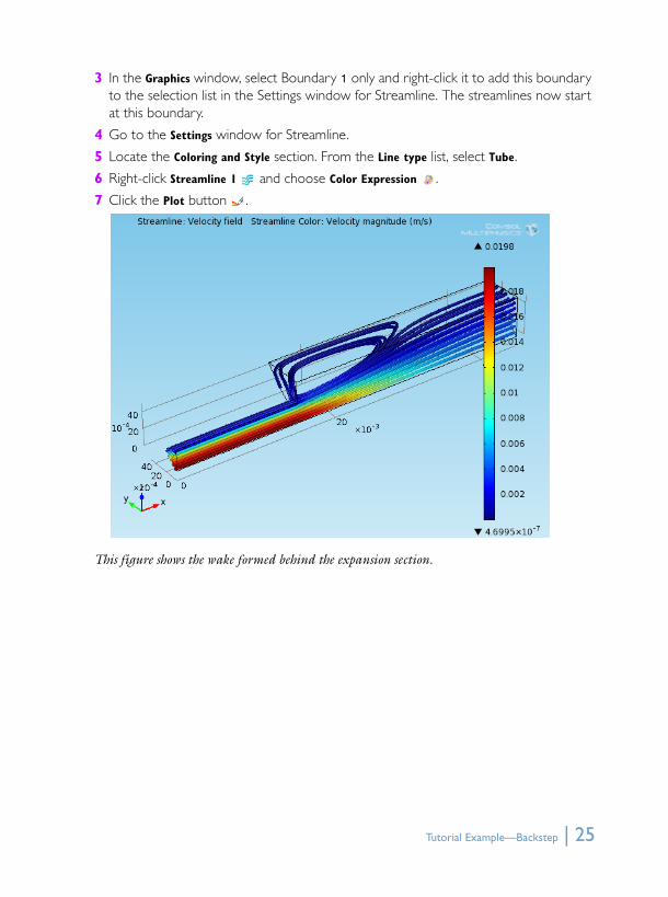
3 In the Graphics window, select Boundary 1 only and right-click it to add this boundary to the selection list in the Settings window for Streamline. The streamlines now start at this boundary.
4 Go to the Settings window for Streamline.
5 Locate the Coloring and Style section. From the Line type list, select Tube.
6 Right-click Streamline 1 and choose Color Expression .
7 Click the Plot button .
This figure shows the wake formed behind the expansion section.
Tutorial Example—Backstep | 25

cfd_introduction.book Page 26 Friday, September 23, 2011 12:07 PM
Tutorial Example—Heat SinkThis model is intended as an introduction to simulations of fluid flow and conjugate heat transfer. It demonstrates the following important points. How to:
• Draw an air box around a device in order to model convective cooling in this box.
• Set a total heat flux on a boundary using automatic area computation.
• Display results in an efficient way using selections in data sets.
The modeled system consists of an aluminum heat sink for cooling of components in electronic circuits mounted inside a channel of rectangular cross section (see the figure below). Such a set-up is used to measure the cooling capacity of heat sinks. Air enters the channel at the inlet and exits the channel at the outlet. The base surface of the heat sink receives a 1 W heat flux from an external heat source. All other external faces are thermally insulated.
The model set-up including channel and heat sink.
The cooling capacity of the heat sink can be determined by monitoring the temperature of the base surface of the heat sink.
The model solves a thermal balance for the heat sink and the air flowing in the rectangular channel. Thermal energy is transported through conduction in the aluminum heat sink and through conduction and convection in the cooling air. The
inlet
outlet base surface
26 | Tutorial Example—Heat Sink
cfd_introduction.book Page 27 Friday, September 23, 2011 12:07 PM
temperature field is continuous across the internal surfaces between the heat sink and the air in the channel. The temperature is set at the inlet of the channel. The base of the heat sink receives a 1W heat flux. The transport of thermal energy at the outlet is dominated by convection.
The flow field is obtained by solving one momentum balance for each space coordinate (x, y, and z) and a mass balance. The inlet velocity is defined by a parabolic velocity profile for fully developed laminar flow. At the outlet, a constant pressure is combined with the assumption that there are no viscous stresses in the direction perpendicular to the outlet. At all solid surfaces, the velocity is set to zero in all three spatial directions.
The thermal conductivity of air, the heat capacity of air, and the air density are all temperature-dependent material properties.
You can find all of the settings mentioned above in the physics interface for Conjugate Heat Transfer in COMSOL Multiphysics. You also find the material properties, including their temperature dependence, in the Material Browser.
Tutorial Example—Heat Sink | 27

cfd_introduction.book Page 28 Friday, September 23, 2011 12:07 PM
ResultsThe hot wake behind the heat sink visible in the figure below is a sign of the convective cooling effects. The maximum temperature, reached at the heat sink base, is slightly more than 375K.
The surface plot shows the temperature field on the channel walls and the heat sink surface, while the arrow plot shows the flow velocity field around the heat sink.
MODEL WIZARD
1 Go to the Model Wizard window.
2 Click Next to create a 3D model.
3 In the Add physics tree, select Heat Transfer>Conjugate Heat Transfer >Laminar Flow (nitf) .
4 Click Next .
5 In the Studies tree, select Preset Studies>Stationary .
6 Click Finish .
28 | Tutorial Example—Heat Sink

cfd_introduction.book Page 29 Friday, September 23, 2011 12:07 PM
GLOBAL DEFINITIONS
Parameters1 In the Model Builder, right-click Global Definitions and choose Parameters .
Define some parameters that are used when specifying the channel dimensions.
2 Go to the Settings window for Parameters.
3 Locate the Parameters section. In the Parameters table, enter the following settings:
NAME EXPRESSION DESCRIPTION
L_channel 7[cm] Channel length
W_channel 3[cm] Channel width
H_channel 1.5[cm] Channel height
U0 5[cm/s] Mean inlet velocity
Tutorial Example—Heat Sink | 29
cfd_introduction.book Page 30 Friday, September 23, 2011 12:07 PM
GEOMETRY 1
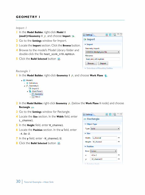
Import 1 1 In the Model Builder, right-click Model 1
(mod1)>Geometry 1 and choose Import .
2 Go to the Settings window for Import.
3 Locate the Import section. Click the Browse button.
4 Browse to the model’s Model Library folder and double-click the file heat_sink_n19.mphbin.
5 Click the Build Selected button .
Rectangle 1 1 In the Model Builder, right-click Geometry 1 and choose Work Plane .
2 In the Model Builder, right-click Geometry (below the Work Plane 1 node) and choose Rectangle .
3 Go to the Settings window for Rectangle.
4 Locate the Size section. In the Width field, enter L_channel.
5 In the Height field, enter W_channel.
6 Locate the Position section. In the x field, enter -4.5e-2.
7 In the y field, enter -W_channel/2.
8 Click the Build Selected button .
30 | Tutorial Example—Heat Sink

cfd_introduction.book Page 31 Friday, September 23, 2011 12:07 PM
Extrude 1 1 In the Model Builder, right-click Work Plane 1 (wp1)
and choose Extrude .
2 Go to the Settings window for Extrude.
3 Locate the Distances from Work Plane section. In the table under Distances enter H_channel.
4 Click the Build Selected button .
5 Click the Go to Default 3D View button on the Graphics toolbar.
6 Click the WireFrame Rendering button on the Graphics toolbar.
MATERIALS
1 In the Model Builder, right-click Model 1 (mod1)>Materials and choose Open Material Browser .
2 Go to the Material Browser window.
3 Locate the Materials section. In the Materials tree, select Built-In>Air.
4 Right-click and choose Add Material to Model from the menu.
AirBy default, the first material added applies to all domains. Typically, you can leave this setting and add other materials that override the default material where applicable. In this example, specify aluminum for Domain 2:
Tutorial Example—Heat Sink | 31
cfd_introduction.book Page 32 Friday, September 23, 2011 12:07 PM
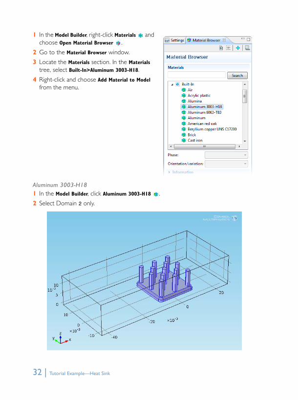
1 In the Model Builder, right-click Materials and choose Open Material Browser .
2 Go to the Material Browser window.
3 Locate the Materials section. In the Materials tree, select Built-In>Aluminum 3003-H18.
4 Right-click and choose Add Material to Model from the menu.
Aluminum 3003-H181 In the Model Builder, click Aluminum 3003-H18 .
2 Select Domain 2 only.
32 | Tutorial Example—Heat Sink

cfd_introduction.book Page 33 Friday, September 23, 2011 12:07 PM
CONJUGATE HEAT TRANSFER (NITF)
Fluid 11 In the Model Builder, right-click Model 1 (mod1)>Conjugate Heat Transfer (nitf) and
choose Fluid .
2 Select Domain 1 only.
Inlet 11 In the Model Builder, right-click Conjugate Heat
Transfer (nitf) and choose the boundary condition Laminar Flow>Inlet .
2 Select Boundary 115 only.
3 Go to the Settings window for Inlet.
4 Locate the Boundary Condition section. From the Boundary condition list, select Laminar inflow.
5 Locate the Laminar Inflow section. In the Uav field, enter U0.
Outlet 11 In the Model Builder, right-click Conjugate Heat
Transfer (nitf) and choose the boundary condition Laminar Flow>Outlet .
2 Select Boundary 1 only.
Tutorial Example—Heat Sink | 33
cfd_introduction.book Page 34 Friday, September 23, 2011 12:07 PM
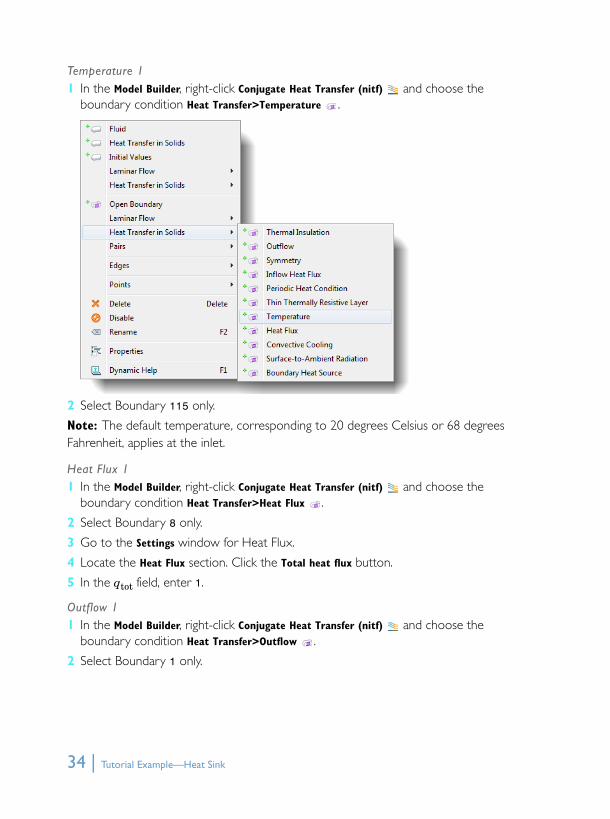
Temperature 11 In the Model Builder, right-click Conjugate Heat Transfer (nitf) and choose the
boundary condition Heat Transfer>Temperature .
2 Select Boundary 115 only.
Note: The default temperature, corresponding to 20 degrees Celsius or 68 degrees Fahrenheit, applies at the inlet.
Heat Flux 11 In the Model Builder, right-click Conjugate Heat Transfer (nitf) and choose the
boundary condition Heat Transfer>Heat Flux .
2 Select Boundary 8 only.
3 Go to the Settings window for Heat Flux.
4 Locate the Heat Flux section. Click the Total heat flux button.
5 In the qtot field, enter 1.
Outflow 11 In the Model Builder, right-click Conjugate Heat Transfer (nitf) and choose the
boundary condition Heat Transfer>Outflow .
2 Select Boundary 1 only.
34 | Tutorial Example—Heat Sink

cfd_introduction.book Page 35 Friday, September 23, 2011 12:07 PM
MESH 1
Free Tetrahedral 11 In the Model Builder, right-click Model 1 (mod1)>Mesh 1 and choose Free
Tetrahedral .
Size 11 In the Model Builder, right-click Free Tetrahedral 1
and choose Size .
2 Go to the Settings window for Size.
3 Locate the Geometric Entity Selection section. From the Geometric entity level list, select Domain.
4 Select Domain 1 only.
5 Locate the Element Size section. From the Predefined list, select Finer.
6 Click the Build All button .
STUDY 1
1 In the Model Builder, right-click Study 1 and choose Compute .
To reproduce the figures shown later in the Results section, define a selection of walls used for analysis.
Tutorial Example—Heat Sink | 35

cfd_introduction.book Page 36 Friday, September 23, 2011 12:07 PM
DEFINITIONS
In order to get a better plot, create a selection under the Definitions node.
Walls1 In the Model Builder, right-click Model 1 (mod1)>Definitions and choose
Selections>Explicit .
2 Go to the Settings window for Explicit.
3 Locate the Input Entities section. From the Geometric entity level list, select Boundary.
4 Right-click Explicit 1 and choose Rename.
5 Go to the Rename Explicit dialog box and enter walls in the New name field.
6 Click OK.
7 Select Boundaries 3 and 5–114 only.
36 | Tutorial Example—Heat Sink

cfd_introduction.book Page 37 Friday, September 23, 2011 12:07 PM
RESULTS
Data Sets1 In the Model Builder, expand the Data Sets node . Right-click Results>Data
Sets>Solution 1 and choose Add Selection .
2 Go to the Settings window for Selection.
3 Locate the Geometric Entity Selection section. From the Geometric entity level list, select Boundary.
4 From the Selection list, select walls.
Temperature (nitf)1 In the Model Builder, click Results>Temperature (nitf) .
2 Go to the Settings window for 3D Plot Group.
3 Locate the Data section. From the Data set list, select Solution 1.
4 Right-click Results>Temperature (nitf) and choose Arrow Volume .
5 Go to the Settings window for Arrow Volume.
6 In the upper-right corner of the Expression section, click Replace Expression.
Tutorial Example—Heat Sink | 37
cfd_introduction.book Page 38 Friday, September 23, 2011 12:07 PM
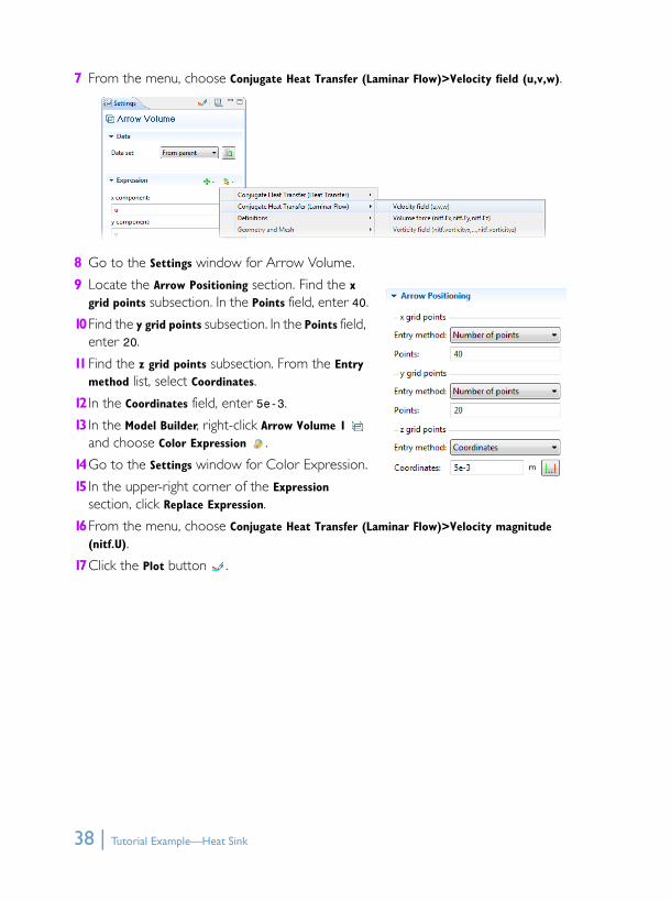
7 From the menu, choose Conjugate Heat Transfer (Laminar Flow)>Velocity field (u,v,w).
8 Go to the Settings window for Arrow Volume.
9 Locate the Arrow Positioning section. Find the x grid points subsection. In the Points field, enter 40.
10Find the y grid points subsection. In the Points field, enter 20.
11Find the z grid points subsection. From the Entry method list, select Coordinates.
12 In the Coordinates field, enter 5e-3.
13 In the Model Builder, right-click Arrow Volume 1 and choose Color Expression .
14Go to the Settings window for Color Expression.
15 In the upper-right corner of the Expression section, click Replace Expression.
16From the menu, choose Conjugate Heat Transfer (Laminar Flow)>Velocity magnitude (nitf.U).
17Click the Plot button .
38 | Tutorial Example—Heat Sink

cfd_introduction.book Page 4 Friday, September 23, 2011 12:07 PM

www.comsol.comCM021302