Jacobi last multiplier, Lie symmetries, andhidden linearity: what’s up

M C NucciDipartimento di Matematica e Informatica,Universita di Perugia, 06123 Perugia, Italy

E-mail: nucci@unipg.it

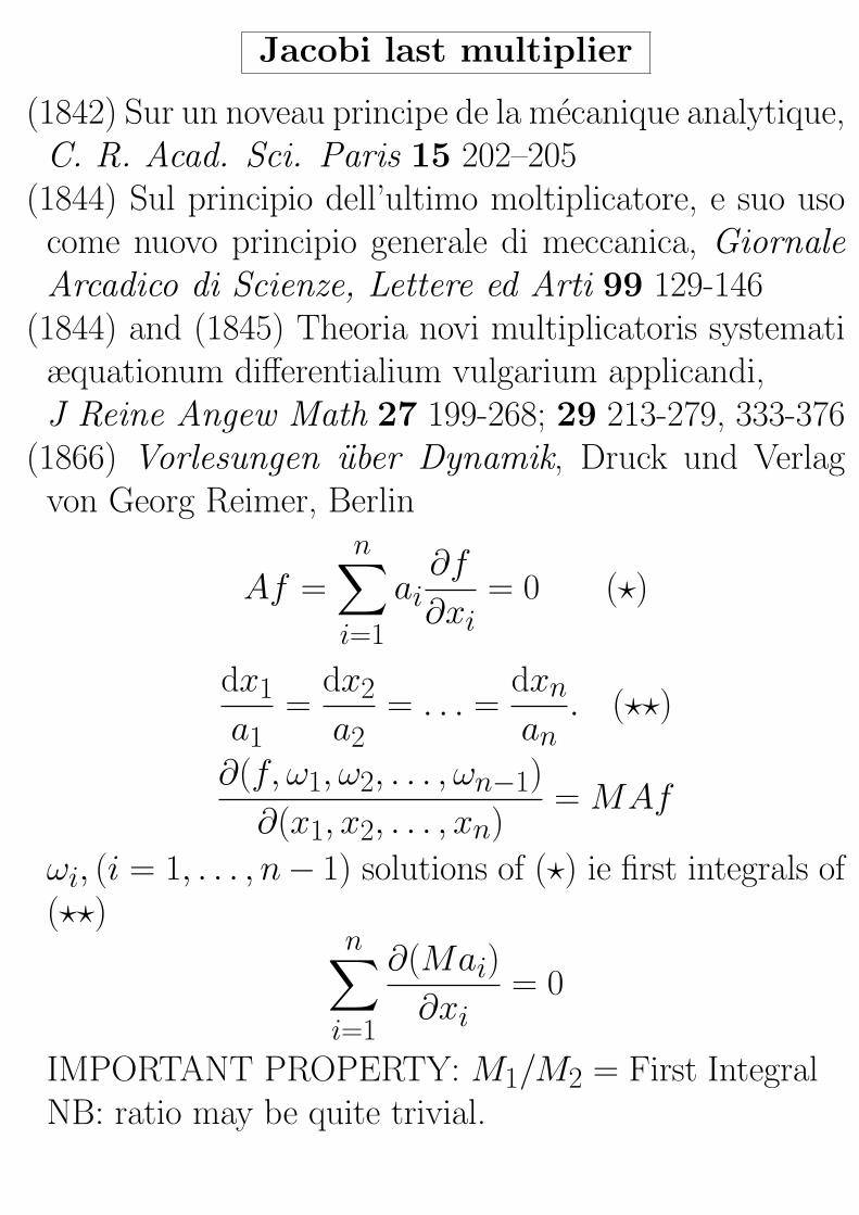
Jacobi last multiplier

(1842) Sur un noveau principe de la mecanique analytique,C. R. Acad. Sci. Paris 15 202–205

(1844) Sul principio dell’ultimo moltiplicatore, e suo usocome nuovo principio generale di meccanica, GiornaleArcadico di Scienze, Lettere ed Arti 99 129-146

(1844) and (1845) Theoria novi multiplicatoris systematiæquationum differentialium vulgarium applicandi,J Reine Angew Math 27 199-268; 29 213-279, 333-376

(1866) Vorlesungen uber Dynamik, Druck und Verlagvon Georg Reimer, Berlin

Af =

n∑

i=1

ai∂f

∂xi= 0 (?)

dx1

a1=

dx2

a2= . . . =

dxn

an. (??)

∂(f, ω1, ω2, . . . , ωn−1)

∂(x1, x2, . . . , xn)= MAf

ωi, (i = 1, . . . , n− 1) solutions of (?) ie first integrals of(??)

n∑

i=1

∂(Mai)

∂xi= 0

IMPORTANT PROPERTY: M1/M2 = First IntegralNB: ratio may be quite trivial.

JLM and Lie symmetries

Lie S (1874) Veralgemeinerung und neue Verwerthungder Jacobischen Multiplicator-Theorie, Fordhandlingeri Videnokabs –Selshabet i Christiania 198-226

Lie S (1912) Vorlesungen uber Differentialgleichun-gen mit Bekannten Infinitesimalen Transformatio-nen, Teubner, Leipzig

Bianchi L (1918) Lezioni sulla teoria dei gruppi con-tinui finiti di trasformazioni, Enrico Spoerri, PisaIf there exist n− 1 symmetries of

dx1

a1=

dx2

a2= . . . =

dxn

an.

sayΓi = ξij∂xj, i = 1, n− 1

then JLM is given by M = ∆−1, provided that ∆ 6= 0,where

∆ = det

a1 · · · an

ξ1,1 ξ1,n... ...

ξn−1,1 · · · ξn−1,n

Corollary: if ∃ M=const, then ∆ is a first integral.The equation for JLM is

d log(M)

dt= −

n∑

i=1

∂ai

∂xi

If ∂ai/∂xi = 0 ⇒ M=const.

A novel approach

Lie group analysis: the most powerful tool to findthe general solution of ODEs.

Major drawback of Lie’s method: useless when appliedto systems of first-order ODEs.Ansatz? when successful (rarely!) it is just a lucky guess.

[MCN, 1996]: the technique of reduction/increasingof order. Successfully applied in several instances [Tor-risi V and MCN (2001), MCN and Leach PGL (2001),Marcelli M and MCN (2003), MCN (2003), MCN andLeach PGL (2004), MCN (2004), MCN (2005), EdwardsM and MCN (2006), Gradassi A and MCN (2006)].

Here we show that if we increase the order (also after areduction of order) by using Jacobi last multiplier, thenwe may found enough Lie point symmetries that enableus to integrate the original equation a la Lie.

An equation from Kamke

[Kamke E (1883), Ch 6, 542ff]

y′′ =y′2y

+ f ′(x)yp+1 + pf (x)y′yp, (1)

where p 6= 0 is a real constant and f 6= 0 is an arbi-trary function of the independent variable x. It does notpossess Lie point symmetries for general f (x) and yet istrivially integrable [Gonzalez-Lopez A (1988)].We transform (1) into:

w′1 = w2,

w′2 =1

w1(w

p+21 f ′ + w2

2 + wp+11 w2fp) (2)

(w1 = y and w2 = y′) The Jacobi last multiplier of thissystem satisfies:

d log(M)

dx+ pw

p1f + 2

w2

w1= 0

which suggests the transformation

w2 = w1r′2 − pw

p1f

2.

NB: just a point transformation between r2 and M .Then system (2) transforms into:

w′1 =w1

2(r′2 − w

p1fp),

r′′2 =w

p1

2

((r′2 − w

p1fp

)fp + 2f ′

)(p + 2) (3)

Lie operator:

Γ = V (x,w1, r2)∂x+G1(x,w1, r2)∂w1+G2(x,w1, r2)∂r2

Lie group analysis =⇒ determining equation for V [Mar-celli and MCN, (2003)]

Its characteristic curve w1e−r2/2 =⇒ w1 = r1e

r2/2.Then, system (3) transforms into:

r′1 = −1

2

(e

r22 r1

)pfpr1,

r′′2 =

(e

r22 r1

)p

2

(2pf ′ + 4f ′ −

(e

r22 r1

)p(p + 2)f2p2

+pf (p + 2)r′2), (4)

which admits a two-dimensional Lie symmetry algebraL2 generated by

Γ1 = r1∂r1 − 2∂r2, Γ2 =1

r1∂r1 −

2(p + 2)

pr21

∂r2.

A basis of differential invariants of L2 of order ≤ 1:

x = x, u = r′2 − (2 + p)pfrp1e

pr22 . (5)

Then (4) is reduced to:

du

dx= 0 =⇒ u = a1 (6)

Then (5) yields

r1 = e−r22

(r′2 − a1

f (p + 2)

)1p

. (7)

Finally, we have to solve:

r′′2 = −(a1 − r′2)(a1p + 2r′2)pf − 2(p + 2)f ′

2(p + 2)f, (8)

⇒ non-abelian intransitive L2 generated by

X1 = ∂r2, X2 = epr2−a1x

p+2 ∂r2.

TYPE IV [Lie 1883] Canonical form:

∂r2, r2∂r2

⇒ x = x, r2 = −p + 2

pe

pp+2(a1x−r2)

and equation (8) becomes

d2r2

dx2=

dr2

dx

2f ′ + a1pf

2f

After two quadratures the general solution is obtained

r2 = a2

∫fe

a1px2 dx + a3

and consequently the general solution of (8) is

r2 = −(p+2) log

(− p

p + 2

(a2

∫e

a1px2 f dx− a3

))+a1x.

Finally the general solution of equation (1) is

y = w1 = r1er2/2 = e

xa12

(−p

∫e

xa1p2 f dy + a2p

)−1p

with a2 = −a3/a2.

A linearizable equation given by Painleve

An example of an equation which does not possess thePainleve property [Painleve (1900), Ince (1956)]:

w′′ = w′2wλ(2k2w2 − 1− k2)−√

(1− w2)(1− k2w2)

(1− w2)(1− k2w2)

Case k = 1 (after a cosmetic rescaling u = w/λ):

u′′ = u′2 2u + 1

u2 − λ2(9)

Calogero (2002) showed that it features many periodicsolutions and that all of its nonsingular solutions areperiodic. We note that Eq (1) admits sl(3, IR):

X1 = −(

u + λ

u− λ

) 12λ

[x ∂x + (λ2 − u2) ∂u]

X2 = −(

u + λ

u− λ

) 12λ

∂x

X3 =

(u− λ

u + λ

) 12λ

(u2 − λ2)x ∂u

X4 =

(u− λ

u + λ

) 12λ

(u2 − λ2) ∂u (10)

X5 = −x2∂x + x(u2 − λ2) ∂u

X6 = (u2 − λ2) ∂u

X7 = ∂x X8 = x∂x

It means that equation (9) is linearizable. We look for atwo-dimensional abelian intransitive subalgebra:

∂u, x∂u (Canonical form) (11)

i.e., < X2, X7 >

⇒ x =

(u− λ

u + λ

) 12λ

, u = x

(u− λ

u + λ

) 12λ

, (12)

and equation (9) becomes

d2u

dx2= 0. (13)

Its general solution is u = a1x + a2, which implies

(u− λ)12λ(x− a1)− (u + λ)

12λa2 = 0 (14)

Let’s remark that the transformation

z =1√

u2 + x2, τ = arctan

(−u

x

)

and viceversa

u =sin(τ )

z, x = −cos(τ )

z

takes the free particle equation (13) into a harmonic os-cillator, ie

d2z

dτ2+ z = 0.

In order to apply the method of Jacobi last multi-plier equation (9) is written as the system of two nonau-tonomous first-order ordinary differential equations:

u′ = ux,

u′x = u2x

2u + 1

u2 − λ2(15)

with ux a new obvious dependent variable. Constructthe first prolongations of the generators (10). For exam-ple the first prolongation of X1 is

X11

= X1 +

(u + λ

u− λ

) 12λ

uxxux + 2λ2u− 2u3

λ2 − u2∂ux

There are 28 possible determinants to be calculated.By way of illustration the matrix that we obtain withthe choice of X1

1and X3

1is

C13 =

1 ux u2x

2u + 1

u2 − λ2

−(

u + λ

u− λ

) 12λ

x

(u + λ

u− λ

) 12λ

(u2 − λ2)

(u + λ

u− λ

) 12λ

uxxux + 2λ2u− 2u3

λ2 − u2

0

(u− λ

u + λ

) 12λ

(u2 − λ2) x

(u− λ

u + λ

) 12λ

(2xuux + xux + u2 − λ2)

(16)

Using Maple 7 it is easy to find that the determinantswhich are different from zero are the following:

∆13 = (u2 − λ2 + xux)2

∆14 = (u2 − λ2 + xux)ux

∆15 =

(u + λ

u− λ

) 12λ (u2 − λ2 + xux)3

u2 − λ2

∆17 =

(u + λ

u− λ

) 12λ u2

x(u2 − λ2 + xux)

λ2 − u2

∆18 =

(u + λ

u− λ

) 12λ ux(u2 − λ2 + xux)2

λ2 − u2

∆23 = ∆14

∆24 = u2x

∆25 = ∆18

∆27 =

(u + λ

u− λ

) 12λ u3

x

λ2 − u2

∆28 = ∆17

∆34 = −(

u− λ

u + λ

)1λ

(λ2 − u2)2

∆36 =

(u− λ

u + λ

) 12λ

(λ2 − u2)(u2 − λ2 + xux)

∆37 = −(

u− λ

u + λ

) 12λ

(λ2 − u2)ux

∆45 = −(

u− λ

u + λ

) 12λ (

(λ2 − u2)xux − (u2 − λ2)2

+x2u2x1− λ2 + 2u + 2u2 + 2uλ2

1 + u2

)

∆46 = −∆37

∆47 =

(u− λ

u + λ

) 12λ

u2x1− λ2 + 2u + 2u2 + 2uλ2

1 + u2

The following are first integrals of system (15) and con-sequently of equation (9):

I1 =∆13

∆14=

u2 − λ2 + xux

ux

I2 =∆13

∆15=

(u− λ

u + λ

) 12λ λ2 − u2

u2 − λ2 + xux

I3 =∆13

∆17=

(u− λ

u + λ

) 12λ (λ2 − u2)(u2 − λ2 + xux)

u2x

=I21I2

I4 =∆13

∆18=

(u− λ

u + λ

) 12λ λ2 − u2

ux= I1I2

I5 =∆14

∆15= −I1

I2

I6 =∆14

∆17= I2

I7 =∆14

∆18=

∆13

∆15= I2

I9 =∆15

∆17= −I2

1 .

Naturally we have omitted all the other possible combi-nations (seventy-eight in total).

Calogero’s goldfish

Case N=4

z1 = 2

(z1z2

z1 − z2+

z1z3

z1 − z3+

z1z4

z1 − z4

)

z2 = 2

(z2z1

z2 − z1+

z2z3

z2 − z3+

z2z4

z2 − z4

)(17)

z3 = 2

(z3z1

z3 − z1+

z3z2

z3 − z2+

z3z4

z3 − z4

)

z4 = 2

(z4z1

z4 − z1+

z4z2

z4 − z2+

z4z3

z4 − z3

)

z1 = w1, z2 = w2, z3 = w3, z4 = w4, z1 = w5, z2 =w6, z3 = w7, z4 = w8 ⇒ autonomous system of 8 equa-tions of first ordery = w1 ⇒ non-autonomous system of 7 equations offirst order. Eliminating w6, w7, w8, i.e. w6 = w′2w5,w7 = w′3w5, w8 = w′4w5 yields

w′5 = −2w5((w3 − y)(w2 − y)w′4+(w4 − y)(w2 − y)w′3+(w3 − y)(w4 − y)w′2)/((w2 − y)(w3

−y)(w4 − y))

w2 ≡ u2, w3 ≡ u3, w4 ≡ u1u′′1 = 2(((u2

3 − u3y − u′3y2 + (2u3 + y)(u3 − y)u′2)y + ((2u′3 + 1)y − u3)u

22

−((u3 − 2y)u3 + (u′3 + 1)y2)u2 − (u2 + u3)(u2 − y)(u3 − y)u′1)u1

+((u2 − y)u′3 + (u3 − y)u′2)u31 + (u2 − y)(u3 − y)u′1u2u3

+(u2 − y)(u23 − u3y − u′3y

2)u2 − (u3 − y)u′2u3y2 + (((2u′3 + 1)y − u3)y

−u22u′3 − (u3 + 2y)(u3 − y)u′2 − ((u′3 + 1)y − u3)u2

+(u2 − y)(u3 − y)u′1)u21)u

′1/((u1 − u2)(u1 − u3)(u1 − y)(u2 − y)(u3 − y))

u′′2 = (−2((u2 − u3)(u2 − y)2(u3 − y)u′1 − u32u′3y + (u2

2u′3 + u2u

′2u3 − u2u

′2y

+u2u3 − 2u2u′3y − u2y − u′2u

23 + u′2u3y − u2

3 + u3y + u′3y2)(u2 + y)u1 (18)

+(u23 − u3y − u′3y

2 + (u3 − y)u′2u3)u2y + ((2u′3 + 1)y − u3 − (u3 − y)u′2)u22y

+((u3 − y)u′2u3 − u22u′3 + u2

3 − u3y − u′3y2 + ((2u′3 + 1)y − u3

−(u3 − y)u′2)u2)u21)u

′2)/((u1 − u2)(u1 − y)(u2 − u3)(u2 − y)(u3 − y))

u′′3 = (2(((u22 + u3y)(u′3 + 1)− (u3 − y)2u′2 − (u3 + y)(u′3 + 1)u2)u3y

−(u2 − u3)(u2 − y)(u3 − y)2u′1 + (((u3 + y)u2 − u3y)(u′3 + 1) + (u3 − y)2u′2−(u′3 + 1)u2

2)(u3 + y)u1 + ((u22 + u3y)(u′3 + 1)− (u3 − y)2u′2

−(u3 + y)(u′3 + 1)u2)u21)u

′3)/((u1 − u3)(u1 − y)(u2 − u3)(u2 − y)(u3 − y))

Lie group analysis ⇒ L24 iso sl(5, IR)⇒ linearizable by means of the following transformation

y = y + u1 + u2 + u3 = z1 + z2 + z3 + z4

u1 = yu1u2u3 = z1z2z3z4

u2 = yu1u2 + yu1u3 + yu2u3 + u1u2u3

= z1z2z3 + z1z2z4 + z1z3z4 + z2z3z4 (19)

u3 = yu1 + yu2 + yu3 + u1u2 + u1u3 + u2u3

= z1z2 + z1z3 + z1z4 + z2z3 + z2z4 + z3z4

System (18) becomes

d2uk

dy2= 0, k = 1, 2, 3 (20)

equations of one-dimensional motion of three free-particles.

Hidden linearity

• Jacobi modular equation ⇒ sl(2, IR)⇒ free-particle equation

• Calogero’s goldfish (n ODEs) ⇒ sl(n + 1, IR)⇒ free-particle equations

• Jacobi’s three-body system ⇒ sl(2, IR)n 2A1⇒ free-particle equation

• multi-species Lotka-Volterra model ⇒ sl(3, IR)⇒ free-particle equation

Separation of variables ⇒ free-particle equations

Periodic solutions ⇒ free-particle equation(s) ?

Final remarks

Lie group analysis should still be considered an essen-tial tool for anyone who wants to “compete” with equa-tions of relevance in physics and other scientific fields.

As brilliantly stated by Ibragimov (1991):

cherchez le groupe!

However Jacobi docet:

Mathematics cannot invent the laws of nature.Wherever Mathematics is mixed up with any-thing, which is outside its field, you will findattempts to demonstrate these merely propo-sitions a priori, and it will be your task tofind out the false deduction in each case.

[Jacobi CGJ, Vorlesungen uber Analytische

Mechanik (1847-1848)]

[Pulte H, Historia Math. 25 (1998), 154-184.]

AN INTEGRABLE NONLINEAR EVOLUTIONEQUATION IN 3+1 DIMENSIONS?????

ηt = η3ηzzz + 3η2ηxzz + 3η2ηyz + 3η2ηyzzz

+3η2ηzηzz + 3ηηxηzz + 3ηηxxz + 3ηηxy + 6ηηxyzz

+3ηηxzηz + 3ηηyηzzz + 3ηηyyz + 3ηηyyzz2 + 3ηηyzηzz

−36ηyz + 3ηxηxz + 3ηxηyzz − 6ηxy2 + ηxxx + 3ηxxyz

+3ηxyyz2+3ηxzηyz+3ηyηyzz

2+ηyyyz3+12ηzyz2−12z3

AN INTEGRABLE NONLINEAR EVOLUTIONEQUATION IN 4+1 DIMENSIONS?????

Ωt = 6ΩxwzΩz + 3ΩxxzΩ + 3ΩxzΩzΩ + 3ΩxzΩx

+3ΩxzΩyw + 3ΩxzΩwz + 6ΩywzΩzw + 3ΩyyzΩw2

+3ΩyzΩzΩw + 3ΩyzΩxw + 3ΩyzΩyw2 + 3ΩyzΩwzw

+3ΩyzΩz + 3ΩwwzΩz2 + 3ΩwzΩzΩz + 3ΩwzΩxz

+3ΩwzΩyzw + 3ΩwzΩwz2 + 3ΩwzΩ2 + ΩzzzΩ

3

+3ΩxzzΩ2 + 3ΩyzzΩ

2w + 3ΩwzzΩ2z + 3ΩzzΩzΩ

2

+3ΩzzΩxΩ + 3ΩzzΩyΩw + 3ΩzzΩwΩz + 36Ωzzyw

+12Ωzw3 + 6Ωxywzw + 3Ωxyyw

2 + 3Ωxyz + 3Ωxwwz2

+3ΩxwΩ+Ωxxx+3Ωxxyw+3Ωxxwz−6Ωxy2+3Ωywwz2w

+3ΩywΩw + 3Ωywz2 + Ωyyyw3 + 3Ωyywzw2 + 3Ωyyzw

+Ωwwwz3 +6ΩxyzΩw +3ΩwwΩz +12Ωwyw2− 48Ωyw

−36z2y − 72zw2

Some References

MCN, “Calogero’s “goldfish” is indeed a school of free particles” J.Phys. A: Math. Gen. 37 (2004), 11391-11400.

MCN, “Jacobi’s three-body system moves like a free particle” J. Non-linear Math. Phys. 12-s1 (2005) 499-506.

MCN, “Let’s Lie: a miraculous haul of fishes” Theor. Math. Phys.144 (2005) 1214-1222.

L. Rosati and MCN, “A Lie symmetry connection between Jacobi’smodular differential equation and Schwarzian differential equation”J. Nonlinear Math. Phys. 12 (2005) pp. 144–161.

MCN, “Jacobi last multiplier and Lie symmetries: a novel applica-tion of an old relationship” J. Nonlinear Math. Phys. 12 (2005)284-304.

MCN and P.G.L. Leach, “Jacobi’s last multiplier and the completesymmetry group of the Ermakov-Pinney equation” J. NonlinearMath. Phys. 12 (2005) pp. 305–320.

M. Edwards and MCN, “Application of Lie group analysis to a coregroup model for sexually transmitted diseases”, J. Nonlinear Math.Phys. (2006) to appear.

A. Gradassi and MCN, “Hidden linearity in systems for competitionwith evolution in ecology and finance”, (2006) to be submitted

A. Gradassi and MCN, “Integrability in a variant of the three-speciesLotka-Volterra model” (2006) to be submitted

E. Conti and MCN, “Euler’s multipliers and Lie symmetries” (2006)to be submitted

Work on JLM in different contexts

Since Lie’s work:

• searching for its generalization [De Donder];

• exploiting all the possible relationships it has with first integralsand Lie symmetries [Chella], [Saltykow];

• determining a Lagrangian formulation for systems of second-order ordinary differential equations [Whittaker], [MadhavaRao],[Jones & Vujanovic];

• searching for steady compressible flows of perfect gases [Opa-towski];

• applying it to the statistical mechanics of dissipative systems[Deshpande];

• identifying its analogue in QM (time-dependent probability den-sity) [KrishnaRao];

• relating its inverse to limit cycles [Berrone & Giacomini];

• finding first integrals of various systems [Grammaticos et al],[Roman-Miller & Broabridge], [MCN & Leach];

• deducing local [MCN] and nonlocal Lie symmetries [MCN &Leach].

References

Berrone L R and Giacomini H, Inverse Jacobi multipliers, Rend.Circ. Mat. Palermo Serie II 52 (2003), 77–130.

Chella T, Vantaggi che si possono trarre da noti invarianti integralie differenziali in alcuni problemi di integrazione, Ann. R. ScuolaNormale Sup. Pisa Sc. Fis. Mat. Nat. 11 (1910), 9–137.

De Donder T, Sur le multiplicateur de Jacobi generalise, Bull. del’Acad. Roy. de Belgique, Cl. de Sciences (1908), 795–811.

Deshpande S M, The averaging principle and the diagram technique,Physica A 80 (1975), 287–299.

Grammaticos B, Moulin Ollagnier J, Ramani A, Strelcyn J M andWojciechowski S, Integrals of quadratic ordinary differential equa-tions in R3: the Lotka-Volterra system, Physica A 163 (1990),683–722.

Jones S E and Vujanovic B, On the inverse Lagrangian problem, ActaMech. 73 (1988), 245–251.

Krishna Rao D, The last multiplier in quantum mechanics, J. MysoreUniv. Sect. B. 2 (1941), 1–4.

Laguerre E N, Application du principe du dernier multiplicateur al’integration d’une equation differentielle du second ordre, Bull.Sci. Math. Astron. 2 (1871), 246–250. Madhava Rao B S, Onthe reduction of dynamical equations to the Lagrangian form, Proc.Benares Math. Soc. 2 (1940), 53–59.

Opatowski I, Two-dimensional compressible flows, Proc. SymposiaAppl. Math. (A.M.S.) 1 (1949), 87–93.

Roman-Miller L and Broadbridge P, Exact integration of reducedFisher’s equation, reduced Blasius equation, and the Lorenz model,J. Math. Anal. Appl. 251 (2000), 65–83.

Saltykow N, Lie-ovo generalizanje teorije poslednjeg mnozitelja, Glas.Srpske Akad. Nauka. Od. Prirod.-Mat. Nauka 198 (1950), 1–16.

The method of the JLM provides a means to determine all thesolutions of the partial differential equation

Af =

n∑i=1

ai(x1, . . . , xn)∂f

∂xi= 0 (21)

or its equivalent associated Lagrange’s system

dx1

a1=

dx2

a2= . . . =

dxn

an. (22)

In fact, if one knows the JLM and all but one of the solutions, thenthe last solution can be obtained by a quadrature. The JLM M isgiven by

∂(f, ω1, ω2, . . . , ωn−1)

∂(x1, x2, . . . , xn)= MAf, (23)

where

∂(f, ω1, ω2, . . . , ωn−1)

∂(x1, x2, . . . , xn)= det

∂f

∂x1· · · ∂f

∂xn∂ω1

∂x1

∂ω1

∂xn... ...∂ωn−1

∂x1· · · ∂ωn−1

∂xn

= 0 (24)

and ω1, . . . , ωn−1 are n − 1 solutions of (21) or, equivalently, firstintegrals of (22) independent of each other.

Essential properties of the JLM

a) If one selects a different set of n − 1 independent solutionsη1, . . . , ηn−1 of equation (21), then the corresponding last mul-tiplier N is linked to M by the relationship:

N = M∂(η1, . . . , ηn−1)

∂(ω1, . . . , ωn−1).

b) Given a non-singular transformation of variables

τ : (x1, x2, . . . , xn) −→ (x′1, x′2, . . . , x

′n),

then the last multiplier M ′ of A′F = 0 is given by:

M ′ = M∂(x′1, x

′2, . . . , x

′n)

∂(x1, x2, . . . , xn),

where M obviously comes from the n− 1 solutions of AF = 0which correspond to those chosen for A′F = 0 through theinverse transformation τ−1.

c) One can prove that each multiplier M is a solution of thefollowing linear partial differential equation:

n∑i=1

∂(Mai)

∂xi= 0;

viceversa every solution M of this equation is a JLM.

d) If one knows two JLM M1 and M2 of equation (21), then theirratio is a solution ω of (21), or, equivalently, a first integral of(22). Naturally the ratio may be quite trivial, namely a constant.Viceversa the product of a multiplier M1 times any solution ωyields another last multiplier M2 = M1ω.

In its original formulation the method of the JLM required almostcomplete knowledge of the system, (21) or (22), under considera-tion. Since the existence of a solution/first integral is consequent

upon the existence of symmetry, an alternate formulation in termsof symmetries was provided by Lie. A clear treatment of the formu-lation in terms of solutions/first integrals and symmetries is givenby Bianchi. If we know n− 1 symmetries of (21)/(22), say

Γi =

n∑j=1

ξij(x1, . . . , xn)∂xj, i = 1, n− 1, (25)

Jacobi’s last multiplier is given by M = ∆−1, provided that ∆ 6= 0,where

∆ = det

a1 · · · an

ξ1,1 ξ1,n... ...

ξn−1,1 · · · ξn−1,n

. (26)

There is an obvious corollary to the results of Jacobi mentionedabove. In the case that there exists a constant multiplier, the de-terminant is a first integral. This result is potentially very usefulin the search for first integrals of systems of ordinary differentialequations. The differential equation to be solved for the JLM is

d log(M)

dt+

n∑i=1

∂Wi

∂wi= 0, (27)

where M is the multiplier and the equation of motion has compo-nents

wi = Wi(w1, . . . , wn) (28)

in which overdot denotes differentiation with respect to an indepen-dent variable, say t. Consequently, if each component of the vectorfield of the equation of motion is missing the variable associatedwith that component, i.e., ∂Wi/∂wi = 0, the last multiplier is aconstant. Note that equation (27) implies that the JLM M is equalto

M = exp

(−

∫ n∑i=1

∂Wi

∂widt

). (29)

If we assume that system (22) admits a Lie symmetry group gener-ated by the following operator:

Γ =

n∑i=1

ξi(x1, . . . , xn)∂xi, (30)

then Lie showed that a first integral of system (22) is given by:

Γ(log M) +

n∑i=1

(∂ξi

∂xi+ ξi

∂ log aj

∂xi− ai

aj

∂ξj

∂xi

)(31)

where j is any integer between 1 and n such that aj 6= 0. Lie’soriginal formula is actually:

Γ(log M) +

n∑i=1

∂ξi

∂xi+ λ

with [Γ,A] = λA as can be found on page 346 (Satz 12) of Lie’sfundamental book and also on page 464 of Bianchi’s book. In apaper published in 1992, Hojman claimed to have constructed a newconserved quantity for a dynamical system ql = αl(q, q, t) comingfrom the knowledge of an admitted Lie symmetry group E = ηl∂ql

+ηl∂ql

, namely

E(log M) +∂ηl

∂ql+

∂ηl

∂ql

which is obviously a particular case of Lie’s formula (31).Let us remark that the “generalizations” of the so-called Hojman’sresult, which were derived in [Gonzalez-Gascon 1994] and [Lutzky1995], are also included in Lie’s formula. Last but not least none ofthe cited authors seemed to know that M is the JLM.

MAI INFIRMARE IL DIRITTO DELLE LIBERE EMOLTEPLICI PROSPETTIVE INDIVIDUALI(NEVER INVALIDATE THE RIGHT OF FREE AND

MULTIPLE INDIVIDUAL PERSPECTIVES)GUIDO CALOGERO (July 25, 1961)

La competizione che conta, non e quella con gliuomini, bensı quella con le cose

(The competition which is worthy of consideration is not withmen, rather with objects.)

Guido Calogero (October 17, 1961)