l03 act pid

8/10/2019 L03 ACT PID

http://slidepdf.com/reader/full/l03-act-pid 1/62

Advanced Control Technology Club Advanced Control Technology Club(ACT Club)(ACT Club)

PID CONTROLPID CONTROL

Presentation provided by Dr Andy CleggPresentation provided by Dr Andy Clegg

8/10/2019 L03 ACT PID


Presentation OverviewPresentation OverviewIntroduction

PID parameterisation and structure

Effects of PID terms

Proportional, Integral and Derivative terms

Tuning PID Controllers

Equivalence of PID and Lead-Lag

controllers

Implementation aspects of PID

8/10/2019 L03 ACT PID


Introduction to PID ControlIntroduction to PID Control

Proportional-Integral-Derivative control

Predominant controller used in industry

Reason: it is adequate for most applications

Initially: analogue implementation

Now: mostly digital

8/10/2019 L03 ACT PID


Motivation and LimitationsMotivation and LimitationsMotivation

Simple to get working Can be tuned to meet time-domain specifications

Readily available in PLC/DCS systems

Digital and analogue implementation easy

Limitations

For single-input single-output systems only

Difficult to tune to meet precise specifications

Subtle differences in implementation causes problems

8/10/2019 L03 ACT PID


Idealised PIDIdealised PID--ControllerControllerConfigurationConfiguration

u(s)K(s)

r(s)

e(s)

y(s)PlantController

Set-Point Output

8/10/2019 L03 ACT PID


Generic PID Control EquationsGeneric PID Control Equations

Time domain:

Laplace domain:

However there are many different structures ...

D I

t

P

c dt

de

k dt t ek t ek t u 3

0

21 )()()( ++= ∫

D

s sE k

I

s E s

k s E k sU c )()()()( 3

2

P

1 ++=

8/10/2019 L03 ACT PID


““ IdealIdeal”” PID ParameterisationPID Parameterisation

K c: proportional coefficient

Ti: integral time constant

Td: derivative time constant

Common in PLC and DCS implementations

⎥⎥

⎦

⎤

⎢⎢

⎣

⎡

++= ∫ dt

de

T edt T t e K t u d

t

icc

0

1

)()(

8/10/2019 L03 ACT PID


““ ParallelParallel”” PID ParameterisationPID Parameterisation

K p: proportional gain = K c

K i: integral gain = K c/Ti

K d: derivative gain = K cTd

Used in SW tools (e.g. Matlab) and some

industrial systems

dt

de K edt K t e K t u d

t

i pc ++=

∫0)()(

8/10/2019 L03 ACT PID


““ SeriesSeries”” PID ParameterisationPID Parameterisation

K c: proportional coefficient

Ti: integral time constant

Td: derivative time constant

Is found in some industrial systems

Historically popular since can be implemented

with just one op-amp

⎥⎦

⎤

⎢⎣

⎡ +⎥⎥⎦

⎤

⎢⎢⎣

⎡+=

∫ dt

deT t edt

T K t u d

t

i

cc )(.)(1

1)(

0

8/10/2019 L03 ACT PID


PID ParameterisationPID ParameterisationThere are also differences in units for gain terms

Proportional gain:

as a pure gain or proportional band (= 100%/gain)

Integral gain: as reset (i.e. K i, units of repeats per second or minute)

or integral time (i.e T i, units of seconds or minutes)

Derivative gain:

as derivative time (i.e T d , units of seconds or minutes)

8/10/2019 L03 ACT PID


PID Control ActionPID Control Action Traditionally the PID terms act on the error signal, as in

previous equations. In process applications it is common to have derivative

acting on the output rather than error

Called “ PI-D” or “ Derivative on PV ”

In some cases the proportional control can act on the loop

output as well

Called “ I-PD” or “SP on I-only”

Note: if the set-point is constant

then all three forms are

equivalent, they only differ when

the set-point changes …..

8/10/2019 L03 ACT PID


PID Control ActionPID Control Action Response of a PID acting on the error signal

Loop Output

Set-Point

Controller Output

The big spike in controller outputis due to the set-point step being

fed directly through derivative

8/10/2019 L03 ACT PID


PIPI--D Control ActionD Control Action Response of a PI-D (i.e. Derivative on PV)

Loop Output

Set-Point

Controller Output

The spike in controller outputis smaller - derivative “kick”

has been eliminated

8/10/2019 L03 ACT PID


II--PD Control ActionPD Control Action Response of an I-PD (i.e. Proportional & Derivative on PV)

Loop Output

Set-Point

Controller Output

No spike in controller output- both proportional and

derivative “kick” eliminated

I-PID Control should not be used on

integrating processes (e.g. level control)

8/10/2019 L03 ACT PID


PID ParameterisationPID Parameterisation These many different forms of PID do cause problems:

each has different behaviour

each require different tuning rules

you must know which form is used before doing any tuning, design and/or

simulation

However, it can provide an additional degree of freedom

when designing a control system

8/10/2019 L03 ACT PID


Effects of P, I & D TermsEffects of P, I & D Terms

Proportional Action

First-order plant

Second-order plant

Integral Action

First-order plant

Derivative Action

First-order plant Second-order plant

Rate feedback

8/10/2019 L03 ACT PID


ProportionalProportional -- 1st Order Plant1st Order PlantFirst-order plant:

Pole at s = -a, steady-state gain 1/a

Closed-loop TF:

New pole s = -(a+K c )

Steady-state error with step input:

cc ss

K a

a

a s

K s s K sG s s

se

+=

++→

=+→

=1

1

0lim

)()(1

11

0lim

c

c

K a s

K

s K sG

s K sG

sr

s y

++=

+=

)()(1

)()(

)(

)(

a s sG

+=

1)(

However, proportional gain cannot just be increased arbitrarily to

remove steady-state error. Problems arise with actuator saturation

and instability with real, higher-order plant

8/10/2019 L03 ACT PID


Time (sec.)

A m p l i t u d e

Step Response

0 0.5 1 1.5 2 2.5 30

0.1

0.2

0.3

0.4

0.5

0.6

0.7

0.8

0.9

1

Kc=1

Kc=2

Kc=10

ProportionalProportional -- 1st Order Plant1st Order Plant

Response to unit step set-point change:

8/10/2019 L03 ACT PID


ProportionalProportional -- 2nd Order Plant2nd Order PlantSecond-order plant:

Closed-loop TF:

As K c increases:

CL natural frequency increases

CL damping ratio decreases overshoot increases

steady state error decreases

22

2

2)(

nn

n

s s sG

ω ζω

ω

++=

( )cnn

c

K s s

K

sr

s y

+++=

22 2)(

)(

ω ζω

8/10/2019 L03 ACT PID


Time (sec.)

A m p l i t u d e

Step Response

0 1 2 3 4 50

0.2

0.4

0.6

0.8

1

1.2

1.4

1.6

Kc=1

Kc=2

Kc=10

Response to unit step set-point (ζ = 0.4, ωn = 3)

ProportionalProportional -- 2nd Order Plant2nd Order Plant

8/10/2019 L03 ACT PID


Integral ActionIntegral Action

Objective is to remove steady-state error

PI controller in time domain:

Laplace domain:

With a constant error:

⎟⎟

⎠

⎞⎜⎜

⎝

⎛ += ∫t

icc edt

T e K t u

0

1)(

⎟⎟ ⎠ ⎞⎜⎜

⎝ ⎛ +=

sT K s K

ic

11)(

⎟⎟ ⎠

⎞⎜⎜⎝

⎛ +=⎟

⎟

⎠

⎞⎜⎜

⎝

⎛ +=⎟

⎟

⎠

⎞⎜⎜

⎝

⎛ += ∫∫

ic

t

ic

t

icc

T

et e K dt

T

ee K edt

T e K t u

00

11

)(

That is, if a constant error exists the controller output

will keep increasing, until the error is zero …...

8/10/2019 L03 ACT PID


Integral ActionIntegral Action -- CConstant Error onstant Error

8/10/2019 L03 ACT PID


Integral ActionIntegral Action

--

1st Order Plant1st Order Plant

Plant: Controller:

Closed-loop TF:

CL natural frequency and damping rationow functions of T i

Steady state error now removed:

a s sG

+=

1)(

22

2

2 21

1

)(

)(

ncl ncl cl

ncl

ii s s saT sT sr

s y

ω ω ζ

ω

++=

++=

sT s K

i

1)( =

01

0

0

110lim

111

1

0lim =

+=

++→

=

++→

=

iii

ss

aT T a s s

s

s

sT a s

se

8/10/2019 L03 ACT PID


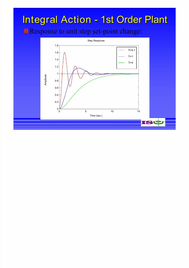
Integral ActionIntegral Action -- 1st Order Plant1st Order Plant

Time (sec.)

A m p l i t u d e

Step Response

0 5 10 150

0.2

0.4

0.6

0.8

1

1.2

1.4

1.6

1.8

Ti=0.1

Ti=1

Ti=4


8/10/2019 L03 ACT PID


Derivative ActionDerivative Action

Objective: stabilise system; slow down transients

PD controller:

In Laplace domain:

With constant error, derivative action = 0 no contribution to steady-state behaviour

With transients on error, derivative action = large

risk actuator saturation from measurement noise, step changes

in set-point

⎟ ⎠

⎞⎜⎝

⎛ +=

dt

deT t e K t u d cc )()(

( ) sT K s K d c += 1)(

8/10/2019 L03 ACT PID


DerivativeDerivative -- on Loop Outputon Loop Output

Derivative often used in feedback path only i.e PI-D control

( ))()()( s syT se K su d cc −=

Plant

G(s)

K C T d s

K C

+

-

+

-

P-D Controller

r(s) y(s)e(s) uC (s)

( ))()()( s syT se K su d cc −=

Eliminating e(s), using e(s) = r(s) - y(s), gives …..

8/10/2019 L03 ACT PID


( ))()()( s syT se K su d cc −=

Plant

G(s)

K C (1+T d s)

K C

+

-

P-D Controller

r(s) y(s)uC (s)

( ))()()()( s syT s y K sr K su d ccc +−=

DerivativeDerivative -- on Loop Outputon Loop Output

Derivative often used in feedback path only i.e PI-D control

K(s)

K ff (s)

( ) sT GK

GK CLTF

d c

c

++

=11

8/10/2019 L03 ACT PID


DerivativeDerivative -- 1st Order Plant1st Order Plant

Plant: Controller:

Closed-loop TF:

Closed-loop pole: as T d is increased, CL response gets slower

Steady state error not effected by T d :

( ) sT K s K

K s K

d c

c ff

+=

=

1)(

)(

( ) cd c

c

K a sT K

K

sr

s y

+++=

1)(

)(

)1()( d cc T K K a s ++−=

( )a

K sT K

a s

se

cd c

ss

+=

++

+→=

1

1

11

1

1

0lim

a s sG

+=

1)(

8/10/2019 L03 ACT PID


DerivativeDerivative -- 1st Order Plant1st Order Plant

Time (sec.)

A m p l i t u d e

Step Response

0 2 4 6 8 100

0.1

0.2

0.3

0.4

0.5

0.6

0.7

Td=1

Td=2

Td=5


8/10/2019 L03 ACT PID


DerivativeDerivative -- 2nd Order Plant2nd Order PlantGeneralised Plant:

Closed-loop TF:

CL natural frequency:

CL damping ratio:

Steady-state error is not effected by T d

22

2

2)(

npnp p

np

s s sG

ω ω ζ

ω

++=

( ) ( ) 222

2

12)(

)(

npcd npcnp p

npc

K sT K s

K

sr

s y

ω ω ω ζ

ω

++++=

d

c

npc

c

pcl T

K

K

K ++

+=

121

ω ζ ζ

cnpncl K += 1ω ω

8/10/2019 L03 ACT PID


DerivativeDerivative -- 2nd Order Plant2nd Order Plant

Time (sec.)

A m p l i t u d e

Step Response

0 0.5 1 1.5 2 2.5 3 3.5 40

0.1

0.2

0.3

0.4

0.5

0.6

0.7

Td=0.1

Td=0.3

Td=0.6


8/10/2019 L03 ACT PID


DerivativeDerivative -- as Rate Feedbackas Rate Feedback

Implementation using direct measure of derivative

Similar to P-D control

with K r = K cT d

G*

K r

K C

+

-

+

-

Controller Plant, G(s)

ω θr(s) y(s)e(s) 1

s

( ) s K K G

GK CLTF

r c

c

++=

1

angular

velocity

angle

8/10/2019 L03 ACT PID


Tuning PID ControllersTuning PID ControllersFundamental Trade-offs

Applicability of PID

Process Reaction Tuning

Sustained Oscillation Tuning

IMC PID Tuning

Advanced Tuning Methods

8/10/2019 L03 ACT PID


Fundamental TradeFundamental Trade--offsoffs

Set-point tracking:

Good tracking performance K(s)G(s) large

Stability:

Keep K(s)G(s) away from -1 limit on K(s)

Disturbance rejection:

Reduce effect of disturbances K(s) large

Noise immunity:

Noise should not excite u(s) limit on K(s)

8/10/2019 L03 ACT PID


PI controllers adequate for most applications

Derivative action is rarely utilised

often misunderstood due to the many different forms and the

different ways in which they work

For dominant second (and higher) order plants

PID control may be more appropriate

additional D term can provide damping to reduce overshoot

D can be beneficial for slow thermal processes

Applicability of PID Applicability of PID

8/10/2019 L03 ACT PID


The following generalisation is from Shinsky

("Process Control Systems", McGraw Hill, 1979)

There will always be exceptions, so need tuning rules ...

Process Proportional Band (%) Integral Derivative

Flow 100-500 essential no

Pressure, liquid 50-200 essential no

Pressure, gas 0-5 no no

Level 5-80 seldom no

Vapour (T and p) 10-100 yes essential

Chemical Composition 100-1000 essential if possible

Applicability of PID Applicability of PID

8/10/2019 L03 ACT PID


Plant in open loop with and input unom

Apply a step to input (u step

) and record the

response

Determine L and R from the response

Process Reaction TuningProcess Reaction Tuning

T

y y

T

y R

nom step

Δ

−=

Δ

Δ=

8/10/2019 L03 ACT PID


Normalise R:

Use L and R N in this table to give PID settings

Process Reaction TuningProcess Reaction Tuning

nom step N

uu

R R

−=

Controller K p T i Td

P 1.0/(R NL) - -

P+I 0.9/(R NL) 3L -

P+I+D 1.2/(R NL) 2L 1/(2L)

8/10/2019 L03 ACT PID


Carried out with plant in closed-loop

useful for open-loop unstable plant

Using a proportional-only controller, increase the

gain until sustained oscillations are attained

need to be careful that oscillations do not upset normal running

Record the gain ( K c) and the period of theobserved oscillations (T c)

Sustained Oscillation TuningSustained Oscillation Tuning

8/10/2019 L03 ACT PID


Use K c and T c in this table to give PID settings

These are just initial values to get the controller

to work

will need “fine tuning”

Sustained Oscillation TuningSustained Oscillation Tuning

Controller K p Ti Td

P 0.5K c - -

P+I 0.45K c 0.8Tc -

P+I+D 0.6K c 0.5Tc 0.125Tc

8/10/2019 L03 ACT PID


“IMC” = Internal Model Control

Requires plant model

model structure and order (e.g. first order with dead-time)

parameters such as gains, dead-time and time constants

usually obtained from plant tests

… and desired closed loop time constant ( β )

IMC formulae give required PID gains for

specified plant model and β

IMC PID TuningIMC PID Tuning

8/10/2019 L03 ACT PID


If the plant model is:

first order - controller = PI

second order - controller = PID

first order + dead-time - controller = PID

For higher order plant models, resulting PID isonly an approximation of true IMC controller

Tools are available that contain the formulae e.g. “EZYtune” (http://www.unac.com.au/ezytune)

IMC PID TuningIMC PID Tuning

8/10/2019 L03 ACT PID


Aström and Hagglund (“Relay”) Auto-tuning:

similar to sustained oscillation method, but uses a relay with

dead-zone to establish oscillations

tuning rules built into controller so that it can perform this test

and automatically re-tune itself

PID tuning using system identification and

closed loop pole placement

called “self-tuning” if carried out on-line and automatically

Advanced Tuning Methods Advanced Tuning Methods

8/10/2019 L03 ACT PID


define desired performance

rise time, peak overshoot, stability margins, etc.

identify the dominant plant dynamics

look at interaction with neighbouring loops

which PID configuration is being used ? consider saturation

examine set-point tracking and disturbance

rejection of CL system

has the desired performance been met ?

Loop Tuning Check ListLoop Tuning Check List

8/10/2019 L03 ACT PID


PID and LeadPID and Lead--Lag ControllerLag ControllerCharacteristicsCharacteristics

PI similar to lag-compensator

PD similar to lead-compensator

…. shown in the following bode plots

PI & L C tPI & L C t

8/10/2019 L03 ACT PID


PI & Lag Compensator PI & Lag Compensator

Frequency (rad/sec)

P h a s e ( d e g ) ; M a g n i t u d e ( d B )

Bode Diagrams

10-2

10-1

100

101

-100

-50

00

20

40

60

PIlag

Bode plot:

Magnitude:

PI: rising for decreasing frequencyLag: levels out at low frequencies

Phase:PI: 90° phase lag for frequencies below breakpoint

Lag: phase lag only between breakpoints

PD & L d C t

8/10/2019 L03 ACT PID


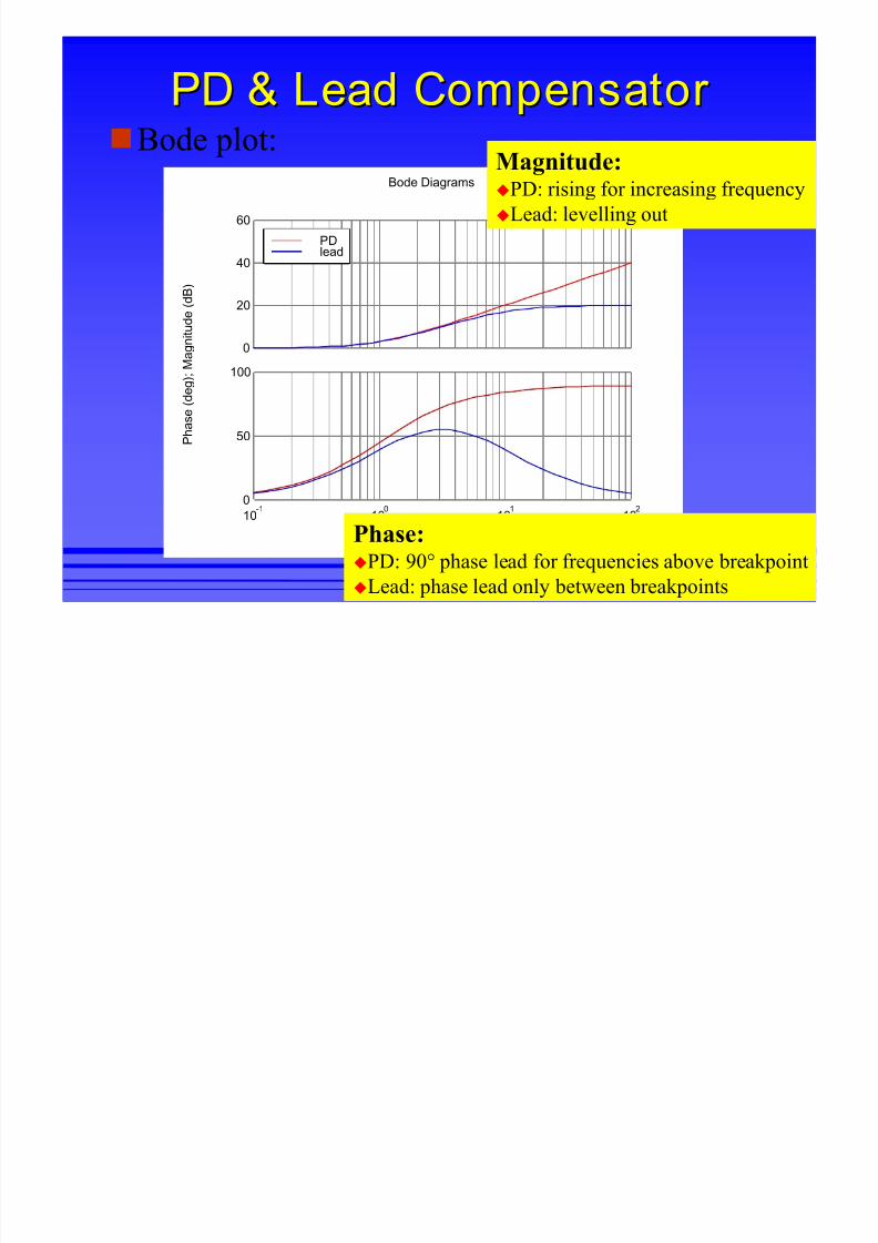
PD & Lead Compensator PD & Lead Compensator

Frequency (rad/sec)

P h a s e ( d e g ) ; M a g

n i t u d e ( d B )

Bode Diagrams

10-1

100

101

102

0

50

100

0

20

40

60

PDlead

Bode plot:Magnitude:PD: rising for increasing frequency

Lead: levelling out

Phase:PD: 90° phase lead for frequencies above breakpoint

Lead: phase lead only between breakpoints

8/10/2019 L03 ACT PID


Implementation Aspects of PIDImplementation Aspects of PID

Bumpless Transfer

Derivative Filtering

Integral Windup

Digital Implementation

8/10/2019 L03 ACT PID


Bumpless Transfer Bumpless Transfer Prevents spiky demand signals to actuators when

switching between different control modes

Occurs when switching from manual to automatic

Cause: controller output different from current signal

Solution: set reference to follow current plant output value

called a “tracking” controller

Derivative action on PV also helps

8/10/2019 L03 ACT PID


Derivative FilteringDerivative FilteringMost industrial PID controllers have some filtering

on derivative actionPrevents noisy measurements giving noisy

controller outputs

Usually applied as:

α = derivative time multiplier

typically in range 0.06 0.13

1+ sT

sT

d

d

α

Integral WindupIntegral Windup

8/10/2019 L03 ACT PID


Integral WindupIntegral Windup

Caused by integral action and actuator saturation

Can lead to instability

Graphical RepresentationGraphical Representation

8/10/2019 L03 ACT PID


Graphical RepresentationGraphical Representation

This “extra control” is a time delay

- which can destabilise the plant.

AntiAnti Windup MechanismsWindup Mechanisms

8/10/2019 L03 ACT PID


Anti Anti --Windup MechanismsWindup Mechanisms

+

Analogue implementation:

In practice it is difficult to set-up gain K

AntiAnti Windup MechanismsWindup Mechanisms

8/10/2019 L03 ACT PID


Anti Anti --Windup MechanismsWindup Mechanisms

Logic/digital implementation easier:

Anti-windup present in most industrial controllers

*

*

Δu1 if Δu = 0

0 if Δu<>0

Di it l I l t ti

8/10/2019 L03 ACT PID


Digital ImplementationDigital Implementation

A continuous time PID controller is given by:

This can be cast into this discrete time form:

where k is the sample number and τ s is the

sampling period

dt

de K dt t e K t e K t u d

t

i pc

∫ ++=0

)()()(

[ ])1()()()()(

0

−−++= ∑=

k ek e K

je K k e K k u s

d k

j

si pcτ

τ

Di it l I l t ti

8/10/2019 L03 ACT PID


Digital ImplementationDigital Implementation

This may be re-written as:

or:

The change in controller output (Δuc) is calculated

and the inherent digital integrator forms uc(k)

Called an “incremental PID” controller

[ ] [ ])2()1(2)()()1()()1()( −+−−++−−+−= k ek ek e K

k e K k ek e K k uk u s

d si pccτ

τ

)()1()( k uk uk u ccc Δ+−=

8/10/2019 L03 ACT PID


8/10/2019 L03 ACT PID


Extra SlidesExtra Slides

Generic EquationsGeneric Equations

8/10/2019 L03 ACT PID


Generic EquationsGeneric Equations

Closed-loop TF from reference to error

Type 0 servo, unit-step steady-state error

Type 1 servo, unit-ramp steady-state error

)(G(s)K(s)1

1)( sr se+=

p ss

k s s K sG s

se

+=⎟⎟

⎠ ⎞

⎜⎜⎝ ⎛

+→=

1

11

)()(1

1

0lim

v ss

k s s K sG s

se

11

)()(1

1

0lim

2 =⎟⎟

⎠

⎞⎜⎜⎝

⎛

+→=

ProportionalProportional -- 2nd Order Plant2nd Order Plant

8/10/2019 L03 ACT PID


ProportionalProportional 2nd Order Plant2nd Order Plant

SteadySteady--State Error State Error

If K c larger, error smaller

c

nn

cn

ss

K s s

K s s K sG s

s

s

e

+

=

+++→

=

+→

=

1

1

21

1

0

lim

)()(1

11

0

lim

22

2

ω ζω ω

8/10/2019 L03 ACT PID


Integral control:

Proportional-integral control:

01

0

0

110lim

111

1

0lim =

+=

++→

=

++→

=

iii

ss

aT T a s s

s

s

sT a s

se

011

0110

lim1

11

1

10

lim ==

⎟⎟ ⎠

⎞⎜⎜⎝

⎛ +

++

→=

⎟⎟ ⎠

⎞⎜⎜⎝

⎛ +

++

→=

ic

ic

ic

ss

T K

aT s K

a s s

s s

sT K

a s

se

⎟⎟ ⎠

⎞⎜⎜⎝

⎛ +=

sT K s K

ic

11)(

Integral ActionIntegral Action -- 1st1st--Order PlantOrder PlantSteady State Error Steady State Error

DerivativeDerivative - 2nd Order Plant2nd Order Plant

8/10/2019 L03 ACT PID


DerivativeDerivative -- 2nd Order Plant2nd Order Plant

Steady-state error:

( )

c

d cnpnp p

np

d c

npnp p

np

ss K

sT K s s

sT K s s

se

+=

++++

+++

→=

1

1

121

21

0lim

22

2

22

2

ω ω ζ

ω

ω ω ζ

ω

l03 act pid

Documents