Wave Optics Analysis of Coherent Optical p y pSystemsAppendix B Introduction to Paraxial Geometrical Opticspp pB.1 The Domain of Geometrical OpticsB.2 Refraction, Snell’s Law, and the Paraxial ApproximationB.3 The Ray Transfer MatrixB.4 Conjugate Planes, Focal Planes, and Principal PlanesB 4 Conjugate Planes Focal Planes and Principal PlanesB.4 Conjugate Planes, Focal Planes, and Principal Planes5.1 A thin lens as a Phase Transformation

5.1.1 The thickness function5.1.2 The paraxial approximation5.1.3 The Phase Transformation and its Physical Meaning

5.2 Fourier Transforming Properties of Lenses5.2.1 Input placed against the Lens5.2.2 Input Placed in Front of the Lens5.2.3 Input Placed Behind the Lens5 2 4 Example of an Optical Fourier Transform5.2.4 Example of an Optical Fourier Transform

5.3 Image Formation: Monochromatic Illumination5.3.1 The impulse Response of a Positive Lens5.3.2 Eliminating Quadratic Phase Factors: The Lens Law5.3.3 The Relation Between Object and Image

5 4 A l i f C l C h t O ti l S t

1

5.4 Analysis of Complex Coherent Optical Systems5.4.1 An operator Notation5.4.2 Application of the Operator Approach to Some Optical Systems

Goal: understand the relationship of the geometrical optics and physical optics

B.1 The Domain of Geometrical OpticsGoal: understand the relationship of the geometrical optics and physical optics

Subject of interest is the physical optics formulation of the imaging and spatial

filtering and the related concepts in geometrical optics.

Wavelength of the light is always the same but

if the variations or changes of the amplitude and phase of a wavefield take

place on spatial scales that are much larger than the wavelengthplace on spatial scales that are much larger than the wavelength, then predictions of the geometrical optics become accurate.Things that take us out of the relm of the geometrical optics:

A h d A sharp edge A sharply defined aperture A sharp change of the phase by a significant fraction of 2 over a spatial π

~

scales comparable to 1Example: a grating with has to be treted by physical optics N

λ

λ

2

1 a grating can be treateN

λ>> d by geometrical optics

The Concept of a RayA ray traces the path of power flow in an isotropic mediumA ray traces the path of power flow in an isotropic medium.

What does this mean?A monochromatic disturbance traveling in a medium with an index gof refraction that varies slowly compared to the wavelength of the disturbance is expressd by:

( ) ( ) ( )

( )

00

0

2Phase

0

Amplitude

where and is the free space wavelength.jk S rU r A r e k π λλ

= =

( ) or the contains the effect of the refractive index.S r Eikonal Function

Wavefro ( ) are surfaces defined by constantnts S r =

In an isotropic medium: direction of the power flow and

direction of the wavevector are both normal to thek wavefronts

3

.

.

direction of the wavevector are both normal to the

at each point

k wavefronts

r

The geometrical optics limit & Eikonal Equation( ) ( ) ( ) ( ) ( )0 2 02 must satisfy the Helmholtz equation jk S rU r A r e k U r= ∇ + =( )

( ) ( ) ( )( ) ( ) ( )( ) ( ) ( )( ) ( )

( ) ( ) ( ) ( ) ( )( ) ( ) ( )( ) ( )( )0 0 0

0 0

0

20

1)

2)

jk S r jk S r jk S r

jk S r jk S r

U r A r e A r e A r jk S r e

U r U r A r e A r jk S r e

∇ =∇ = ∇ + ∇

∇ = ∇ ∇ = ∇ ∇ + ∇i i ( ) ( )( )( ) ( ) ( ) ( )( ) ( ) ( )( ) ( )0 02 2

02 jk S r jk S rk U r A r e A r jk S r e∇ + = ∇ +∇ ∇ +i ( ) ( )( ) ( )

( ) ( )( ) ( ) ( ) ( )( ) ( ) ( ) ( )

0

0 0 0

0

22 2 20 0 0 0

jk S r

jk S r jk S r jk S r

A r jk S r e

A r jk S r e A r jk S r e n k A r e

∇ ∇

+ ∇ + ∇ + =

i

( ) ( )( ) ( ) ( )( ) ( )

( ) ( ) ( ) ( ) ( ) ( ) ( )0 0 0

22 2 2 20 0 2 0

We require the both real and imaginary parts be equal to zero independ

j j

A r k n S r A r jk A r S r A r S r⎡ ⎤ ⎡ ⎤∇ + − ∇ + ∇ ∇ + ∇ =⎣ ⎦⎢ ⎥⎣ ⎦i

etly.

( ) ( ) ( ) ( ) ( )

( )

22 22 2 2 2 0

0

2 2

02

A h ll d

A rA r k n S r A r S r n

Aλπ

∇⎛ ⎞⎡ ⎤∇ + − ∇ = → ∇ = + ⎜ ⎟⎢ ⎥⎣ ⎦ ⎝ ⎠

( ) 2 20 0As we get the so called

perhaps is the most important equation on the behavior of light under

Eikonal equation S r n

Eikonal equation

λ → ∇ =

. the geometrical optics approximation

4

g p pp

The defines the and therfore the trajectory of the . means image in Greek.

Eikonal equation wavefront raysEikon

B.2 Refraction, Snell’s Law, and the Paraxial ApproximationParaxial Approximation

( ) ( )2 2

)

It can be derived from the Eikonal equation that rays in a

a) homogeneous medium (constant always travel in straight lines

S r n r

n

∇ =

))

a) homogeneous medium (constant always travel in straight lines.b) inhomogeneous medium (varying have curved trajectories th

nn at depend

on the changes of index of refraction.

1 1 2 2

'sin sin

Waves encountering abrupt changes of experience abrupt changes in direction of propagation. This is formulated in :

nSnell s law

n nθ θ=1 1 2 2sin sinApplying n nθ θ

1 1 2 2

sin cos 1'

the where and the becomes

paraxial approximationSnell s law n n

θ θ θθ θ

≈ ≈=

1 2

'Defining the we have a simple form for reduced angle n Snell s lawθ θ

θ θ

=

=

5

B.3 The Ray Transfer MatrixAn equivalent formalism to the operator methods of the physical optics in geometrical

optics is the matrix formalism which is valid under paraxial approximation.To apply the matrix formalism we need to limit ourselves to rays.meridonalMeridonal rays are the rays that are traveling in a single plane containing the axis.The transevers axis in the plane is caled axis by tradition.In figu

zmeridonal y

re a typical ray propagation problem is demonstrated.

2 2

1 1

Goal: to determine the position and angle of the output in termsof the position and angle of the input.Fact: under the paraxial approxi

yy

θθ

mation theA t i l ti bl

( ) ( )2 2 1 1

2 1

, ,relationship between and are linear and written as:

y y

y yy Ay B A B

θ θ

θ⎧ ⎛ ⎞ ⎛ ⎞= + ⎛ ⎞⎪ θθ2

y1 y

A typical ray propagation problem

Input

Output ray

2 12 1 1

2 12 1 1

the matrix is called

y yy Ay B A BC DCy D

A BC D

θθ θθ θ

⎧ ⎛ ⎞ ⎛ ⎞= + ⎛ ⎞⎪ → =⎜ ⎟ ⎜ ⎟⎨ ⎜ ⎟= + ⎝ ⎠⎪ ⎝ ⎠ ⎝ ⎠⎩

⎛ ⎞= ⎜ ⎟⎝ ⎠

M

Optical system z

z1I t

z2Output

θ1y1 y2

Input ray

6

- matrix or the C D

ray transfer ABCD

⎜ ⎟⎝ ⎠

matrix.Input plane

Outputplane

2.2 Spatial frequency and space-frequency localization IEach Fourier component of a function is a complex exponential function of a unique spatial frequency. Therefore every frequency component

( , )

q p q y y q y p

extends over the entire domain.

So we can't associate a

x y

spatial location for a particular spatial frequency.

( )

( )

2 ( )

2 ( )

( , ) ,

( , ) ,

X Y

X Y

j f x f yX Y X Y

j f x f yX Y

g x y G f f e df df

G f f g x y e dxdy

π

π

∞ +

−∞

∞ − +

=

=

∫ ∫∫ ∫ ( )( , ) ,

In practice certain portions of an image could contain parallel grid linesX Yf f g y y

−∞∫ ∫at

a certain fixed spaing. We tend to say these frequencies are localized to the certain spatial regions of the image.

What is the relationship of the local spatial frequencies or ( and ) with lX lYf fthe spatial frequencies of the Fourier components?

7

the spatial frequencies of the Fourier components?

Spatial frequency and space-frequency localization II

( , )( , ) ( , ) ( , )( , )

Consider a complex valued function: where is a positive slowly varying amplitude function and is a real phase distribution.

j x yg x y a x y e a x yx y

φ

φ=

We define the local spatial frequency ( , )( , ) ( , ) :1 1( , ) ( , ) 0 0 ( , ) 0

2 2

of the function

and also & if

j x y

lX lY lX lY

g x y a x y e

f x y f x y f f g x yx y

φ

φ φπ π

=∂ ∂

= = = = =∂ ∂

When the rate of phase change is constant we have a fixed as rate chages then

we move tlf

2 ( )( , ) ( , ) 11 1( ) ( )

o a different . Now for with we obtain

d

X Yj f x f ylf g x y e a x y

f f f f f f f f

π += =

∂ ∂1 12 ( ) 2 ( )2 2

and

So for the case of a single Fourier component the local spatial frequencies

lX X Y X lY X Y Yf f x f y f f f x f y fx y

π ππ π

∂ ∂= + = = + =

∂ ∂

( )and are the same and span over the entire plane (no localization)f f x y( ), and are the same and span over the entire plane (no localization).lf f x y

8

Spatial frequency and space-frequency localization IIINow we consider a space limited version of the quadratic phase

2 2( ) ) :

exponent or a finite chirp function (chirp function is another name for

the infinite-length quadratic phase exponent j x ye πβ +

⎛ ⎞ ⎛ ⎞( , )g x y =

2 2( )

2 2

2 2

1 ( )

j x y

X Y

x ye rect rectL L

x xf

πβ

β β

+ ⎛ ⎞ ⎛ ⎞⎜ ⎟ ⎜ ⎟⎝ ⎠ ⎝ ⎠

⎛ ⎞ ⎛ ⎞∂⎜ ⎟ ⎜ ⎟

2 2

2 2

1 ( )2 2 2

1 ( )

lXX X

lY

x xf rect x y x rectL x L

y yf rect x y y rect

πβ βπ

πβ β

⎛ ⎞ ⎛ ⎞∂= + =⎜ ⎟ ⎜ ⎟∂⎝ ⎠ ⎝ ⎠

⎛ ⎞ ⎛ ⎞∂= + =⎜ ⎟ ⎜ ⎟( )

2 2 2

2 2We see now that and

lYY Y

lX lYX

f y yL y L

x yf x rect f y rectL

β βπ

β β

⎜ ⎟ ⎜ ⎟∂⎝ ⎠ ⎝ ⎠⎛ ⎞

= =⎜ ⎟⎝ ⎠

both YL

⎛ ⎞⎜ ⎟⎝ ⎠X⎝ ⎠

( )1

,2 2 .depend on location on the plane within the rectangle of dimensions

, varies linearly with and varies linearly with

Y

X Y lX Y

x yL L f x f y

⎝ ⎠

×

9

So for this function and many other functions t

( ),

here is a dependence of

local spatial frequenciy on the position in the plane.x y

Local Spatial Frequencies and the Ray-Transfer MatrixRay Transfer Matrix

-Relationship of the local spatial frequencies and the matrix:

Under the paraxial approximation the reduced ray angle is related to lf ray transfer

θp pp y g the local spatial frequencies throughl

l

f

f θ θλ λ

= =0

W

lf λ λe see that local spatial frequencies of a coherent optical wavefront

correspond to the ray directions of the geometrical optics description

2 1 2

of that wavefront.y y yA B⎛ ⎞ ⎛ ⎞ ⎛⎛ ⎞

= →⎜ ⎟ ⎜ ⎟⎜ ⎟1yA B⎞ ⎛ ⎞⎛ ⎞

=⎜ ⎟ ⎜ ⎟⎜ ⎟2 02 1 lfC D λθ θ

⎜ ⎟ ⎜ ⎟⎜ ⎟⎝ ⎠⎝ ⎠ ⎝ ⎠ 1 0

,So the ray-transfer matrix relates the spatial distribution of the local spatial frequencies (or ray directions) at the output to the spatial

l

l

fC D

f

λ⎜ ⎟ ⎜ ⎟⎜ ⎟⎝ ⎠⎝ ⎠ ⎝ ⎠

M

10

oca spat a eque c es (o ay d ect o s) at t e output to t e spat adistribution of the

l

l

ff (or ray direction) at the input.

Elementary Ray-Transfer Matrices IR f i f i

.Ray-transfer matix of some important structures1. Propagation through free space of index

The angle of propagation stays unchnged

n

θ θ θ2 1

2 12 tan

The angle of propagation stays unchnged

while changes y yyd

θ θ θ

θ θ

= =−

≈ =

2 1

2 1

y yA BC Dθ θ

⎛ ⎞ ⎛⎛ ⎞=⎜ ⎟ ⎜ ⎟⎝ ⎠⎝ ⎠

1 1d y yA BC D

θ

θ θ

+⎞ ⎛ ⎞ ⎛ ⎞⎛ ⎞→ =⎜ ⎟ ⎜ ⎟ ⎜ ⎟⎜ ⎟

⎝ ⎠⎝ ⎠ ⎝ ⎠⎝ ⎠A t i l ti bl

1 1

1

d y Ay B

Cy D

θ θ

θ θ

⎧ + = +⎪→ ⎨+ =⎪⎩

θ

θ2

y1 y

A typical ray propagation problem

Input d

1 /

Therefore a matrix that satisfies the above equation has the form:

d⎛ ⎞

Optical system z

z1I t

z2Output

θ1y1 y2

Input ray

d

11

1 /0 1

d n⎛ ⎞= ⎜ ⎟⎝ ⎠

MInput plane

Outputplane

n n n

Elementary Ray-Transfer Matrices II

2 1 2 1 1

.2. Refrction at a planar interface

y y y Ay BA B θ⎧⎛ ⎞ ⎛ ⎞ = +⎛ ⎞ ⎪= →⎜ ⎟ ⎜ ⎟ ⎨⎜ ⎟2 1 2 1 1

2 1

2 2 1 1

At a planar interfac the angle of propagation change but according to the Snell's law

C D Cy D

n n

θ θ θ θθ θ

θ θ

⎜ ⎟ ⎜ ⎟ ⎨⎜ ⎟= +⎝ ⎠ ⎪⎝ ⎠ ⎝ ⎠ ⎩

≠=2 2 1 1according to the Snell s law n nθ θ

2 1

2 1

Therefore the reduced angle remains unchanged while position of the ray is unchanged y y

θ θ==

Therefore a matrix that satisfies the above equation has the form: θ θInput

1 00 1

the above equation has the form:⎛ ⎞

= ⎜ ⎟⎝ ⎠

M zz2Output

θ1 θ2y1

y2

Input ray

12

Outputplane

n1n2

Optical system

Elementary Ray-Transfer Matrices III3 R f ti t h i l i t f

1 2

2

.3. Refrction at a spherical interface At a spherical interfac the position of ray is not changed while the angle of propagation with respect the the normal to the surface, change according

y y y

φ

= =

2 2 1 1to the Snell's law n nφ φ=

θ1θ2

y1y2

Input ray

2surface, change accordingφ 2 2 1 1

1 1 1 1 2 2arcsin

to the Snell s law The relationship of the to the angle with the optical axis is

where so and

n n

y y y yR R R R

φ φφ θ

φ θ ψ ψ φ θ φ θ= + = ≈ = + = +

z

2 2 1 1 1 1 1 2 2 2 1 1 2With y y yn n n n n n nR R R

φ φ θ θ θ θ= → + = + → + =

( )2

1 22 1

ynR

n ny

Rθ θ

+

−= +

n1 n2

θ

( ) ( )1

1 2 1 211 1 1

Therefore a matrix that satisfies

y y Ay ByA Bn n n nC Dy y Cy D

R R

θ

θθ θ θ

⎧ = +⎛ ⎞ ⎛ ⎞⎛ ⎞ ⎪⎜ ⎟ = →⎜ ⎟− ⎨⎜ ⎟ −⎜ ⎟+ + = +⎝ ⎠⎜ ⎟ ⎝ ⎠ ⎪⎝ ⎠ ⎩ R

φ1 φ2θ1

θ2y1

( )1 2

1 0

1

Therefore a matrix that satisfies the above equation has the form:

n n⎛ ⎞⎜ ⎟= −⎜ ⎟⎜ ⎟

M

13

( )1

A positive valuR

⎜ ⎟⎜ ⎟⎝ ⎠

e for R satisfies the convex surface encountered from left to right.A negative value for R satisfies the concave surface encountered from left to right.

Elementary Ray-Transfer Matrices IV4 P th h thi l

2 1

1 2

.4. Passage through a thin lens

A thin lens with index embedded in a medium of can be treated by cascading two spherical interfaces. for the second surface roles of

and are switched. Ray-t

n n

n n ransfer matix of the1 2 and are switched. Ray tn n

( ) ( )1 21 2 2 1

1 2

1 0 1 0

1 1

ransfer matix of the

surface 1: and surface 2: n n n nR R

⎛ ⎞ ⎛ ⎞⎜ ⎟ ⎜ ⎟= =− −⎜ ⎟ ⎜ ⎟⎜ ⎟ ⎜ ⎟⎝ ⎠ ⎝ ⎠

M M

( )2 12 1

1 2

1 0

1 1 1The total effect of both syrfaces:

n nR R

⎛ ⎞⎜ ⎟

= = ⎛ ⎞⎜ ⎟− − −⎜ ⎟⎜ ⎟⎝ ⎠⎝ ⎠

M M M

⎛ ⎞

s1 s2 sn

Defining the focal length of the 2 1

1 1 2

1 1 1

1 0

lens: n nf n R R

n

⎛ ⎞−= −⎜ ⎟

⎝ ⎠⎛ ⎞⎜ ⎟= ⎜ ⎟M

R1R2

z1 1

To use the Ray-transfer matrix for many instruments and surfaces, the matrices should appear in the order which the ray has emcountered them.

nf

= ⎜ ⎟−⎜ ⎟⎝ ⎠

M

n2n1 n1

….

nn

14

2...n=M M M M1

Since we have used the reduced angles insted of real angles, determinantof all the transfer matrices have become unity.

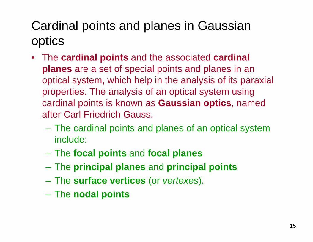
Cardinal points and planes in Gaussian opticsoptics• The cardinal points and the associated cardinal

planes are a set of special points and planes in an optical system, which help in the analysis of its paraxial properties. The analysis of an optical system using cardinal points is known as Gaussian optics, namedcardinal points is known as Gaussian optics, named after Carl Friedrich Gauss.– The cardinal points and planes of an optical system

i l dinclude:– The focal points and focal planes

The principal planes and principal points– The principal planes and principal points– The surface vertices (or vertexes). – The nodal points

15

e oda po ts

B.4 Conjugate PlanesConjugate planes: Two planes or points within an optical system are said to be conjugate j g p p p p y j g

planes if intensity distribution across one plane is an image of the intensity distribution

across the other pla

2 1 1

ne.

U i h f th j t i t th i t d t t ly Ay Bθ⎧ = +⎪

⎨2 1 1

2 1 1

2 1

Using we can show for the conjugate points on the input and output plane

1) the position of the point should be independent of the reduced angle of a ray throug

y y

Cy D

y

θ θ

θ

⎪⎨

= +⎪⎩

1 0. therefore y B =

2 1

2

2) .

3)

where is the transverse magnification. Therefore

the angles of the rays passing through will be maginfied or demagnified with respect to the angles of the

t t ty m y m A m

y

= =

1.rays arriving from If y m reduced angular magnificationα =

( )

2 1

1

.0

0

( / )

then Therefore

And

Angle and position are conjugate Fourier variables

t

m D mm

m

k k

α α

α

θ θ

−

= =

⎛ ⎞= ⎜ ⎟⎝ ⎠

M

( )1cos ( / )Angle and position are conjugate Fourier variables.

The similarity (scaling) thyk k y

-11 1 2 2 1 2 2 1 1

01 / / 1

0

eorem implies that

tt t

my y y y m m m m

mα αθ θ θ θ −

⎛ ⎞= = → = → = → = → = ⎜ ⎟

⎝ ⎠M

16

0

1

Note and can be both positive and negative but they have to be of the same sign.

Nonparaxial form of the

t

t

t

mm m

m mα

α

⎝ ⎠

= 1 1 1 2 2 2sin sinis caled sine condition: n y n yθ θ=

B.4 Focal PlanesFor a parallel bundle of rays traveling parallel to the optical axis and entering a lens, there always o a pa a e bu d e o ays a e g pa a e o e op ca a s a d e e g a e s, e e a ayswill exist a point on the optical axis toward which the ray bundle converge (positive lanse) or f

0

rom which it will appear to diverge (negative lens). If is the focal length of the lens, then the ray-transfer f

f⎛ ⎞⎜ ⎟

1

1

0

0matrix between the focal planes takes the forrm Exercise: p

nnf

⎜ ⎟⎜ ⎟=⎜ ⎟−⎜ ⎟⎝ ⎠

M rove this

Rear focal point

f

Front focal point

ff2Rear focal plane

f1Front focal plane

Front focal point

Rear focal point

f

17

f1Front focal plane

f2Rear focal plane

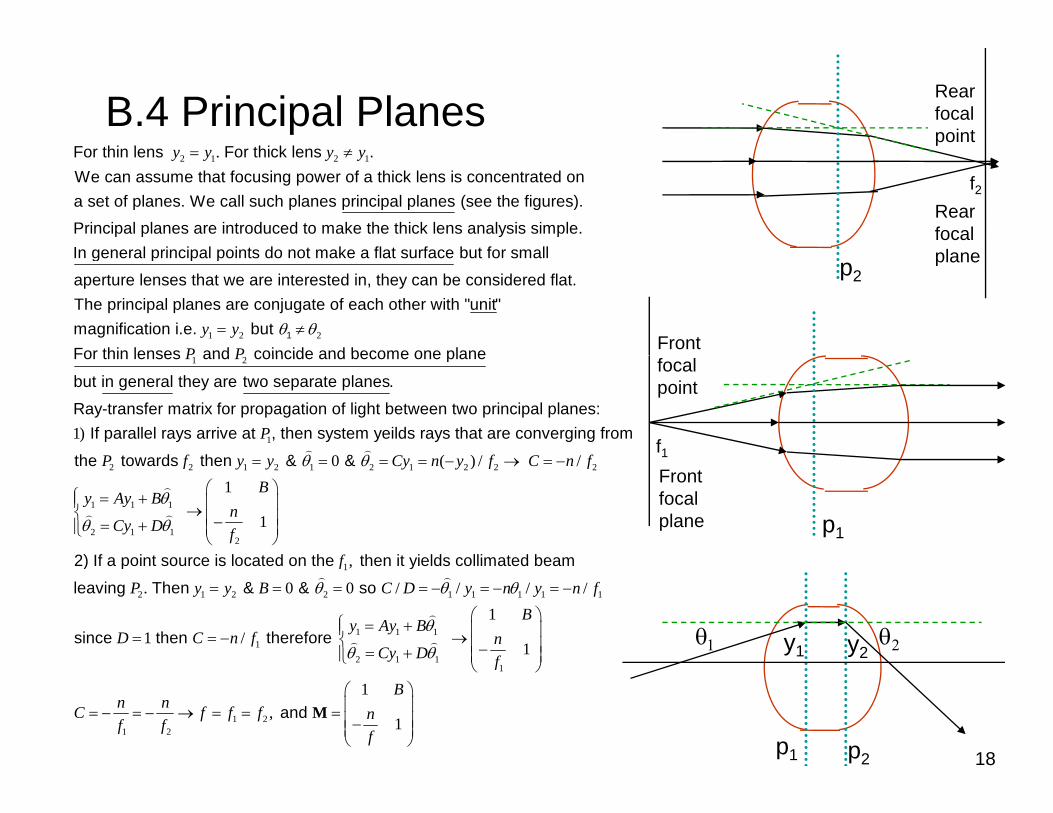
B.4 Principal PlanesFor thin lens For thick lensy y y y≠

Rear focal point

2 1 2 1.For thin lens For thick lens .We can assume that focusing power of a thick lens is concentrated on a set of planes. We call such planes principal planes (see the figures). Principal plane

y y y y= ≠

s are introduced to make the thick lens analysis simple.In general principal points do not make a flat surface but for small

f2Rear focal planeIn general principal points do not make a flat surface but for small

aperture lenses that we are interested in, they can be considered flat.The

1 2 21

principal planes are conjugate of each other with "unit" magnification i.e. but For thin lenses and coincide and become one plane

y yP P

θ θ= ≠Front

planep2

1 2For thin lenses and coincide and become one plane

but in general they are two separate planes.

Ray-trans

P P

11)

0 (

fer matrix for propagation of light between two principal planes: If parallel rays arrive at , then system yeilds rays that are converging from

the towards then & &

P

P f Cθ θ ) / /f C f→

focal point

f12 2 1 2 1 2 10 (the towards then & & P f y y Cy n yθ θ= = = = − 2 2 2

1 1 1

2 1 12

) / /1

1

2) If a point source is located on the then it yields collimated beam

f C n fB

y Ay Bn

Cy D ff

θ

θ θ

→ = −

⎛ ⎞⎧ = +⎪ ⎜ ⎟→⎨ ⎜ ⎟−= +⎪ ⎜ ⎟⎩ ⎝ ⎠p1

Front focal plane

1

2 1 2 2 1 1 1 1 1

,

. 0 0 / / / /

2) If a point source is located on the then it yields collimated beam

leaving Then & & so

f

P y y B C D y n y n fθ θ θ= = = = − = − = −

1 1 11

2 1 1

11 /

1

since then therefore B

y Ay BD C n f n

Cy D f

θ

θ θ

⎛ ⎞⎧ = +⎪ ⎜ ⎟= = − →⎨ ⎜ ⎟−= +⎪ ⎜ ⎟⎩ ⎝ ⎠y1

θ1 θ2y2

18

1

1 21 2

1,

1 and

f

Bn nC f f f nf f

f

⎩ ⎝ ⎠⎛ ⎞⎜ ⎟= − = − → = = = ⎜ ⎟−⎜ ⎟⎝ ⎠

M

p2p1

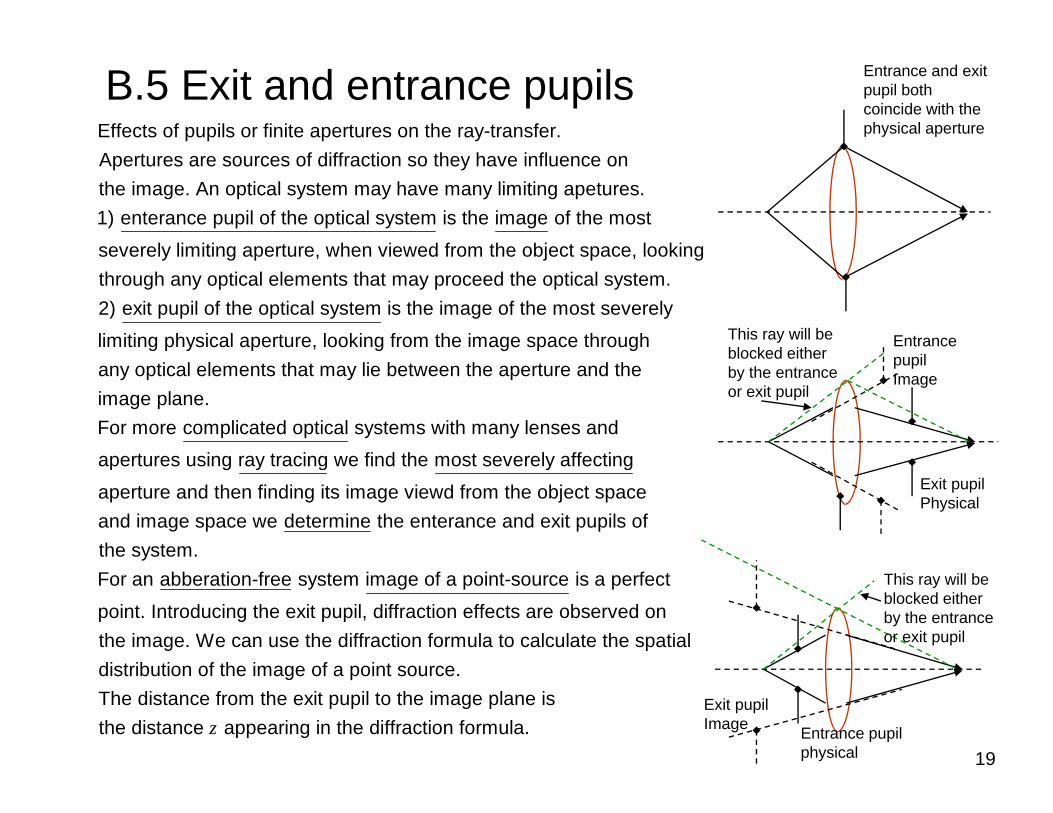
B.5 Exit and entrance pupilsEffects of pupils or finite apertures on the ray-transfer.

Entrance and exit pupil both coincide with the physical aperture

Apertures are sources of diffraction so they have influence on the image. An optical system may have many limiting apetures. 1) enterance pupil of the optical system is the image of the most

severely limiting aperture when viewed from the object space lookingseverely limiting aperture, when viewed from the object space, looking through any optical elements that may proceed the optical system.2) exit pupil of the optical system is the image of the most severely

limiting physical aperture, looking from the image space through Entrance il

This ray will be blocked either

any optical elements that may lie between the aperture and the image plane. For more complicated optical systems with many lenses and apertures using ray tracing we find the most severely affecting

pupilImage

blocked either by the entrance or exit pupil

apertures using ray tracing we find the most severely affecting

aperture and then finding its image viewd from the object space and image space we determine the enterance and exit pupils of the system.

Exit pupilPhysical

yFor an abberation-free system image of a point-source is a perfect

point. Introducing the exit pupil, diffraction effects are observed on the image. We can use the diffraction formula to calculate the spatial di t ib ti f th i f i t

This ray will be blocked either by the entrance or exit pupil

19

distribution of the image of a point source. The distance from the exit pupil to the image plane is the distance appearing in the z diffraction formula. Entrance pupil

physical

Exit pupilImage

The Surface Vertices and Nodal points• The surface vertices are the points where each

surface crosses the optical axis. They are important primarily because they are the physically measurable parameters for thephysically measurable parameters for the position of the optical elements, and so the positions of the other cardinal points must be known with respect to the vertices to describe the physical system.

Front surface vortex

θp y y

• The front and rear nodal points have the property that a ray that passes through one of them will also pass through the other, and with

Optical axis

R

v1

v2N1

N2

θ2

θp gthe same angle with respect to the optical axis. The nodal points therefore do for angles what the principal planes do for transverse distance. If the medium on both sides of the optical system is the same (e g air) then the front and

Rear surface vertex

θ1

system is the same (e.g. air), then the front and rear nodal points coincide with the front and rear principal planes, respectively.

• Exercise: Find the transfer matrix for the nodal points

20

nodal points

5.1 A thin lens as a Phase Transformation1lens: an optically dense material with > Different phase

( )

1

,

lens: an optically dense material with Speed of light is less than in a lens.Thin lens: a ray arriving at coordinates on one face, exits at approximately the same coordinates on the opposite

nc

x y

>

2 1.face or y y=

pdelays causing different k vectors

pp y pp 2 1

A thin lens simply delays an incident wavefront by an amount

proportional to the thickness of the lens at each point. Phase delay means change in the wavefront shape, therefore

y y

n

change in

0

( , ) ,( )

direction of parpagation vector. We define:

Maximum thickness Thickness at coordinates

Total phase delay suffered by the wave at passing throughx y x y

x y

Δ =

Δ = Δ(x,y)

x or ySide view

0

( , )

( , ) ( , ) ( ,

Total phase delay suffered by the wave at passing through

the lens:

x y

x y k k x y kn x yφ = Δ − Δ + Δ )The lens may be represented by a multiplicative

nz

Δ0

[ ]

( ) ( )

0 ( 1) ( , )

' , ,

phase transformation of the form:jk n x yjk

l

l l

t e e

U x y t x y

− ΔΔ=

= ( , )lU x y

yFront view

21

Complex field across Phase delay a plane imediately caused by behind the lens the

( )'

( , ),

Complex field incidenton a plane imediatelyin front of the lens lens

If we know the mathematical form of the thickness function then we can calculate and unederstand the efl

x yU x y

Δ

fects of the lens.

x

5.1.1 The thickness functionΔ02

( , )Goal: define the thickness function for a lens. Sign convention:Rays travel from left to right.1) Radius of convex surfaces encountered

x yΔ y

r1) Radius of convex surfaces encounteredby the lens are positive. 2) Radius of concave surfaces encountered by the lens are negative

R1

(x,y)x

( )

( ) ( ) ( ) ( ) 2 2 2

,

by the lens are negative.

To find we split the lens to three parts and write the total thicknes function as:

with

x y

x y x y x y x y r x y

Δ

Δ = Δ + Δ + Δ = +

2 2 21 1R R x y− − −

( ) ( ) ( ) ( )

( ) ( )1 2 3

2 22 2

1 01 1 1 01 1 21

, , , ,

, 1 1

with x y x y x y x y r x y

x yx y R R r RR

Δ = Δ + Δ + Δ = +

⎛ +Δ = Δ − − − = Δ − − −

⎝( )

⎞⎜ ⎟⎜ ⎟

⎠Δ Δ

Δ01

(x,y)R( )

( ) ( )2 02

2 22 2

3 03 2 2 03 2 22

,

, 1 1

x y

x yx y R R r RR

Δ = Δ

⎛ ⎞+Δ = Δ − − − − = Δ + − −⎜ ⎟⎜ ⎟

⎝ ⎠ 2 2 22 2R R x y− − − −

R2

22

( )2 2 2 2

0 1 22 21 2

0 01 02 03

, 1 1 1 1

Where

x y x yx y R RR R

⎛ ⎞ ⎛ ⎞+ +Δ = Δ − − − + − −⎜ ⎟ ⎜ ⎟⎜ ⎟ ⎜ ⎟

⎝ ⎠ ⎝ ⎠Δ = Δ + Δ + Δ

2 2R R x y

Δ03

5.1.2 The paraxial approximationGoal: to simplify the thickness function for the cases that are restricted to portions of wave near the lens axis. That means al es of and are s fficientl small to rite

2 2 2 2

2 21 12

That means values of and are sufficiently small to write:

a

x y

x y x yR R+ +

− ≈ −2 2 2 2

2 21 12

nd x y x yR R+ +

− ≈ −1 12R R 2 2

2 2 2 2

2Then we have:

R R

⎛ ⎞ ⎛ ⎞( )

2 2 2 2

0 1 22 21 2

2 2 2 2

, 1 1 1 1x y x yx y R RR R

⎛ ⎞ ⎛ ⎞+ −Δ = Δ − − − − − −⎜ ⎟ ⎜ ⎟⎜ ⎟ ⎜ ⎟

⎝ ⎠ ⎝ ⎠⎛ ⎞ ⎛ ⎞⎛ ⎞ ⎛ ⎞( )

2 2 2 2

0 1 22 21 2

2 2

, 1 1 1 12 2

1 1

x y x yx y R RR R

⎛ ⎞ ⎛ ⎞⎛ ⎞ ⎛ ⎞+ +Δ ≈ Δ − − − − − −⎜ ⎟ ⎜ ⎟⎜ ⎟ ⎜ ⎟⎜ ⎟ ⎜ ⎟⎝ ⎠ ⎝ ⎠⎝ ⎠ ⎝ ⎠

⎛ ⎞

23

( )2 2

01 2

1 1,2

x yx yR R

⎛ ⎞+Δ ≈ Δ − −⎜ ⎟

⎝ ⎠

5.1.3 The Phase Transformation and its physical meaningphysical meaning

( ) [ ]

( ) ( )

0 ( 1) ( , )

'

,

( )

The lens representation as a multiplicative phase transformation:jk n x yjk

lt x y e e

U U

− ΔΔ=

( ) ( )

( ) ( )2 2

01 2

, , ( , )

1 1, ,2

Substituting in we get:

l l l

l

U x y t x y U x y

x yx y t x yR R

=

⎛ ⎞+Δ ≈ Δ − −⎜ ⎟

⎝ ⎠

( )2 2

010

1 1( 1)2,

x yjk nRjk

lt x y e e+

− Δ − −Δ=

2 2

2 1 20

1 1( 1)2

We combine physical properties of the lens in a single parameter

x yjk nR R Rjkne e

f

⎡ ⎤⎛ ⎞⎛ ⎞ ⎡ ⎤⎛ ⎞+⎢ ⎥⎜ ⎟ − − −⎜ ⎟ ⎢ ⎥⎜ ⎟⎜ ⎟⎢ ⎥ Δ ⎢ ⎥⎝ ⎠⎝ ⎠ ⎝ ⎠⎣ ⎦ ⎣ ⎦=

( )( )2 2

0 2

1 2

1 1 1( 1) , .

p y p p g p

then

f

kj x yfjkn

l

f

n t x y e ef R R

⎡ ⎤− +⎢ ⎥Δ ⎣ ⎦⎛ ⎞

= − − =⎜ ⎟⎝ ⎠

f fIf we neglect the constant phase factor, the basic representation of the effects of a thin lens on the incident distribution as a pahse transformation factor can be written as:

24

( )( )2 2

2,We have no

kj x yf

lt x y e⎡ ⎤− +⎢ ⎥⎣ ⎦=

t acounted for the finite extent of the lens here.

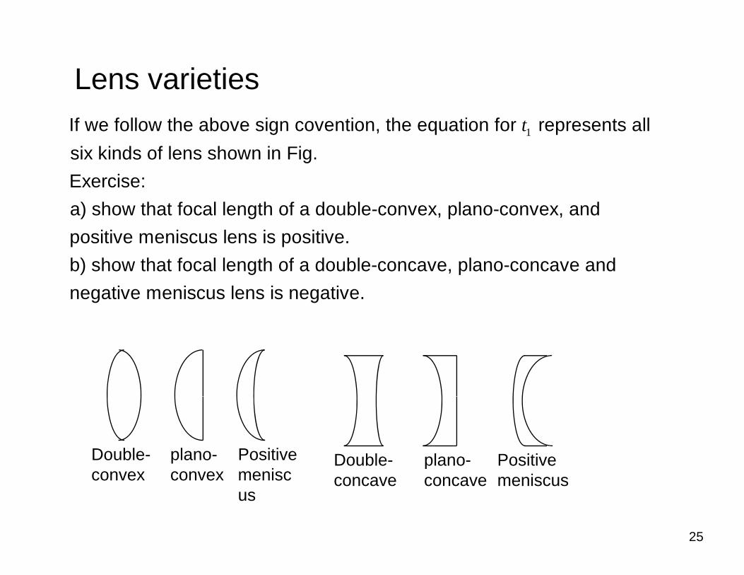
Lens varieties1If we follow the above sign covention, the equation for represents all

six kinds of lens shown in Fig.Exercise:

t

Exercise: a) show that focal length of a double-convex, plano-convex, and positive meniscus lens is positive. b) show that focal length of a double-concave, plano-concave andnegative meniscus lens is negative.

Double- plano- Positive i

Double- plano- Positive

25

convex convex meniscus

concave concave meniscus

Physical meaning of lens transformation

( , ) 1

Goal: understand physical meaning of the lens transformationIllumination: normally incident, unit-amplitude plane waveThe field distribution in front of the lens then lU x y =

( ) ( )' , , ( , )(

l

l l l

l

U x y t x y U x yU x

=

( )( )2 2

2', ) 1 ,kj x yf

ly U x y e⎡ ⎤− +⎢ ⎥⎣ ⎦

⎧⎪⎪

= ⇒ =⎨f

(l

( )( )

( )2 2

2

, ) ,

,

0

A quadratic approximation to a spherical wave

For the spherical wave is converging towards

l

kj x yf

l

y y

t x y e

f

⎡ ⎤− +⎢ ⎥⎣ ⎦

⎨⎪⎪ =⎩

> p g g

a point on the axis of lens at a di

f

0stance behind the lens.

For the spherical wave is diverging from a point on the

i f l t di t i f t f th l

ff

f

< faxis of lens at a distance in front of the lens. Effect of a lens composed of spherical surfaces under the paraxi

f:al approximation

plane wavefront spherical wavefront.→

26

Aberrations show on departures from the paraxial regime.

5.2 Fourier Transforming Properties of LensesLensesA converging lens performs two-dimensional Fourier transformation which is a very complicated analog operation.Coherent optical systems: systems with monochromatic illumination that are p y y

linear in complex amplitude and the distribution of light amplitude across a particular plane behind the lens is of interest (for example back focal plane).Input transparencies: a device with amplitude transmittance proportional toInput transparencies: a device with amplitude transmittance proportional to the input function that represents the information to be Fourier-transformed. Input transparencies may also be refered to as object and may be produced

b fl tiby reflection.Here are several geometries for performing Fourier transform operation with positive lense: Input Input Input

d

27f(a) f(b)d f(c)

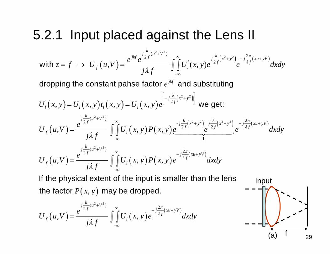
5.2.1 Input placed against the Lens I( )( ),Input: a planar transparency with located imediately in front of the lens

Fourier transformer: a converging lens with focal length Illumination: a uniform (across the transparency , ) normally

At x y

fξ η incident

( ),

1

monochromatic plane wave of amplitude .Disturbance incident on the lens:

inside the lens aperturel A

AU At x y=

⎧( ) 1,

0 inside the lens aperture

Pupil fuunction (for finite extent of the lens): otherwise

Note: here s

P x y⎧

= ⎨⎩

( ) ( ),ince lens is very close to aperture , x yξ η →

( ) ( ) ( )( )2 2-

' 2, , ,Effect of the lens on the phase

The amplitude distribution behind the lens: kj x yf

l lU x y U x y P x y e+

=

InputEffect of the lens on the phase Disturbance at the lens Lens aperture

( , )Disturbance on the back focal plane of the lens: Using the Fresnel diffraction formula from chapter 4:

fU u V

28f(a)

( ) ( ) ( )2 2 2 2 2( )2 2, ( , )k kjkz j x yj x y j

zz zeU x y e U e e d dj z

π ξ ηξ ηλξ η ξ η

λ

∞− ++ +

−∞

⎧ ⎫= ⎨ ⎬

⎩ ⎭∫ ∫

5.2.1 Input placed against the Lens II

( )( ) ( )

2 22 2

( ) 22' 2, ( , )with

kj u V kjkf f j x y j xu yVf f

f le ez f U u V U x y e e dxdy

j f

πλ

λ

+∞ + − +

−∞

= → = ∫ ∫

( ) ( ) ( ) ( )( )2 2

2' , , , ,

dropping the constant pahse factor and substituting

we get:

jkf

kj x yf

l l l l

e

U x y U x y t x y U x y e⎡ ⎤− +⎢ ⎥⎣ ⎦= =

( )2 2( )

2

,

kj u Vf

feU u V

+

= ( ) ( )( ) ( ) ( )2 2 2 2 2-

2 2

1

, ,k kj x y j x y j xu yVf f f

lU x y P x y e e e dxdyj f

πλ

λ

∞ + + − +

−∞∫ ∫

( ) ( ) ( )( )

2 2( ) 22

, , ,

kj u Vf j xu yV

ff l

eU u V U x y P x y e dxdyj f

πλ

λ

+∞ − +

−∞

= ∫ ∫Input

( ),If the physical extent of the input is smaller than the lens the factor may be dP x y

2 2( ) 22

ropped. kj u Vf π+

29f(a)

( ) ( )( )

( ) 22

, ,

jf j xu yV

ff l

eU u V U x y e dxdyj f

πλ

λ

∞ − +

−∞

= ∫ ∫

5.2.1 Input placed against the Lens IIIsome phase factors Fourier transform of the input amplitude transmittance

at frequenciesFocal plane amplitude distribution / /andf u f f v fλ λ= =

( )( )

( )( )

2 2, ( ) 22

, ,

at frequencies Focal-plane amplitude distributionat coordinates i ku V j u V

f j xu yVf

f leU u V U x y e dxdy

j f

πλ

λ

+∞ − +

−∞

= ∫ ∫

/ / and X Yf u f f v fλ λ= =

Conclusion: the complex amplitude of the field in the focal plane of the lens is the Fraunhofer diffraction pattern of the field incident on the lens.Note: here the distance from lens to the observation plane is only fNote: here the distance from lens to the observation plane is only rather than a distance that satisfies the Fraunhofer diffraction criteria.For the cases that only intensity matters (e.g. photography) these two are

f

the same but when we need to pass the focal-plane amplitude distribution from one lens to another optical system (maybe another lens) then we need the phase information as well so the complete is rfU equired.

Inputp p f

( ) ( )( )

222

2 2, ,

q

j xu yV

ff A

AI u V t x y e dxdyf

πλ

λ

∞ − +

−∞

= ∫ ∫

30f(a)

( ),Measuring , the intensity distribution on the focal plane yields power spectrum or energy spectrum of the input.

fI u V

5.2.2 Input Placed in Front of the Lens I( ), .Input: a planar transparency with located in front of the lens at a distance At dξ η

Input

( ),p p p yFourier transformer: a converging lens with focal length Illumination: a uniform (across the transparency) normall

A

f

ξ η

y incident monochromatic plane wave of amplitude .A

( ) ( ){ }

( )

0 , ,

monochromatic plane wave of amplitude . Fourier spectrum of the light transmitted

by the input transparencyFourier spectrum of the light incident on the lens

X Y A

A

F f f At

F f f

ξ η= F

f(b)d

( )

( )

,

,

Fourier spectrum of the light incident on the lens. l X Y

X Y

F f f

H f f ( ) ( )2 2

2 22 1 2 2 1

, X Y

X Y

zj f fj z f fjkzX Y

X Ye f f H f f e e

πλ πλ

λ− − +

− +⎧

+ <⎪= → =⎨⎪0Transfer Function Fresnel approximation for the

of the propagation transfer function of the propagation otherwise⎪⎩

( ) { } ( ) ( ) ( ) ( )2 2

0, , , , X Yj d f fjkzl X Y l A X Y X YF f f U At H f f F f f e e πλξ η − +

⎧ ⎫⎪ ⎪= = =⎨ ⎬⎪ ⎪

F F

( ) ( ) ( )

( )

2 2

2 2 2 2

0

( )

, ,

Input propagation

dropped the constant phaseX Yj d f fl X Y X Y

k kjkz j x y j

F f f F f f e

e

πλ

ξ η

− +

+ +

⎪ ⎪⎩ ⎭

=

⎧ ⎫ ( )2j x yπ ξ η∞

− +

∫ ∫

31

( ) ( )( )2 2, ( , )

j x y jz zeU x y e U e

j zξ η

ξ ηλ

+ +⎧ ⎫= ⎨ ⎬

⎩ ⎭

( )

Fresnel approximation

j x yze d d

ξ ηλ ξ η

+

−∞∫ ∫

( ) 1 inside the lens apertureP il f ti (f fi it t t f th l ) P

⎧⎨

5.2.2 Input Placed in Front of the Lens II( ),

0p

Pupil fuunction (for finite extent of the lens): otherwise

For now we ignore finite extent of the lens. The field distribution at the focal plane with replacing va

P x y⎧

= ⎨⎩

riables x yξ η→ →The field distribution at the focal plane with replacing va

( ) ( ) ( )( )

( )2 2 2 2( ) ( )22 2

, ,,

riables in the Fresnel approximation:

k kj u V j u Vf fj xu yV

f

x yx u y V

e eπλ

ξ η

+ +∞ − +

→ →→ →

∫ ∫( ) ( ) ( )( )

( ) ( )

( )

, / / , 1

, , , ,

with and

S b i

l X Y X Y

ff l l X Y

F f f f u f f v f P x y

e eU u V U x y P x y e dxdy F f fj f j f

λ

λ λ

λ λ−∞

= = =

= =∫ ∫

( ) ( ) ( ) ( )2 2

iX Yj d f fπλ− +Substitute lF f( ) ( ) ( ) ( )

( ) ( ) ( )2 2

2 2

0

( )2

0

, , , :

, ,

into X Y

X Y

j d f fX Y X Y f

kj u Vf

j d f ff X Y

f F f f e U u V

eU u V F f f ef

πλ

πλ

λ

+

+− +

=

=

Input

( ) ( )

( )2 2

0

/ /

1 ( )2

, ,

and X Y

f X Y

f u f f v f

k dj u Vf f

f fj f

e

λ λ

λ= =

⎛ ⎞− +⎜ ⎟

⎝ ⎠

( )( )2j u V

fπ ξ η

λ∞ − +

∫ ∫f(b)d

32

( )

( ),

,Amplitude and phase

Quadratic phase factorof the light at

f

u V

eU u Vj fλ

= ( )( )

/ /

,

Amplitude and phase of the input spectrum at frequencies and X Y

jf

A

f u f f v f

t e d dξ η

λ

λ λ

ξ η ξ η−∞

= =

∫ ∫( )

For special case d f=

5.2.2 Input Placed in Front of the Lens III

2 21 ( )2

2

1

p

The quadratic phase factor k dj u Vf f

f

e⎛ ⎞− +⎜ ⎟

⎝ ⎠ =

( ) ( )( )21, ,

Amplitude and phase of the light Amplitude and phase of the input spectrum

j u Vf

f AU u V t e d dj f

π ξ ηλξ η ξ η

λ

∞ − +

−∞

= ∫ ∫

( ),phase of the light Amplitude and phase of the input spectrum at at frequ V

( )

/ /uencies and

Conclusion: when the input is placed in front focal plane of the lens,

the phase curvature dissapears and is exactly a

X Yf u f f v f

U u V

λ λ= =

( ),the phase curvature dissapears, and is exactly a

Fourier transformation of the inpufU u V

( ),t transparency At ξ η

Input

33f(b)d

5.2.2 Vignetting: limitation of the effective input by the finite lens aperture

Input plane Focal plane

Goal: including effect of the finite extent of the lens using geometrical optical approximation This is valid

η

ξ

y

x

V

u

Input plane Focal plane[-(d/f)u1, -[d/f]V1]

Effective extent of the input

optical approximation. This is valid if is small enough so that the

input is located deep within the F l i ti d

d

i t

z (u1,V1)θ

θ

Fresnel approximation d

1, 1 1 1( ) / , /

istance of the lens.light amplitude at rays with direction cosines u V u f V fξ η= ≈ ≈∑

LensObject

d f

Not all of the rays coming from iput plane at these angles can pas through the lens. Only the ones within the g

( )

eomtrical shadow of the lens on the input plane meet the condition of apssing through the lens.

t b f d f th F i t f f th t ti f thU V( ), at can be found from the Fourier transform of that portion of the input subtended by the projected

fU u V

( ) ( )/ , /

pupil function at angle , centered at

coordinates d u f d V f

θ

ξ η⎡ ⎤= =⎣ ⎦

34

( )( )

( )( )

2 21 22

, , ,

k dj u Vf f j u V

ff A

Ae d dU u V t P u V e d dj f f f

π ξ ηλξ η ξ η ξ η

λ

⎡ ⎤⎛ ⎞− +⎢ ⎥⎜ ⎟ ∞⎝ ⎠⎣ ⎦ − +

−∞

⎛ ⎞= + +⎜ ⎟

⎝ ⎠∫ ∫

5.2.2 Effect of Vignetting on practical design issuesissues• Vignetting is the limitation for the input by the finite lens

aperture. • For a simple Fourier transforming system, vignetting of

the input space is minimized if Input is placed close to the lens– Input is placed close to the lens

– Lens aperture is much larger than the input transparencyp y

• If we are interested only in the Fourier transform of the input object, we should place it right against the lens to

i i i th i ttiminimize the vignetting. • On the other hand if the input transparency is located at

the front focal plane, then the transform relation is not

35

t e o t oca p a e, t e t e t a s o e at o s otaltered by the quadratic phase factor and that may simplify the problem.

5.2.3 Input Placed Behind the Lens I( )Input: a planar transparency with located in front of the rare focal plane oft x y( ),

.

Input: a planar transparency with located in front of the rare focal plane of the lens at a distance Fourier transformer: a converging lens with focal length Illumination: a uniform (across t

At x y

df

he transparency) normally incident monochromaticIllumination: a uniform (across t

( ),

he transparency) normally incident monochromatic plane wave of amplitude .The incident wavefront on the input , is a spherical wave convergingA

At x y

towards the back focal plane of the lens.An approxiamtion based on the following facts: 1) Linear dimension of the cirular bundle at the lens is reduced by a factor

Input

d

( )/ ,of at the input 2) Energy has been conservedAmplitude of the spherical wave im

Ad f t x y

/pinging on the input: Af dl

f(c)( )

/

( / ), /

Illuminated area on the input: is the diameter of the lensThe limitted illumination of the input can be presented by

a pupil function at the input plane

ld f l

P f d f dξ η⎡⎣ ⎤⎦

l

36

( )( / ), /a pupil function at the input plane P f d f dξ η⎡⎣Effective aperture of the system: intersection of the input aperture

with the projected pupil function of the lens on the input plane.

⎤⎦

5.2.3 Input Placed Behind the Lens IIUsing the paraxial approximation for the amplitude of a transmitted wave by a

( ) ( )( )2 2

' 2, ( , ) ,

Using the paraxial approximation for the amplitude of a transmitted wave by a

spherical lens is: we write the amplitude transmitted at the input plane as:

kj x yf

l lU x y U x y P x y e− +

=

( )0 ,

we write the amplitude transmitted at the input plane as:

Af fU Pd d

ξ η ξ ⎛=( ) ( )

2 2

2, ,

Assuming the Fresnel approx for the propagation from the input plane to the focal plane:

kjd

Af e td

ξ ηη ξ η

− +⎧ ⎫⎡ ⎤⎞ ⎛ ⎞⎨ ⎬⎜ ⎟ ⎜ ⎟⎢ ⎥⎝ ⎠ ⎝ ⎠⎣ ⎦⎩ ⎭

( ) ( ) ( )2 2 2 2 2( )2 2, ( , )

Assuming the Fresnel approx. for the propagation from the input plane to the focal plane:k kjkz j x yj x y j

zz zeU x y e U e e d dj z

π ξ ηξ ηλξ η ξ η

λ

∞− ++ +

−∞

⎧ ⎫= ⎨ ⎬

⎩ ⎭∫ ∫ with & &

Th lit d t th f l l b

x u y V z d→ → =

( )( )

( ) ( ) ( ) ( )2 2

2 2 2 2 222 2, , ( ),

The amplitude at the focal plane becomes:kj u V k kd j j j u v

d d df A

e Af f fU u V t P e e e d dj d d d d

πξ η ξ η ξ ηλξ η ξ η ξ η

λ

+ ∞− + + − +

−∞

⎧ ⎫⎡ ⎤⎛ ⎞= ⎨ ⎬⎜ ⎟⎢ ⎥⎝ ⎠⎣ ⎦⎩ ⎭∫ ∫

Input

d( )( )

( )2 2

2, , ( ),

kj u Vd

f AAe f f fU u V t P

j d d d dξ η ξ η

λ

∞

+

⎣ ⎦⎩ ⎭

⎛= ⎜⎝

( )2j u vde d dπ ξ ηλ ξ η

∞− +

−∞

⎧ ⎫⎡ ⎤⎞⎨ ⎬⎟⎢ ⎥⎠⎣ ⎦⎩ ⎭

∫ ∫

37f(c)

Again up to a phase factor, the focal-plane amplitude distribution

of the input transparency is the Fourier transform of the portion of the input subtended by the projected lens aperture.

5.2 Comparison of three casesa) Input in front of the transformer pressed against it:

Input

( ) ( ) ( )( )

2 2( ) 22

, , ,

) p p g

kj u Vf j xu yV

ff A

AeU u V t x y P x y e dxdyj f

πλ

λ

+∞ − +

−∞

= ∫ ∫ f(a)

( ),

b) Input in front of the transformer at a distance from the lens:

fU u V ( ) ( )( )

2 21 ( ) 22

, ,

k dj u Vf f j u V

fA

Ae t P x y e d dπ ξ η

λξ η ξ η

⎛ ⎞− +⎜ ⎟ ∞⎝ ⎠ − +

= ∫ ∫

( )Input

I

( ),Amplitude and phase

f

( )

( ) ( )

, /

, ,

of the light Quadratic phase factor Amplitude and phase of the input spectrum Can be eleiminated by at at frequencies aX

A

d fu V f u f

yj f

λ

ξ η ξ ηλ −∞

= =

∫ ∫

/nd

c) Input in back of the transformer at a distance from the back focal plane of Yf v f

dλ= f(b)d

Inputd

( )( )

( ) ( )2 2

22, , ( ),

the transformer:kj u Vd j u v

df A

Ae f f fU u V t P e d dj d d d d

π ξ ηλξ η ξ η ξ η

λ

+ ∞− +⎧ ⎫⎡ ⎤⎛ ⎞= ⎨ ⎬⎜ ⎟⎢ ⎥⎝ ⎠⎣ ⎦⎩ ⎭

∫ ∫

f(c)

( ) ( ), , ( ),

Th

f Aj d d d dξ η ξ η ξ η

λ −∞

⎨ ⎬⎜ ⎟⎢ ⎥⎝ ⎠⎣ ⎦⎩ ⎭∫ ∫

( ) ( )( )

e results of case a , (b) and c are essentially the same except that

in case c scale of the Fourier transform is determined by the experimenter.

38

( )That is , the distance between input and back focal pland

,e of the lens.

For both (a) and (c) cases give identical results.d f=

5.3 Image Formation: Monochromatic IlluminationIlluminationIf an object in front of a lens illuminated properly, there will be a second plane

across which the field distribution resembles the object.

:The image may be

actual rays intersect to form the imagreal:

e seems like the rays coming from a virtual intensity distribution planevirtual : seems like the rays coming from a virtual intensity distribution plane.

We impose the following limitations on our analysis at this point:

Lenses are positive, aberration-free, and thin th

virtual

1at form real images .z f>

Only monochromatic illumination (implies that the imaging system is linear in

complex amplitutedes). More general case will be trated in chapter 6

Ul U’l UiU0

More general case will be trated in chapter 6.

39z1 z2object System

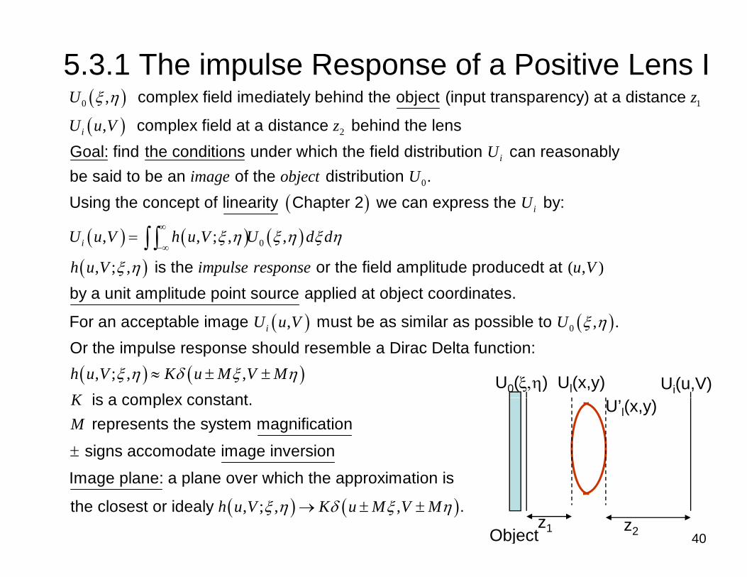
5.3.1 The impulse Response of a Positive Lens I( )0 1, complex field imediately behind the object (input transparency) at a distance U zξ η( )( ) 2, complex field at a distance behind the lens

Goal: find the conditions under which the field distributioniU u V z

0

can reasonably be said to be an of the distribution

iUimage object U

( )

( ) ( ) ( )

0

0

.

, , ; , ,

be said to be an of the distribution Using the concept of linearity Chapter 2 we can express the by:i

i

image object UU

U u V h u V U d dξ η ξ η ξ η∞

−∞= ∫ ∫

( ), ; , is the oh u V impulse responseξ η

( ) ( )0

( , )r the field amplitude producedt at by a unit amplitude point source applied at object coordinates.

For an acceptable image must be as similar as possible to

u V

U u V U ξ η( ) ( )0, , .For an acceptable image must be as similar as possible to Or the impulse response s

iU u V U ξ η

( ) ( ), ; , ,hould resemble a Dirac Delta function:

is a complex constanth u V K u M V MK

ξ η δ ξ η≈ ± ± Ul(x,y) Ui(u,V)U0(ξ,η) is a complex constant. represents the system magnification

signs accomodate image inversion

KM

±

U’l(x,y)

40

Image plane: a plane over which the approximati

( ) ( ), ; , ,

on is

the closest or idealy .h u V K u M V Mξ η δ ξ η→ ± ±z1 z2Object

5.3.1 The impulse Response of a Positive Lens II( )T fi d i l l t th bj t b it lit d i th V ξ( )

( )

, ; ,

( , ) .0

To find impulse response: we let the object be a unit amplitude point

source located at , or U The incident wave on the lens will be a jkr

h u V

er

ξ η

ξ η ξ η =Ul(x,y) Ui(u,V)U0(ξ,η)

spherical wave diverging from the point ξ( )

1

, .

Paraxial approximation to at is: jkre r zr

η

=

U’l(x,y)

( )( )2 2

1

2 2

( )2

1

1,kj x yz

l

k

r

U x y ej z

ξ η

λ

⎡ ⎤− + −⎢ ⎥⎣ ⎦

⎡ ⎤

≈z1 z2

Object

( ) ( )2 2

' 2, , ( , )The field distribution after the lens:

Using Fresnel Diffraction equation to account l

kj x yf

lU x y U x y P x y e⎡ ⎤− +⎣ ⎦=

2

2 :for propagtion over a distance k

z⎡ ⎤( )2 2

2( )

2'

2

1( , ; , ) ( , )

Putting together all:

kj u x V yz

lh u V U x y e dxdyj z

ξ ηλ

⎡ ⎤− + −∞ ⎢ ⎥⎣ ⎦

−∞= ∫ ∫

41

( ) ( )2 22 22 2

1 2( ) ( )

2 222

1 2

1( , ; , ) ( , )k kkj x y j u x V yj x yz zfh u V e P x y e e dxdy

z z

ξ ηξ η

λ

⎡ ⎤ ⎡ ⎤⎡ ⎤− + − − + −− +⎢ ⎥ ⎢ ⎥⎣ ⎦⎣ ⎦ ⎣ ⎦=∞

−∞∫ ∫

5.3.1 The impulse Response of a Positive Lens IIIIntegration is over and so we can pull out all of the terms independent ofx y x y

( ) ( )2 22 22 2

1 2( ) ( )

2 222

1 2

,

1( , ; , ) ( , )

Integration is over and so we can pull out all of the terms independent of k kkj x y j u x V yj x yz zf

x y x y

h u V e P x y e e dxdyz z

ξ ηξ η

λ

⎡ ⎤ ⎡ ⎤⎡ ⎤− + − − + −− +∞ ⎢ ⎥ ⎢ ⎥⎣ ⎦⎣ ⎦ ⎣ ⎦

−∞= ∫ ∫

Neglecting a pure phase 2 2 2 2

2 12 22

1( , ; , )

factor we get:k kj u V jz zh u V e e

ξ ηξ η

⎡ ⎤ ⎡ ⎤+ +⎣ ⎦ ⎣ ⎦=

( )2 2

1 2 1 2 1 2

21 2

1 1 12

( , ; , )

( , ) k u Vj x y jk x y

z z f z z z z

h u V e ez z

P x y e e dxdyξ η

ξ ηλ

⎡ ⎤ ⎡ ⎤⎛ ⎞ ⎛ ⎞ ⎛ ⎞+ − + − + + +⎢ ⎥ ⎢ ⎥⎜ ⎟ ⎜ ⎟ ⎜ ⎟∞ ⎢ ⎥ ⎢ ⎥⎝ ⎠ ⎝ ⎠ ⎝ ⎠⎣ ⎦ ⎣ ⎦

∞× ∫ ∫

this result together with

iU u

−∞∫ ∫

( ) ( ) ( )0, , ; , ,V h u V U d dξ η ξ η ξ η∞

= ∫ ∫Ul(x,y)

U’l(x,y)

Ui(u,V)U0(ξ,η)

( ) ( ) ( )( ) ( )( ) ( )

0

0

, , .

, ,

enable us to calculate if we know

But when we can say is image of i

i

U u V U

U u V U

ξ η

ξ η

−∞∫ ∫

42

is difficult unless we do further simplifications.z1 z2

Object

5.3.2 Eliminating Quadratic Phase Factors: The Lens Law IThe Lens Law I

2 2 2 2

2 12 21( ; )

Let's look at the troublesome terms of the impulse response mainly quadratic factors:k kj u V jz zh u V e e

ξ ηξ η

⎡ ⎤ ⎡ ⎤+ +⎣ ⎦ ⎣ ⎦2 1

21 2

( , ; , )

(

independent of the lens coordinates

h u V e ez z

P x

ξ ηλ

=

×( )2 2

1 2 1 2 1 2

1 1 12, )k u Vj x y jk x y

z z f z z z zy e e dxdyξ η⎡ ⎤ ⎡ ⎤⎛ ⎞ ⎛ ⎞ ⎛ ⎞

+ − + − + + +⎢ ⎥ ⎢ ⎥⎜ ⎟ ⎜ ⎟ ⎜ ⎟∞ ⎢ ⎥ ⎢ ⎥⎝ ⎠ ⎝ ⎠ ⎝ ⎠⎣ ⎦ ⎣ ⎦∞∫ ∫

1 2

1 1 12

Depends on the lens coordinates

Approximations that will elliminate these factors:

1)kj x

z z f

−∞

⎛ ⎞+ −⎜ ⎟

⎝ ⎠

∫ ∫

( )2 2

effect of this term will be broadening of the impulse responsey

⎡ ⎤+⎢ ⎥

⎢ ⎥⎣ ⎦1 21) fe ⎝ ⎠

12

( , ; , ) ( , ). effect of this term will be broadening of the impulse response.

Without that will be a pure Fourier transformation of the

So if we choose a distance that the termkj

h u V P x y

e

ξ η

⎢ ⎥⎣ ⎦

( )2 2

1 2

1 1

( ; )vanishes thenx y

z z f h u V ξ η⎡ ⎤⎛ ⎞

+ − +⎢ ⎥⎜ ⎟⎢ ⎥⎝ ⎠⎣ ⎦So if we choose a distance that the term e

1 2

( , ; , )1 1 1 0

1 1 1

vanishes then

would be the closest approximation of the impulse response. So let

h u V

z z f

ξ η⎝ ⎠⎣ ⎦

+ − =

43

1 2

1 1 1 0The classical of the geometrical optics: has lens lawz z f+ − = to

be satisfied for image formation.

5.3.2 Eliminating Quadratic Phase Factors: The Lens Law IIThe Lens Law II

2 2 2 2

1 22 21( ) ( )

Impulse response after application of the :uk k jk xj u V j z z zz z

lens law

hξ η

ξ ηξ

⎛ ⎞− + +⎡ ⎤ ⎡ ⎤ ⎜ ⎟+ +⎣ ⎦ ⎣ ⎦ ⎝ ⎠ 1 2

V yz d d

⎡ ⎤⎛ ⎞+⎢ ⎥⎜ ⎟∞ ⎢ ⎥⎝ ⎠⎣ ⎦∫ ∫ 1 22 12 2

21 2

1( , ; , ) ( , )Depends on the Depends only on image location the object location

z z zz zh u V e e P x y ez z

ξ ηλ

⎣ ⎦ ⎣ ⎦ ⎝ ⎠= 1 2

Approximations that will elliminate these factors:

z dxdy⎢ ⎥⎝ ⎠⎣ ⎦

−∞∫ ∫

2 2

222) can be ignored under two conditions: a) if we are only interested in the intensity at the

kj u Vze⎡ ⎤+⎣ ⎦

Ul(x,y)

U’l(x,y)

Ui(u,V)U0(ξ,η)

object plane

2 2

, then phase distribution is

unimportant. most of the time this is the case k ⎡ ⎤ zObject

R=z2

2 2

22and we drop the factor.b) The image is measured on a shperical surface with radius centered at the point

kj u Vze

z

⎡ ⎤+⎣ ⎦

where the

z1 z2Object

The surface on which th d ti h

44

2with radius , centered at the pointz where the optical axis pierces the thin lens.

the quadratic phase factor on u and V is zero

5.3.2 Eliminating Quadratic Phase Factors IIII l ft li ti f th d li i ti thl l

2 2

21

Impulse response after application of the and eliminating the quadratic phase factor dependent on the image coordinates:

kj

lens law

ξ η⎡ ⎤+⎣ ⎦u Vjk x yξ η⎡ ⎤⎛ ⎞ ⎛ ⎞

− + + +⎢ ⎥⎜ ⎟ ⎜ ⎟∞ ⎢ ⎥⎝ ⎠ ⎝ ⎠⎣ ⎦∫ ∫122

1 2

1( , ; , )Depends only on the object location

jzh u V e

z z

ξ ηξ η

λ⎣ ⎦

= 1 2 1 2

2 2

2

( , ) z z z z

kj

P x y e dxdy

ξ η

∞ ⎢ ⎥⎝ ⎠ ⎝ ⎠⎣ ⎦

−∞

⎡ ⎤+⎣ ⎦

∫ ∫

( ) ( ) ( )

12

;

3) this term will affect the image severly through the convolution operation in calculating the image:

jze

U u V h u V U

ξ η

ξ η ξ η

⎣ ⎦

∞= ∫ ∫ d dξ η( ) ( ) ( )0, , ; , ,iU u V h u V Uξ η ξ η

−∞= ∫ ∫ .

Under 3 conditions this term can be ignored: 3.a) the object exists on a shperical surface

d dξ η

Ul(x,y)

U’l(x,y)

Ui(u,V)U0(ξ,η)

1with radius , centered on the point where the optical axis pierces the thin lens. This rarely happens

z

in reality. R=z2R=z1

45

This rarely happens in reality.z1 z2

Object

5.3.2 Eliminating Quadratic Phase Factors IVImpulse response after application of the and quadratic phaselens law

2 2

1121( ; ) ( )

Impulse response after application of the and quadratic phase factor dependent on the image coordinates:

k jkj zz

lens law

h u V e P x y eξ

ξ ηξ η

− +⎡ ⎤+⎣ ⎦= 2 1 2

u Vx yz z z dxdy

η⎡ ⎤⎛ ⎞ ⎛ ⎞+ +⎢ ⎥⎜ ⎟ ⎜ ⎟∞ ⎢ ⎥⎝ ⎠ ⎝ ⎠⎣ ⎦∫ ∫2

1 2

( , ; , ) ( , )Depends only on the object location

h u V e P x y ez z

ξ ηλ

3.b) the object is illuminated by a spherical wave that is converging towards the point

dxdy−∞∫ ∫

Ui(u,V)U0(ξ,η)

wave that is converging towards the point that optical axis pierces the lens. A proper illumination can make this happen. The spherical wave illumination results in Fourier transform of the object apear in the pupil plane of the lens.The quadratic phase factor will cancell by the quadratuic phase factor of this

z1 z2Object

( )1

2 2

-This term with conversion of

and and

converging spherical wave (simmilar to the case of transparency behind the lens:

u V d z

kj u V

ξ η→ → →

+⎧ ⎫⎡ ⎤

46

( )( )

( )22

, , ( ),j u V

d jd

f AA e f f fU u V t P e

j d d d d

πλξ η ξ η

λ

+−⎧ ⎫⎡ ⎤⎛ ⎞= ⎨ ⎬⎜ ⎟⎢ ⎥⎝ ⎠⎣ ⎦⎩ ⎭

( )u vd d

ξ ηξ η

∞+

−∞∫ ∫

5.3.2 Eliminating Quadratic Phase Factors VImpulse response after application of the and quadratic phase lens law

2 2

1122

1 2

1( , ; , ) ( , )Depends only

factor dependent on the image coordinates:k jkj zzh u V e P x y e

z z

ξξ η

ξ ηλ

− +⎡ ⎤+⎣ ⎦= 2 1 2

u Vx yz z z dxdy

η⎡ ⎤⎛ ⎞ ⎛ ⎞+ +⎢ ⎥⎜ ⎟ ⎜ ⎟∞ ⎢ ⎥⎝ ⎠ ⎝ ⎠⎣ ⎦

−∞∫ ∫(u,V)(ξ,η)

1 2 Depends only on the object location

z zλ

3.c) The phase of the quadratic factor changes by an amount that is only a small fraction of a radian within the region of the object that contributes signifi

( )( )

,

,

cantlyto the field at the particular image point .

This is true most of the time, otherwise the image at would be very blurred.

u V

u V

z1 z2Object

( )2 2

12

,, g y

In that case the can be replaced by a single phaskjze

ξ η⎡ ⎤+⎣ ⎦ e that depends on the coordinates of the image point of the interest but not the object point.

2 22 2

211 22 2

1

g j

where is the magnification of the system.

N thi

k u Vk jj z Mz ze e Mz

ξ η⎡ ⎤+

⎡ ⎤ ⎢ ⎥+⎣ ⎦ ⎢ ⎥⎣ ⎦→ = −

h f t b d d if i t t d l i i t it

47

Now this new p

14

hase factor can be dropped if we are interested only in intesity.

Practical examination shows that this holds for: object size (lens aperture size)<

5.3.2 Eliminating Quadratic Phase Factors( ) ( ) ( )0, , ; , ,iU u V h u V U d dξ η ξ η ξ η

∞

−∞= ∫ ∫

( )2 22 2 2 2

1 22 1

1 1 122 2

21 2 2 3

1( , ; , ) ( , )Approximation Approximation Depends on the lens coordinates

Lens law took

kk k j x yj u V j z z fz zh u V e e P x y ez z

ξ ηξ η

λ

∞

⎡ ⎤⎛ ⎞+ − +⎡ ⎤ ⎡ ⎤ ⎢ ⎥⎜ ⎟+ +⎣ ⎦ ⎣ ⎦ ⎢ ⎥⎝ ⎠⎣ ⎦=

∫ ∫1 2 1 2

care of it

R lt f ll f th i ti th i l f thi iti h i l l i

u Vjk x yz z z ze dxdyξ η⎡ ⎤⎛ ⎞ ⎛ ⎞

− + + +⎢ ⎥⎜ ⎟ ⎜ ⎟∞ ⎢ ⎥⎝ ⎠ ⎝ ⎠⎣ ⎦−∞∫ ∫

1

21 2

1( , ; , ) ( , )

Result of all of the approximations on the impulse response of a thin, positive, spherical lens is:

jkzh u V P x y e

z z

ξ

ξ ηλ

−

≈ 2 1 2

h i h

u Vx yz z z dxdy

η⎡ ⎤⎛ ⎞ ⎛ ⎞+ + +⎢ ⎥⎜ ⎟ ⎜ ⎟∞ ⎢ ⎥⎝ ⎠ ⎝ ⎠⎣ ⎦

−∞∫ ∫

( ) ( )2

2 12

1 2

/

1 1( , ; , ) ( , )

together with

h th l l i li d th t th i l f thi l

j u M x V M yz

M z z

h u V P x y e dxdyz z

π ξ ηλξ η

λ λ

− ⎡ − + − ⎤∞ ⎣ ⎦

−∞

= −

≈ ∫ ∫i th F h fwhen the lens law is applied we see that the impulse response of a thin lens

1

1 ,

is the Fraunhofer

diffraction pattern of the lens aperture, apart from a scaling factor of centered on the

image coordinates of The simplifications used to arrive at this conclusion az

u M V Mλ

ξ η= = re:, .image coordinates of The simplifications used to arrive at this conclusion au M V Mξ η= =

1 21/ 1/ 1/

re:

1) Lens law holds 2) Only intensity of image matters or the image plane is spherical with the radius of curvature

equal to the image-lens distance.

z z f+ =

48

equal to the image lens distance.

3) Object is on a spherical surface

1/ 4

or illumination is done by a spherical wave converging with

radius of curvature equal to the object-lens distance or object size of the lens aperture size.<

5.3.3 The Relation Between Object and ImageFor a perfect imaging system, image is a magnified/demagnified replica of the object.

( ) 01, ,

In Geometrical optics image and object are related by:

iu VU u V U

M M M⎛ ⎞= ⎜ ⎟⎝ ⎠

We can show that the wave optics image

( ) ( )2

21 1lim ( ; ) lim ( )

reduces to the geometrical optics image as 0. Start from impulse response (approximate form) of a positive lens:

j u M x V M yzh u V P x y e dxdyπ ξ η

λ

λ

ξ η− ⎡ − + − ⎤∞ ⎣ ⎦

→

≈ ∫ ∫ 2

0 01 2

lim ( , ; , ) lim ( , )

Change variables:

h u V P x y e dxdyz zλ λ

ξ ηλ λ −∞→ →

≈ ∫ ∫

( ) ( )

2 2

2 ' '2

' / , ' /

lim ( ; ) lim ( ' ' ) ' '

j u M x V M y

x x z y y zzh u V P x z y z e dx dyπ ξ η

λ λ

ξ η λ λ∞ − ⎡ − + − ⎤⎣ ⎦

= =

≈ ∫ ∫ 2 10 01

2 1

lim ( , ; , ) lim ( , )

0 ( ' , ' )As the aperture function gets wider. So at the limit the aperture is infinitly wide. We

h u V P x z y z e dx dyz

P x z y z

λ λξ η λ λ

λ λ λ

−∞→ →≈

→

∫ ∫

2 1/can replace it with 1. Difining M z z=

( ) ( )

( ) ( )

2 ' '

0 0

1lim ( , ; , ) lim 1. ' ' ,

lim ( ; )

Fourier transform of unity

we get: j u M x V M y u Vh u V M e dx dyM M M

U V h V U

π ξ η

λ λξ η δ ξ η

ξ η ξ η

∞ − ⎡ − + − ⎤⎣ ⎦−∞→ →

∞

⎛ ⎞≈ ≈ − −⎜ ⎟⎝ ⎠∫ ∫

∫ ∫ d dξ η

49

( ) ( )00, lim ( , ; , ) ,iU u V h u V U

λξ η ξ η

−∞ →= ∫ ∫

( ) ( ) ( )0 01 1, , , , ,i i

d d

u V u VU u V U d d U u V UM M M M M M

ξ η

δ ξ η ξ η ξ η∞

−∞

⎛ ⎞ ⎛ ⎞= − − → =⎜ ⎟ ⎜ ⎟⎝ ⎠ ⎝ ⎠∫ ∫

Effect of diffraction on the relation between object and image Iobject and image I

( ) ( )2

2

1 2

1 1( , ; , ) ( , )

Impulse response of the imaging system: j u M x V M y

zh u V P x y e dxdyz z

π ξ ηλξ η

λ λ

− ⎡ − + − ⎤∞ ⎣ ⎦

−∞≈ ∫ ∫

1 2

This is impulse response of a linear space-variant system. So the object and image are related by a su

z zλ λ

perposition integral not a convolution. The space-variant atribute is due to magnification and inversion To transform this relationship to a convolution:magnification and inversion. To transform this relationship to a convolution:change to a normalized set of object-plane var

( ) ( )2

2

2

,

1( , ; , ) ( , )

iables: j u x V y

z

M M

h u V P x y e dxdyπ ξ η

λ

ξ ξ η η

ξ ηλ

⎡ ⎤− − + −∞ ⎣ ⎦

∞

= =

= ∫ ∫

( )2

1 2

,This relation has a convolution form which depends on only

Another set of normalizing coordinates for further sim

z z

u V

λ

ξ η

−∞

− −

∫ ∫

1plification: x yx y h h= = =Another set of normalizing coordinates for further sim

( ) ( )

2 2

22 2

, ,| |

( , ; , ) | | ( , ) | |

1

plification:

j u x V y

x y h hz z M

h u V M P z x z y e dxdy M hπ ξ η

λ λ

ξ η λ λ

ξ

∞ ⎡ ⎤− − + −⎣ ⎦−∞

= =

⎡ ⎤⎛ ⎞

∫ ∫

50

( ) ( )( )

0

,

1, , ,

image from Geometrical optics analysisg

i

U u V

U u V h u V UM M M

ξ ηξ η⎡ ⎤⎛ ⎞

= − − ⎢ ⎥⎜ ⎟⎢ ⎥⎝ ⎠⎣ ⎦

d dξ η∞

−∞∫ ∫

Effect of diffraction on the relation between object and image II( ) ( ) ( ) ( ) 0

1, , , , ,Effect of diffraction Image by

where i g gU u V h u V U u V U u V UM M M

ξ η⎛ ⎞= ⊗ = ⎜ ⎟

⎝ ⎠

object and image II

( )

g yon the image Geometrical optics

analysis

The point-spead function introduced by diffraction is then:

( ) ( )2 1j ux Vy x yπ∞ ⎡ + ⎤⎣ ⎦∫ ∫( ) 2, ,h u V P z xλ λ= ( ) ( )22

2 2

1, ,| |

where

Conclusions: 1) The ideal image produced by a diffraction limitted optical system (free

j ux Vy x yz y e dxdy x y h hz z M

π

λ λ⎡− + ⎤⎣ ⎦

−∞= = =∫ ∫

1) The ideal image produced by a diffraction-limitted optical system (freefrom aberrations) is scaled and inverted version of the object.2) The effect of diffraction is to convolve that ideal image with the

Fraunhofer diffraction pattern of the lens pupil.Convolution smooths the image and attenuates the fine details of the object.We will talk about applications of filtering to imaging systems in chapter 6

51

We will talk about applications of filtering to imaging systems in chapter 6.

5.4 Analysis of Complex Coherent Optical SystemsSystems• A certain “operator” notation will be useful to analyze

complicated optical systems with many lenses and free-space regions.

52

5.4.1 An operator notation

Several operator approaches has been introduced to analyze complicated optical systems. We follow the approach introduced by Nazarathy and Shamir:

Simplifying assumption: 1) Monochromatic systems.2) Coherent systems.) y3) Only paraxial conditions will be considered.4) One-dimensional treatment of the system good for the problems that their aperture function is separable in rectangular coordinatesaperture function is separable in rectangular coordinates.Opar

[ ]{ }ator: represents a fundamental operation of the system.

Notation: Operator parameters dependent on the geometry Quantity

53

5.4.1 The basic operators useful to us

[ ] ( ){ } ( )2

21)

Four operators that are sufficient to analyze most optical systems:

Multiplication by a quadratic phase exponential: kj cx

c U x e U x=Q

[ ] [ ]12 / ,

2)

Where and is an inverse length and

Scaling by

k c c cπ λ −= = −Q Q

[ ] ( ){ } ( )1/ 2 a constant: b U x b U bx=V { }[ ] [ ]

( ){ } ( ) ( )

1

2

1/

3)

Where is dimensionless and

Fourier transformation: j fx

b b b

U x U x e dx G fπ

−

∞ −

=

= =∫

V V

F ( ){ } ( ) ( )

( ){ } ( ) ( ){ } ( )

{ } ( )22 1

1 2 1

)

1

and j fx

kj x x

f

G f U f e df U x U xπ

−∞

∞− −

−∞

− −

= =

∫∫F FF

∞

∫[ ] ( ){ } ( ) ( )2 121 1

14) Free space propagation: j x x

dd U x U x e dxj dλ

=R 1

2Where distance of propagation, coordinate after propagation.d x

∞

−∞

= =

∫

54

[ ] [ ]1 -d d− =R R

5.4.1 Relationship among the basic operators [ ] [ ] [ ][ ] [ ] [ ]

[ ]

[ ]

2 1 2 1

1 a statement of the similarity theorem of the Fourier analysis

t t t t

tt

=

⎡ ⎤= ⎢ ⎥⎣ ⎦

V V V

FV V F

[ ][ ] [ ] [ ][ ]

2 1 2 1

1 2

1 follows from the Fourier inversion theorem

Free propagation in

c c c c

d dλ−

= −

= +

⎡ ⎤= −⎣ ⎦

FF V

Q Q Q

R F Q F space can be analyzed by Fresnel [ ] ⎣ ⎦

[ ] [ ] [ ]

diffraction or by a series of Fourier transformation, multiplication by a quadraticphase factor, and inverse Fourier transformation.

b h bc⎡ ⎤Q V V Q iti th d fi iti[ ] [ ] [ ] 2 can be shown by wcc t tt⎡ ⎤= ⎢ ⎥⎣ ⎦

Q V V Q

[ ] 1 1 1

riting the definitions

Fresnel diffraction operation is equivalent to dd d dλ⎡ ⎤ ⎡ ⎤ ⎡ ⎤= ⎢ ⎥ ⎢ ⎥ ⎢ ⎥⎣ ⎦ ⎣ ⎦ ⎣ ⎦

R Q V FQ

multiplication by a quadratic phase factor, properly scaled Fourier transform,followed by multipl

⎣ ⎦ ⎣ ⎦ ⎣ ⎦

[ ] [ ]1 1

ication by a quadratic-phase exponential.

f f⎡ ⎤ ⎡ ⎤⎢ ⎥ ⎢ ⎥V F R Q R

55

[ ] [ ]

Fields across the front and back focal planes of a positive lens are related by a properly scaled Fourier transform with no quadrati

f ff fλ

= −⎢ ⎥ ⎢ ⎥⎣ ⎦ ⎣ ⎦

V F R Q R

c phase exponential.

Relations between the basic operators

d⎡ ⎤ ⎡ ⎤

V F Q R

[ ] [ ] [ ] [ ] [ ] [ ] [ ] [ ] [ ] [ ]

[ ] [ ] [ ] [ ]

22 1 2 1 2

22

1

1 1

dt t t t t t c t c t t d tt t

ct c d dt

λλ

⎡ ⎤ ⎡ ⎤⎡ ⎤= = = =⎣ ⎦⎢ ⎥ ⎢ ⎥⎣ ⎦ ⎣ ⎦⎡ ⎤ ⎡ ⎤ ⎡ ⎤= = − = − = −⎣ ⎦⎢ ⎥ ⎢ ⎥⎣ ⎦ ⎣ ⎦

V V V V V F FV V Q Q V V R R V

F FV V F FF V Q F FR FR Q F

[ ] [ ] [ ] [ ] [ ] [ ] [ ][ ] [ ] ( )

[ ] ( )

11

2 1 2 12 2 111

c d d cc cc t t c c c c ct cd c dλ

−−

−−

⎣ ⎦ ⎣ ⎦⎡ ⎤= +⎢ ⎥⎣ ⎦⎡ ⎤ ⎡ ⎤= = − = +⎢ ⎥ ⎢ ⎥⎣ ⎦ ⎣ ⎦ ⎡⋅ + ⋅ +

⎣

Q R RQ Q V V Q Q F FR Q Q Q

V Q ⎤⎢ ⎥⎦⎣

[ ] [ ] [ ] [ ][ ] [ ] ( )

( ) ( )[ ] [ ] [ ]

11

2 21 2 1 211 11

d c c dd t t t d d d d d d d

cd d cλ

−−

−− −

⎦⎡ ⎤= +⎢ ⎥⎣ ⎦⎡ ⎤ ⎡ ⎤= = − = +⎣ ⎦ ⎣ ⎦ ⎡ ⎤⎡ ⎤⋅ + ⋅ +⎢ ⎥⎣ ⎦ ⎣ ⎦

R Q QR R V V R R F FQ R R R

V R⎣ ⎦

56

5.4.2 Application of the Operator Approach to Some Optical Systems Ito Some Optical Systems I

2 1

1

Example 1) Two spherical lenses each with focal length of and separation of Goal: to determione the relationship between the complex field across and .

f fS S

⎡ ⎤ 1⎡ ⎤1

Le

The reletionship operator: f

⎡ ⎤= −⎢ ⎥

⎣ ⎦S Q [ ] 1

1 1 1

Propagationns 2 Lens 1

ff

⎡ ⎤−⎢ ⎥⎣ ⎦

⎡ ⎤ ⎡ ⎤ ⎡ ⎤

R Q

[ ] 1 1 1

1 1 1 1 1 1 1 1 1

We can simplify the using

using

dd d d

f f f f f f f f f

λ

λ

⎡ ⎤ ⎡ ⎤ ⎡ ⎤= ⎢ ⎥ ⎢ ⎥ ⎢ ⎥⎣ ⎦ ⎣ ⎦ ⎣ ⎦⎡ ⎤ ⎡ ⎤ ⎡ ⎤ ⎡ ⎤ ⎡ ⎤ ⎡ ⎤ ⎡ ⎤ ⎡ ⎤ ⎡

= − − − = −⎢ ⎥ ⎢ ⎥ ⎢ ⎥ ⎢ ⎥ ⎢ ⎥ ⎢ ⎥ ⎢ ⎥ ⎢ ⎥ ⎢⎣ ⎦ ⎣ ⎦ ⎣ ⎦ ⎣ ⎦ ⎣ ⎦ ⎣ ⎦ ⎣ ⎦ ⎣ ⎦ ⎣

S R Q V FQ

S Q Q V FQ Q Q Q Q Q 1⎤=⎥

⎦g

f f f f f f f f fλ⎢ ⎥ ⎢ ⎥ ⎢ ⎥ ⎢ ⎥ ⎢ ⎥ ⎢ ⎥ ⎢ ⎥ ⎢ ⎥ ⎢⎣ ⎦ ⎣ ⎦ ⎣ ⎦ ⎣ ⎦ ⎣ ⎦ ⎣ ⎦ ⎣ ⎦ ⎣ ⎦ ⎣

Q Q Q Q Q Q Q Q

1 11 1 this is equivalent to a scaled Fourier transform f fλ λ

⎥⎦

⎡ ⎤ ⎡ ⎤= ⋅ ⋅ → =⎢ ⎥ ⎢ ⎥

⎣ ⎦ ⎣ ⎦S V F S V F

without a quadratic phase factor. This is similar to the focal-plane-to-focal-plane relationship seen earlier:

1 kj xu−∞

∫

Sl S2f

57

fU ( ) ( )01

12

Field just to Field just to the left of Lthe right of L

jfu U x e dx

fλ∞

−∞= ∫

L1 L2

5.4.2 Application of the Operator Approach to Some Optical Systems IIto Some Optical Systems II

1 1( ).Example 2) An input transparency located at a distance from a converging lens with focal length of illuminated by a point source located at a distance from the lens Location of the outpu

df z z d>

2t of interest : on the plane of image of the point source. Where thezLocation of the outpu

[ ] [ ]

2

1 2

21

1/ 1/ 1/

1 1

t of interest : on the plane of image of the point source. Where the usual lens law holds

zz z f

z df z d

+ =

⎡ ⎤⎡ ⎤= − ⎢ ⎥⎢ ⎥ −⎣ ⎦ ⎣ ⎦

S R Q R Q

d

1PropagationPropagationEffect of the Input is illuminatlens

f z d⎣ ⎦ ⎣ ⎦ed by a diverging

spherical wave that affects it by a quadratic phase factor

Applying the the lens law: z2z1

[ ] [ ]

[ ] [ ] ( ) ( )

21 2 1

11

1 1 1

1

Using the table we simplify thisz dz z z d

d c c d cd−−

⎡ ⎤ ⎡ ⎤= − −⎢ ⎥ ⎢ ⎥−⎣ ⎦ ⎣ ⎦

⎡ ⎤= + ⋅ +⎢ ⎥⎣ ⎦

S R Q R Q

R Q Q V ( ) 11 1d c−− −⎡ ⎤⎡ ⎤ ⋅ +⎢ ⎥⎣ ⎦ ⎣ ⎦

R[ ] [ ] ( ) ( )1d c c d cd+ +⎢ ⎥⎣ ⎦R Q Q V ( )

[ ]1 1 1

1 2 22 2

1 2 1 2 1 2 1 2

1 1 1 1 11 1

d c

z z zz zz z z z z z z z

− − −

+⎢ ⎥⎣ ⎦ ⎣ ⎦⎡ ⎤ ⎡ ⎤ ⎡ ⎤⎡ ⎤ ⎛ ⎞ ⎛ ⎞ ⎛ ⎞⎢ ⎥ ⎢ ⎥ ⎢ ⎥− − = − + − − − −⎜ ⎟ ⎜ ⎟ ⎜ ⎟⎢ ⎥ +⎢ ⎥ ⎢ ⎥ ⎢ ⎥⎣ ⎦ ⎝ ⎠ ⎝ ⎠ ⎝ ⎠⎣ ⎦ ⎣ ⎦ ⎣ ⎦

R

R Q Q V R

58

[ ] [ ]1 2 12 12

1 2 2 2

1 1 z z zz zz z z z

⎡ ⎤⎡ ⎤ ⎛ ⎞ ⎡ ⎤+− − = − −⎢ ⎥⎜ ⎟⎢ ⎥ ⎢ ⎥⎣ ⎦ ⎝ ⎠ ⎣ ⎦⎣ ⎦

R Q Q V R

5.4.2 Application of the Operator Approach to Some Optical Systems III

[ ] [ ] [ ]1 2 1 1 2 11 12 2

2 2 1 2 2 1

1 1z z z z z zz d d zz z z d z z z d

⎡ ⎤ ⎡ ⎤⎛ ⎞ ⎡ ⎤ ⎡ ⎤ ⎛ ⎞ ⎡ ⎤ ⎡ ⎤+ += − − = − −⎢ ⎥ ⎢ ⎥⎜ ⎟ ⎜ ⎟⎢ ⎥ ⎢ ⎥ ⎢ ⎥ ⎢ ⎥− −⎝ ⎠ ⎣ ⎦ ⎣ ⎦ ⎝ ⎠ ⎣ ⎦ ⎣ ⎦⎣ ⎦ ⎣ ⎦

⎡ ⎤ ⎡ ⎤ ⎡ ⎤

S Q V R R Q Q V R Q

Approach to Some Optical Systems III

[ ] [ ]

[ ] ( )

1

1

1 1 1

1 1

Next we use to simplify d d zd d d

d zd d

λ

λ

⎡ ⎤ ⎡ ⎤ ⎡ ⎤= −⎢ ⎥ ⎢ ⎥ ⎢ ⎥⎣ ⎦ ⎣ ⎦ ⎣ ⎦⎡ ⎤⎡ ⎤

− = ⎢ ⎥⎢ ⎥⎢ ⎥⎣ ⎦

R Q V FQ R

R Q V F1

d⎡ ⎤⎢ ⎥⎣ ⎦

Q[ ] ( )11 1d z d zλ⎢ ⎥⎢ ⎥− −⎢ ⎥⎣ ⎦ ⎣ ⎦

( )

1

1 2 122 2 1 1 1 1

1 1 1 1

d z

z z zz z d z d z d z z dλ

⎢ ⎥−⎣ ⎦

⎡ ⎤⎡ ⎤ ⎡ ⎤ ⎡ ⎤ ⎡ ⎤ ⎡ ⎤+= − ⎢ ⎥⎢ ⎥ ⎢ ⎥ ⎢ ⎥ ⎢ ⎥ ⎢ ⎥− − − −⎢ ⎥⎣ ⎦ ⎣ ⎦ ⎣ ⎦ ⎣ ⎦ ⎣ ⎦⎣ ⎦

S Q V Q V FQ Q

( )

1

1 2 122 2 1 1

1 1z z zz z d z d zλ

⎡ ⎤⎡ ⎤ ⎡ ⎤ ⎡ ⎤+= − ⎢ ⎥⎢ ⎥ ⎢ ⎥ ⎢ ⎥− −⎢ ⎥⎣ ⎦ ⎣ ⎦ ⎣ ⎦ ⎣ ⎦

⎡ ⎤

S Q V Q V F

[ ] [ ] [ ] 2Finaly using we flip cc t tt⎡ ⎤= ⎢ ⎥⎣ ⎦

Q V V Q

( ) ( )2

1 2 1 12 2

1

the orders of and

z z z zd dλ

⎡ ⎤ ⎡ ⎤⎡ ⎤ ⎡ ⎤+= −⎢ ⎥ ⎢ ⎥⎢ ⎥ ⎢ ⎥

⎢ ⎥ ⎢ ⎥⎣ ⎦ ⎣ ⎦

Q V

S Q Q V V F

59

( ) ( )

( ) ( )

2 22 2 1 2 1

21 2 1 1

2 22 2 1 2 1

1

z z d z z d z

z z z zz z d z z d z

λ

λ

⎢ ⎥ ⎢ ⎥⎢ ⎥ ⎢ ⎥− −⎢ ⎥ ⎢ ⎥⎣ ⎦ ⎣ ⎦⎣ ⎦ ⎣ ⎦⎡ ⎤ ⎡ ⎤+

= + −⎢ ⎥ ⎢ ⎥− −⎢ ⎥ ⎢ ⎥⎣ ⎦ ⎣ ⎦

S Q V F

5.4.2 Application of the Operator Approach to Some Optical Systems IV

( )( ) ( )

( ) ( )

1 2 1 2 122 1 2 1

:Comparing this to the conventional relation ship between and

d z z z z zz d z z z d

U U u

λ

ξ

⎡ ⎤ ⎡ ⎤+ −= ⎢ ⎥ ⎢ ⎥

− −⎢ ⎥ ⎢ ⎥⎣ ⎦ ⎣ ⎦S Q V F

Approach to Some Optical Systems IV

( ) ( )

( )

( )( )

( )( ) ( )

1 2 1 22 12 1

2 1

1 2

22

2 1

:Comparing this to the conventional relation ship between and z z d z zkj zz d z j u

z z d

U U u

eU u U e dd

π ξλ

ξ

ξ ξλ

⎡ ⎤+ −⎢ ⎥ ⎡ ⎤− ∞⎢ ⎥ −⎣ ⎦ ⎢ ⎥

−⎢ ⎥⎣ ⎦= ∫( )2 1

1Fourie

z z dz

λ −∞− ∫r transform of the input amplitude distribution

with a scaling factor

Some results from this example that are more general than just this example:) F i t f l d t t b th f l l f th l th ta) Fourier transform plane need not to be the focal plane of the lens that

performs the transformation.b) Fourier trnsform always appears in the plane where the source is imaged.) Q d ti h f t di th F i t f ti i lc) Quadratic-phase factor preceding the Fourier transform operation is always

the quadratic-phase factor that would result at the transform plane from a pointsource of light located on the optical axis in the plane of input transparency.

60

Operator technique allows a more mathematical analysis of the complicated systems but it is more abstract than the diffraction integrals and furthere awayfrom the physical analysis.