lec16 partially prestressed concrete beams
DESCRIPTION
lectureTRANSCRIPT
PRESTRESSED CONCRETE STRUCTURES
Amlan K. Sengupta, PhD PE
Department of Civil Engineering
Indian Institute of Technology Madras
Module – 3: Analysis of Members
Lecture – 16: Analysis of Partially Prestressed Sections, Analysis of Behavior
Welcome back to prestressed concrete structures. This is the sixth lecture in module three
on analysis of members. In today’s lecture, we shall study analysis of members under
flexure, specifically for the ultimate strength of partially prestressed sections and
unbonded post-tensioned beams. We shall also look into the analysis of behavior of
members.
First, we are studying the analysis of partially prestressed sections.
(Refer Slide Time 01:46)
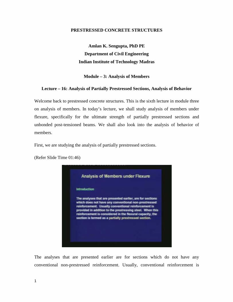
The analyses that are presented earlier are for sections which do not have any
conventional non-prestressed reinforcement. Usually, conventional reinforcement is
1
provided in addition to the prestressing steel. When this reinforcement is considered in
the flexural capacity, the section is termed as a partially prestressed section.
(Refer Slide Time: 02:12)
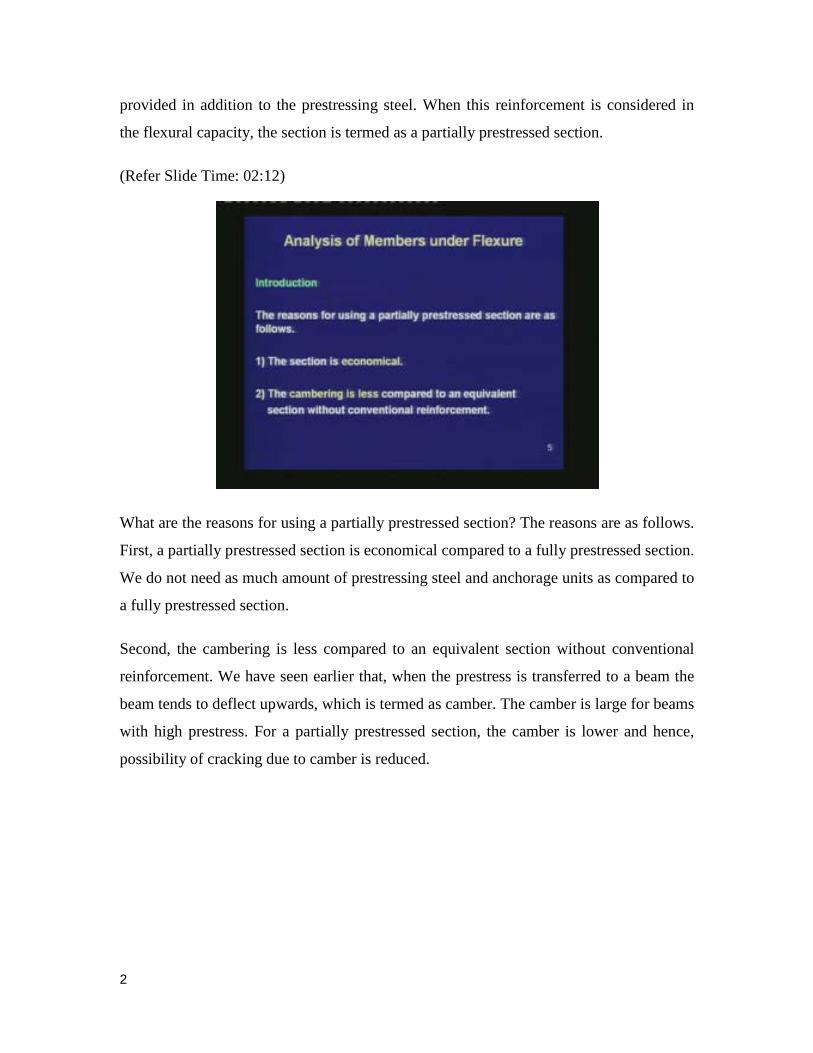
What are the reasons for using a partially prestressed section? The reasons are as follows.
First, a partially prestressed section is economical compared to a fully prestressed section.
We do not need as much amount of prestressing steel and anchorage units as compared to
a fully prestressed section.
Second, the cambering is less compared to an equivalent section without conventional
reinforcement. We have seen earlier that, when the prestress is transferred to a beam the
beam tends to deflect upwards, which is termed as camber. The camber is large for beams
with high prestress. For a partially prestressed section, the camber is lower and hence,
possibility of cracking due to camber is reduced.
2
(Refer Slide Time 03:43)
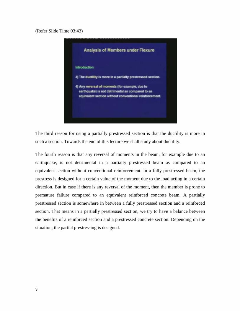
The third reason for using a partially prestressed section is that the ductility is more in
such a section. Towards the end of this lecture we shall study about ductility.
The fourth reason is that any reversal of moments in the beam, for example due to an
earthquake, is not detrimental in a partially prestressed beam as compared to an
equivalent section without conventional reinforcement. In a fully prestressed beam, the
prestress is designed for a certain value of the moment due to the load acting in a certain
direction. But in case if there is any reversal of the moment, then the member is prone to
premature failure compared to an equivalent reinforced concrete beam. A partially
prestressed section is somewhere in between a fully prestressed section and a reinforced
section. That means in a partially prestressed section, we try to have a balance between
the benefits of a reinforced section and a prestressed concrete section. Depending on the
situation, the partial prestressing is designed.
3
(Refer Slide Time: 05:16)
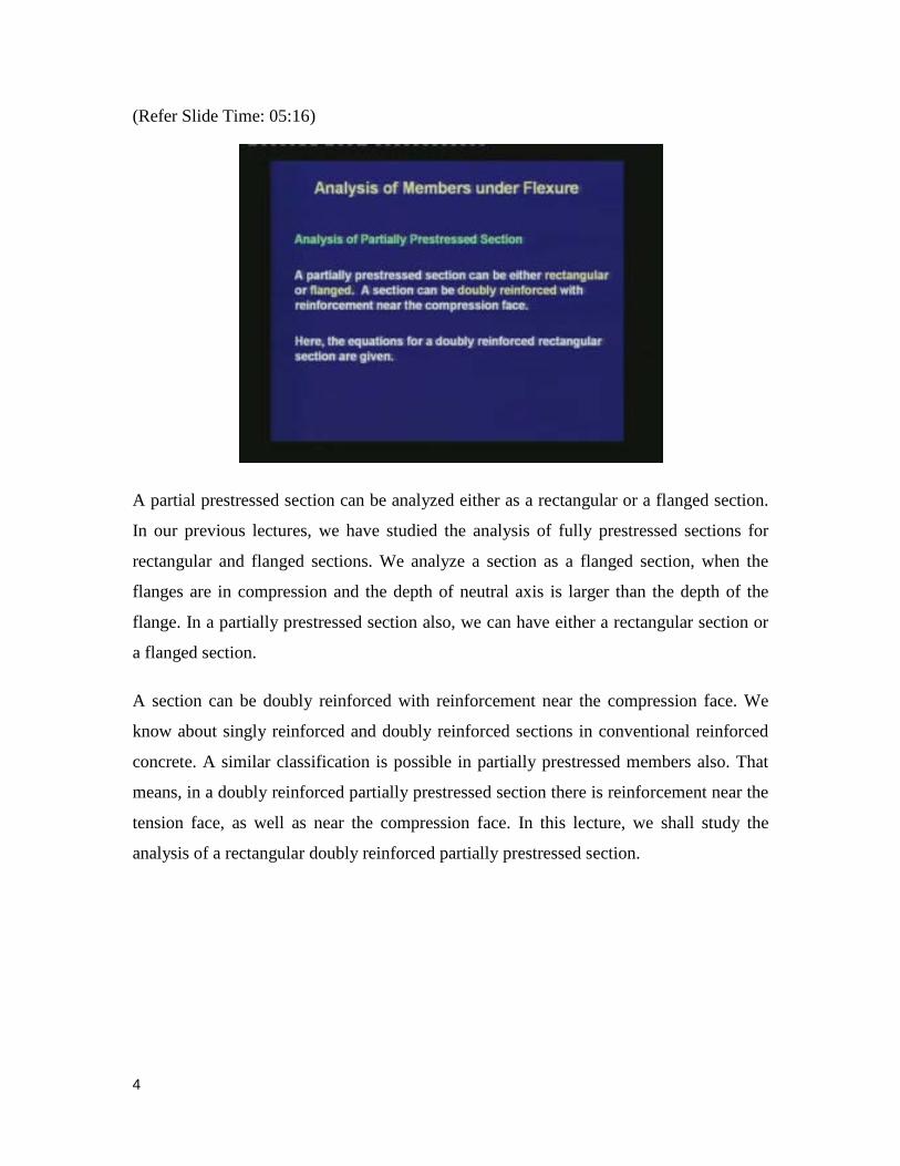
A partial prestressed section can be analyzed either as a rectangular or a flanged section.
In our previous lectures, we have studied the analysis of fully prestressed sections for
rectangular and flanged sections. We analyze a section as a flanged section, when the
flanges are in compression and the depth of neutral axis is larger than the depth of the
flange. In a partially prestressed section also, we can have either a rectangular section or
a flanged section.
A section can be doubly reinforced with reinforcement near the compression face. We
know about singly reinforced and doubly reinforced sections in conventional reinforced
concrete. A similar classification is possible in partially prestressed members also. That
means, in a doubly reinforced partially prestressed section there is reinforcement near the
tension face, as well as near the compression face. In this lecture, we shall study the
analysis of a rectangular doubly reinforced partially prestressed section.
4
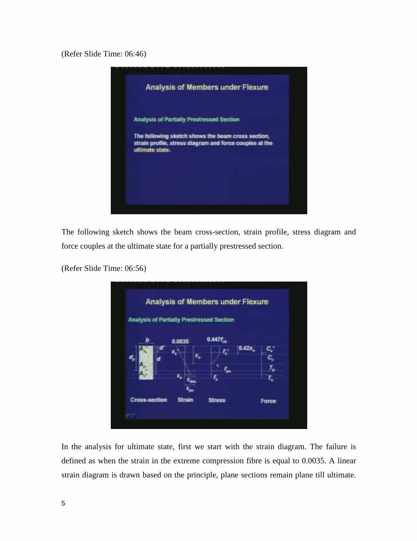
(Refer Slide Time: 06:46)
The following sketch shows the beam cross-section, strain profile, stress diagram and
force couples at the ultimate state for a partially prestressed section.
(Refer Slide Time: 06:56)
In the analysis for ultimate state, first we start with the strain diagram. The failure is
defined as when the strain in the extreme compression fibre is equal to 0.0035. A linear
strain diagram is drawn based on the principle, plane sections remain plane till ultimate.
5
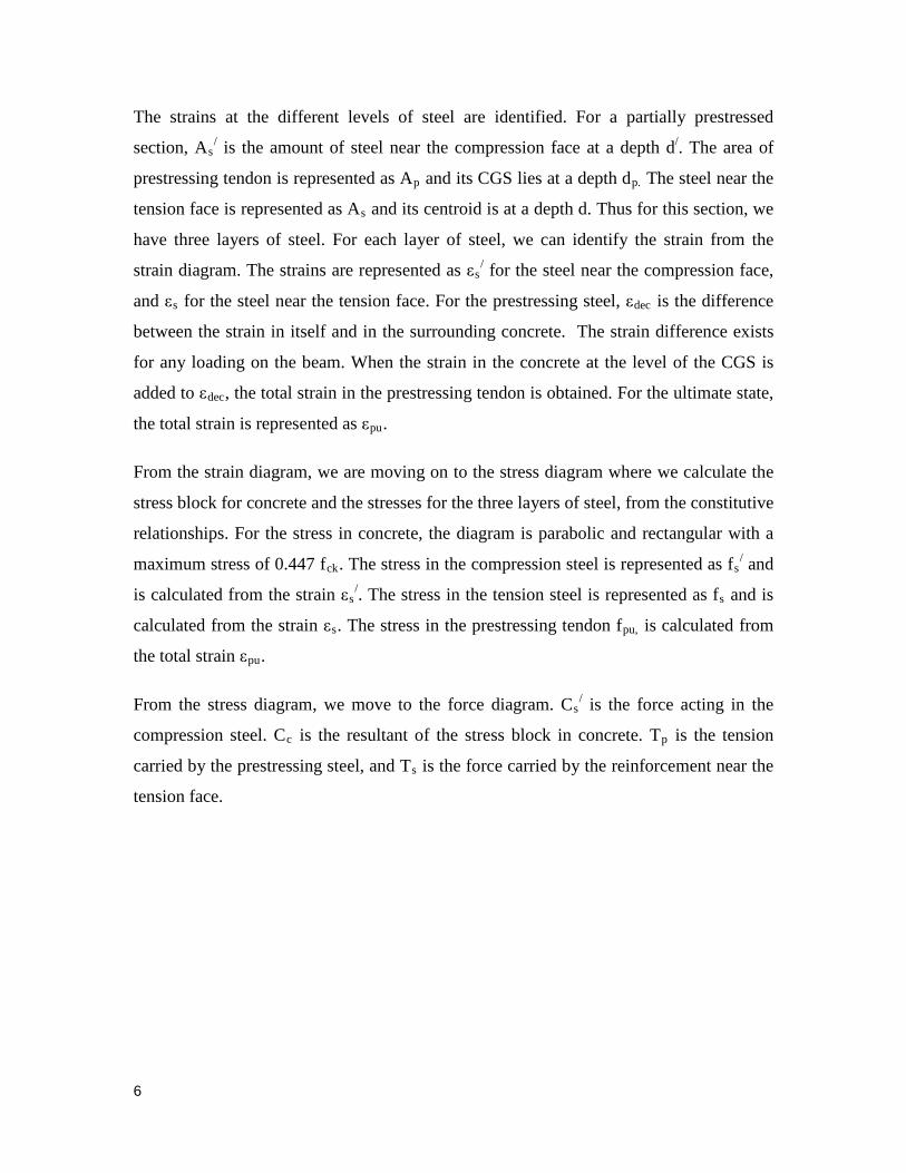
The strains at the different levels of steel are identified. For a partially prestressed
section, As/ is the amount of steel near the compression face at a depth d/. The area of
prestressing tendon is represented as Ap and its CGS lies at a depth dp. The steel near the
tension face is represented as As and its centroid is at a depth d. Thus for this section, we
have three layers of steel. For each layer of steel, we can identify the strain from the
strain diagram. The strains are represented as εs/ for the steel near the compression face,
and εs for the steel near the tension face. For the prestressing steel, εdec is the difference
between the strain in itself and in the surrounding concrete. The strain difference exists
for any loading on the beam. When the strain in the concrete at the level of the CGS is
added to εdec, the total strain in the prestressing tendon is obtained. For the ultimate state,
the total strain is represented as εpu.
From the strain diagram, we are moving on to the stress diagram where we calculate the
stress block for concrete and the stresses for the three layers of steel, from the constitutive
relationships. For the stress in concrete, the diagram is parabolic and rectangular with a
maximum stress of 0.447 fck. The stress in the compression steel is represented as fs/ and
is calculated from the strain εs/. The stress in the tension steel is represented as fs and is
calculated from the strain εs. The stress in the prestressing tendon fpu, is calculated from
the total strain εpu.
From the stress diagram, we move to the force diagram. Cs/ is the force acting in the
compression steel. Cc is the resultant of the stress block in concrete. Tp is the tension
carried by the prestressing steel, and Ts is the force carried by the reinforcement near the
tension face.
6
(Refer Slide Time: 10:47)
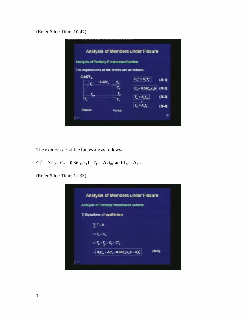
The expressions of the forces are as follows:
Cs/ = As
/fs/, Cc = 0.36fckxub, Tp = Apfpu and Ts = Asfs.
(Refer Slide Time: 11:33)
7
Next, we write the equations based on the principles of mechanics. First, let us start with
the equations of equilibrium. For the longitudinal forces, ΣF = 0, which gives the total
tension is equal to the total compression. The tension constitutes of Tp, the tension in the
prestressing tendon, and Ts which is the tension in the reinforcement steel near the
tension face. The compression also consists of two components, Cc which is the
component taken by the concrete and Cs/ which is the compression taken by the
compression steel. We are writing the expressions of the individual forces, and this gives
us the first equilibrium equation.
(Refer Slide Time: 12:35)
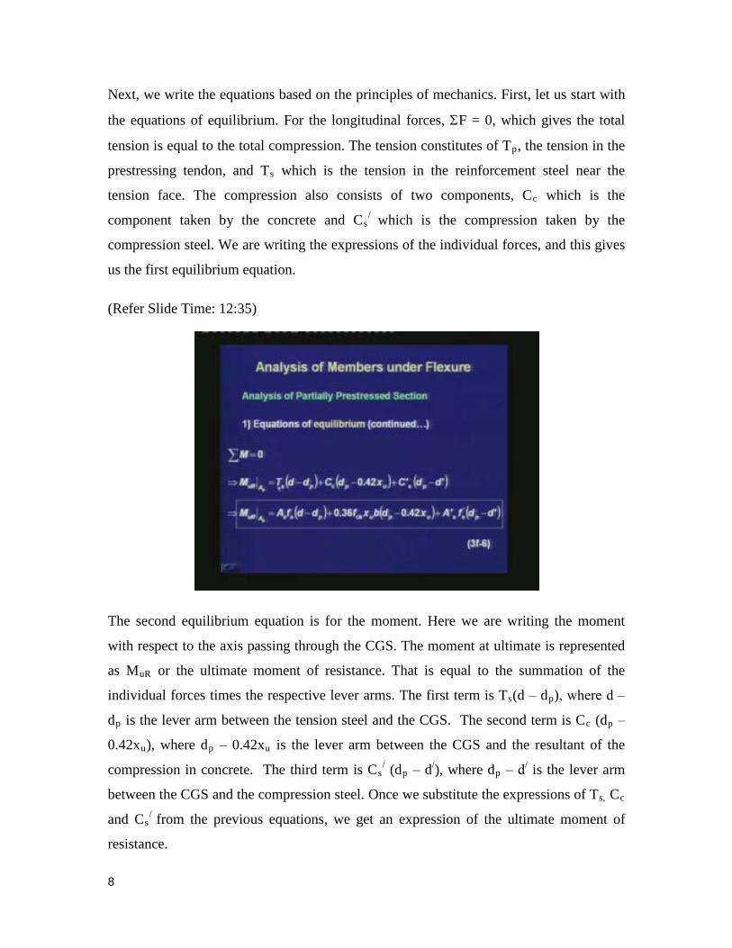
The second equilibrium equation is for the moment. Here we are writing the moment
with respect to the axis passing through the CGS. The moment at ultimate is represented
as MuR or the ultimate moment of resistance. That is equal to the summation of the
individual forces times the respective lever arms. The first term is Ts(d ‒ dp), where d ‒
dp is the lever arm between the tension steel and the CGS. The second term is Cc (dp ‒
0.42xu), where dp ‒ 0.42xu is the lever arm between the CGS and the resultant of the
compression in concrete. The third term is Cs/ (dp ‒ d/), where dp ‒ d/ is the lever arm
between the CGS and the compression steel. Once we substitute the expressions of Ts, Cc
and Cs/ from the previous equations, we get an expression of the ultimate moment of
resistance.
8
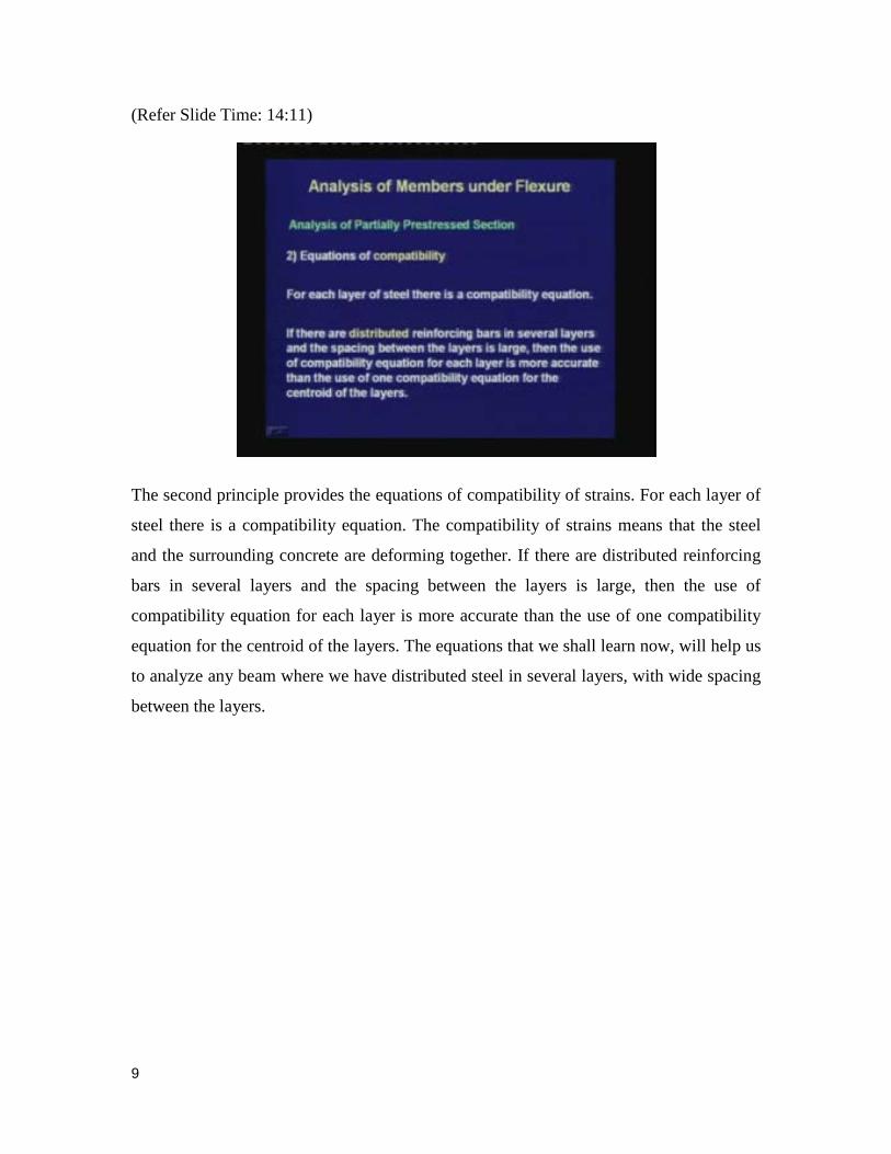
(Refer Slide Time: 14:11)
The second principle provides the equations of compatibility of strains. For each layer of
steel there is a compatibility equation. The compatibility of strains means that the steel
and the surrounding concrete are deforming together. If there are distributed reinforcing
bars in several layers and the spacing between the layers is large, then the use of
compatibility equation for each layer is more accurate than the use of one compatibility
equation for the centroid of the layers. The equations that we shall learn now, will help us
to analyze any beam where we have distributed steel in several layers, with wide spacing
between the layers.
9
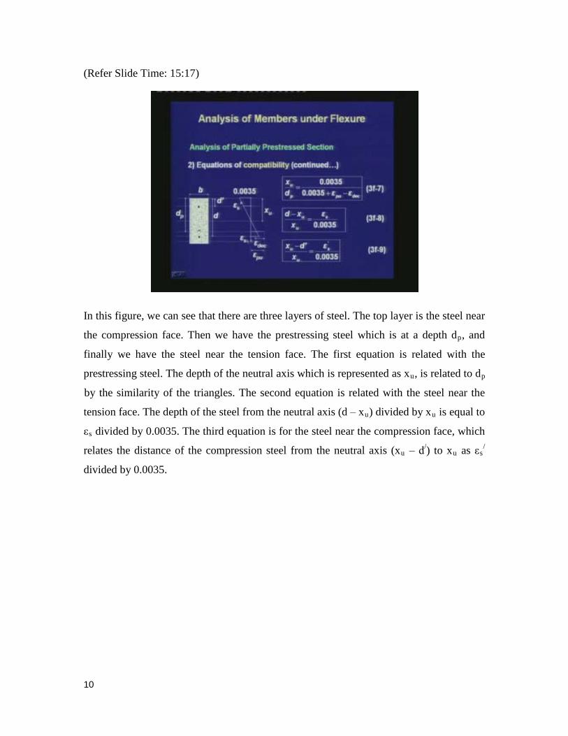
(Refer Slide Time: 15:17)
In this figure, we can see that there are three layers of steel. The top layer is the steel near
the compression face. Then we have the prestressing steel which is at a depth dp, and
finally we have the steel near the tension face. The first equation is related with the
prestressing steel. The depth of the neutral axis which is represented as xu, is related to dp
by the similarity of the triangles. The second equation is related with the steel near the
tension face. The depth of the steel from the neutral axis (d ‒ xu) divided by xu is equal to
εs divided by 0.0035. The third equation is for the steel near the compression face, which
relates the distance of the compression steel from the neutral axis (xu ‒ d/) to xu as εs/
divided by 0.0035.
10
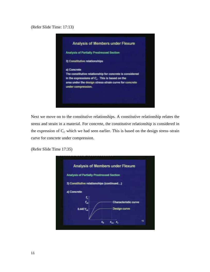
(Refer Slide Time: 17:13)
Next we move on to the constitutive relationships. A constitutive relationship relates the
stress and strain in a material. For concrete, the constitutive relationship is considered in
the expression of Cc which we had seen earlier. This is based on the design stress‒strain
curve for concrete under compression.
(Refer Slide Time 17:35)
11
The design curve has a maximum stress of 0.447fck, and the maximum strain εcu is equal
to 0.0035. When we calculate the area of the stress block, we get the expression of Cc
equal to 0.36fckxub.
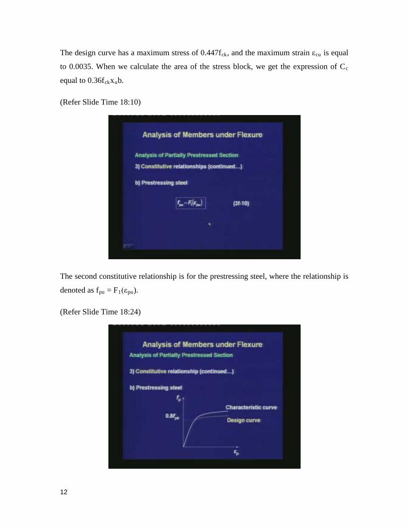
(Refer Slide Time 18:10)
The second constitutive relationship is for the prestressing steel, where the relationship is
denoted as fpu = F1(εpu).
(Refer Slide Time 18:24)
12
This function is available from the design curve for the prestressing steel.
(Refer Slide Time 18:35)
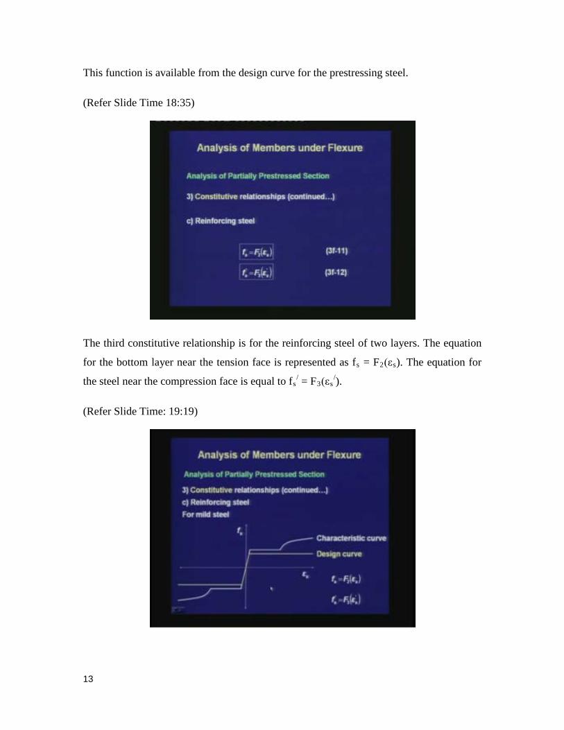
The third constitutive relationship is for the reinforcing steel of two layers. The equation
for the bottom layer near the tension face is represented as fs = F2(εs). The equation for
the steel near the compression face is equal to fs/ = F3(εs
/).
(Refer Slide Time: 19:19)
13
Both the functions F2 and F3 are same, if we are using the same grade of steel for the
bottom steel and the top steel. For mild steel bars, the design curve is an elasto-plastic
curve without any strain hardening.
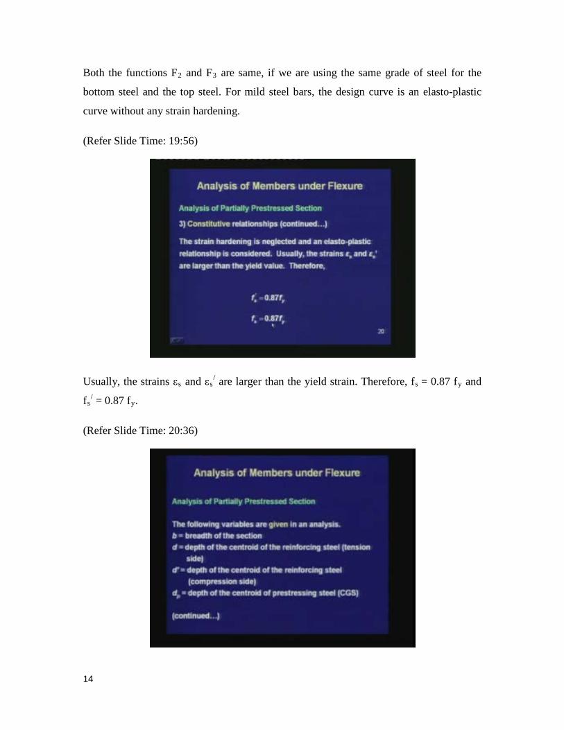
(Refer Slide Time: 19:56)
Usually, the strains εs and εs/ are larger than the yield strain. Therefore, fs
= 0.87 fy and
fs/ = 0.87 fy.
(Refer Slide Time: 20:36)
14
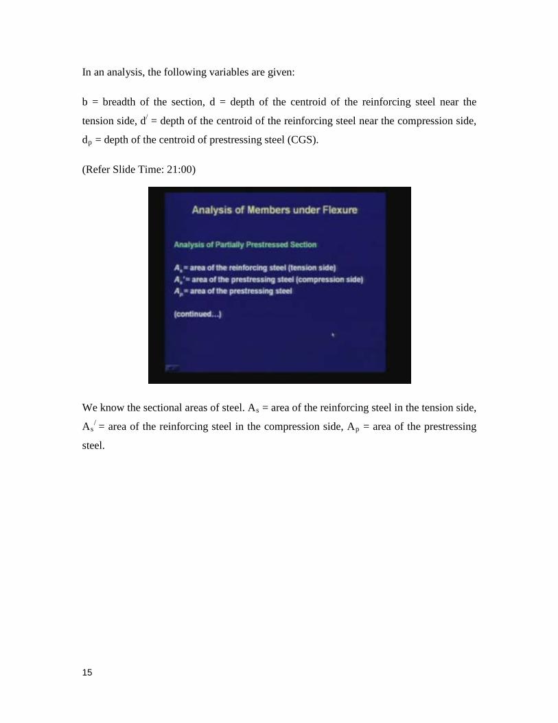
In an analysis, the following variables are given:
b = breadth of the section, d = depth of the centroid of the reinforcing steel near the
tension side, d/ = depth of the centroid of the reinforcing steel near the compression side,
dp = depth of the centroid of prestressing steel (CGS).
(Refer Slide Time: 21:00)
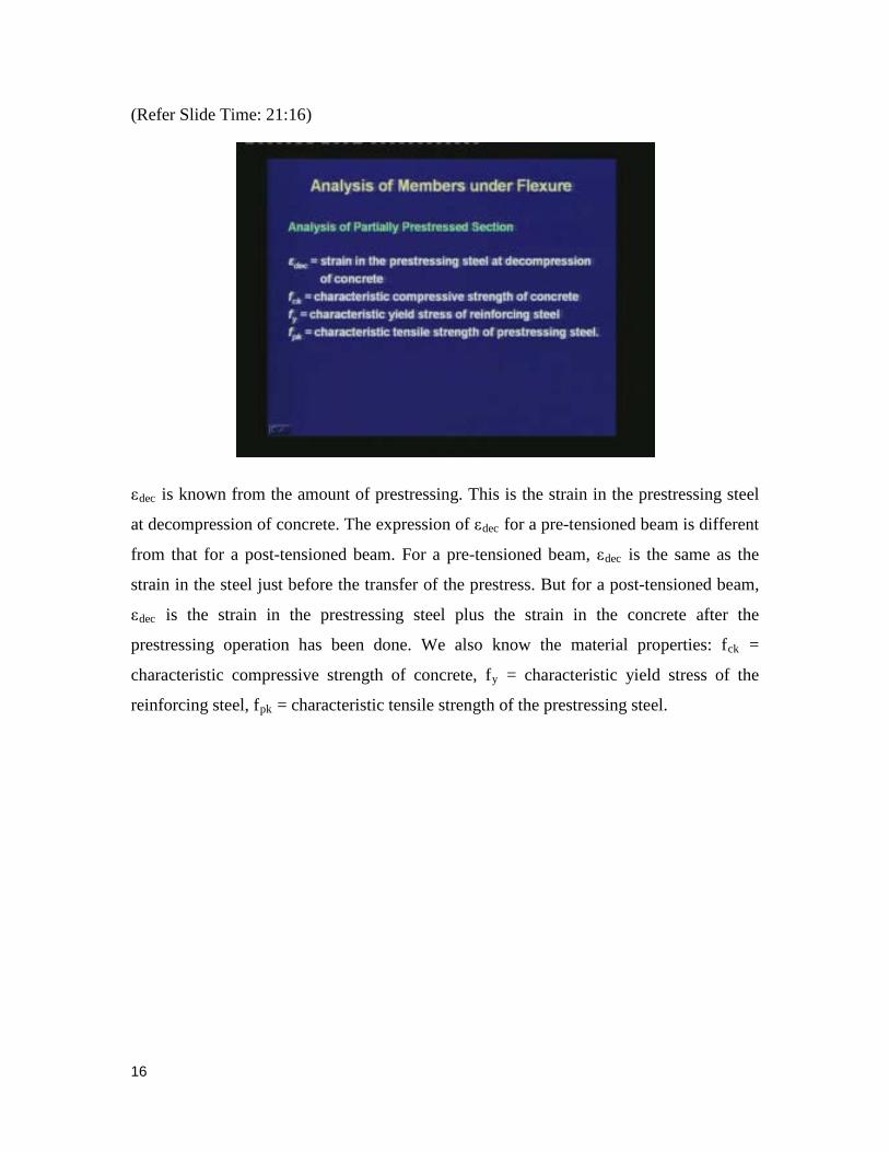
We know the sectional areas of steel. As = area of the reinforcing steel in the tension side,
As/ = area of the reinforcing steel in the compression side, Ap = area of the prestressing
steel.
15
(Refer Slide Time: 21:16)
εdec is known from the amount of prestressing. This is the strain in the prestressing steel
at decompression of concrete. The expression of εdec for a pre-tensioned beam is different
from that for a post-tensioned beam. For a pre-tensioned beam, εdec is the same as the
strain in the steel just before the transfer of the prestress. But for a post-tensioned beam,
εdec is the strain in the prestressing steel plus the strain in the concrete after the
prestressing operation has been done. We also know the material properties: fck =
characteristic compressive strength of concrete, fy = characteristic yield stress of the
reinforcing steel, fpk = characteristic tensile strength of the prestressing steel.
16
(Refer Slide Time: 22:22)
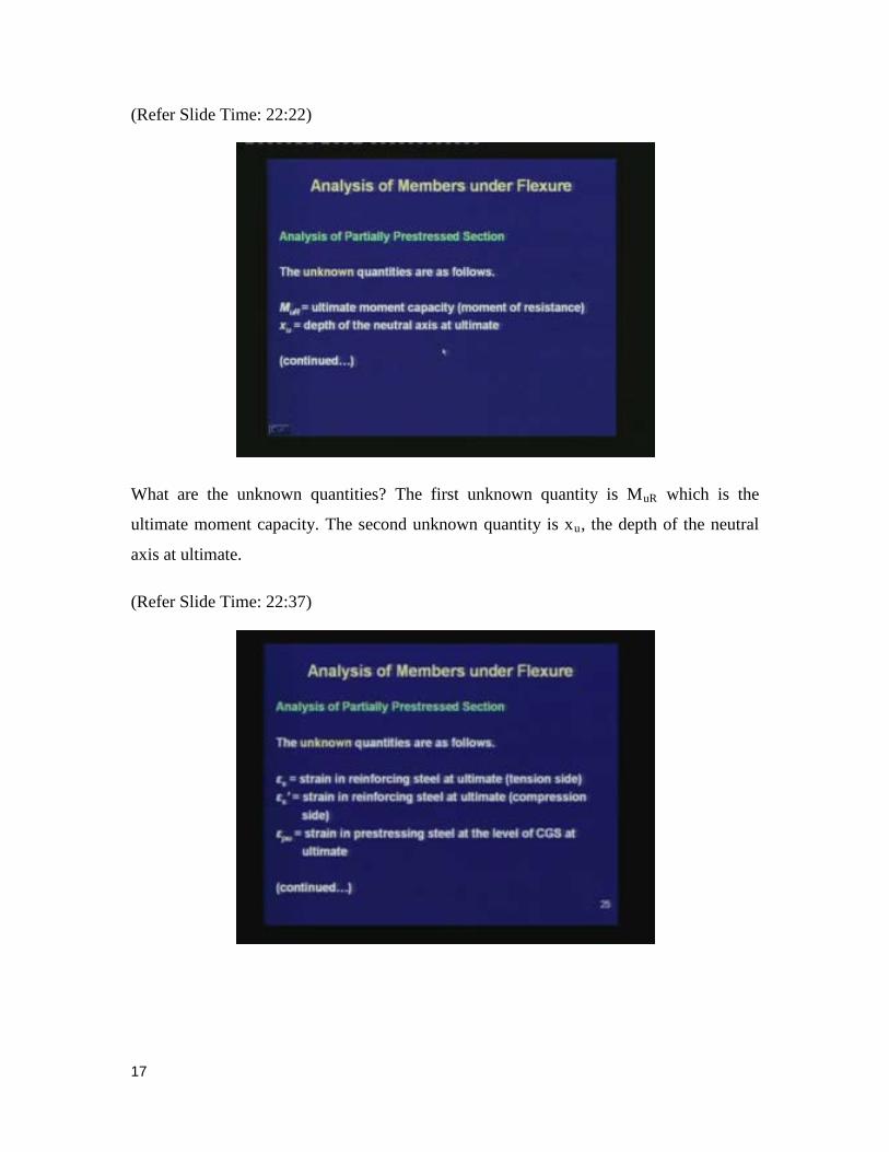
What are the unknown quantities? The first unknown quantity is MuR which is the
ultimate moment capacity. The second unknown quantity is xu, the depth of the neutral
axis at ultimate.
(Refer Slide Time: 22:37)
17
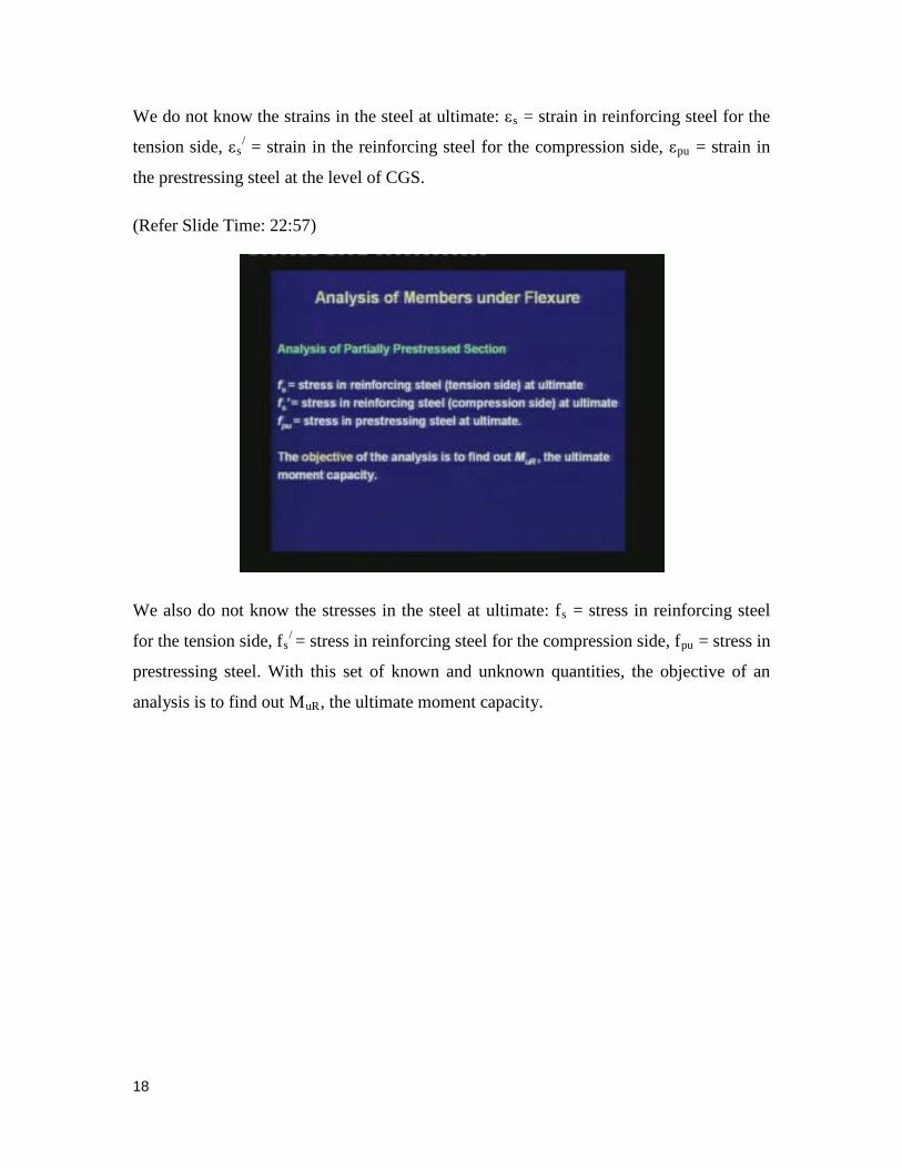
We do not know the strains in the steel at ultimate: εs = strain in reinforcing steel for the
tension side, εs/ = strain in the reinforcing steel for the compression side, εpu = strain in
the prestressing steel at the level of CGS.
(Refer Slide Time: 22:57)
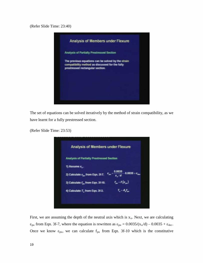
We also do not know the stresses in the steel at ultimate: fs = stress in reinforcing steel
for the tension side, fs/ = stress in reinforcing steel for the compression side, fpu = stress in
prestressing steel. With this set of known and unknown quantities, the objective of an
analysis is to find out MuR, the ultimate moment capacity.
18
(Refer Slide Time: 23:40)
The set of equations can be solved iteratively by the method of strain compatibility, as we
have learnt for a fully prestressed section.
(Refer Slide Time: 23:53)
First, we are assuming the depth of the neutral axis which is xu. Next, we are calculating
εpu from Eqn. 3f-7, where the equation is rewritten as εpu = 0.0035/(xu/d) ‒ 0.0035 + εdec.
Once we know εpu, we can calculate fpu from Eqn. 3f-10 which is the constitutive
19
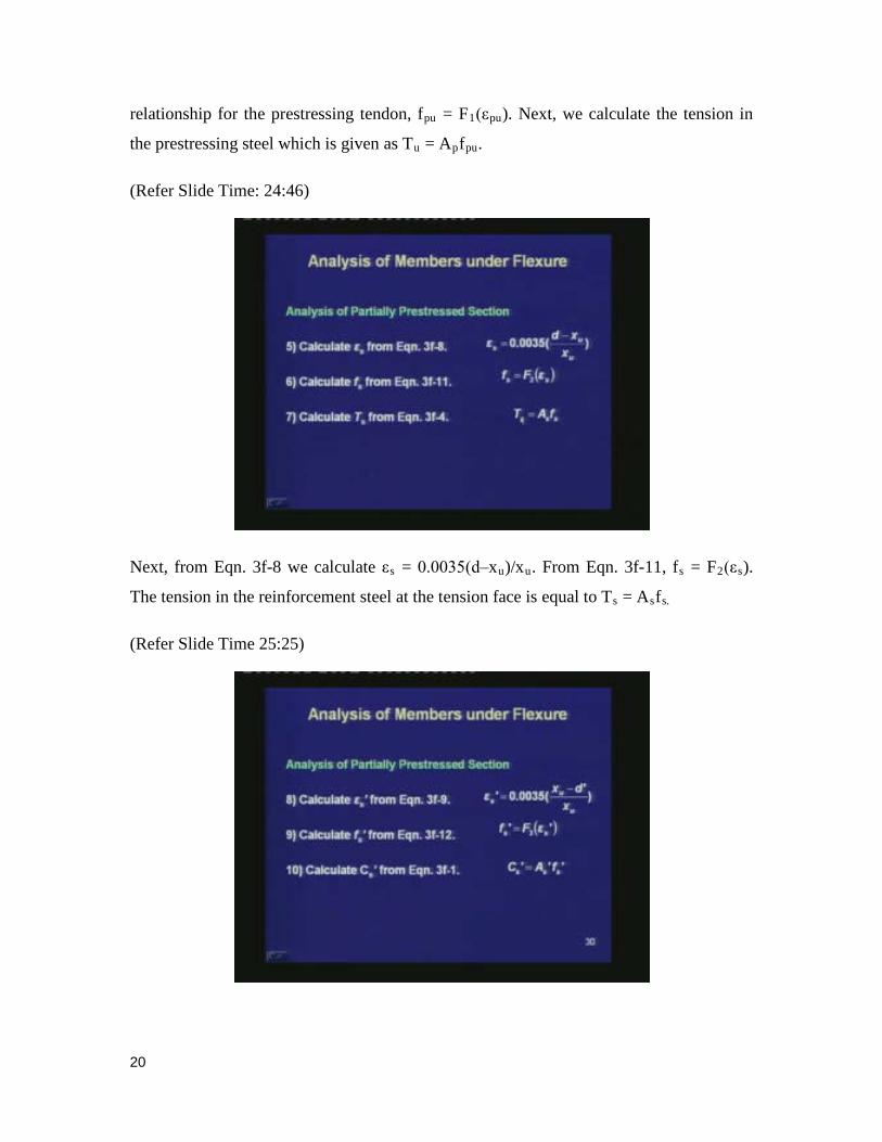
relationship for the prestressing tendon, fpu = F1(εpu). Next, we calculate the tension in
the prestressing steel which is given as Tu = Apfpu.
(Refer Slide Time: 24:46)
Next, from Eqn. 3f-8 we calculate εs = 0.0035(d‒xu)/xu. From Eqn. 3f-11, fs = F2(εs).
The tension in the reinforcement steel at the tension face is equal to Ts = Asfs.
(Refer Slide Time 25:25)
20
Finally, we calculate the strain in the steel close to the compression face. From Eqn. 3f-9,
εs/ = 0.0035(xu‒d/)/xu. From Eqn. 3f-12, fs
/ = F3(εs/). Next, Cs
/ = As/ fs
/.
(Refer Slide Time 26:01)
Thus, what we did till now is from the compatibility equations, we calculated the strain in
each layer of the steel. From the strain, we calculated the stress from the constitutive
relationship, and from the stress we calculated the force carried by each layer of steel.
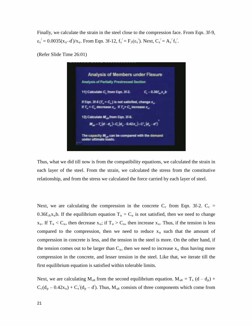
Next, we are calculating the compression in the concrete Cc from Eqn. 3f-2. Cc =
0.36fckxub. If the equilibrium equation Tu = Cu is not satisfied, then we need to change
xu. If Tu < Cu, then decrease xu; if Tu > Cu, then increase xu. Thus, if the tension is less
compared to the compression, then we need to reduce xu such that the amount of
compression in concrete is less, and the tension in the steel is more. On the other hand, if
the tension comes out to be larger than Cu, then we need to increase xu thus having more
compression in the concrete, and lesser tension in the steel. Like that, we iterate till the
first equilibrium equation is satisfied within tolerable limits.
Next, we are calculating MuR from the second equilibrium equation. MuR = Ts (d ‒ dp) +
Cc(dp ‒ 0.42xu) + Cs/(dp ‒ d/). Thus, MuR consists of three components which come from
21
the three forces multiplied by the respective lever arms with respect to the CGS. Once we
have calculated the capacity MuR, we compare it with the demand under the ultimate
loads.
Next we move on to the analysis of an unbonded post-tensioned beam.
(Refer Slide Time 28:40)
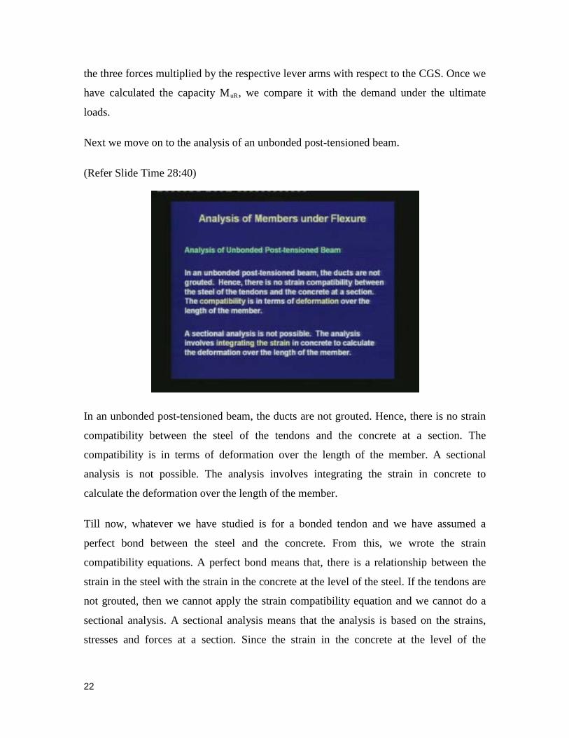
In an unbonded post-tensioned beam, the ducts are not grouted. Hence, there is no strain
compatibility between the steel of the tendons and the concrete at a section. The
compatibility is in terms of deformation over the length of the member. A sectional
analysis is not possible. The analysis involves integrating the strain in concrete to
calculate the deformation over the length of the member.
Till now, whatever we have studied is for a bonded tendon and we have assumed a
perfect bond between the steel and the concrete. From this, we wrote the strain
compatibility equations. A perfect bond means that, there is a relationship between the
strain in the steel with the strain in the concrete at the level of the steel. If the tendons are
not grouted, then we cannot apply the strain compatibility equation and we cannot do a
sectional analysis. A sectional analysis means that the analysis is based on the strains,
stresses and forces at a section. Since the strain in the concrete at the level of the
22
prestressing steel and the strain in the prestressing steel are not related by an equation
throughout the loading, we cannot use the conventional analysis for an unbonded tendon.
For an unbonded tendon, we write the compatibility equation in a different way. We write
the compatibility in terms of the total deformation of the concrete at the level of the
prestressing steel, and the deformation of the prestressing steel. Since we need to
calculate the deformation of the concrete throughout the length of the member, we need
to integrate the strain in the concrete at the level of prestressing steel.
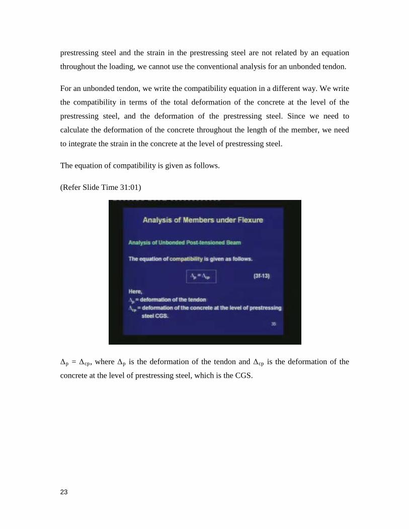
The equation of compatibility is given as follows.
(Refer Slide Time 31:01)
Δp = Δcp, where Δp is the deformation of the tendon and Δcp is the deformation of the
concrete at the level of prestressing steel, which is the CGS.
23
(Refer Slide Time: 31:21)
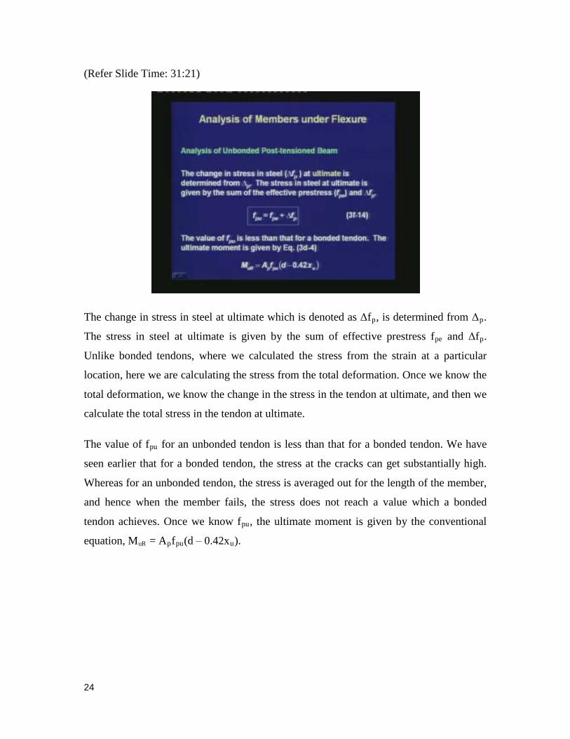
The change in stress in steel at ultimate which is denoted as Δfp, is determined from Δp.
The stress in steel at ultimate is given by the sum of effective prestress fpe and Δfp.
Unlike bonded tendons, where we calculated the stress from the strain at a particular
location, here we are calculating the stress from the total deformation. Once we know the
total deformation, we know the change in the stress in the tendon at ultimate, and then we
calculate the total stress in the tendon at ultimate.
The value of fpu for an unbonded tendon is less than that for a bonded tendon. We have
seen earlier that for a bonded tendon, the stress at the cracks can get substantially high.
Whereas for an unbonded tendon, the stress is averaged out for the length of the member,
and hence when the member fails, the stress does not reach a value which a bonded
tendon achieves. Once we know fpu, the ultimate moment is given by the conventional
equation, MuR = Apfpu(d ‒ 0.42xu).
24
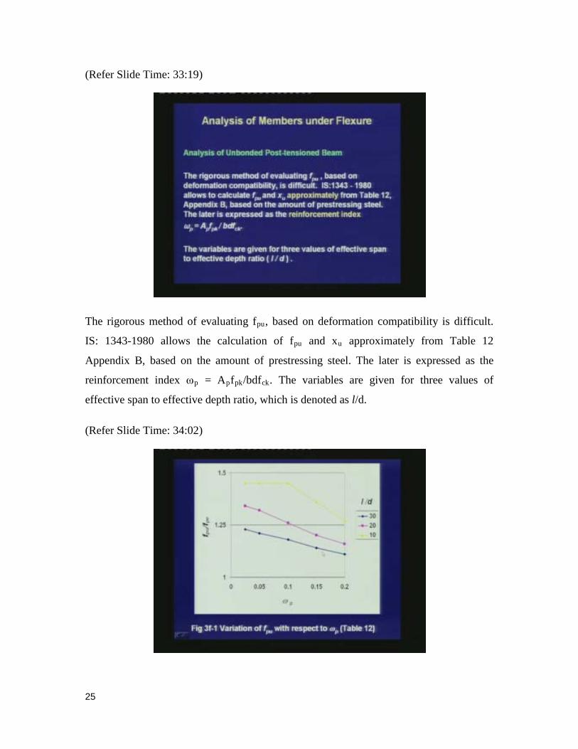
(Refer Slide Time: 33:19)
The rigorous method of evaluating fpu, based on deformation compatibility is difficult.
IS: 1343-1980 allows the calculation of fpu and xu approximately from Table 12
Appendix B, based on the amount of prestressing steel. The later is expressed as the
reinforcement index ωp = Apfpk/bdfck. The variables are given for three values of
effective span to effective depth ratio, which is denoted as l/d.
(Refer Slide Time: 34:02)
25
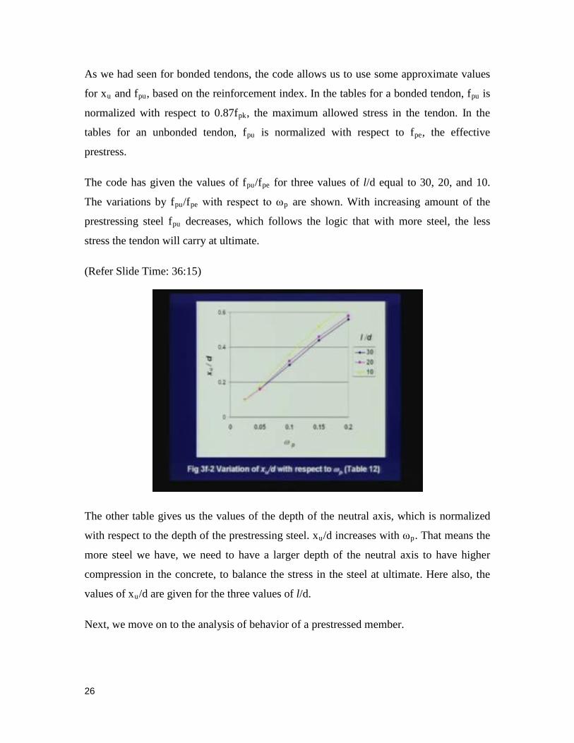
As we had seen for bonded tendons, the code allows us to use some approximate values
for xu and fpu, based on the reinforcement index. In the tables for a bonded tendon, fpu is
normalized with respect to 0.87fpk, the maximum allowed stress in the tendon. In the
tables for an unbonded tendon, fpu is normalized with respect to fpe, the effective
prestress.
The code has given the values of fpu/fpe for three values of l/d equal to 30, 20, and 10.
The variations by fpu/fpe with respect to ωp are shown. With increasing amount of the
prestressing steel fpu decreases, which follows the logic that with more steel, the less
stress the tendon will carry at ultimate.
(Refer Slide Time: 36:15)
The other table gives us the values of the depth of the neutral axis, which is normalized
with respect to the depth of the prestressing steel. xu/d increases with ωp. That means the
more steel we have, we need to have a larger depth of the neutral axis to have higher
compression in the concrete, to balance the stress in the steel at ultimate. Here also, the
values of xu/d are given for the three values of l/d.
Next, we move on to the analysis of behavior of a prestressed member.
26
(Refer Slide Time 36:54)
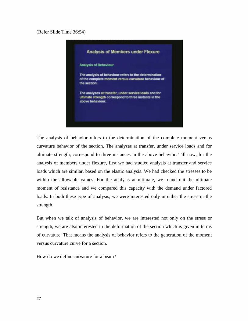
The analysis of behavior refers to the determination of the complete moment versus
curvature behavior of the section. The analyses at transfer, under service loads and for
ultimate strength, correspond to three instances in the above behavior. Till now, for the
analysis of members under flexure, first we had studied analysis at transfer and service
loads which are similar, based on the elastic analysis. We had checked the stresses to be
within the allowable values. For the analysis at ultimate, we found out the ultimate
moment of resistance and we compared this capacity with the demand under factored
loads. In both these type of analysis, we were interested only in either the stress or the
strength.
But when we talk of analysis of behavior, we are interested not only on the stress or
strength, we are also interested in the deformation of the section which is given in terms
of curvature. That means the analysis of behavior refers to the generation of the moment
versus curvature curve for a section.
How do we define curvature for a beam?
27
(Refer Slide Time: 38:44)
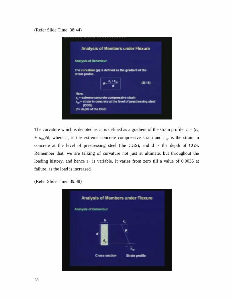
The curvature which is denoted as ϕ, is defined as a gradient of the strain profile. ϕ = (εc
+ εcp)/d, where εc is the extreme concrete compressive strain and εcp is the strain in
concrete at the level of prestressing steel (the CGS), and d is the depth of CGS.
Remember that, we are talking of curvature not just at ultimate, but throughout the
loading history, and hence εc is variable. It varies from zero till a value of 0.0035 at
failure, as the load is increased.
(Refer Slide Time: 39:38)
28
This sketch shows the definition of curvature which is equal to the gradient of the strain
profile.
(Refer Slide Time: 40:15)
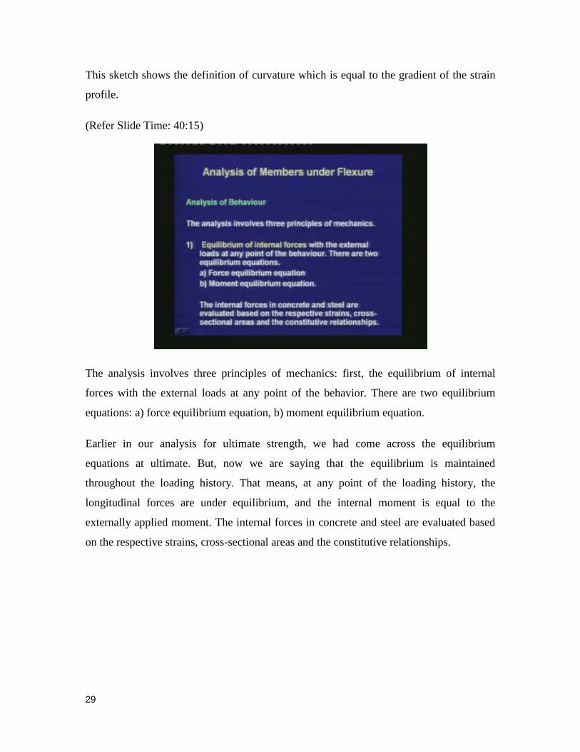
The analysis involves three principles of mechanics: first, the equilibrium of internal
forces with the external loads at any point of the behavior. There are two equilibrium
equations: a) force equilibrium equation, b) moment equilibrium equation.
Earlier in our analysis for ultimate strength, we had come across the equilibrium
equations at ultimate. But, now we are saying that the equilibrium is maintained
throughout the loading history. That means, at any point of the loading history, the
longitudinal forces are under equilibrium, and the internal moment is equal to the
externally applied moment. The internal forces in concrete and steel are evaluated based
on the respective strains, cross-sectional areas and the constitutive relationships.
29
(Refer Slide Time: 41:15)
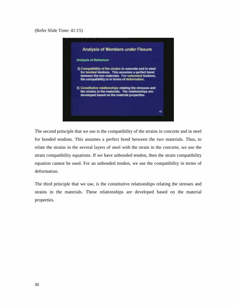
The second principle that we use is the compatibility of the strains in concrete and in steel
for bonded tendons. This assumes a perfect bond between the two materials. Thus, to
relate the strains in the several layers of steel with the strain in the concrete, we use the
strain compatibility equations. If we have unbonded tendon, then the strain compatibility
equation cannot be used. For an unbonded tendon, we use the compatibility in terms of
deformation.
The third principle that we use, is the constitutive relationships relating the stresses and
strains in the materials. These relationships are developed based on the material
properties.
30
(Refer Slide Time: 42:11)
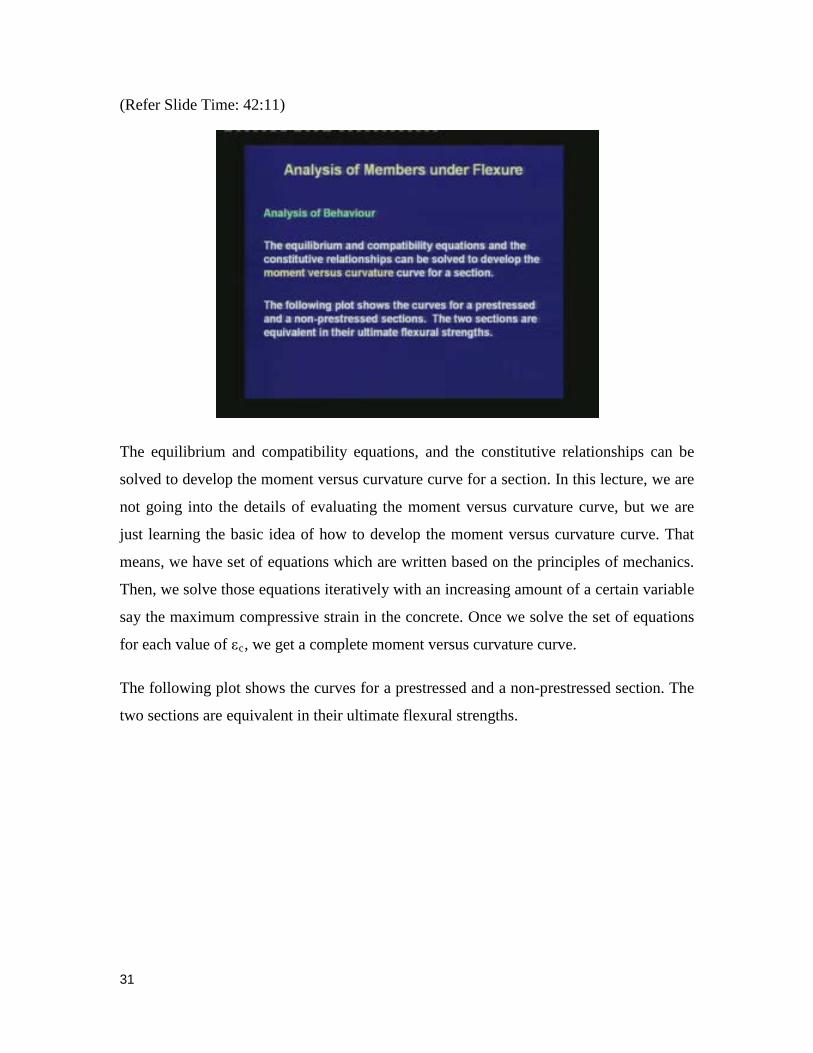
The equilibrium and compatibility equations, and the constitutive relationships can be
solved to develop the moment versus curvature curve for a section. In this lecture, we are
not going into the details of evaluating the moment versus curvature curve, but we are
just learning the basic idea of how to develop the moment versus curvature curve. That
means, we have set of equations which are written based on the principles of mechanics.
Then, we solve those equations iteratively with an increasing amount of a certain variable
say the maximum compressive strain in the concrete. Once we solve the set of equations
for each value of εc, we get a complete moment versus curvature curve.
The following plot shows the curves for a prestressed and a non-prestressed section. The
two sections are equivalent in their ultimate flexural strengths.
31
(Refer Slide Time: 43:21)
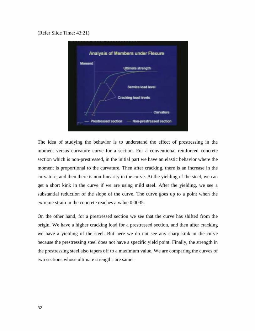
The idea of studying the behavior is to understand the effect of prestressing in the
moment versus curvature curve for a section. For a conventional reinforced concrete
section which is non-prestressed, in the initial part we have an elastic behavior where the
moment is proportional to the curvature. Then after cracking, there is an increase in the
curvature, and then there is non-linearity in the curve. At the yielding of the steel, we can
get a short kink in the curve if we are using mild steel. After the yielding, we see a
substantial reduction of the slope of the curve. The curve goes up to a point when the
extreme strain in the concrete reaches a value 0.0035.
On the other hand, for a prestressed section we see that the curve has shifted from the
origin. We have a higher cracking load for a prestressed section, and then after cracking
we have a yielding of the steel. But here we do not see any sharp kink in the curve
because the prestressing steel does not have a specific yield point. Finally, the strength in
the prestressing steel also tapers off to a maximum value. We are comparing the curves of
two sections whose ultimate strengths are same.
32
(Refer Slide Time: 45:21)
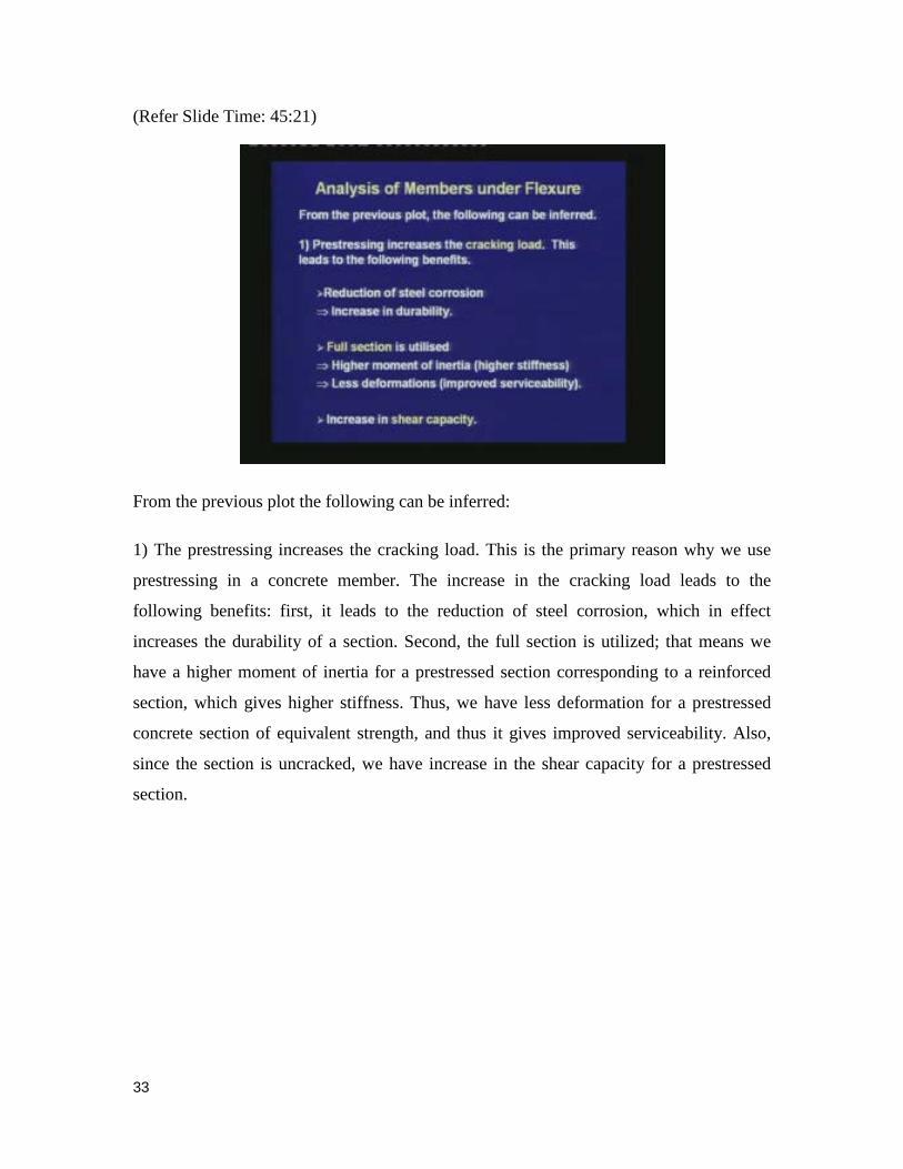
From the previous plot the following can be inferred:
1) The prestressing increases the cracking load. This is the primary reason why we use
prestressing in a concrete member. The increase in the cracking load leads to the
following benefits: first, it leads to the reduction of steel corrosion, which in effect
increases the durability of a section. Second, the full section is utilized; that means we
have a higher moment of inertia for a prestressed section corresponding to a reinforced
section, which gives higher stiffness. Thus, we have less deformation for a prestressed
concrete section of equivalent strength, and thus it gives improved serviceability. Also,
since the section is uncracked, we have increase in the shear capacity for a prestressed
section.
33
(Refer Slide Time: 46:33)
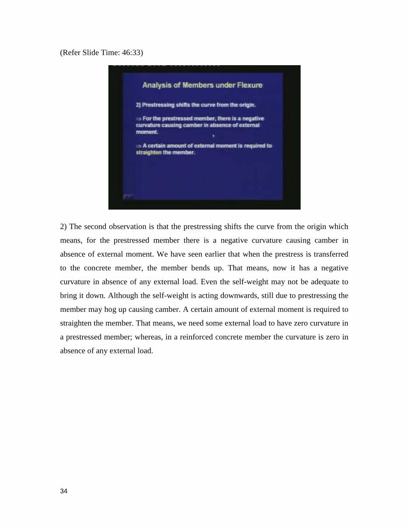
2) The second observation is that the prestressing shifts the curve from the origin which
means, for the prestressed member there is a negative curvature causing camber in
absence of external moment. We have seen earlier that when the prestress is transferred
to the concrete member, the member bends up. That means, now it has a negative
curvature in absence of any external load. Even the self-weight may not be adequate to
bring it down. Although the self-weight is acting downwards, still due to prestressing the
member may hog up causing camber. A certain amount of external moment is required to
straighten the member. That means, we need some external load to have zero curvature in
a prestressed member; whereas, in a reinforced concrete member the curvature is zero in
absence of any external load.
34
(Refer Slide Time: 47:50)
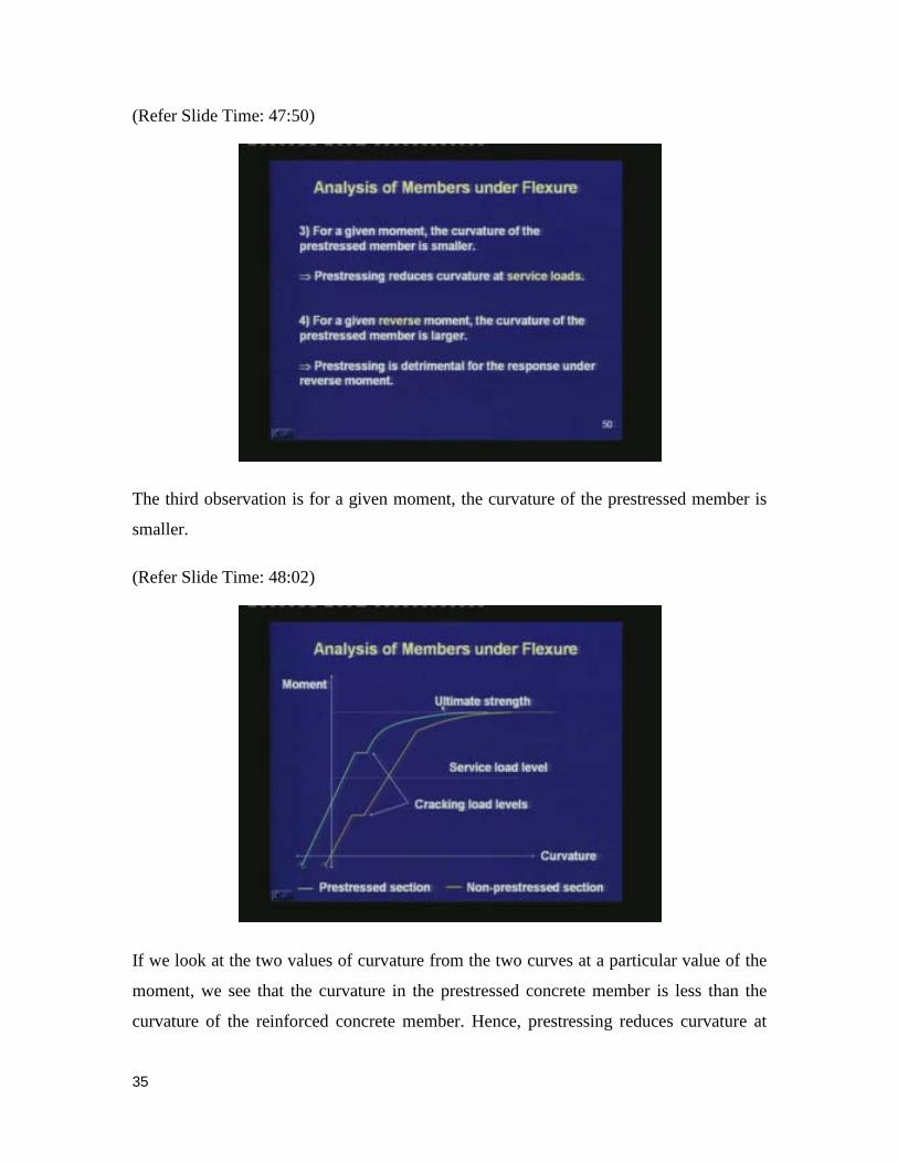
The third observation is for a given moment, the curvature of the prestressed member is
smaller.
(Refer Slide Time: 48:02)
If we look at the two values of curvature from the two curves at a particular value of the
moment, we see that the curvature in the prestressed concrete member is less than the
curvature of the reinforced concrete member. Hence, prestressing reduces curvature at
35
service loads which gives less deflection at service loads. The fourth inference is, for a
given reverse moment the curvature of the prestressed member is larger. In case if the
moment reverses, then the curvature of the prestressed concrete member will be higher
than that of a reinforced concrete section. We can conclude that prestressing is
detrimental for the response under reverse moment.
(Refer Slide Time: 49:03)
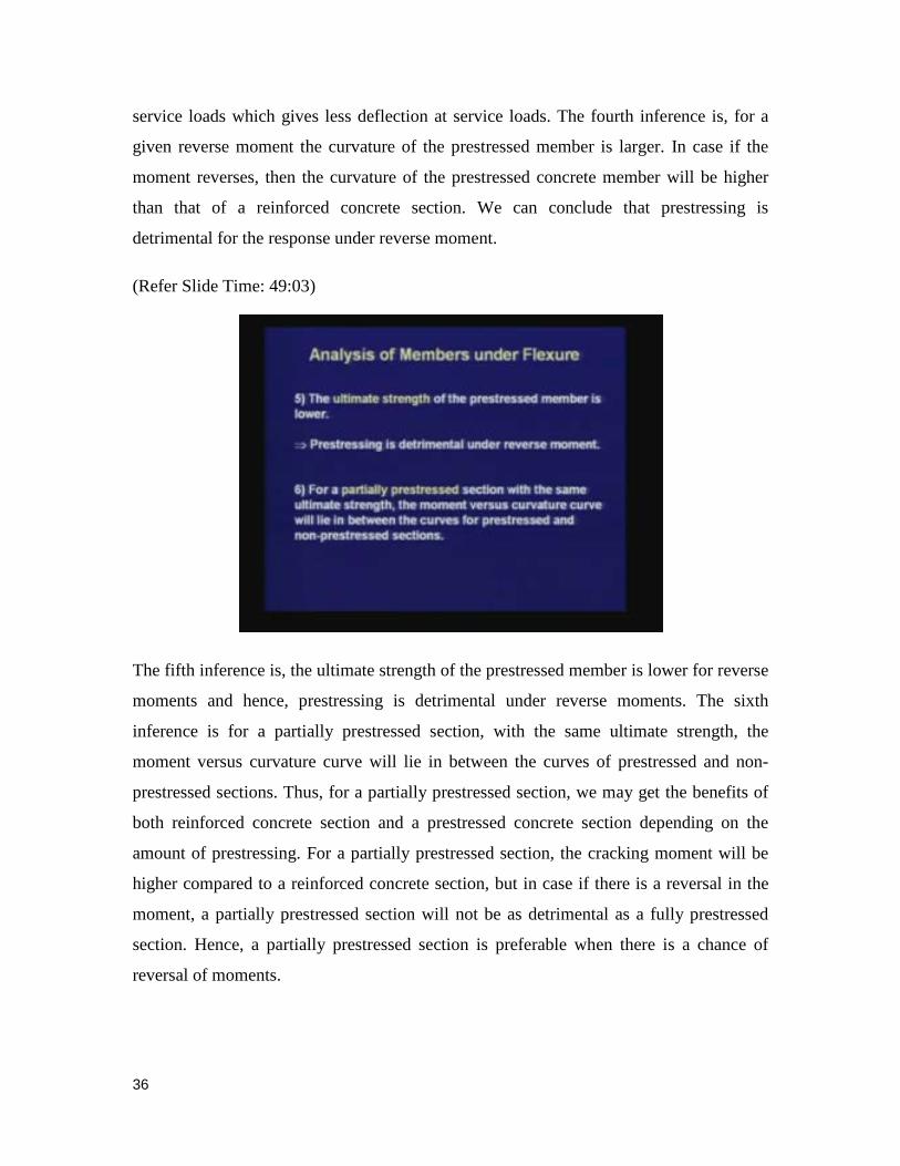
The fifth inference is, the ultimate strength of the prestressed member is lower for reverse
moments and hence, prestressing is detrimental under reverse moments. The sixth
inference is for a partially prestressed section, with the same ultimate strength, the
moment versus curvature curve will lie in between the curves of prestressed and non-
prestressed sections. Thus, for a partially prestressed section, we may get the benefits of
both reinforced concrete section and a prestressed concrete section depending on the
amount of prestressing. For a partially prestressed section, the cracking moment will be
higher compared to a reinforced concrete section, but in case if there is a reversal in the
moment, a partially prestressed section will not be as detrimental as a fully prestressed
section. Hence, a partially prestressed section is preferable when there is a chance of
reversal of moments.
36
Another important concept, we come to know by studying the behavior is the concept of
ductility. The ductility is the measure of energy absorption.
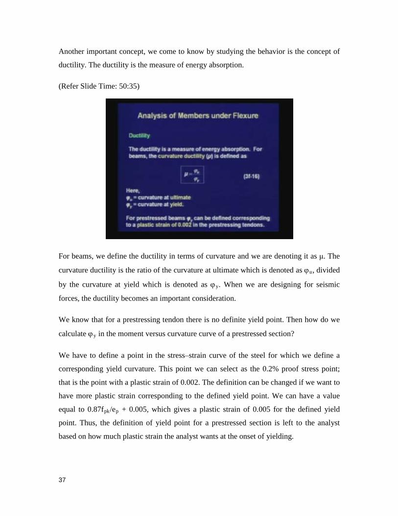
(Refer Slide Time: 50:35)
For beams, we define the ductility in terms of curvature and we are denoting it as μ. The
curvature ductility is the ratio of the curvature at ultimate which is denoted as ϕu, divided
by the curvature at yield which is denoted as ϕy. When we are designing for seismic
forces, the ductility becomes an important consideration.
We know that for a prestressing tendon there is no definite yield point. Then how do we
calculate ϕy in the moment versus curvature curve of a prestressed section?
We have to define a point in the stress‒strain curve of the steel for which we define a
corresponding yield curvature. This point we can select as the 0.2% proof stress point;
that is the point with a plastic strain of 0.002. The definition can be changed if we want to
have more plastic strain corresponding to the defined yield point. We can have a value
equal to 0.87fpk/ep + 0.005, which gives a plastic strain of 0.005 for the defined yield
point. Thus, the definition of yield point for a prestressed section is left to the analyst
based on how much plastic strain the analyst wants at the onset of yielding.
37
(Refer Slide Time 52:45)
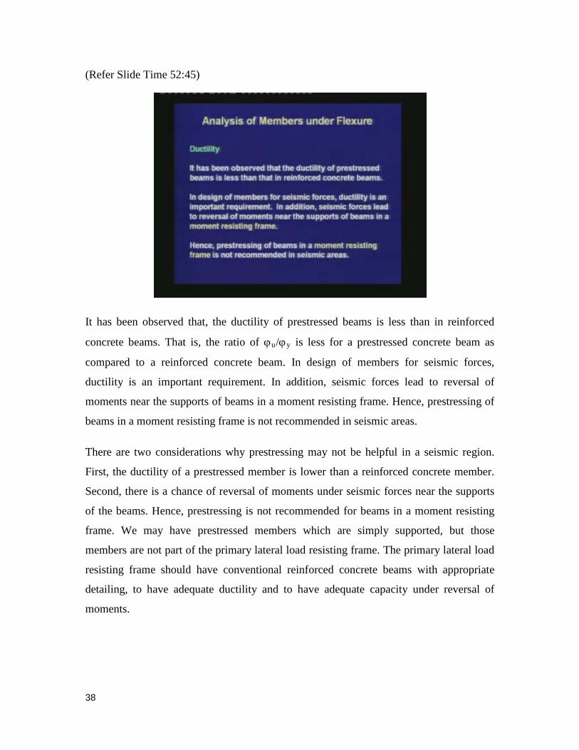
It has been observed that, the ductility of prestressed beams is less than in reinforced
concrete beams. That is, the ratio of ϕu/ϕy is less for a prestressed concrete beam as
compared to a reinforced concrete beam. In design of members for seismic forces,
ductility is an important requirement. In addition, seismic forces lead to reversal of
moments near the supports of beams in a moment resisting frame. Hence, prestressing of
beams in a moment resisting frame is not recommended in seismic areas.
There are two considerations why prestressing may not be helpful in a seismic region.
First, the ductility of a prestressed member is lower than a reinforced concrete member.
Second, there is a chance of reversal of moments under seismic forces near the supports
of the beams. Hence, prestressing is not recommended for beams in a moment resisting
frame. We may have prestressed members which are simply supported, but those
members are not part of the primary lateral load resisting frame. The primary lateral load
resisting frame should have conventional reinforced concrete beams with appropriate
detailing, to have adequate ductility and to have adequate capacity under reversal of
moments.
38
(Refer Slide Time: 54:30)
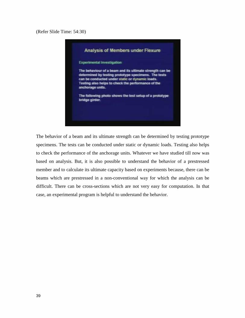
The behavior of a beam and its ultimate strength can be determined by testing prototype
specimens. The tests can be conducted under static or dynamic loads. Testing also helps
to check the performance of the anchorage units. Whatever we have studied till now was
based on analysis. But, it is also possible to understand the behavior of a prestressed
member and to calculate its ultimate capacity based on experiments because, there can be
beams which are prestressed in a non-conventional way for which the analysis can be
difficult. There can be cross-sections which are not very easy for computation. In that
case, an experimental program is helpful to understand the behavior.
39
(Refer Slide Time: 55:41)
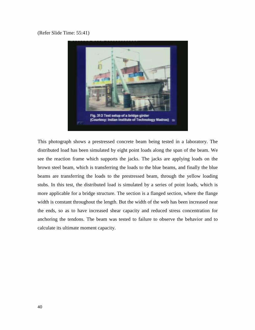
This photograph shows a prestressed concrete beam being tested in a laboratory. The
distributed load has been simulated by eight point loads along the span of the beam. We
see the reaction frame which supports the jacks. The jacks are applying loads on the
brown steel beam, which is transferring the loads to the blue beams, and finally the blue
beams are transferring the loads to the prestressed beam, through the yellow loading
stubs. In this test, the distributed load is simulated by a series of point loads, which is
more applicable for a bridge structure. The section is a flanged section, where the flange
width is constant throughout the length. But the width of the web has been increased near
the ends, so as to have increased shear capacity and reduced stress concentration for
anchoring the tendons. The beam was tested to failure to observe the behavior and to
calculate its ultimate moment capacity.
40
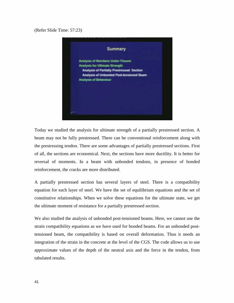
(Refer Slide Time: 57:23)
Today we studied the analysis for ultimate strength of a partially prestressed section. A
beam may not be fully prestressed. There can be conventional reinforcement along with
the prestressing tendon. There are some advantages of partially prestressed sections. First
of all, the sections are economical. Next, the sections have more ductility. It is better for
reversal of moments. In a beam with unbonded tendons, in presence of bonded
reinforcement, the cracks are more distributed.
A partially prestressed section has several layers of steel. There is a compatibility
equation for each layer of steel. We have the set of equilibrium equations and the set of
constitutive relationships. When we solve these equations for the ultimate state, we get
the ultimate moment of resistance for a partially prestressed section.
We also studied the analysis of unbonded post-tensioned beams. Here, we cannot use the
strain compatibility equations as we have used for bonded beams. For an unbonded post-
tensioned beam, the compatibility is based on overall deformation. Thus it needs an
integration of the strain in the concrete at the level of the CGS. The code allows us to use
approximate values of the depth of the neutral axis and the force in the tendon, from
tabulated results.
41
Finally, we studied the analysis of behavior, where we understood the moment versus
curvature curve for a prestressed section as compared to that for a reinforced concrete
section. We learned the concept of ductility. We understood the benefits and certain
drawbacks of prestressing. With this, we are ending the analysis of members. Next, we
shall move on to the design of prestressed concrete members.
Thank you.
42