lecture 21: point-based rendering - cornell university · 3 © kavita bala, computer science,...

1

Lecture 21: Point-based Rendering

Fall 2004Kavita Bala

Computer ScienceCornell University

© Kavita Bala, Computer Science, Cornell University

Announcements• In-class exam next week Nov 18th.

• Regrade requests in writing– Will regrade whole assignment


Complexity• Lighting: many lights, environment maps

– Global illumination, shadows

• Materials: BRDFs, textures

• Geometry: Level-of-detail, point-based representations

• All: impostors, image-based rendering


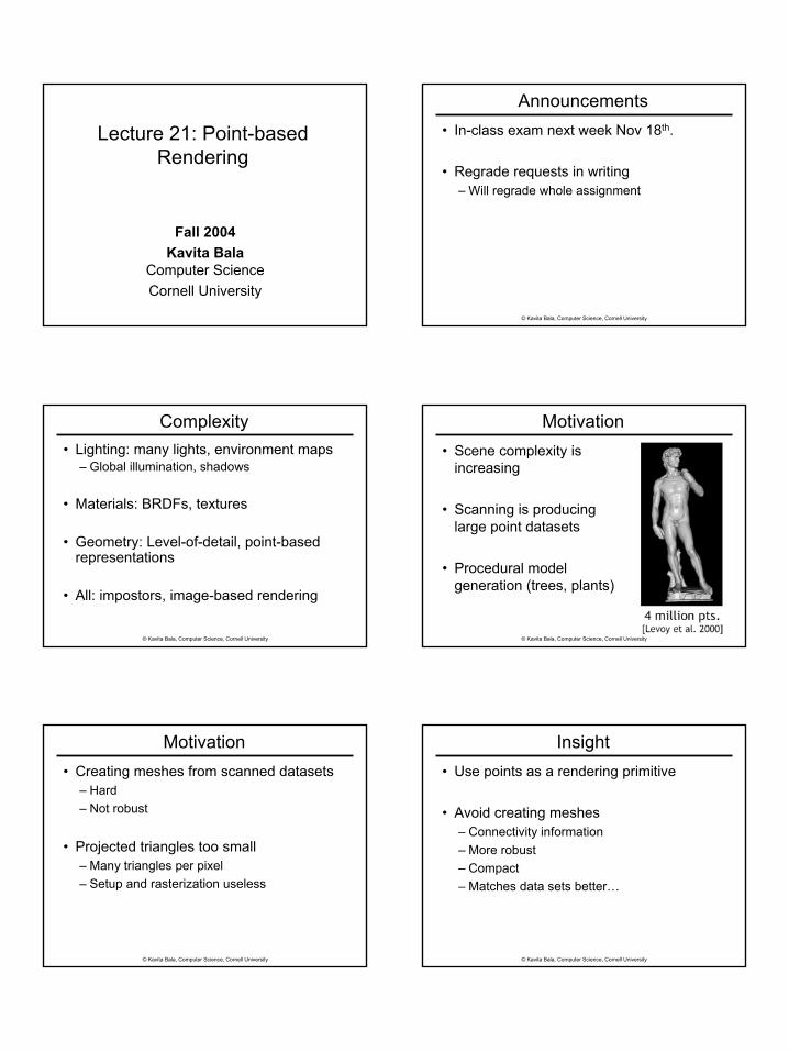
Motivation• Scene complexity is

increasing

• Scanning is producing large point datasets

• Procedural model generation (trees, plants)


Motivation• Creating meshes from scanned datasets

– Hard– Not robust

• Projected triangles too small– Many triangles per pixel– Setup and rasterization useless


Insight• Use points as a rendering primitive

• Avoid creating meshes– Connectivity information– More robust– Compact– Matches data sets better…

2


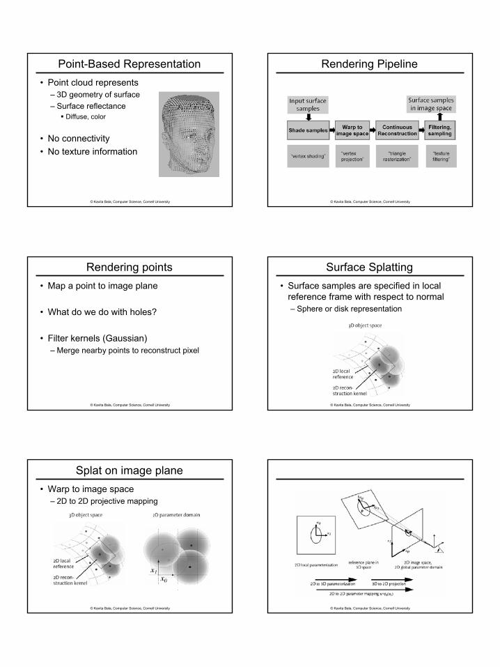
Point-Based Representation• Point cloud represents

– 3D geometry of surface– Surface reflectance

Diffuse, color

• No connectivity• No texture information


Rendering Pipeline


Rendering points• Map a point to image plane

• What do we do with holes?

• Filter kernels (Gaussian)– Merge nearby points to reconstruct pixel


Surface Splatting• Surface samples are specified in local

reference frame with respect to normal– Sphere or disk representation


Splat on image plane• Warp to image space

– 2D to 2D projective mapping


3


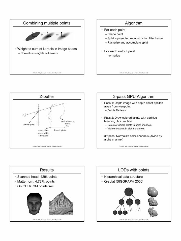
Combining multiple points

• Weighted sum of kernels in image space– Normalize weights of kernels


Algorithm• For each point

– Shade point– Splat = projected reconstruction filter kernel– Rasterize and accumulate splat

• For each output pixel– normalize


Z-buffer


3-pass GPU Algorithm• Pass 1: Depth image with depth offset epsilon

away from viewpoint– Do z-buffer tests

• Pass 2: Draw colored splats with additive blending. Accumulate– Colors of visible splats in color channels– Visible footprint in alpha channels

• 3rd pass: Normalize color channels (divide by alpha channel)


Results• Scanned head: 429k points• Matterhorn: 4,787k points• On GPUs: 3M points/sec


LODs with points• Hierarchical data structure• Q-splat [SIGGRAPH 2000]

4


Construction• Each vertex of original mesh is leaf sphere

(such that adjacent vertices overlap)

• Construct top down

• Store sphere center, radius, normal– All quantized for compactness


Hierarchical Traversal

© Kavita Bala, Computer Science, Cornell University © Kavita Bala, Computer Science, Cornell University


Results

130k splats, 132 ms 1M splats, 722 ms


Other point-based work• Anti-aliasing of points/textures

• Hybrid rendering: polygons and points

• Point editing and animation

• Expensive shading with points: open question

5


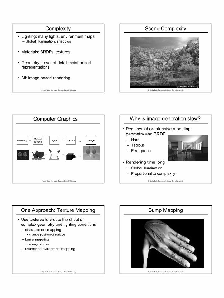
Complexity• Lighting: many lights, environment maps

– Global illumination, shadows

• Materials: BRDFs, textures

• Geometry: Level-of-detail, point-based representations

• All: image-based rendering


Scene Complexity


+

+

=

=

Computer Graphics

Geometry Camera ImageMaterial(BRDF) Lights+

+

+

+


Why is image generation slow?

• Requires labor-intensive modeling: geometry and BRDF – Hard– Tedious– Error-prone

• Rendering time long– Global illumination– Proportional to complexity


One Approach: Texture Mapping

• Use textures to create the effect of complex geometry and lighting conditions– displacement mapping

change position of surface– bump mapping

change normal– reflection/environment mapping


Bump Mapping

6


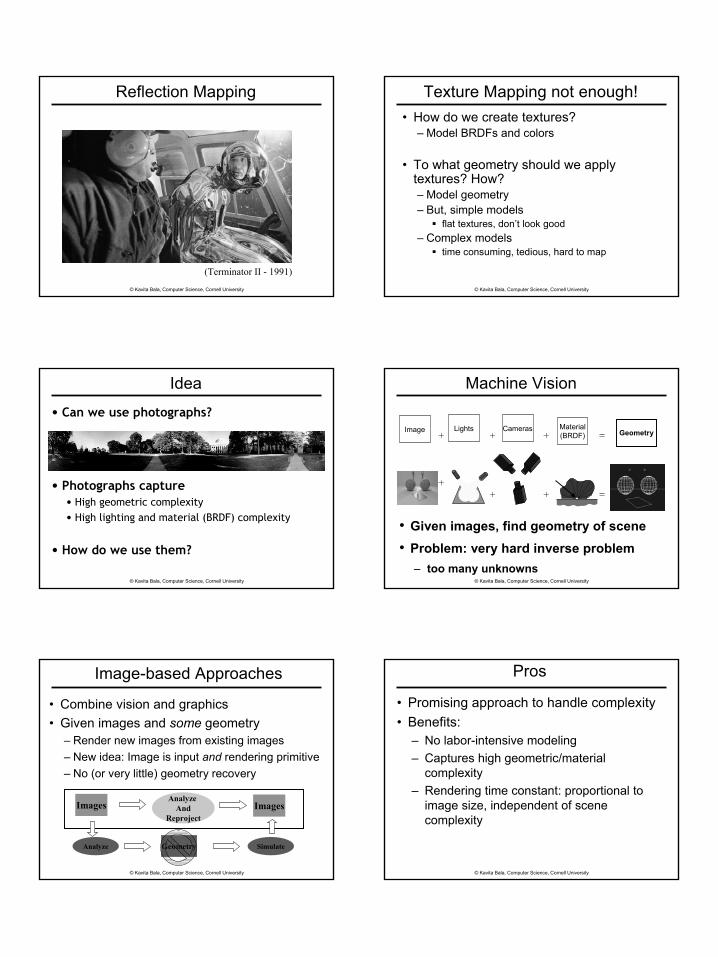
Reflection Mapping

(Terminator II - 1991)


Texture Mapping not enough!• How do we create textures?

– Model BRDFs and colors

• To what geometry should we apply textures? How?– Model geometry– But, simple models

flat textures, don’t look good– Complex models

time consuming, tedious, hard to map


Idea

• Can we use photographs?

• Photographs capture• High geometric complexity• High lighting and material (BRDF) complexity

• How do we use them?


GeometryCameras+

+

=

=

Machine Vision

Lights+

+

+

+

• Given images, find geometry of scene• Problem: very hard inverse problem

– too many unknowns

Image Material(BRDF)


Image-based Approaches

• Combine vision and graphics • Given images and some geometry

– Render new images from existing images– New idea: Image is input and rendering primitive– No (or very little) geometry recovery

Images ImagesAnalyze

AndReproject

Analyze Geometry Simulate


Pros

• Promising approach to handle complexity• Benefits:

– No labor-intensive modeling– Captures high geometric/material

complexity– Rendering time constant: proportional to

image size, independent of scene complexity

7


Outline

• Theory

• Image-based Rendering

• Image-based Modeling– Façade


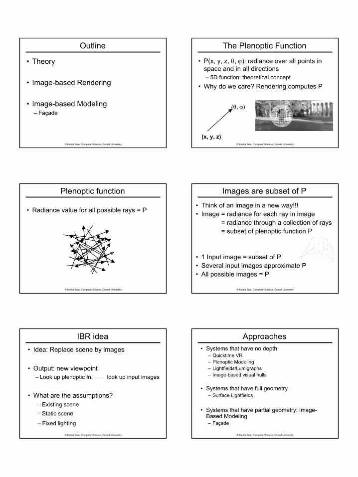
The Plenoptic Function

• P(x, y, z, θ, ϕ): radiance over all points in space and in all directions– 5D function: theoretical concept

• Why do we care? Rendering computes P

(x, y, z)

(θ, ϕ)


Plenoptic function

• Radiance value for all possible rays = P


Images are subset of P

• Think of an image in a new way!!!• Image = radiance for each ray in image

= radiance through a collection of rays= subset of plenoptic function P

• 1 Input image = subset of P • Several input images approximate P• All possible images = P


IBR idea• Idea: Replace scene by images

• Output: new viewpoint– Look up plenoptic fn. look up input images

• What are the assumptions?

– Static scene

– Fixed lighting

– Existing scene


Approaches• Systems that have no depth

– Quicktime VR– Plenoptic Modeling– Lightfields/Lumigraphs– Image-based visual hulls

• Systems that have full geometry– Surface Lightfields

• Systems that have partial geometry: Image-Based Modeling– Façade

8


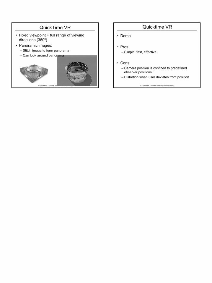
QuickTime VR• Fixed viewpoint + full range of viewing

directions (3600)• Panoramic images:

– Stitch image to form panorama– Can look around panorama


Quicktime VR

• Demo

• Pros– Simple, fast, effective

• Cons– Camera position is confined to predefined

observer positions– Distortion when user deviates from position

lecture 21: point-based rendering - cornell university · 3 © kavita bala, computer science,...

Documents