Lecture 26 1

Nodal Analysis

Lecture 26 2

Example: A Summing Circuit

• The output voltage V of this circuit is proportional to the sum of the two input currents I1 and I2.

• This circuit could be useful in audio applications or in instrumentation.

• The output of this circuit would probably be connected to an amplifier.

Lecture 26 3

+

-

V 500

500

1k

500

500I1 I2

Summing Circuit

V = 167I1 + 167I2

Lecture 26 4

Can you analyze this circuit using the techniques of Chapter

2?

Lecture 26 5

Not This One!

• There are no series or parallel resistors to combine.

• We do not have a single loop or a double node circuit.

• We need a more powerful analysis technique:

Nodal Analysis

Lecture 26 6

Why Nodal or Loop Analysis?

• The analysis techniques in Chapter 2 (voltage divider, equivalent resistance, etc.) provide an intuitive approach to analyzing circuits.

• They cannot analyze all circuits

• They cannot be easily automated by a computer.

Lecture 26 7

Node and Loop Analysis

• Node analysis and loop analysis are both circuit analysis methods which are systematic and apply to most circuits.

• Analysis of circuits using node or loop analysis requires solutions of systems of linear equations.

• These equations can usually be written by inspection of the circuit.

Lecture 26 8

Steps of Nodal Analysis

1. Choose a reference node.

2. Assign node voltages to the other nodes.

3. Apply KCL to each node other than the reference-express currents in terms of node voltages.

4. Solve the resulting system of linear equations.

Lecture 26 9

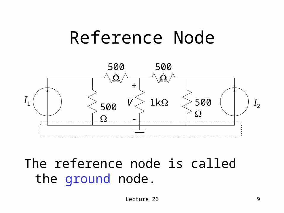
Reference Node

The reference node is called the ground node.

+

-

V 500

500

1k

500

500I1 I2

Lecture 26 10

Steps of Nodal Analysis

1. Choose a reference node.

2. Assign node voltages to the other nodes.

3. Apply KCL to each node other than the reference-express currents in terms of node voltages.

4. Solve the resulting system of linear equations.

Lecture 26 11

Node Voltages

V1, V2, and V3 are unknowns for which we solve using KCL.

500

500

1k

500

500I1 I2

1 2 3

V1 V2 V3

Lecture 26 12

Steps of Nodal Analysis

1. Choose a reference node.

2. Assign node voltages to the other nodes.

3. Apply KCL to each node other than the reference-express currents in terms of node voltages.

4. Solve the resulting system of linear equations.

Lecture 26 13

Currents and Node Voltages

500

V1500V1 V2

50021 VV

5001V

Lecture 26 14

KCL at Node 1

500

500I1

V1 V2

0500500

1211

VVV

I

Lecture 26 15

KCL at Node 2

500

1k

500 V2 V3V1

0500k1500

32212

VVVVV

Lecture 26 16

KCL at Node 3

500

500

I2

V2 V3

0500500 2

323

I

VVV

Lecture 26 17

Steps of Nodal Analysis

1. Choose a reference node.

2. Assign node voltages to the other nodes.

3. Apply KCL to each node other than the reference-express currents in terms of node voltages.

4. Solve the resulting system of linear equations.

Lecture 26 18

System of Equations

• Node 1:

• Node 2:

12

1 500500

1

500

1I

VV

0500500

1

k1

1

500

1

5003

21

VV

V

Lecture 26 19

System of Equations

• Node 3:

232

500

1

500

1

500IV

V

Lecture 26 20

Equations

• These equations can be written by inspection-the left side:

– The node voltage is multiplied by the sum of conductances of all resistors connected to the node.

– Other node voltages are multiplied by the conductance of the resistor(s) connecting to the node and subtracted.

Lecture 26 21

Equations

• The right side of the equation:

– The right side of the equation is the sum of currents from sources entering the node.

Lecture 26 22

Matrix Notation

• The three equations can be combined into a single matrix/vector equation.

2

1

3

2

1

0

500

1

500

1

500

10

500

1

500

1

k1

1

500

1

500

1

0500

1

500

1

500

1

I

I

V

V

V

Lecture 26 23

Matrix Notation

• The equation can be written in matrix-vector form as

Av = i

• The solution to the equation can be written as

v = A-1 i

Lecture 26 24

Solving the Equation with MATLAB

I1 = 3mA, I2 = 4mA

>> A = [1/500+1/500 -1/500 0;

-1/500 1/500+1/1000+1/500 -1/500;

0 -1/500 1/500+1/500];

>> i = [3e-3; 0; 4e-3];

Lecture 26 25

Solving the Equation

>> v = inv(A)*i

v =

1.3333

1.1667

1.5833

V1 = 1.33V, V2=1.17V, V3=1.58V