lecture 8: solving linear rationallinear rational

Lecture 8:Solving Linear RationalSolving Linear Rational Expectations Models

BU macro 2008 lecture 8 1

Five ComponentsFive Components

• A Core IdeasA. Core Ideas• B. Nonsingular Systems Theory

(Bl h d K h )– (Blanchard-Kahn)• C. Singular Systems Theory

– (King-Watson)• D. A Singular Systems Exampleg y p• E. Computation


A Core IdeasA. Core Ideas1. Recursive Forward Solution2. Law of Iterated Expectations3. Restrictions on Forcing Processesg4. Limiting Conditions5. Fundamental v. nonfundamental solutions6. Stable v. unstable roots7. Predetermined v. nonpredetermined variables8. Sargent’s procedure: unwind unstable roots

forward


Basic ExampleBasic Example

• Stock price as discounted sum of expectedStock price as discounted sum of expected future dividends

• Let pt be the (ex dividend) stock price and dt be pt ( ) p tdividends per share.

• Basic approach to stock valuationpp

1

11

jt t t j

j

p E d withr

β β∞

+=

= =+∑

• Intuitive reference model, although sometimes criticized for details and in applications

1j=


pp

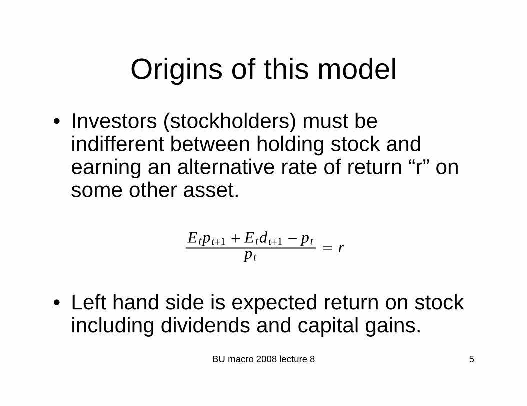
Origins of this modelOrigins of this model

• Investors (stockholders) must beInvestors (stockholders) must be indifferent between holding stock and earning an alternative rate of return “r” on gsome other asset.

Etpt1 Etdt1 − ptpt

r

• Left hand side is expected return on stock including dividends and capital gains.


including dividends and capital gains.

Rewriting this as an i l diff iexpectational difference equation

• Takes first order formTakes first order form

1 0 1 1General: a Et t t t t ty by c x c E x+ += + +1 0 1 1

1 1

Specific: (1 )t t t t t t

t t t t t

y y

E p r p E d+ +

+ += + −

• Alternatively

pt 11 r Etpt1 Etdt1


1 Recursive Forward Solution1. Recursive Forward Solution

• The process is straightforward but tediousThe process is straightforward but tedious,

pt Etp 1 d 1pt Etpt1 dt1

EtEt1pt2 dt2 dt1

. . .

∑J

jEtdtj JEtptJ∑j1


2 Law of Iterated Expectations2. Law of Iterated Expectations

• General result on conditional expectationsGeneral result on conditional expectations

EtEt1Et2 . .Etj−1x tj Etx tj

• Works in RE models where market

j j j

expectations are treated as conditional expectations

• Lets us move to last line above.


3. Restrictions on F i PForcing Processes

• One issue in moving to infinite horizon:One issue in moving to infinite horizon: first part of price (the sum) above is well defined so long as dividends don’t growdefined so long as dividends don t grow too fast, i.e.,

1jt t j tE d h withγ βγ+ ≤ <

• Under this condition,

liJ

jE d hβγ

β ≤∑BU macro 2008 lecture 8 91

lim1

jt t j t

J j

E d hβγ

ββγ+

→∞ =≤ < ∞

−∑

4 Limiting conditions4. Limiting conditions

• For the stock price to match the basic prediction,For the stock price to match the basic prediction, the second term must be zero in limit.

• For a finite stock price, there must be some limitp ,• The conventional assumption is that

• This is sometimes an implication (value of stock

lim 0JJ t t JE pβ→∞ + =

• This is sometimes an implication (value of stock must be bounded at any point in time would do it, for example).


, p )

5. Fundamental v. f d l l inonfundamental solutions

• Nonfundamental solutions are sometimesNonfundamental solutions are sometimes called bubble solutions.

• In the current setting let’s consider adding• In the current setting, let s consider adding an arbitrary sequence of random variables to the above: p f bto the above:

• These must be restricted by agents illi t h ld t k

pt f t bt

willingness to hold stock.

bt 1 Etbt1


bt 1 r Etbt1

Form of nonfundamental solutionsForm of nonfundamental solutions

• Stochastic difference equationStochastic difference equation

B bbl l ti i t d t l d t1 1 1(1 ) (1 )t t t t t tE b r b b r b ξ+ + += + ⇒ = + +

• Bubble solution is expected to explode at just the right rate,

so that it is not possible to eliminate the Etjbtj bt

plast term in the above.


Comments on BubblesComments on Bubbles

• A bursting bubble is one where there is aA bursting bubble is one where there is a big decline due to a particular random eventevent.

• Bubbles can’t be expected to burst (or they wouldn’t take place)they wouldn t take place)

• Bursting bubbles are hard to distinguish i i ll f ti i t d i iempirically from anticipated increases in

dividends that don’t materialize.


Ruling out bubbles of this formRuling out bubbles of this form

• Formal argumentsFormal arguments– Transversality condition

Informal procedures• Informal procedures– Unwind unstable roots forward (Sargent, see

below)below)– Sometimes motivated by type of data that one

seeks to explain (nonexplosive data)seeks to explain (nonexplosive data)


6. Unstable and Stable Roots i RE d lin RE models

• Stock price difference equation hasStock price difference equation has unstable root

• Write as• Write as

Etpt1 1 rpt Etdt1

• Root is (1+r)>1 if r>0.

p p

( )


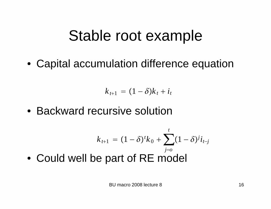
Stable root exampleStable root example

• Capital accumulation difference equationCapital accumulation difference equation

k 1 1 k i

• Backward recursive solution

k t1 1 − k t it

k t1 1 − tk 0 ∑t

1 − jit−j

• Could well be part of RE model

∑jo

j


7. Predetermined v. d i d i blnonpredetermined variables

• Stock price: nonpredetermined• Capital: predetermined• General solution practice so far captures

approach in literature

Predetermined NonPredetermined

Stable CapitalStable Capital

Unstable Stock Price


8 Sargent’s procedure8. Sargent s procedure

• In several contexts in the early 70sIn several contexts in the early 70s, Sargent made the suggestion that “unstable roots should be unwoundunstable roots should be unwound forward.”

• Examples:• Examples:– Money and prices: similar to stocks

L b d d ill t d thi l t– Labor demand: we will study this later.


B. Linear Difference Systems d R i l E iunder Rational Expectations

• Blanchard-Kahn: key contribution in the literature on how to solve RE macroeconomic models with a mixture of predeterminedRE macroeconomic models with a mixture of predetermined variables and nonpredetermined ones.

• Variant of their framework that we will study

EtYt1 WYt 0Xt 1EtXt1

• Y is column vector of endogenous variables, X is column vector of exgenous variables

EtYt1 WYt 0Xt 1EtXt1

exgenous variables• Other elements are fixed matrices (I,W, Ψ) that are conformable

with vectors (e.g. W is n(Y) by n(Y))


Types of VariablesTypes of Variables

• Predetermined (k): no response to xt-Et 1xtPredetermined (k): no response to xt Et-1xt

• Nonpredetermined (λ)• Endogenous variable vector is partitioned asEndogenous variable vector is partitioned as

Yt t

• Notation n(k) is number of k’s etc if we need to

Ytk t

• Notation n(k) is number of k s etc. if we need to be specific about it.


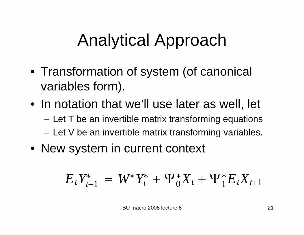
Analytical ApproachAnalytical Approach

• Transformation of system (of canonicalTransformation of system (of canonical variables form).

• In notation that we’ll use later as well let• In notation that we ll use later as well, let– Let T be an invertible matrix transforming equations

Let V be an invertible matrix transforming variables– Let V be an invertible matrix transforming variables.

• New system in current context

EtYt1∗ W∗Yt

∗ 0∗Xt 1

∗EtXt1


Transformed system of interestTransformed system of interest• Can be based on eigenvectors: WP=Pμg μ• T=inv(P) and V=inv(P)• Then we have

1 0 1 1

1 1 1 1 1

t t t t t tEY WY X E X

P EY P WPP Y P X P E X

+ +

− − − − −

= + Ψ + Ψ

+ Ψ + Ψ1 1 1 1 11 0 1 1

1 0 1 1

t t t t t t

t t t t t t

P EY P WPP Y P X P E X

EY JY X E X

+ +

∗ ∗ ∗ ∗+ +

= + Ψ + Ψ

= + Ψ + Ψ

with J block diagonal 0

0

u

s

JJ

J

⎡ ⎤⎢ ⎥= ⎢ ⎥⎢ ⎥⎣ ⎦


0 sJ⎢ ⎥⎣ ⎦

Jordan form matricesJordan form matrices

• Upper (or lower) diagonalUpper (or lower) diagonal• Repeated root “blocks” may have ones as

well as zeros above diagonalwell as zeros above diagonal.• Have inverses that are Jordan matrices

lalso.• Have zero limits if eigenvalues are all

stable


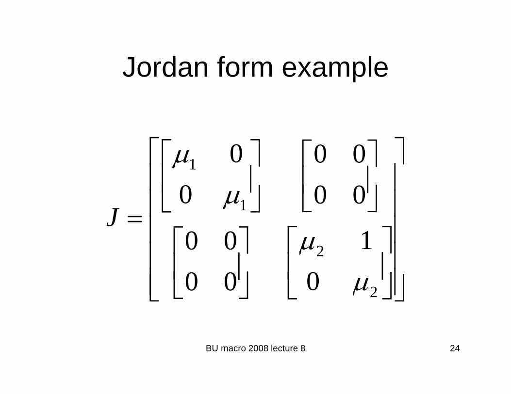
Jordan form exampleJordan form example

1 0 0 0μ⎡ ⎤⎡ ⎤ ⎡ ⎤⎢ ⎥⎢ ⎥ ⎢ ⎥

10 0 0J

μ⎢ ⎥⎢ ⎥ ⎢ ⎥⎣ ⎦⎣ ⎦⎢ ⎥= ⎢ ⎥

2 10 0J

μ= ⎢ ⎥⎡ ⎤⎡ ⎤⎢ ⎥⎢ ⎥⎢ ⎥⎢ ⎥⎣ ⎦ 200 0 μ⎢ ⎥⎢ ⎥⎢ ⎥⎣ ⎦ ⎣ ⎦⎣ ⎦


DiscussionDiscussion

• Jordan blocks:Jordan blocks: matrices containing common eigenvalues. 1 11: t t tB y y xμ −= +

• Form of Jordan block depends on structure of difference equation

1 1t t tz z xμ −= +

of difference equation (or canonical variables) 1 12 : t t tB y y zμ −= +

• Two examples shown at right

1 1t t tz z xμ −= +


Applying Sargent’s suggestionApplying Sargent s suggestion

• System is decoupled into equationsSystem is decoupled into equations describing variables with stable dynamics (s) and unstable dynamics (u)(s) and unstable dynamics (u)

• Taking the u part (with similarly partitioned matrices on x’s)matrices on x s)

Etut1 Juut 0u∗ Xt 1u

∗ EtXt1

• We can think about unwinding it forward.

t 0u 1u t


g

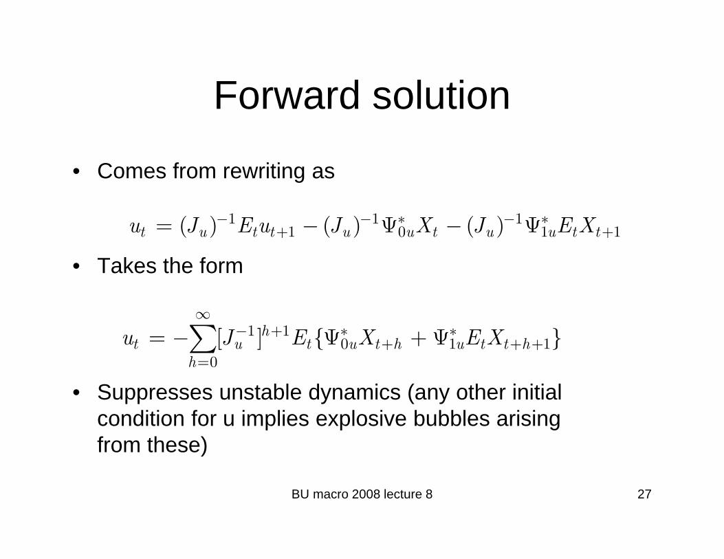
Forward solutionForward solution

• Comes from rewriting asComes from rewriting as

1 1 11 0 1 1( ) ( ) ( )t u t t u u t u u t tu J E u J X J E X− − ∗ − ∗

+ += − Ψ − Ψ

• Takes the form

∞

S t bl d i ( th i iti l

1 10 1 1

0

[ ] { }ht u t u t h u t t h

h

u J E X E X∞

− + ∗ ∗+ + +

== − Ψ + Ψ∑

• Suppresses unstable dynamics (any other initial condition for u implies explosive bubbles arising from these)


)

Stable block evolves according toStable block evolves according to

• The difference systemThe difference system

Etst1 Jsst C0s∗ Xt C1s

∗ EtXt1t t1 s t 0s t 1s t t1


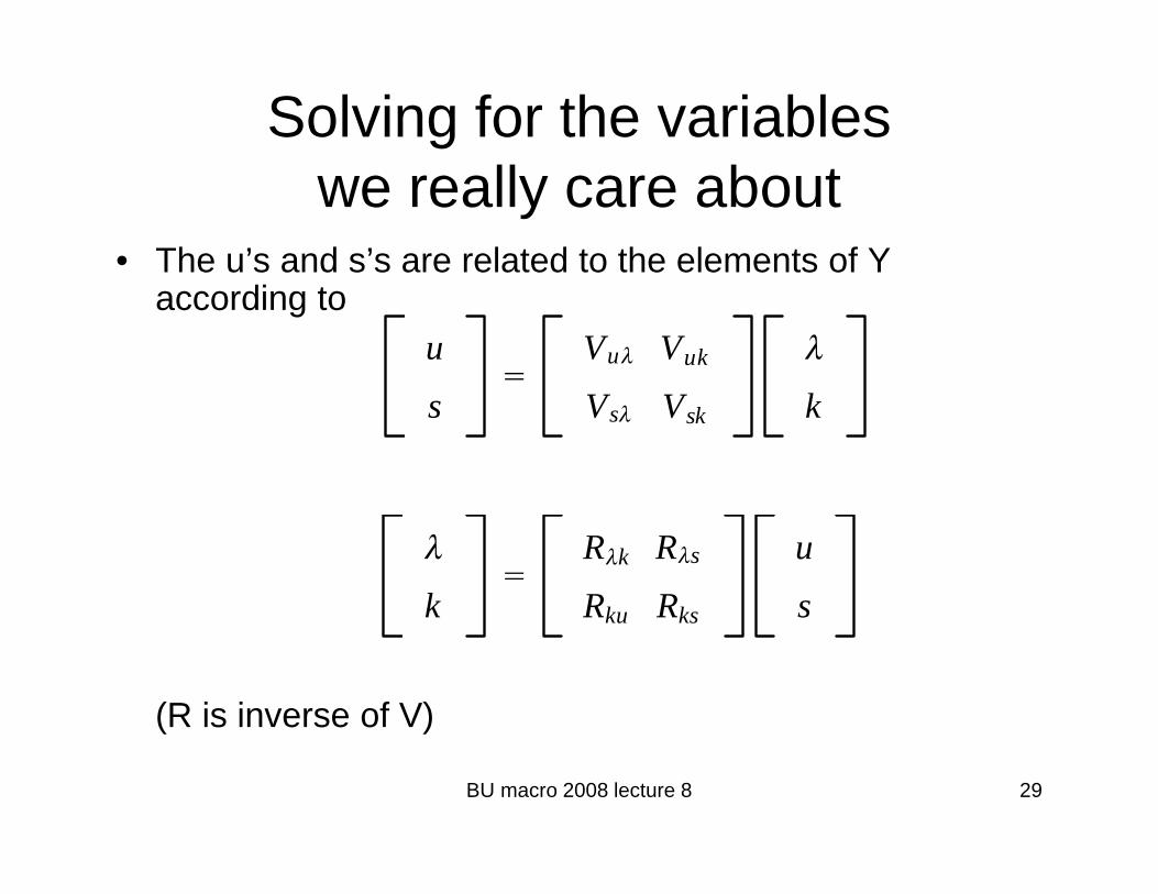
Solving for the variables ll bwe really care about

• The u’s and s’s are related to the elements of Y according to

u

Vu Vuk

s Vs Vsk k

k

Rk Rs

Rku Rks

u

s

(R is inverse of V)

k Rku Rks s


( )

Solving ford i d i blnonpredetermined variables

• Star Trek and Related MattersStar Trek and Related Matters• First “line” of matrix equation above

ut Vu t Vukk t.

• Solvable if we have two conditions– Same number of unstable andSame number of unstable and

nonpredetermined variables– Invertible matrix Vuλ


uλ

SolvingSolving

• We get nonpredetermined variables asWe get nonpredetermined variables as

1

1 1 10 1 1

[ ]

[ ] { }

t u t uk t

ht t h t t h

V u V k

V J E X E X

λ

λ

λ −

∞− − + ∗ ∗

+ + +

= −

= − Ψ + Ψ∑ 0 1 10

1

[ ] { }u u t u t h u t t hh

u uk t

V J E X E X

V V k

λ

λ

+ + +=

−

= Ψ + Ψ

−

∑


SolvingSolving

• We get the predetermined variables asWe get the predetermined variables as

k 1 wkkk wk 0kx 1kE x 1k t1 wkkk t wk t 0kx t 1kEtx t1

• (Apparently, somewhat different solutions arise if you use other equations to get future k’s but these are not

ll diff t)really different)


BK provideBK provide

• A tight description of how to solve for REA tight description of how to solve for RE in a rich multivariate setting, as discussed aboveabove.

• A counting rule for sensible models: number of predetermined=number of stablenumber of predetermined=number of stable

n(k)=n(s)

• Some additional discussion of “multiple equilibria” and “nonexistence”


q

Left OpenLeft Open

• What to do about unit roots? Generally (orWhat to do about unit roots? Generally (or at least in optimization settings) these are treated as stable, with idea that it is a notion of stability relative to a discount factor (β) that is relevant. Sometimes

btlsubtle.• How cast models into form (1) or what to

d b t d l hi h t b l ddo about models which cannot be placed into form (1)?


C Singular Linear RE ModelsC. Singular Linear RE Models• Topic of active computational research in last 10 years.• Now general form studied and used in computational

work, although different computational approaches are taken.

• Theory provided in King-Watson, “Solution of Singular Linear Difference Systems under RE”, in a way which makes it a direct generalization of BK

f• Not an accident that bulk of computational work undertaken by researchers studying “large” applied RE models with frictions like sticky prices and a monetary policy focus (Anderson Moore Sims KW) Thesepolicy focus (Anderson-Moore, Sims, KW). These researchers got tired of working to put models in BK form.


Form of Singular SystemForm of Singular System

• Direct generalization of BK differenceDirect generalization of BK difference system (but with A not necessarily invertible)invertible)

AEtYt1 BYt C0Xt C1EtXt1


Necessary condition for solvabilityNecessary condition for solvability

• There must be a “z” (scalar number) suchThere must be a z (scalar number) such that |Az-B| is not zero.

• Weaker than |A| not zero (required forWeaker than |A| not zero (required for inverse); can have |A|=0 or |B|=0 or both.

• If there is such a z, then one can constructIf there is such a z, then one can construct matrices for transforming system in a useful wayy– T transforms equations– V transforms variables.


Transformed SystemTransformed System

• General formGeneral form

A EY B Y C X C E X∗ ∗ ∗ ∗ ∗ ∗1 0 1 1t t t t t tA EY B Y C X C E X∗ ∗ ∗ ∗ ∗ ∗

+ += + +

* 1 * 1 *; ; i iwith A TAV B TBV C TC− −= = =


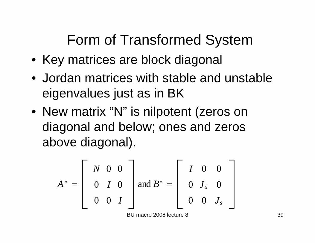
Form of Transformed Systemy• Key matrices are block diagonal

Jordan matrices ith stable and nstable• Jordan matrices with stable and unstable eigenvalues just as in BK

• New matrix “N” is nilpotent (zeros on diagonal and below; ones and zeros above diagonal).

N 0 0 I 0 0A∗

N 0 0

0 I 0

0 0 I

and B∗ I 0 0

0 Ju 0

0 0 JBU macro 2008 lecture 8 39

0 0 I 0 0 Js

An asideAn aside• Solutions to |Az-B|=0 are

called “generalizedcalled generalized eigenvalues of A,B”

• Since roots of the polynomial are not affected by

lti li ti b bit

0 0 0

0 1 0 A∗

⎡ ⎤⎢ ⎥⎢ ⎥= ⎢ ⎥multiplication by arbitrary

nonsingular matrices, these are the same as “generalized eigenvalues of A*,B*” i.e., the

t f |A* B*| 0

0 1 0

0 0 1

A = ⎢ ⎥⎢ ⎥⎢ ⎥⎢ ⎥⎣ ⎦

roots of |A*z-B*|=0.• With a little work, you can see

that there are only as many roots as n(Ju)+n(Js), since

1 0 0

0 0B∗

⎡ ⎤⎢ ⎥⎢ ⎥( ) ( ),

there are zeros on the diagonal of N. Try the case at right for intuition

0 0

0 0

u

s

B μ

μ

∗ ⎢ ⎥= ⎢ ⎥⎢ ⎥⎢ ⎥⎢ ⎥⎣ ⎦


⎢ ⎥⎣ ⎦

ImplicationsImplications

• There are transformed variables whichThere are transformed variables which evolve according to separated equation systemssystems

Yt∗

it

ut

st


Some parts are just a repeat of l f i lresults from nonsingular case

• Unstable canonical variablesUnstable canonical variables

1 0 1 1t t u t u t u t tE u J u C X C E X∗ ∗+ += + +

1 10 1 1[ ] { }h

t u t u t h u t t hu J E C X C E X∞

− + ∗ ∗+ + +⇒ = − +∑

• Stable canonical variables

0h=

Stable canonical variablesEtst1 Jsst C0s

∗ Xt C1s∗ EtXt1


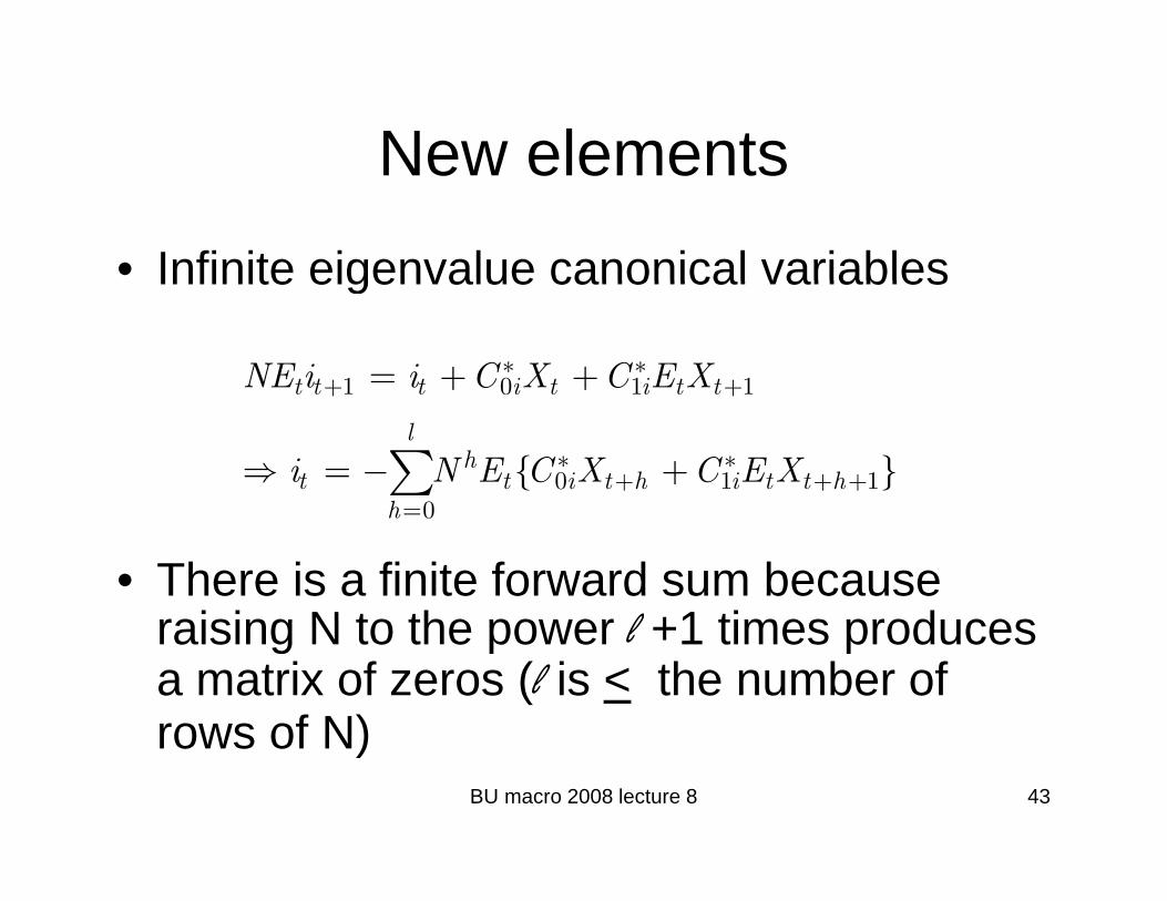
New elementsNew elements

• Infinite eigenvalue canonical variablesInfinite eigenvalue canonical variables

1 0 1 1t t t i t i t tNE i i C X C E X∗ ∗+ += + +1 0 1 1

0 1 10

{ }

t t t i t i t t

lh

t t i t h i t t hh

i N E C X C E X

+ +

∗ ∗+ + +⇒ = − +∑

• There is a finite forward sum because raising N to the power l +1 times produces

0h=

raising N to the power l +1 times produces a matrix of zeros (l is < the number of rows of N)


rows of N)

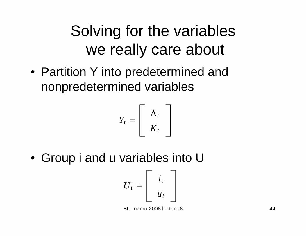
Solving for the variablesll bwe really care about

• Partition Y into predetermined andPartition Y into predetermined and nonpredetermined variables

Yt t

Kt

• Group i and u variables into Up

Ut it


ut

Partition the variable transformation i V d i i Rmatrix V and its inverse R

U

VU VUK

s

Vs VsK K

K

RU Rs

R R

U

K RKU RKs s


In a similar fashion to earlierIn a similar fashion to earlier

• We solve for nonpredetemined variablesWe solve for nonpredetemined variables given solutions for U.

1[ ]t U t UK tV U V K−ΛΛ = −

Thi i d i l

[ ]t U t UK tΛ

• This requires a square and nonsingular matrix, as in discussion of BK (same counting rule)


counting rule).

Solving for predetermined variables• Use the reverse transform, the solution for

the stable variables, and the solution for ,the U variables (unstable and infinite cvs)

Kt1 RKUEtUt1 RKsEtst1Kt1 RKUEtUt1 RKsEtst1

RKUEtUt1 RKsJsst C0s∗ Xt C1s

∗ EtXt1

RKUEtUt1 RKsJsVst VsKKtRKUEtUt1 RKsJsVst VsKKt

RKsC0s∗ Xt C1s

∗ EtXt1

RKUE U 1 RKUEtUt1

RKsJsVsVU−1 Ut − VUKKt VsKKt

R C∗ X C∗ E X


RKsC0sXt C1sEtXt1

SummarySummary

• We now have a precise solution for aWe now have a precise solution for a richer model, which incorporates prior work as special case.p

• Solvability requires |Az-B| is nonzero for some z, which is easy to check on ycomputer.

• Unique solvability requires that a certain q y qmatrix be square and invertible: counting rule is necessary condition.


Linking the two systemsLinking the two systems• KW (2003) show that any uniquely solvable ( ) y q y

model has a reduced dimension nonsingular system representation

F

F1

( )

( )

t t f t t

t t t d t t

f Kd E X

E d Wd E X+

= − − Ψ

= − Ψ

• F is lead operator (see homework)• d is a vector containing all predetermined

1 ( )t t t d t t+

• d is a vector containing all predetermined variables and some nonpredetermined variables

• There are as many “f” as “I” variablesBU macro 2008 lecture 8 49

There are as many f as I variables.

D A (Recalcitrant) ExampleD. A (Recalcitrant) Example• BK discuss an example of a model which p

their method cannot solve, which takes the form of

Eθ φ+

in the notation of this lecture. We note that this model has a natural solution unless

1t t t ty E y xθ φ−= +

this model has a natural solution, unless θ=1, which is that

φ

but that the BK approach cannot produce it.

11t t t ty E x xφ

φθ −= +

−


pp p

Casting this model in Fi O d FFirst-Order Form

• Defining wt =Et 1yt we can write this modelDefining wt =Et-1yt, we can write this model in the standard form as

1

1

0 0 1

1 1 0 0 0

t t

t tt t

y yE xw w

θ φ+

+

−⎡ ⎤ ⎡ ⎤⎡ ⎤ ⎡ ⎤ ⎡ ⎤⎢ ⎥ ⎢ ⎥⎢ ⎥ ⎢ ⎥ ⎢ ⎥= +⎢ ⎥ ⎢ ⎥⎢ ⎥− ⎢ ⎥ ⎢ ⎥⎣ ⎦ ⎣ ⎦⎢ ⎥ ⎢ ⎥ ⎢ ⎥⎣ ⎦ ⎣ ⎦ ⎣ ⎦

where the first equation is the model qabove and the second is wt+1 =Etyt+1.

• Note that |A|=0 and |B|=0BU macro 2008 lecture 8 51

Note that |A| 0 and |B| 0

The necessary conditionThe necessary condition

• Not easy to think about general meaning ofNot easy to think about general meaning of “there exists some z for which |Az-B| isn’t 0”

• But in this case it is intuitive: evaluating |Az-g |B| as we will on the next page says the condition is satisfied unless 1= θ in which case the model becomes degenerate in that it imposes restrictions on x but not on y!

E φ+1

1 1 1

t t t t

t t t t t t

y E y x

E y E y E x

φ

φ−

− − −

= +

⇒ = +


10 t tE xφ −⇒ =

Generalized eigenvaluesGeneralized eigenvalues

• Looking for finite 0 0 1| | | |A B

θ−⎡ ⎤⎡ ⎤⎢ ⎥⎢ ⎥Looking for finite

eigenvalues: z=0 is a root of |Az-B|

0 | | | |1 1 0 0

1| | (1 )

Az B z

zz z

θθ

⎢ ⎥⎢ ⎥= − = − ⎢ ⎥⎢ ⎥−⎢ ⎥ ⎢ ⎥⎣ ⎦ ⎣ ⎦−⎡ ⎤

⎢ ⎥= = − −⎢ ⎥| |

• Looking for infinite

z z⎢ ⎥−⎣ ⎦

0 01 θ−⎡ ⎤ ⎡ ⎤Looking for infinite eigenvalues: z=0 is a root of |Bz-A|

0 010 | | | |

1 10 0

| | (1 )

Bz A z

z zz

θ

θθ

⎡ ⎤ ⎡ ⎤⎢ ⎥ ⎢ ⎥= − = −⎢ ⎥ ⎢ ⎥−⎢ ⎥⎢ ⎥ ⎣ ⎦⎣ ⎦

−⎡ ⎤⎢ ⎥= = − −⎢ ⎥| | (1 )

1 1z θ= =⎢ ⎥−⎢ ⎥⎣ ⎦


General meaningGeneral meaning

• Infinite eigenvalue: there is a dynamic identityInfinite eigenvalue: there is a dynamic identity present in the model

• Zero eigenvalue: it may not be necessary to g y yhave as many state variables as predetermined variables.

• Let’s see how this can be seen in this model. We can “substitute out” the equation for y in the

i f d i i f hequation for w, producing a new version of the system which looks like that on the next page


“Reduced” System in ExampleReduced System in Example

• FeaturesFeatures– One identity

One “possibly redundant” state– One possibly redundant state• Subtlety of redundancy

1 10

t t t

t t t t

y w x

w w E x

θ φ

φ+ +

= +

= +1 101t t t tw w E x

θ+ += +−


CommentsComments

• Muth’s model 1 was easy for him but hardMuth s model 1 was easy for him, but hard from perspective of BK: it is essentially the model that we just studiedmodel that we just studied.

• Nearly every linear model that we write down is singular For example Muth’sdown is singular. For example, Muth s model 2 is singular if we do not use supply=demand to drop flow output (y) butsupply=demand to drop flow output (y), but instead want to carry it along.


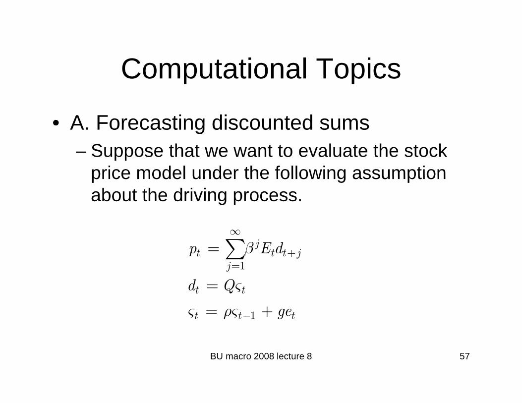
Computational TopicsComputational Topics

• A Forecasting discounted sumsA. Forecasting discounted sums– Suppose that we want to evaluate the stock

price model under the following assumptionprice model under the following assumption about the driving process.

1

jt t t j

j

p E dβ∞

+=

= ∑

1

t t

t t t

d Q

ge

ς

ς ρς −

=

= +


Working out the matrix sumWorking out the matrix sum

1 1

j jt t t j t t j

j j

p E d QEβ β ς∞ ∞

+ += =

= =∑ ∑

1 1

[ ]j j j jt t

j j

Q Qβ ρ ς β ρ ς∞ ∞

= == =∑ ∑

2

1

[ ( ) ( ) ....]

[ ( )]

j j

tQ I

Q I

βρ βρ βρ ς

βρ βρ ς−

= + + +

= [ ( )] tQ Iβρ βρ ς= −


In wordsIn words• Solution above tells how forward-looking asset price g p

depends on the state variables which govern demand.• Solution above is a very convenient formula to

implement on computer, in context of empirical work orimplement on computer, in context of empirical work or quantitative modeling

• Solution strategy generalizes naturally to evaluating forward looking components of RE models These areforward-looking components of RE models. These are, essentially, just “lots of equations with unstable eigenvalues” although frequently the sums start with 0 rather than 1 so that the details on the prior page arerather than 1, so that the details on the prior page are slightly different.


More preciselyMore precisely,• We know that solutions above include

“expected distributed leads” of xexpected distributed leads of x.• We can evaluate these given a forcing

lik th t bprocess like that above.• The result is then that the SOLUTION to

the RE model evolves as a state space system.


Additional detailAdditional detail

• Evaluating model requires we solve forEvaluating model requires we solve for 1 1

0 1 10

[ ] { }ht u t u t h u t t h t

h

u J E C X C E X ς∞

− + ∗ ∗+ + +

== − + = Φ∑

• Know all of the forecasts depend just on state so answer must have form above

0h=

state, so answer must have form above.• Algebra of working this out is similar to

stock price example above (distributedstock price example above (distributed lead starts at 0 here rather than 1, though).


though).

Full solutionFull solution• Takes the form

Yt St

S MS Ge

• With

St MSt−1 Get

K⎡ ⎤tt

t

KS ς

⎡ ⎤⎢ ⎥= ⎢ ⎥⎣ ⎦

• In words: states of solved model are predetermined variables plus the forcing (driving forecasting) variables


(driving, forecasting) variables.

Modern computational approaches make it t h dl l li RE d leasy to handle large linear RE models

• Approaches based on numerically desirableApproaches based on numerically desirable versions (called QZ) of the TV transformations described above– Klein (JEDC)– Sims (Computational Economics, 2003)

• Approaches based on finding a subsytem or otherwise reducing the dimension of problem

AIM (A d d M FRBG)– AIM (Anderson and Moore at FRBG)– King/Watson (Computational Economics, 2003)

Sargent and coauthorsBU macro 2008 lecture 8 63

– Sargent and coauthors

Summary• A. Core Ideas

– Recursive forward solution for nonpredetermined variables– Recursive forward solution for predetermined variablesecu s e o a d so ut o o p edete ed a ab es– Unwinding unstable roots forward

• B. Nonsingular Systems Theory– Unique stable solution requires: number of predetermined = q q p

number of unstable• C. Singular Systems Theory

– Solvability: |Az-B| nonzero plus counting rule• D. A Singular Systems Example

– Solvability condition interpreted• E. Computationp

– With state space driving process, solution to model occurs in state space form

– States are predetermined variables (the past) and driving variables (the present and future x’s)


variables (the present and future x s)

lecture 8: solving linear rationallinear rational

Documents