Solving Linear Rational Expectation Models

Dr. Tai-kuang Ho�

�Associate Professor. Department of Quantitative Finance, National Tsing Hua University, No.101, Section 2, Kuang-Fu Road, Hsinchu, Taiwan 30013, Tel: +886-3-571-5131, ext. 62136, Fax:+886-3-562-1823, E-mail: tkho@mx.nthu.edu.tw. This lecture note is based on Klein�s paper and

1 The problem

� Approaches to solve linear rational expectation models include Sims (2002), An-derson and Moore (1985), Binder and Pesaran (1994), King and Watson (1998),Klein (2000), and Uhlig (1999).

� A recent view is Anderson (2008), who compares the accuracy and computationalspeed of alternative approaches to solving linear rational expectations models.

� Martin Uribe�s Lectures in Open Economy Macroeconomics, Appendix of Chapter4, provides a very clear explanation of the linear solution method to dynamicgeneral equilibrium models.

Fabrice Collard�s lecture note. The latter contains many typos and I have tried my best to make theyright in this document.

� Martin Uribe�s Lectures are available from his website.

� McCandless, George (2008), The ABCs of RBCs: An Introduction to DynamicMacroeconomic Models, Harvard University Press.

� This book provides an detailing introduction to solving dynamic stochastic gen-eral equilibrium model.

� It is very practical for beginners as the author explains the deduction step bystep, and the book includes many examples and solutions that facilitate learning.

� The author uses �rst-order approximation to the model, and adopts Uhlig�s toolk-its and related computer programs to solve the log-linearized model.

� Klein (2000) uses a complex generalized Schur decomposition to solve linearrational expectation models.

� Why generalized Schur decomposition?

� First, it treats in�nite and �nite unstable eigenvalues in a uni�ed way.

� Second, Schur decomposition is computationally more preferable.

� Setting the stage

� Measurement equation, which describe variables of interest, such as output orgross interest rate.

NyYt = NxXt +NzZt (1)

� Endogenous variables

Mx0EtXt+1 +My0EtYt+1 +Mz0EtZt+1 =Mx1Xt +My1Yt +Mz1Zt (2)

� Exogenous shocks (forcing variables)

Zt = �Zt�1 +�t (3)

� Dimension of variables

Yt : ny � 1Xt : nx � 1Zt : nz � 1

� Predetermined variables Xbt : nb

� Jump (control) variables Xft : nf

� nx = nb + nf

Xt =�XbtXft

�

� Dimension of matrices

Ny(ny � ny)

Nx(ny � nx)

Nz(ny � nz)

Mx0(nx � nx)

My0(nx � ny)

Mz0(nx � nz)

Mx1(nx � nx)

My1(nx � ny)

Mz1(nx � nz)

�(nz � nz)

(nz � ne)

� Ny is invertible, which means that the variable of interest is uniquely de�ned.

� All eigenvalues of � lies within the unit circle

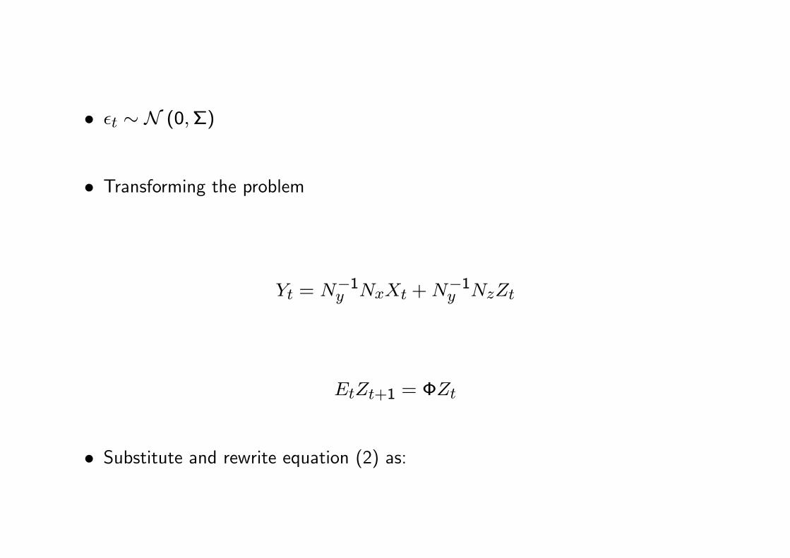
� �t � N (0;�)

� Transforming the problem

Yt = N�1y NxXt +N

�1y NzZt

EtZt+1 = �Zt

� Substitute and rewrite equation (2) as:

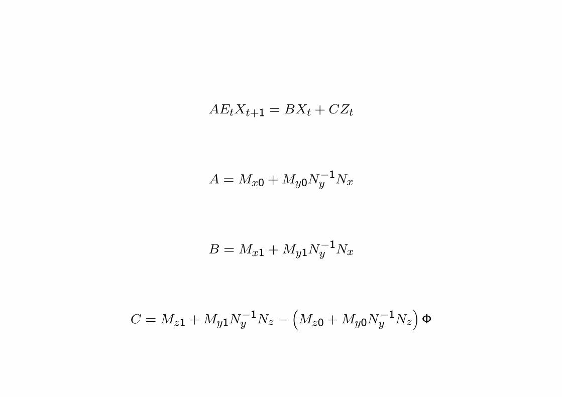
AEtXt+1 = BXt + CZt

A =Mx0 +My0N�1y Nx

B =Mx1 +My1N�1y Nx

C =Mz1 +My1N�1y Nz �

�Mz0 +My0N

�1y Nz

��

� This system comes from the linearization of the individual optimization conditionsand market clearing conditions in a dynamic equilibrium model.

� The matrix A is allowed to be singular.

� A singular matrix A implies that static (intra-temporal) equilibrium conditionsare included among the dynamic relationships.

2 Generalized Schur decomposition

� The idea of Klein�s approach is to use complex generalized Schur decompositionto reduce the system into an unstable and a stable block of equations.

� The stable solution is found by solving the unstable block forward and the stableblock backward.

De�nition of predetermined or backward-looking variables: a process k is calledbackward-looking if the prediction error �t+1 � kt+1�Etkt+1 is an exogenousmartingale di¤erence process (Et�t+1 = 0) and k0 is exogenous given.

� The dynamic equation

AEtXt+1 = BXt + CZt

� Generalized Schur decomposition of the pencil (A;B)

S = QAZ

T = QBZ

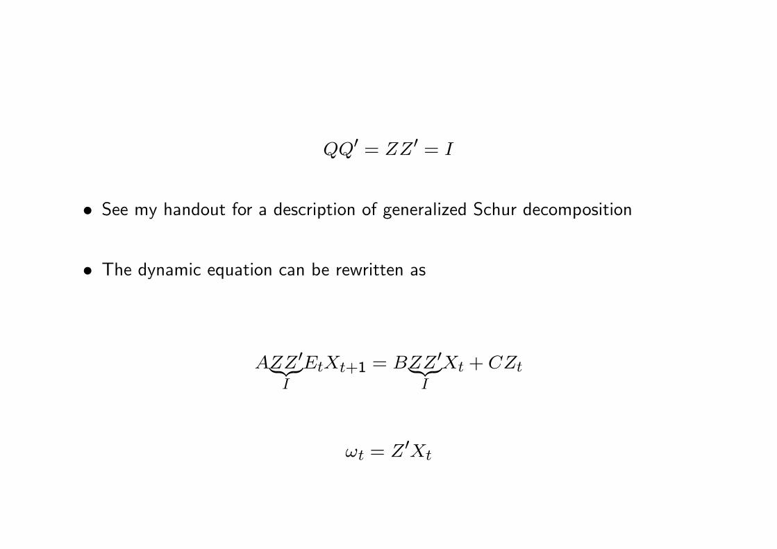
QQ0 = ZZ0 = I

� See my handout for a description of generalized Schur decomposition

� The dynamic equation can be rewritten as

AZZ0| {z }I

EtXt+1 = BZZ0| {z }

I

Xt + CZt

!t = Z0Xt

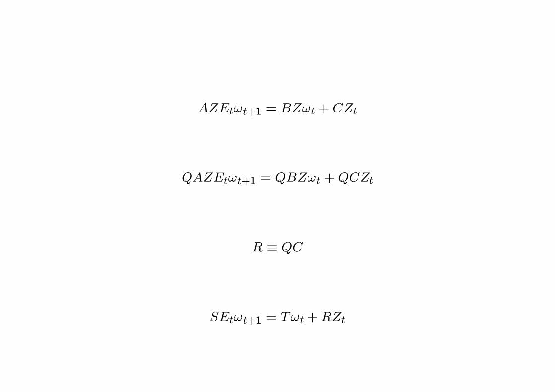
AZEt!t+1 = BZ!t + CZt

QAZEt!t+1 = QBZ!t +QCZt

R � QC

SEt!t+1 = T!t +RZt

� Don�t confuse Z with Zt.

� Remark

Z =

Z11 Z12Z21 Z22

!

!t = Z0Xt =

"Z011 Z021Z012 Z022

# "XbtXft

#=

24Z011Xbt + Z021XftZ012X

bt + Z

022X

ft

35 � "!bt!ft

#

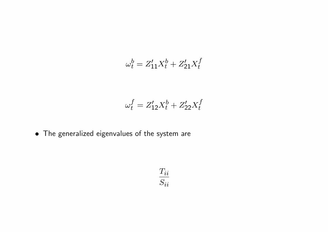
!bt = Z011X

bt + Z

021X

ft

!ft = Z

012X

bt + Z

022X

ft

� The generalized eigenvalues of the system are

TiiSii

� We sort the generalized eigenvalues in ascending order.

� ns stable eigenvalues

� nu unstable eigenvalues

Blanchard and Kahn condition: if nb = ns (and nf = nu) then the system admitsa unique saddle path.

� There are as many predetermined variables as there are stable eigenvalues.

� How likely is that nb = ns?

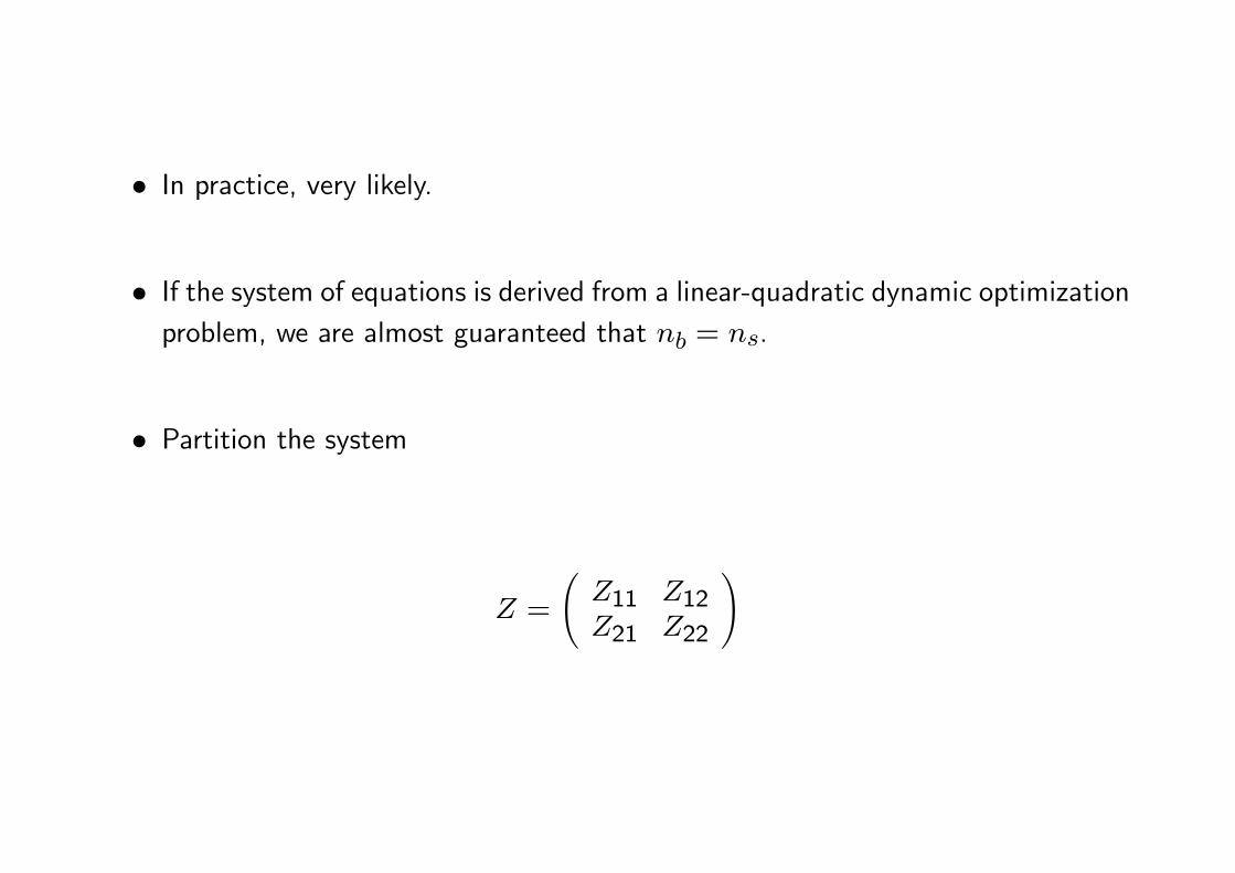
� In practice, very likely.

� If the system of equations is derived from a linear-quadratic dynamic optimizationproblem, we are almost guaranteed that nb = ns.

� Partition the system

Z =

Z11 Z12Z21 Z22

!

S =

S11 S120 S22

!

T =

T11 T120 T22

!

Z11 : ns � nsZ12 : ns � nfZ21 : nf � nsZ22 : nf � nf

� Rewrite the system as

S11 S120 S22

!0@ Et!bt+1

Et!ft+1

1A = T11 T120 T22

! !bt!ft

!+

R1R2

!Zt

� S11 and T22 are invertible by construction.

3 The forward part of the solution

� Look at the unstable part of the system

S22Et!ft+1 = T22!

ft +R2Zt

!ft = T

�122 S22Et!

ft+1 � T

�122 R2Zt

!ft = lim

k!1

�T�122 S22

�kEt!

ft+k �

1Xk=0

�T�122 S22

�kT�122 R2�

kZt

Et!ft+k <1

limk!1

�T�122 S22

�kEt!

ft+k = 0

!ft = �

1Xk=0

�T�122 S22

�kT�122 R2�

kZt = �Zt

� � �1Xk=0

�T�122 S22

�kT�122 R2�

k

� Some matrix algebraic

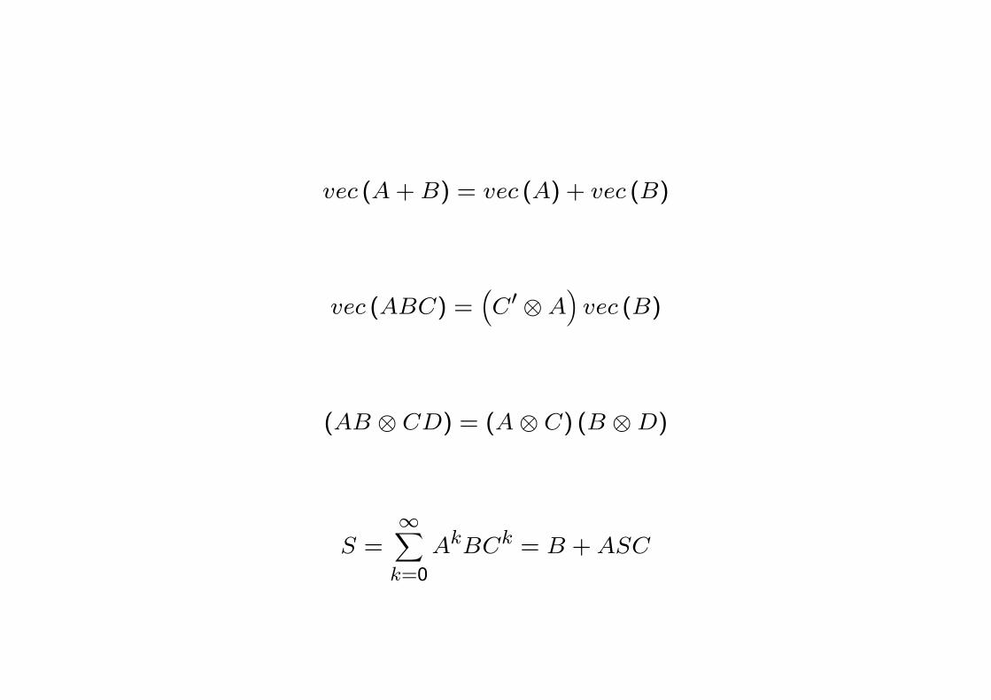
vec (A+B) = vec (A) + vec (B)

vec (ABC) =�C0 A

�vec (B)

(AB CD) = (A C) (B D)

S =1Xk=0

AkBCk = B +ASC

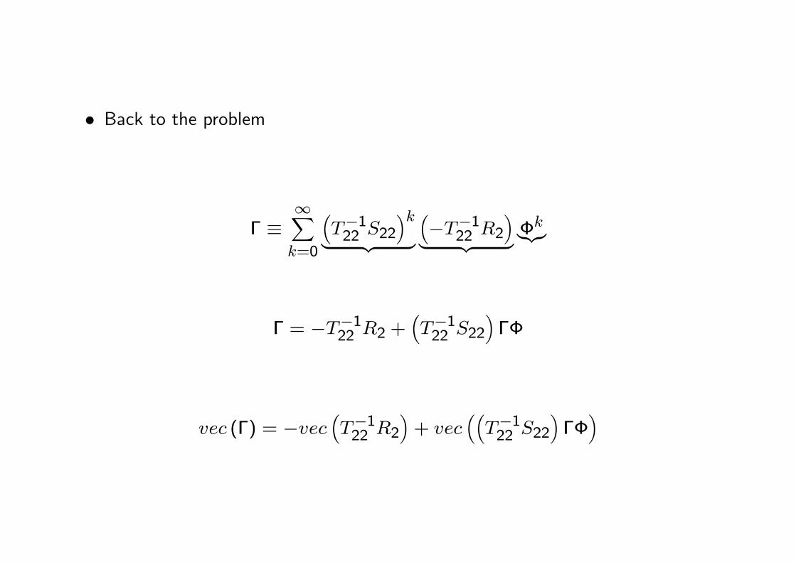
� Back to the problem

� �1Xk=0

�T�122 S22

�k| {z }��T�122 R2

�| {z } �k|{z}

� = �T�122 R2 +�T�122 S22

���

vec (�) = �vec�T�122 R2

�+ vec

��T�122 S22

����

vec (�) = ��I T�122

�vec (R2) +

��0

�T�122 S22

��vec (�)

vec (�) = ��I T�122

�vec (R2) +

��0 T�122

�(I (S22)) vec (�)

(I T22) vec (�) = �vec (R2) +��0 S22

�vec (�)

vec (�) =��0 S22 � I T22

��1vec (R2)

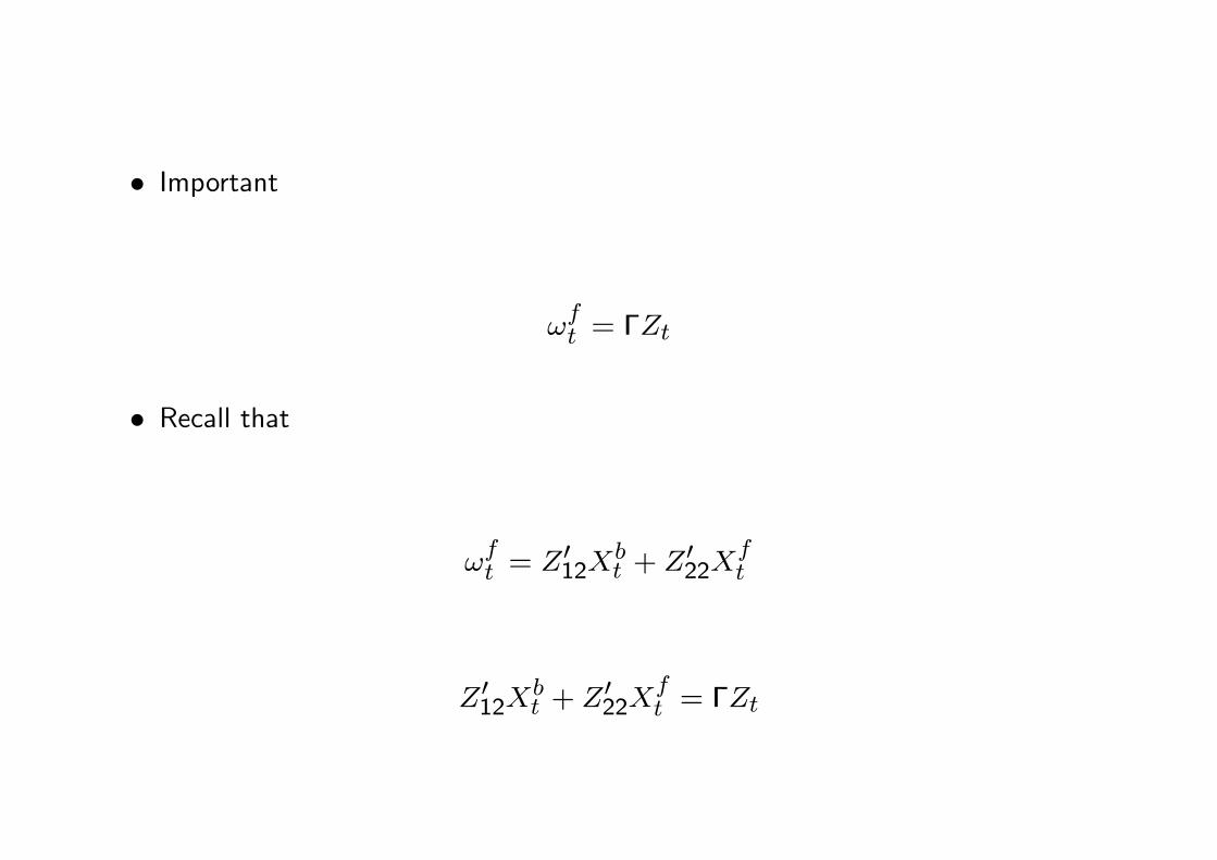
� Important

!ft = �Zt

� Recall that

!ft = Z

012X

bt + Z

022X

ft

Z012Xbt + Z

022X

ft = �Zt

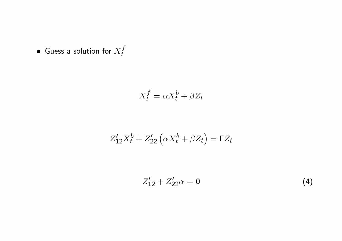
� Guess a solution for Xft

Xft = �X

bt + �Zt

Z012Xbt + Z

022

��Xbt + �Zt

�= �Zt

Z012 + Z022� = 0 (4)

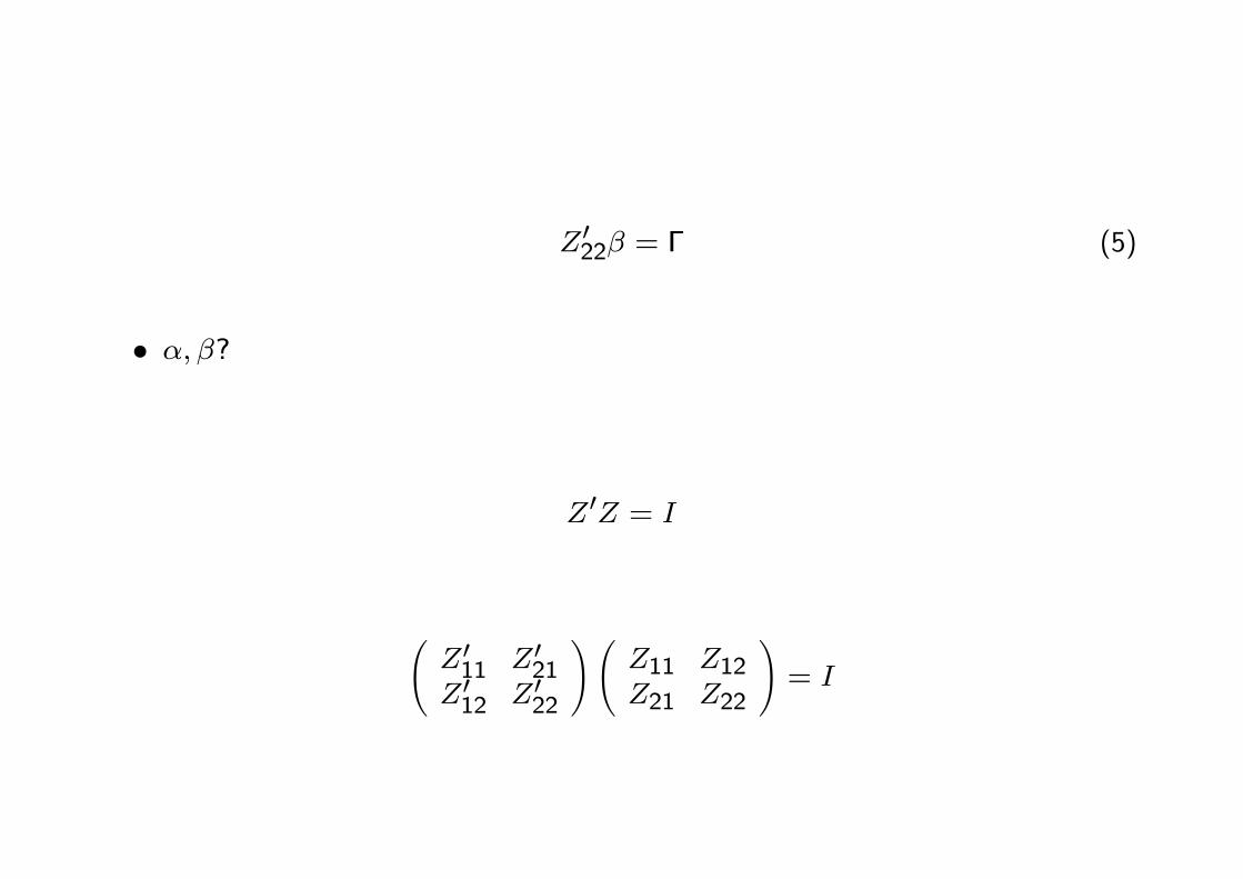
Z022� = � (5)

� �; �?

Z0Z = I

Z011 Z021Z012 Z022

! Z11 Z12Z21 Z22

!= I

"Z011Z11 + Z

021Z21 Z011Z12 + Z

021Z22

Z012Z11 + Z022Z21 Z012Z12 + Z

022Z22

#=

"I 00 I

#

Z012Z11 + Z022Z21 = 0

Z012 + Z022Z21Z

�111 = 0

� Recall equation (4)

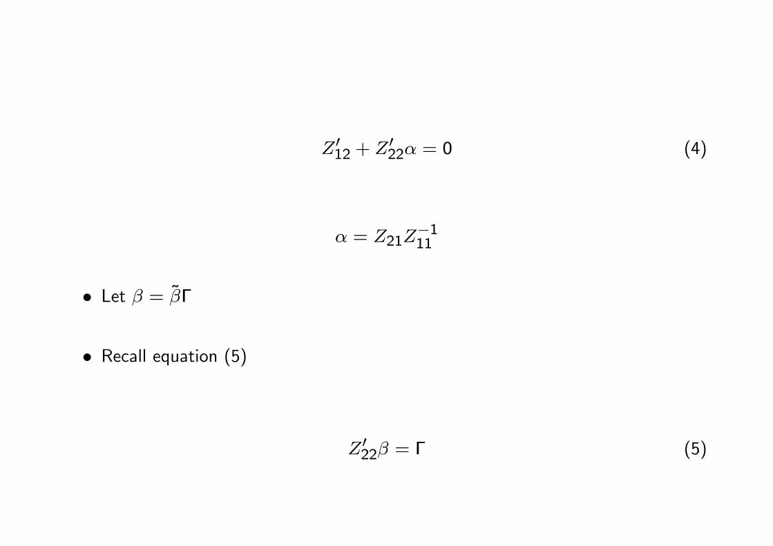
Z012 + Z022� = 0 (4)

� = Z21Z�111

� Let � = ~��

� Recall equation (5)

Z022� = � (5)

Z022� = �

Z022~�� = �

Z012Z11 + Z022Z21 = 0

Z012 = �Z022Z21Z�111

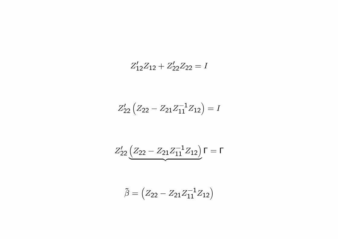
Z012Z12 + Z022Z22 = I

Z022�Z22 � Z21Z�111 Z12

�= I

Z022�Z22 � Z21Z�111 Z12

�| {z } � = �

~� =�Z22 � Z21Z�111 Z12

�

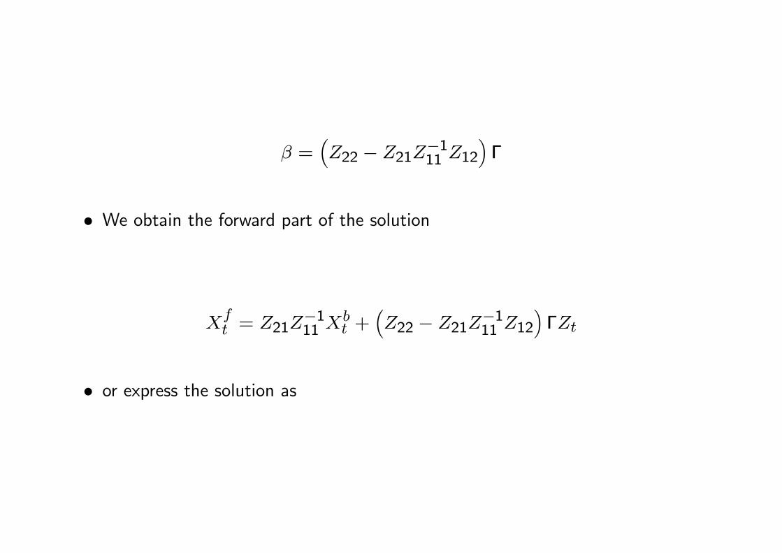
� =�Z22 � Z21Z�111 Z12

��

� We obtain the forward part of the solution

Xft = Z21Z

�111 X

bt +

�Z22 � Z21Z�111 Z12

��Zt

� or express the solution as

Xft = FxX

bt + FzZt

Fx � Z21Z�111

Fz ��Z22 � Z21Z�111 Z12

��

vec (�) =��0 S22 � I T22

��1vec (R2)

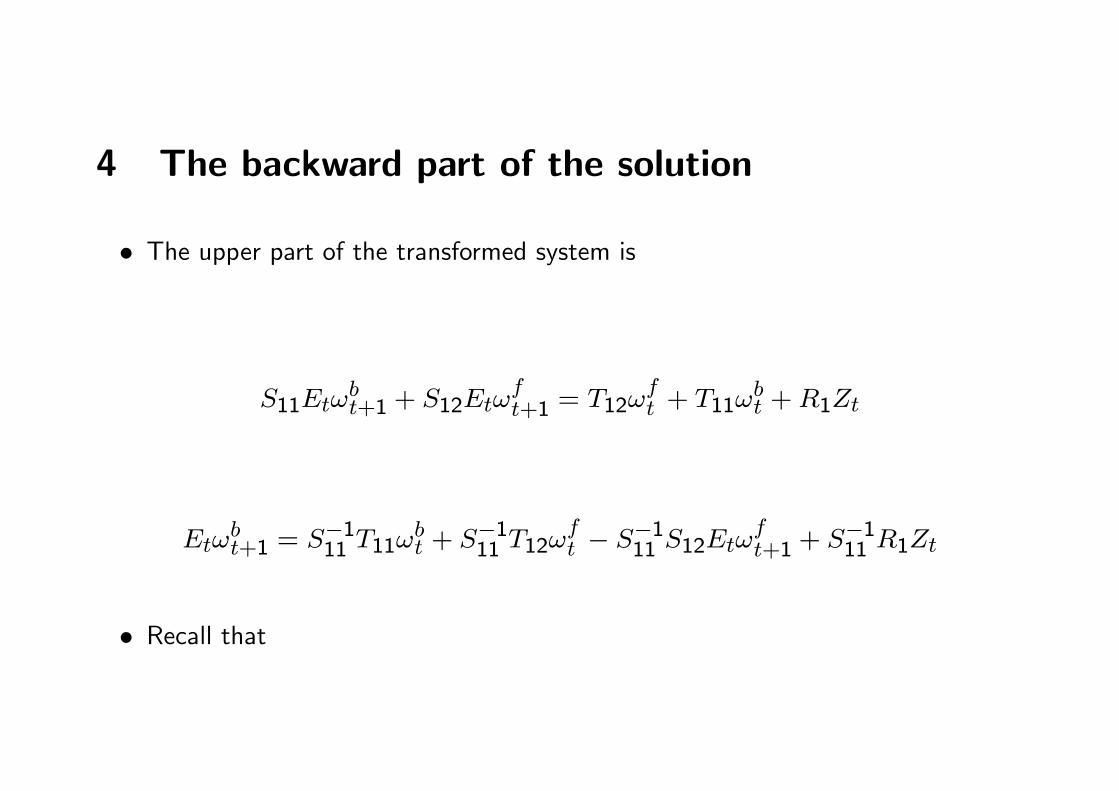
4 The backward part of the solution

� The upper part of the transformed system is

S11Et!bt+1 + S12Et!

ft+1 = T12!

ft + T11!

bt +R1Zt

Et!bt+1 = S

�111 T11!

bt + S

�111 T12!

ft � S

�111 S12Et!

ft+1 + S

�111 R1Zt

� Recall that

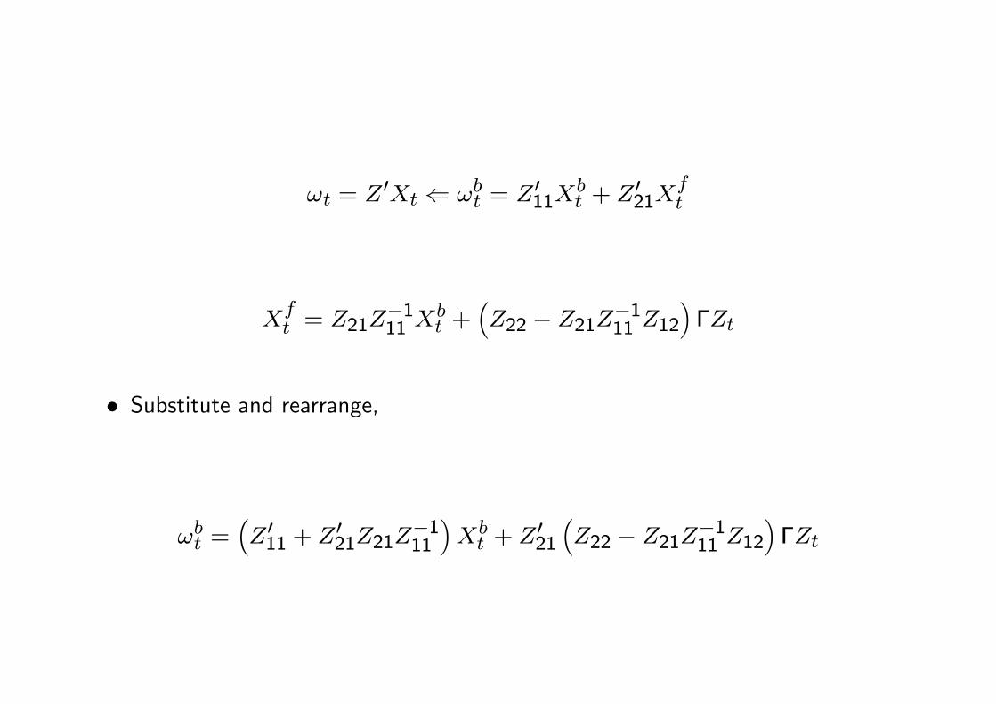
!t = Z0Xt ( !bt = Z

011X

bt + Z

021X

ft

Xft = Z21Z

�111 X

bt +

�Z22 � Z21Z�111 Z12

��Zt

� Substitute and rearrange,

!bt =�Z011 + Z

021Z21Z

�111

�Xbt + Z

021

�Z22 � Z21Z�111 Z12

��Zt

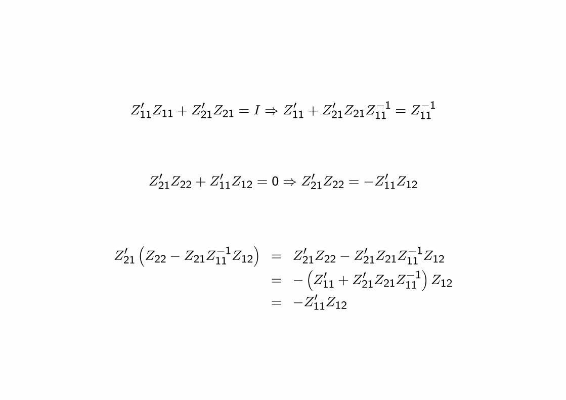
Z011Z11 + Z021Z21 = I ) Z011 + Z

021Z21Z

�111 = Z

�111

Z021Z22 + Z011Z12 = 0) Z021Z22 = �Z011Z12

Z021�Z22 � Z21Z�111 Z12

�= Z021Z22 � Z021Z21Z�111 Z12= �

�Z011 + Z

021Z21Z

�111

�Z12

= �Z011Z12

!bt = Z�111 X

bt � Z�111 Z12�Zt

Z�111 Xbt = !

bt + Z

�111 Z12�Zt

Xbt = Z11!bt + Z11Z

�111 Z12�Zt = Z11!

bt + Z12 �Ztz }| {

= !ft

= Z11!bt + Z12!

ft

� Xbt are predetermined variables

Xbt+1 � EtXbt+1 = 0

� Klein (2000) assumes Xbt+1 � EtXbt+1 = �t+1

Xbt = Z11!bt + Z12!

ft

Xbt+1 � EtXbt+1 = 0

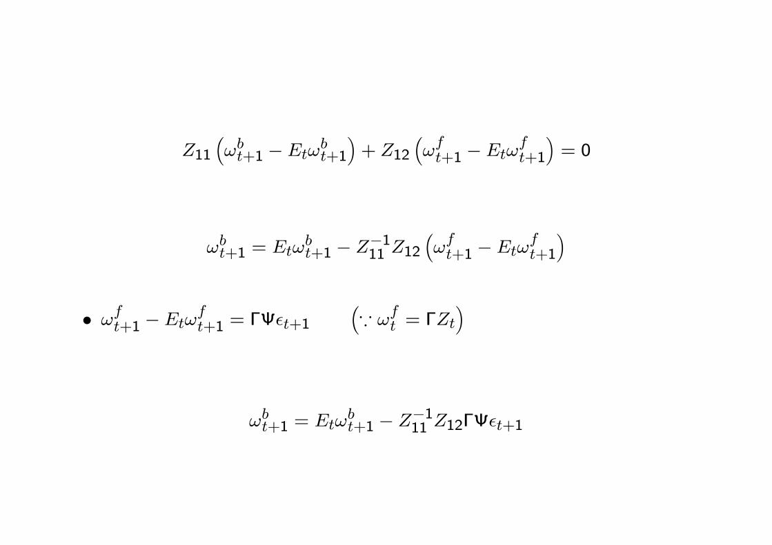
Z11�!bt+1 � Et!bt+1

�+ Z12

�!ft+1 � Et!

ft+1

�= 0

!bt+1 = Et!bt+1 � Z�111 Z12

�!ft+1 � Et!

ft+1

�

� !ft+1 � Et!ft+1 = ��t+1

�* !ft = �Zt

�

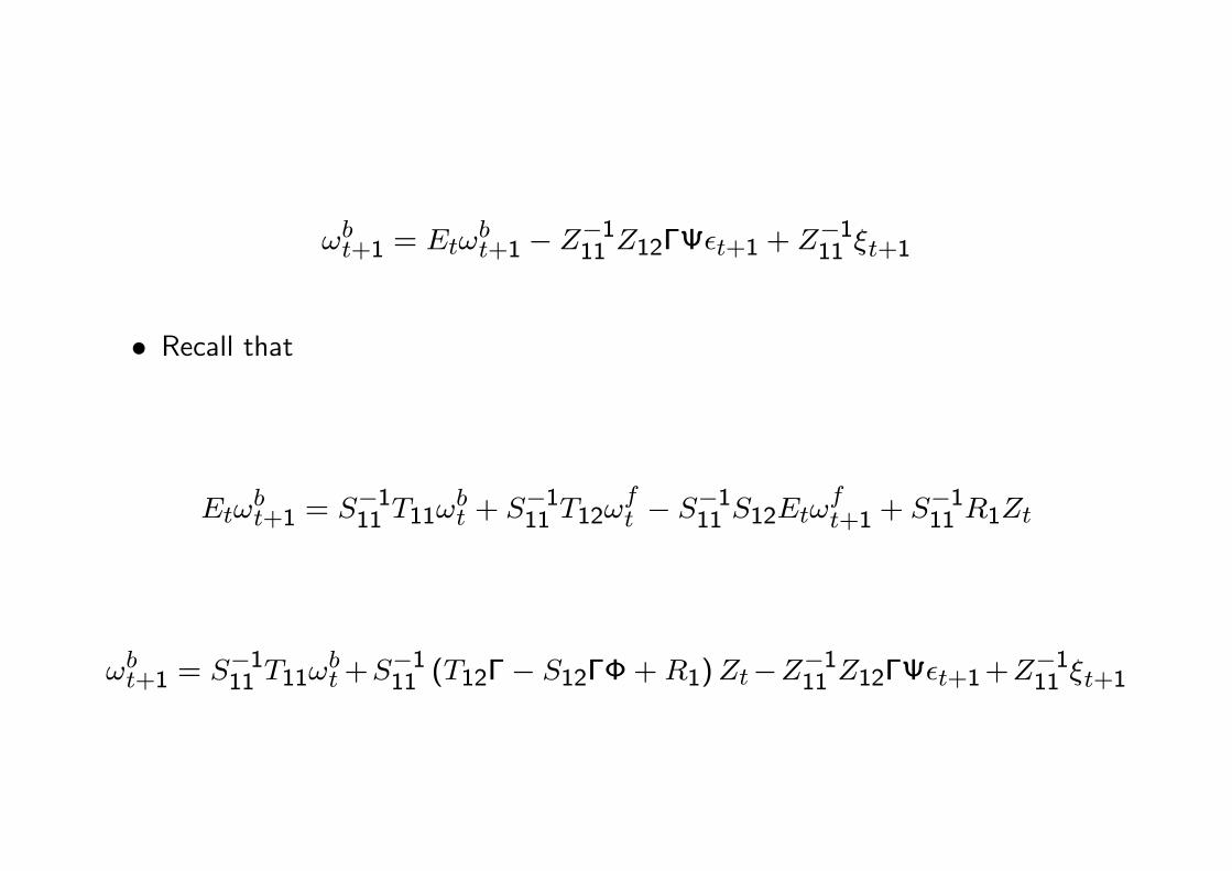
!bt+1 = Et!bt+1 � Z�111 Z12��t+1

� Recall that

Et!bt+1 = S

�111 T11!

bt + S

�111 T12!

ft � S

�111 S12Et!

ft+1 + S

�111 R1Zt

!bt+1 = S�111 T11!

bt + S

�111 (T12�� S12�� +R1)Zt � Z

�111 Z12��t+1

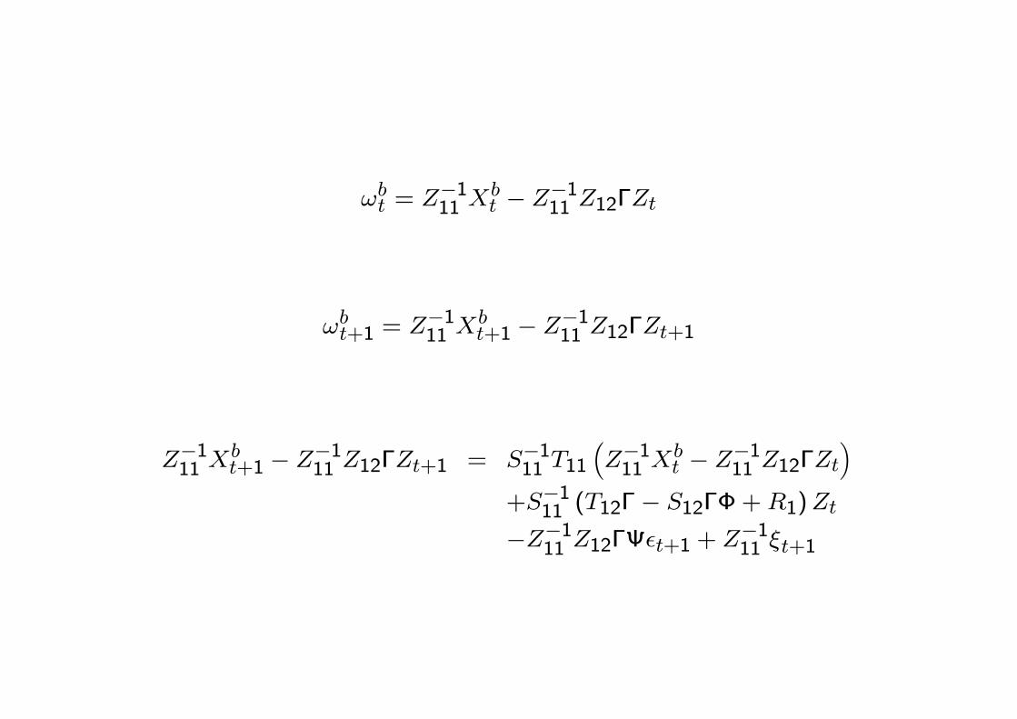
!bt = Z�111 X

bt � Z�111 Z12�Zt

!bt+1 = Z�111 X

bt+1 � Z�111 Z12�Zt+1

Z�111 Xbt+1 � Z�111 Z12�Zt+1 = S�111 T11

�Z�111 X

bt � Z�111 Z12�Zt

�+S�111 (T12�� S12�� +R1)Zt � Z

�111 Z12��t+1

Xbt+1 � Z12�Zt+1 = Z11S�111 T11

�Z�111 X

bt � Z�111 Z12�Zt

�+Z11S

�111 (T12�� S12�� +R1)Zt � Z12��t+1

Zt+1 = �Zt +�t+1

Xbt+1 = Z11S�111 T11Z

�111 X

bt

+hZ11S

�111

�T12�� S12��� T11Z�111 Z12� +R1

�+ Z12��

iZt

� The dynamics of the predetermined variables is

Xbt+1 =MxXbt +MzZt

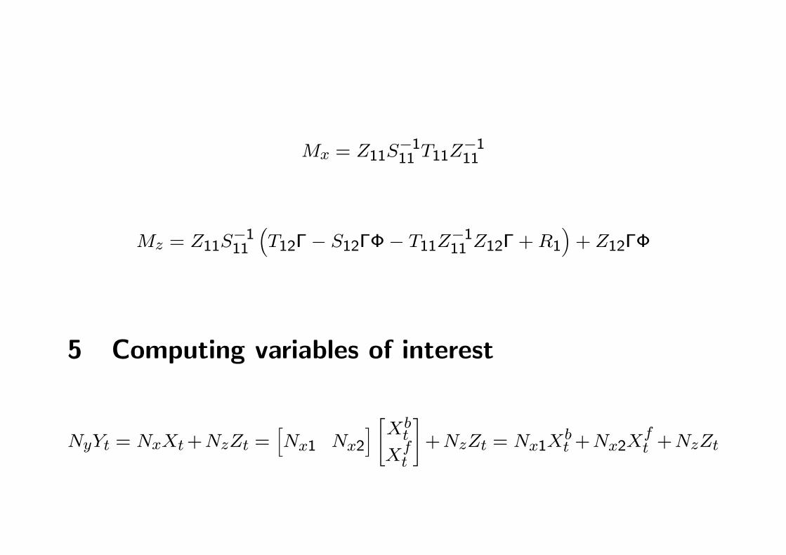
Mx = Z11S�111 T11Z

�111

Mz = Z11S�111

�T12�� S12��� T11Z�111 Z12� +R1

�+ Z12��

5 Computing variables of interest

NyYt = NxXt+NzZt =hNx1 Nx2

i "XbtXft

#+NzZt = Nx1X

bt +Nx2X

ft +NzZt

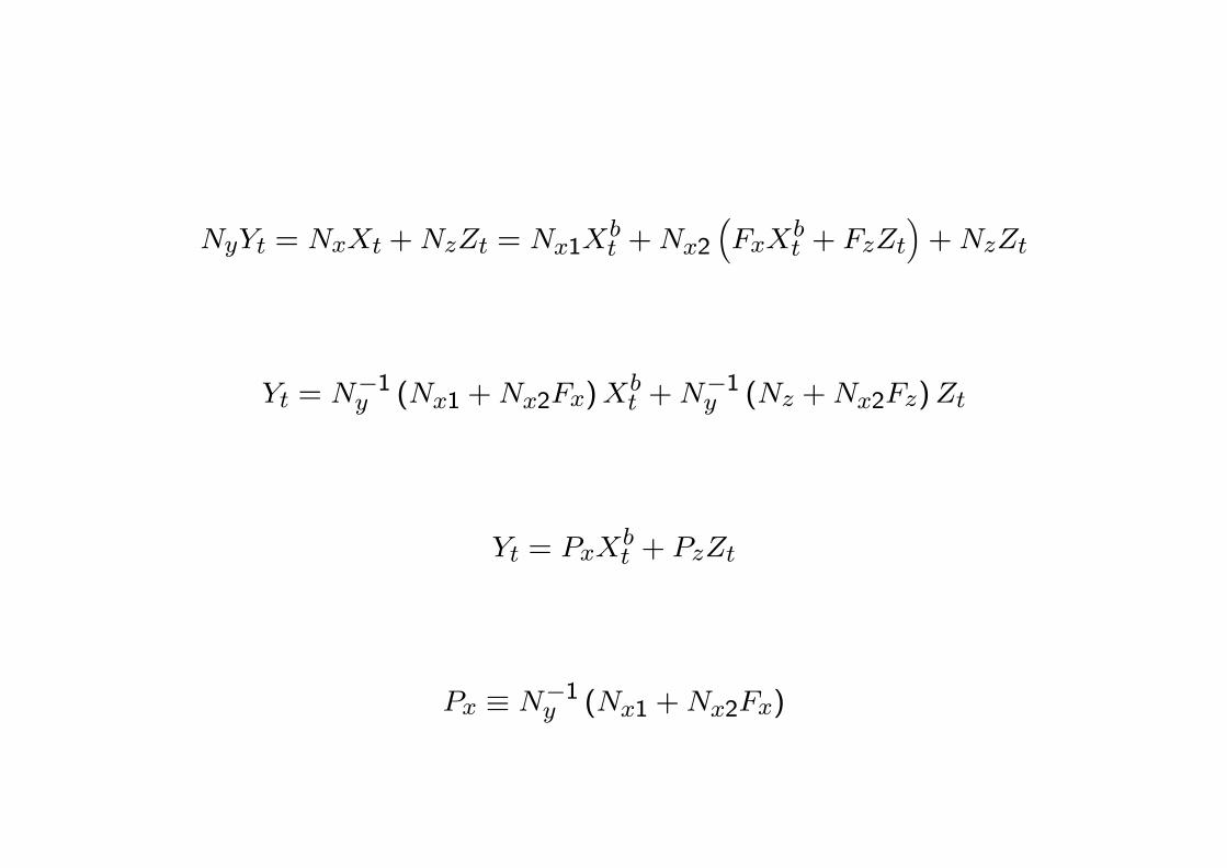
NyYt = NxXt +NzZt = Nx1Xbt +Nx2

�FxX

bt + FzZt

�+NzZt

Yt = N�1y (Nx1 +Nx2Fx)X

bt +N

�1y (Nz +Nx2Fz)Zt

Yt = PxXbt + PzZt

Px � N�1y (Nx1 +Nx2Fx)

Pz � N�1y (Nz +Nx2Fz)

� Express the solution of the whole system is state-space form

Xbt+1 =MxXbt +MzZt

Zt+1 = �Zt +�t+1

Xft = FxX

bt + FzZt

Yt = PxXbt + PzZt

6 When Xbt+1 � EtXbt+1 = �t+1

� Klein (2000) assumes Xbt+1 � EtXbt+1 = �t+1

Xbt = Z11!bt + Z12!

ft

Xbt+1 � EtXbt+1 = �t+1

Z11�!bt+1 � Et!bt+1

�+ Z12

�!ft+1 � Et!

ft+1

�= �t+1

!bt+1 = Et!bt+1 � Z�111 Z12

�!ft+1 � Et!

ft+1

�+ Z�111 �t+1

!bt+1 = Et!bt+1 � Z�111 Z12��t+1 + Z

�111 �t+1

� Recall that

Et!bt+1 = S

�111 T11!

bt + S

�111 T12!

ft � S

�111 S12Et!

ft+1 + S

�111 R1Zt

!bt+1 = S�111 T11!

bt+S

�111 (T12�� S12�� +R1)Zt�Z

�111 Z12��t+1+Z

�111 �t+1

!bt = Z�111 X

bt � Z�111 Z12�Zt

!bt+1 = Z�111 X

bt+1 � Z�111 Z12�Zt+1

Z�111 Xbt+1 � Z�111 Z12�Zt+1 = S�111 T11

�Z�111 X

bt � Z�111 Z12�Zt

�+S�111 (T12�� S12�� +R1)Zt�Z�111 Z12��t+1 + Z

�111 �t+1

Xbt+1 � Z12�Zt+1 = Z11S�111 T11

�Z�111 X

bt � Z�111 Z12�Zt

�+Z11S

�111 (T12�� S12�� +R1)Zt � Z12��t+1 + �t+1

Zt+1 = �Zt +�t+1

Xbt+1 = Z11S�111 T11Z

�111 X

bt

+hZ11S

�111

�T12�� S12��� T11Z�111 Z12� +R1

�+ Z12��

iZt + �t+1

� The dynamics of the predetermined variables is

Xbt+1 =MxXbt +MzZt + �t+1

Mx = Z11S�111 T11Z

�111

Mz = Z11S�111

�T12�� S12��� T11Z�111 Z12� +R1

�+ Z12��

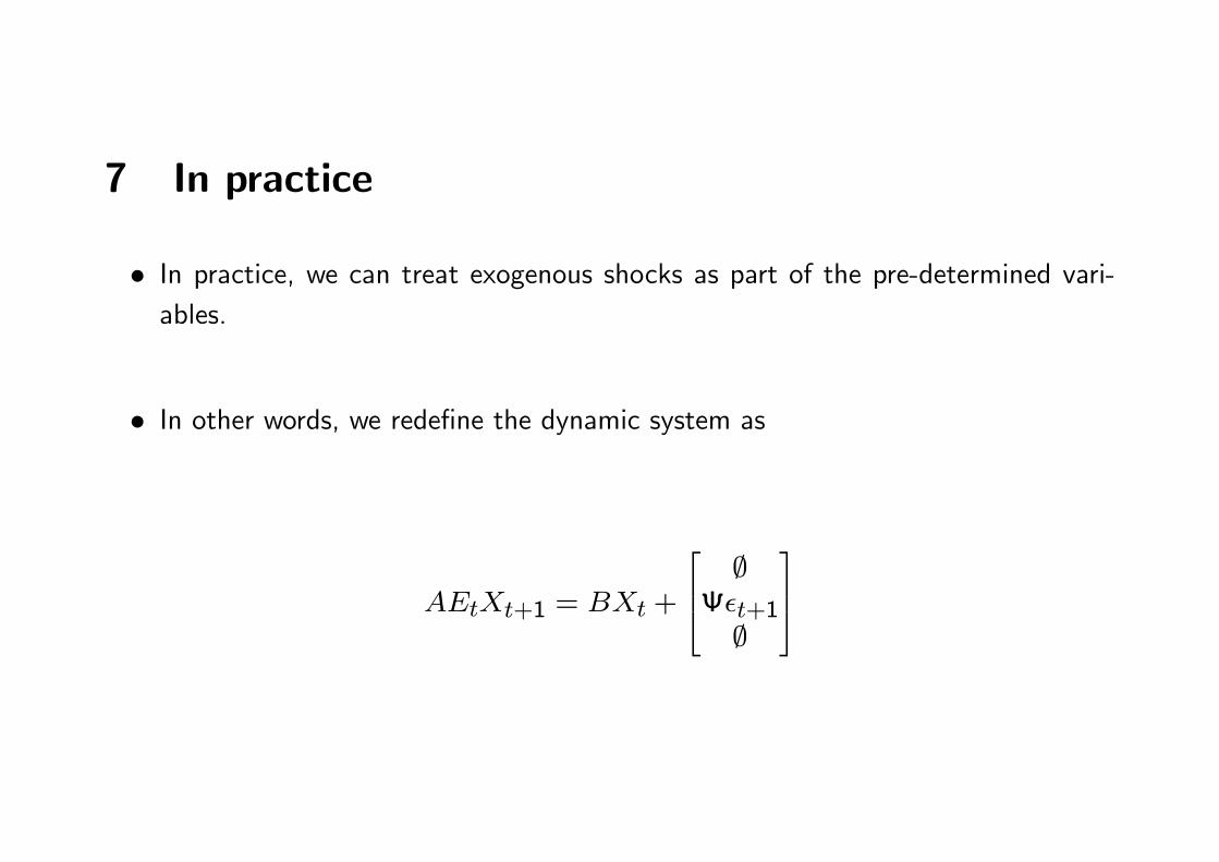
7 In practice

� In practice, we can treat exogenous shocks as part of the pre-determined vari-ables.

� In other words, we rede�ne the dynamic system as

AEtXt+1 = BXt +

264 ;�t+1;

375

Xt =

2664XbtZt

Xft

3775 �"X btXft

#

X bt �"XbtZt

#

� The solution to the system becomes

X bt+1 =MxX bt + �t+1 (6)

Mx = Z11S�111 T11Z

�111

�t+1 =

";

�t+1

#

Xft = FxX

bt (7)

Fx = Z21Z�111

� This is the solution form employed in Klein�s MATLAB code.

� To implement Paul Klein�s method, you need 3 MATLAB m �les: solab.m;qzswitch.m; and qzdiv.m.

� These MATLAB m �les are available from Paul Klein�s website.

� The 2 MATLAB m �les, qzswitch.m and qzdiv.m, are originally written by C.Sims.

References

[1] Anderson, Gary S. (2008), "Solving Linear Rational Expectations Models: A HorseRace," Computational Economics, 31, pp. 95-113.

[2] Klein, Paul (2000), "Using the generalized Schur form to solve a multivariatelinear rational expectations model," Journal of Economic Dynamics and Control,24, pp. 1405-1423.