NBER WORKING PAPER SERIES

LOCAL FISCAL MULTIPLIERS AND FISCAL SPILLOVERS IN THE UNITEDSTATES

Alan J. AuerbachYuriy Gorodnichenko

Daniel Murphy

Working Paper 25457http://www.nber.org/papers/w25457

NATIONAL BUREAU OF ECONOMIC RESEARCH1050 Massachusetts Avenue

Cambridge, MA 02138January 2019

This paper was presented at the 19th IMF Jacques Polak Annual Research Conference, November 1-2, 2018 and the American Economic Association Annual Meeting, January 4-6, 2019. We are grateful to our discussants, Christopher Erceg and Christoph Boehm, for comments on earlier drafts, and Peter McCrory, Hanna Charankevich, Jianlin Wang, and Chaoran Yu as well as Carlos Paramo, Preethan Gujjula, Naman Priyadarshi, Jeffrey Landes, Lingyun Xiao, and Mihir Gokhale for excellent research assistance. The views expressed herein are those of the authors and do not necessarily reflect the views of the National Bureau of Economic Research.

NBER working papers are circulated for discussion and comment purposes. They have not been peer-reviewed or been subject to the review by the NBER Board of Directors that accompanies official NBER publications.

© 2019 by Alan J. Auerbach, Yuriy Gorodnichenko, and Daniel Murphy. All rights reserved. Short sections of text, not to exceed two paragraphs, may be quoted without explicit permission provided that full credit, including © notice, is given to the source.

Local Fiscal Multipliers and Fiscal Spillovers in the United StatesAlan J. Auerbach, Yuriy Gorodnichenko, and Daniel MurphyNBER Working Paper No. 25457January 2019JEL No. E62,H5

ABSTRACT

We estimate local fiscal multipliers and spillovers for the United States using a rich dataset based on U.S. Department of Defense contracts and a variety of outcome variables relating to income and employment. We find strong positive spillovers across locations and industries. Both backward linkages and general equilibrium effects (e.g., income multipliers) contribute to the positive spillovers. Geographical spillovers appear to dissipate fairly quickly with distance. Our evidence points to the relevance of Keynesian-type models that feature excess capacity.

Alan J. AuerbachDepartment of Economics530 Evans Hall, #3880University of California, BerkeleyBerkeley, CA 94720-3880and NBERauerbach@econ.berkeley.edu

Yuriy GorodnichenkoDepartment of Economics530 Evans Hall #3880University of California, BerkeleyBerkeley, CA 94720-3880and IZAand also NBERygorodni@econ.berkeley.edu

Daniel MurphyDarden School of BusinessUniversity of VirginiaCharlottesville, VA 22906murphyd@darden.virginia.edu

1. Introduction

The strength of fiscal multipliers and spillovers have been the subject of intense debate and

considerable empirical research in recent years. An important part of this literature has provided

estimates of “local” fiscal multipliers, based on the effects of differential fiscal shocks at lower

levels of aggregation within larger entities, e.g., states within the United States or countries within

the European Union or the OECD. But the translation of local multipliers into national ones is not

straightforward, in part because of the potential for large fiscal spillovers, especially among entities

that are strongly integrated economically. In this paper, we contribute to the literature on local

fiscal multipliers while also providing estimates of the strength of fiscal spillovers, both geographic

and across industries, taking advantage of unique, detailed microdata on local defense spending.

Local multipliers inform estimates of national multiplier and are of independent interest to

localities that experience fiscal shocks and to neighbors of those localities. Defense spending in a

locality could crowd out private-sector output in that locality (e.g., through increased demand and

prices for local inputs, notably labor) or increase private-sector output through income multiplier

effects and upstream input-output linkages. Likewise, neighboring localities could experience an

increase in their employment/output through positive multiplier effects or they could decline as

labor inputs flow to the neighbor to accommodate the increase in demand there. An important

empirical question, which we address in this paper, is how an autonomous increase in demand in

a location/industry (a) affects employment in other industries in that location; and (b) affects

employment in nearby locations.

Understanding these spillover effects from government spending on private activity is a

fundamental and largely unresolved task in macroeconomics. While many would agree that there

are potential direct benefits from productive government spending, such as infrastructure, there is

little consensus on whether defense spending, which generally does not deliver direct local

productivity benefits, has any indirect local benefit. The lack of consensus is due in part to a dearth

of evidence. It is simply very difficult to identify and isolate exogenous changes in local

government spending. Even when such exogenous variation exists, researchers typically cannot

reject the null hypothesis that government spending crowds out the private sector (as would be

implied by aggregate closed-economy multipliers less than 1).

2

A recent influential paper by Cohen, Coval, and Malloy (2011) finds that an influx of federal

funds into a congressional district, attributable to likely exogenous political shifts, causes a reduction

in private-sector investment in that location. They propose a mechanism whereby the local spending

reduces labor available to the private sector, which drives down investment. It remains to be

determined whether an influx of federal funds (such as defense contracts) indeed crowds out local

labor supply faced by the private sector (either in other industries or nearby locations).1

We exploit a detailed dataset on U.S. Department of Defense (DOD) contracts that allows

us to shed considerable light on the relationship between government spending and local economic

activity. The dataset contains information on the zip code and industry of the contractor and the

zip code of primary place of work performance. Using information on the amount and duration of

each contract, we construct contract-level, time-specific measures of DOD outlays. We aggregate

these contracts to construct city-level measures of DOD spending available since 1997 and

combine this information with disaggregate data on output, earnings, and employment to examine

the effects of DOD spending and spillovers across industries and geographies.

Our baseline estimates imply that a dollar of DOD spending in a city increases GDP in that

city by a dollar and labor earnings by $0.35, and that an increase of DOD spending equal to a

percent of local earnings increases employment by 0.2 percent. These estimates are close to the

city-level multiplier estimates from Demyanyk et al. (2018), which focuses on a purely cross-

sectional setting. We argue in the paper that these estimates imply substantial within-location

positive spillovers.

The spending shocks also have positive effects on nearby localities, increasing earnings in

proximate cities by about half of the own-city effect and increasing GDP in other cities across the

same state by between half and a whole of the own-city effect. The positive geographic spillovers

imply that any negative spillover effects that operate through factor markets (e.g., pulling in labor

from nearby locations) are outweighed by positive demand spillovers (e.g., input-output linkages

or induced consumer spending). These findings imply that the increase in local demand is not

accommodated by a net reallocation of labor from nearby locations.

1 There also is some ambiguity regarding their finding that government spending causes a reduction in local investment (Snyder and Welch 2017). Therefore, the effect of government spending on local private activity remains a very open question.

3

Rather than pulling in labor from nearby locations, it is possible that defense spending

pulls in labor from other local industries. To understand how defense spending spills over across

local industries, we compute three distinct industry-location-specific measures. The first measure

is direct spending from the DOD on goods produced by an industry. The second measure is indirect

DOD spending on that industry based on input requirements of other industries in that location

that receive DOD spending. The third measure is total DOD spending in other industries, net of

input requirements for the observed industry. Using these measures, we examine industry-level

output multipliers. The first measure yields an estimate of the value added by the local industry’s

workers (if using the earnings measure) and capital (when examining GDP). The second measure

yields an estimate of the local sourcing for DOD contracts and is analogous to estimates of

backward linkages previously explored in the context of foreign direct investment (e.g.,

Gorodnichenko, Svejnar, and Terrell 2014). An estimate of zero would imply that industries

source intermediate inputs almost exclusively from other locations, as would be expected in a

world with no trade costs, while positive estimates signal the importance of local sourcing. The

third measure yields an estimate of what we interpret as general equilibrium effects, which include

indirect effects such as reallocation of production factors or positive demand externalities other

than through direct backward linkages.

We find that local industries benefit from all three forms of spending. DOD spending has

positive direct effects on recipient industries, positive effects on other local industries that supply

intermediate inputs, and positive effects on industries that are not directly linked to the recipient

industry. Perhaps most surprisingly, net general equilibrium effects are positive. A given industry

with no direct production linkages does not (on average) experience a decline in labor when the

DOD purchases goods or services from other industries. We also examine the effects of each form

of industry-level spending on industries in nearby locations and find similarly positive effects. In

summary, we find no evidence that average spillovers are negative, either across industries or

within industries across nearby geographies.

Taken in isolation, each piece of evidence we provide is consistent with demand-induced

spillovers that operate either through input linkages, consumer spending, or even reductions in

borrowing costs (perhaps due to perceptions of lower default risk). But taken together and placed

within a general equilibrium framework, the body of evidence is quite puzzling in that net

employment effects (across industries and locations) are all positive. Increased production

4

(induced by DOD spending) in an industry and location does not require (on average) an outflow

of labor from other industries or locations.

What sort of general equilibrium framework is consistent with our findings? Most theories,

including those with search frictions and/or sticky wages, imply that additional production requires

additional labor resources from somewhere. Assuming transportation is costly, that labor will be

predicted to be provided locally, either by reallocation across local geographies or across industries

in the location. We find no such evidence that this occurs. The remaining possibility is that there

exists excess capacity, either in labor markets or at the firm level. Such results would be consistent

with the theory provided by Murphy (2017), in which producers (firms or workers) face fixed

rather than marginal production costs, or Michaillat and Saez (2015), who propose a model of

matching frictions and sticky prices that implies that higher demand reduces idle time for workers.

Our estimates suggest that a dollar of local defense spending in a city increases GDP in

that city by a dollar and GDP in other cities in the state by $0.50, for a state-level multiplier effect

of 1.5, consistent with the state-level estimates in Nakamura and Steinsson (2014). What does this

imply for national multipliers? As discussed in detail in Chodorow-Reich (2018), mechanisms

that can reduce national multipliers relative to state-level multipliers include factor market

clearing, interest rate rises in response to government spending, and negative wealth effects

associated with perceived taxes. Our empirical evidence speaks directly to crowding out through

factor markets, for which we find no empirical support (much less any crowding out of quantitative

significance). Our evidence also points indirectly to the likely strength of crowding out through

interest rates, as theories of excess capacity that are consistent with our spillover evidence also

imply that in a closed economy, government spending can have a net-zero (or even negative) effect

on interest rates, consistent with some empirical evidence (Murphy and Walsh 2017).

While our evidence suggests that two mechanisms that might reduce the national multiplier

relative to local multipliers may be unimportant, our evidence is silent with respect to other factors,

such as the potential importance of negative wealth effects operating through increases in

perceived tax liabilities. However, it should be noted that in models of excess capacity, the

effective (present-value) tax burden of additional spending can be quite small. For example,

Auerbach and Gorodnichenko (2017) find, for a panel of OECD countries, that fiscal stimulus

during periods of economic weakness leads to reduced debt-GDP ratios. Furthermore, empirical

evidence suggests that aggregate consumption increases or at least does not fall significantly in

5

response to government spending, suggesting that negative wealth effects are offset by positive

demand externalities (e.g., Murphy 2015).

While our analysis covers behavior at the U.S. local level and thus has clear implications

for other federal settings where such data are not available, our work can shed new light on

international spillovers. Indeed, previous analyses of local government spending multipliers

emphasize that one can interpret these multipliers as if they are estimated on small open economies

with fixed exchange rates. By focusing on the U.S. data, we exploit the fact that U.S. cities (or other

geographical units) have notably strong production and trade linkages, limited trade barriers, high

labor mobility across industries and locations, and, of course, a common currency. As a result, we

can abstract from a variety of frictions that make identification of shocks as well as their propagation

mechanisms a challenge. Given this combination of characteristics, estimates based on the U.S.

data likely provide upper bounds for spillovers that one may observe in international contexts.

However, these estimates can be informative for groups of countries in some cases, notably the

Euro area, and thus provide inputs for analyses in spirit of Blanchard, Erceg and Linde (2016).

2. Literature Review

Our paper adds to an expansive set of research that uses regional variation in government spending

and taxation to estimate fiscal effects in the United States. Chodorow-Reich (2018) provides a

review and summary of this literature. While many of these papers focus on variation in transfer

programs such as Medicaid or American Recovery and Reinvestment Act funds, a much smaller

subset focuses on direct measures of current (or anticipated) government spending such as defense

contracts, which arguably are more likely to provide exogenous variation. Nakamura and

Steinsson (2014) initially used DOD contracts to estimate state-level local spending multipliers.

More recent work has used cross-sectional variation in DOD contracts across cities to examine the

relationship between spending multipliers and consumer debt (Demyanyk, Loutskina, and Murphy

2018). We add to this line of research by examining industry and location spillovers in addition

to local multipliers.

Our focus on spillovers adds to a body of evidence that finds positive effects of fiscal

stimulus, both across local labor markets (e.g., Dupor and McCrory 2018) and across national

borders (e.g., Auerbach and Gorodnichenko 2013). These papers have documented substantial

6

spillovers, although other work based on variation in state balanced-budget rules (Clemens and

Miran 2012) or transfer programs in response to revisions of population counts after census years

(Suarez-Serrato and Wingender 2014) finds negligible spillovers. A unique feature of our

empirical setting is that we can jointly examine spillovers across industries and across geographies

at great detail and thus inform the debate on whether government spending crowds out local

private-sector activity (e.g., Cohen, Coval, Malloy 2011).

We also contribute to several strands of research in international economics. First, we

build on earlier papers utilizing input-output linkages to study the effects of foreign direct

investment (e.g., Javorcik 2004; see Demena and van Bergeijk (2017) for a recent survey of this

literature). Specifically, we consider backward linkages as a source of cross-industry spillovers

for government spending shocks. Note that while foreign direct investment is likely a combination

of supply and demand forces (e.g., technology transfer and demand for inputs), our analysis

concentrates on demand shocks and we also investigate geographical spillovers. Second, our work

is related to the literature studying how trade shocks influence local labor markets. Perhaps, the

most famous example of such a shock is the opening of China to trade with the U.S. (Autor, Dorn,

and Hanson (2016) provide a survey). This shock led to a strong contraction of employment by

U.S. manufacturing firms that directly compete with Chinese producers. Similar to this literature,

we study a demand shock, but we estimate not only local effects on geographical locations

experiencing the shock but also how this shock propagates across locations and industries.

More broadly, we combine tools from several literatures to provide an integrated treatment

of spillovers and thus to inform academics and policymakers about magnitudes and mechanisms

of responses to demand shocks. To the best of our knowledge, our paper is the first to study

spillovers jointly over geography and industry.

3. Data

A considerable reason for the growing literature on local multipliers is that subnational or multi-

country data provide much more variation over relatively short time periods. Also, such data are

potentially useful for studying spillovers across jurisdictions that are economically linked, for

which observations for large countries are less appropriate. But a problem in evaluating the

importance of spillovers using subnational data is that such data typically are available only at

7

lower frequencies, offer little if any detail on industrial composition, and may not offer credible

independent, exogenous variation in fiscal policy.

Our data offer unique advantages in this context. First, they are available at potentially

very high frequencies. For example, Auerbach and Gorodnichenko (2016) use similar data at the

daily frequency. In contrast, analyses of local fiscal multipliers typically use annual (e.g.,

Chodorow-Reich et al. 2012) or even decennial (e.g., Suarez-Serrato and Wingender 2016)

frequency. While our main results are provided at an annual frequency to take advantage of the

largest range of outcome data available and to address some econometric challenges, we have

performed some analysis at a monthly frequency. Second, we have extensive information on

spending shocks by location and industry at a very disaggregate level: we observe military

spending at the 5-digit NAICS/zipcode level. For comparison, Miyamoto, Nguyen, and

Sheremirov (2016) study the effects of military spending shocks for a broad panel of countries but

they have only total annual military spending at the country level. Finally, our spending shocks,

drawn from the awarding of defense contracts, are both large and less dependent on local

conditions than spending shocks potentially measured in other ways. Specifically, the contracts

amount to approximately two percent of GDP annually in the United States and, as discussed in

Ramey (2011), military spending in the U.S. is much more likely to provide large, exogenous

variation than other types of government spending.

A. Government Spending Data

Our measure of government spending is based on data on DOD contracts available at

USAspending.gov.2 This data source contains detailed information on contracts signed since

2000, including the name and location (zip code) of the primary contractor, the total contracted

amount (obligated funds), and the duration of the contract. In most cases, we also observe the

primary zip code in which contracted work was performed.

We complement this source with the data from the Federal Procurement Data System

(FPDS; www.fpds.gov) to have longer time series for government spending. The FPDS is the

underlying source of data for USAspending.gov; that is, USAspending.gov builds data from the

FPDS and presents it in a user-friendly way. We found high consistency across the sources for

2 Our data set is an updated version of the data used in Demyanyk, Loutskina, and Murphy (2018).

8

overlapping observations. The FPDS data allow us to extend government spending to 1997. While

FPDS contains information for earlier years, we observe that the pre-1997 period has a sharply

lower number of contracts relative to the post-1997 period which likely reflects changes in the

reporting standards rather than changes in government spending.

In addition to new contract obligations, the dataset also contains modifications to existing

contracts, including downward revisions to contract amounts (de-obligations) that appear as

negative entries. Many of these de-obligations are very large and occur subsequent to large

obligations of similar magnitude. When we observe obligations and de-obligations with

magnitudes within 0.5 percent of each other, we consider both contracts to be null and void. This

restriction removes 4.7 percent of contracts from the sample.

These data offer a number of advantages relative to the DOD data in Nakamura and

Steinsson (2014), used to estimate state-level local fiscal multipliers. First, the detailed location

data permit us to estimate multipliers at smaller levels of economic geography. This increases the

cross-sectional dimension of our study and allows us to examine localized outcome variables for

which data is available for only a limited, more recent, period of time. It also allows us to measure

spillovers more effectively, to the extent that spillovers occur most strongly in locations that are

relatively close in physical terms to the location of the fiscal shock.

Second, the information on the duration of each contract allows us to construct a proxy for

outlays associated with each contract. This proxy captures the component of DOD contracts that

directly affects output contemporaneously (and is thus relevant for studying crowding in and

crowding out effects). Also, some of the spending is based on pre-determined contracts, which

helps mitigate concerns about endogeneity.

To construct this spending/outlay measure by location, we derive a flow spending measure

for each contract by allocating the contracted amount equally over the duration of the contract.

For example, for a contract for $1 million that lasts eight quarters we assign $125 thousand in

spending for each quarter of the contract. We then aggregate spending across contracts in a

location (at each point in time) to construct local measures of DOD spending.

Figure 1 shows our annual spending and obligation measures aggregated to the national

level alongside the national defense spending on purchases of intermediate goods and services that

are reported in the National Income and Product Accounts (NIPA). We find that out measure of

spending aggregated to the national level closely tracks NIPA estimates. Specifically, our series

9

captures stable spending in the pre-9/11 period, then a massive military buildup, and subsequent

(after year 2010) cuts in military spending. Note that national defense spending on intermediate

goods and services is highly persistent.

Table 1 shows average annual spending by industry for select industries. DOD spending is

distributed widely across industries, including services. For example, the second largest receipt of

DOD contracts is “Miscellaneous professional, scientific, and technical services” which includes

“Scientific research and development services.” Construction is also a large recipient ($11

bn/year). Thus, although manufacturing accounts for a large share of military spending, other

sectors also receive substantial amounts.

B. Outcome/Economic Data

We use a range of outcome measures. One output measure is employee income (pre-tax earnings)3

from the Bureau of Labor Statistics’ Quarterly Census of Employment and Wages (QCEW). The

QCEW data are available at the county level, permitting us to compare multiplier estimates across

different levels of economic geography and industry. Our main unit of analysis is core-based

statistical area (CBSA), to which we refer simply as “city” but which may also be thought of as a

metropolitan area.4 We seasonally adjust each county’s earnings series using the X-13 seasonal

adjustment program produced by the U.S. Census Bureau. We also examine industry-level

measures of employment and earnings from the QCEW. Consistent QCEW data are available since

1984, considerably before the beginning of our currently available series on defense spending.

To examine additional economic outcomes of interest, we supplement the QCEW data with

annual city-level data. In particular, we use measures of city-and-industry-level GDP from the

BEA. GDP data are available for 383 of the largest cities in the sample. BEA data are available

since 2001.

3 Apart of salaries and wages, the earnings include bonuses, stock options, profit distributions, and some fringe benefits such as cash value of meals and lodging. 4 According to the U.S. Office of Management and Budget, a core-based statistical area (CBSA) is one or more counties (or equivalents) with an urban center of at least 10,000 people. Counties adjacent to the urban central are tied to the urban center by commuting.

10

C. Data filters

We apply several filters to ensure that our estimates are not driven by outliers, influential

observations, and other noise in the data. We exclude industries/locations with incomplete

histories.5 We also exclude industries/locations with large swings (more than 100 percent increase

or more than 50 percent decline in a year) in employment or earnings.6 In addition, we exclude

industry/locations that exhibit episodes of spending considerably in excess of measured output

(imposing a conservative upper limit of spending-to-output of 1.5) under the assumption that either

income or spending is mismeasured during those episodes. Finally, we exclude geographical

locations with zero DOD spending because these locations likely provide a poor control group.

4. Case Study: Spending Shocks in the Dallas-Fort Worth Metropolitan Area

Studying the effects of government spending shocks is a challenge along many dimensions. How

can one identify unanticipated shocks? How can one establish the timing of these shocks? How

can one find a control group for a location receiving a government spending boost? How do these

shocks propagate across locations and industries? To motivate our econometric analysis, we start

with a case study of Dallas and Ft. Worth. We use this case study to highlight the challenges,

provide a narrative to various estimates of multipliers, and reach some tentative conclusions.

A. Background

Dallas and Ft. Worth are part of the fourth largest metropolitan area in the United States (see Figure

2). Unlike many other large metropolitan areas, the Dallas-Ft. Worth-Arlington metropolitan area

is not dominated by one large city and instead has two large cities approximately equal in size: Ft.

Worth and Dallas have each about 1 million in population. The local infrastructure is aimed to

5 For confidentiality reasons, QCEW does not report employment and earnings for an industry/location/period cell that may reveal information for specific firms. As a result, some of these series may be interrupted by spells of missing values. 6 For example, county or city borders and industry definitions are occasionally revised, which can result in large variation of, e.g., industry-level employment that is not related to any kind of fundamental variation in local economic conditions.

11

integrate the cities, which have broadly similar growth trajectories and industrial composition.

Thus, the two cities provide a potentially good match of treatment and control groups.

B. The Shock

In 2001, Ft. Worth received a huge government defense spending shock. On October 26, 2001,

the U.S. DOD announced the award to Lockheed Martin of a $200 billion contract to build a new

fighter jet. It had been a tight race between Lockheed Martin (with production facilities in Ft.

Worth and a few other locations) and Boeing (with production facilities in Washington state at the

time).7 The announcement indicated the first tranche of obligations and the main place of

performance, with 66 percent of work planned to be done in Ft. Worth:

Lockheed Martin Corp., Lockheed Martin Aeronautics Co., Fort Worth, Texas, is being awarded an $18,981,928,201 cost-plus-award-fee contract for the Joint Strike Fighter Air System Engineering and Manufacturing Development Program. The principal objectives of this phase are to develop an affordable family of strike aircraft and an autonomic logistics support and training system. This family of strike aircraft consists of three variants: conventional takeoff and landing, aircraft carrier suitable, and short takeoff and vertical landing. Under this contract, the contractor will be required to develop and verify a production-ready system design that addresses the needs of the U.S. Navy, U.S. Air Force, U.S. Marine Corps and the United Kingdom. Work will be performed in Fort Worth, Texas (66%); El Segundo, Calif. (20%); and Warton/Samlesbury, United Kingdom (14%), and is expected to be completed in April 2012. Contract funds will not expire at the end of the current fiscal year. This contract was competitively procured through a limited competition; two offers were received. The Naval Air Systems Command, Patuxent River, Md., is the contracting activity (N00019-02-C-3002).

This announcement was followed by a string of other announcements stating further DOD

obligations.

Figure 3, Panel A, shows that before this contact was awarded, Dallas and Ft. Worth

received similar DOD funding. After 2001, there is a sharp divergence in military funding with

7 Interestingly, stock prices started to move before the announcement: there were a sharp decline of Boeing’s stock price and a sharp increase in Lockheed Martin’s in mid-September 2001. The average stock price for Boeing in November 2001 was 35 percent lower than it was in September 2001, while the average stock price for Lockheed Martin increased by 23 percent over the same period.

12

Ft. Worth receiving approximately $100 billion (in 2001 prices) cumulatively between 2001 and

2015. In contrast, Dallas received approximately $40 billion over the same period.

There are several notable elements in the contract. First, the size of the shock was large.

To put the magnitude into perspective, we note that GDP of the Dallas-Ft. Worth-Arlington metro

area was $260 billion in 2001 and so the contact corresponded to roughly one year of the area’s

GDP. Second, the payment schedule was stretched over many years and so this was a “permanent”

shock. Third, nearly all the contract’s funding went to one industry (NAICS 3364 “Aerospace

product and parts manufacturing”), letting us trace the shock’s propagation with high precision.

C. Outcomes

Panel B of Figure 3 plots the dynamics of employment (in logs, normalized to zero in year 2001).

The pre-contract trends were similar for Dallas and Ft. Worth, which strengthens our confidence

that Dallas is a good control location. After 2001, a large gap in employment opens across the two

cities. We observe similar dynamics for normalized log earnings (Panel C). Since no other major

shock hit the cities differentially, we can attribute these differential dynamics to the government

spending shock. In other words, these dynamics are consistent with a positive effect of government

spending on the economy of the location receiving the spending shock.

To assess more broadly the extent of potential geographical spillovers, we examine the

dynamics for the same series in other counties of the metro area (Figure 4). We observe that the

amount of government spending was small in other counties8 and, hence, we can maintain our

premise that the only “local” shock was the 2001 fighter jet contract that landed in Ft. Worth. The

interpretation of employment effects, however, is more challenging for these counties because

their employment grew faster than Dallas or Ft. Worth before the shock: 3.6 vs. 2.1 percent per

year. With this caveat in mind, we examine how the growth rate (rather than the level) of

employment changed in 2001. The post-2001 growth rate of employment declined by

approximately 1.5 percentage points for Dallas and by 0.9 percentage points for other non-Ft.

Worth counties in the metro area. Interestingly, the growth rate for counties bordering Ft. Worth

(e.g., Denton County) fell by 0.7 percentage points while the growth rate for counties bordering

8 Denton County had the same per-worker spending as Dallas. Other counties have negligible amounts of contracts awarded by the Department of Defense

13

Dallas (and not bordering Ft. Worth; e.g. Collin county) declined by 1.3 percentage points. By

comparison, the growth rate of employment in Ft. Worth declined by 0.9 percentage points. Thus,

the whole metro area experienced a slowdown after 2001 but there is variation in the responses

across locations; the deceleration was the strongest in Dallas and counties bordering Dallas.

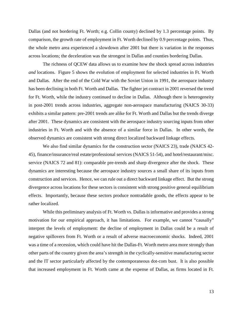
The richness of QCEW data allows us to examine how the shock spread across industries

and locations. Figure 5 shows the evolution of employment for selected industries in Ft. Worth

and Dallas. After the end of the Cold War with the Soviet Union in 1991, the aerospace industry

has been declining in both Ft. Worth and Dallas. The fighter jet contract in 2001 reversed the trend

for Ft. Worth, while the industry continued to decline in Dallas. Although there is heterogeneity

in post-2001 trends across industries, aggregate non-aerospace manufacturing (NAICS 30-33)

exhibits a similar pattern: pre-2001 trends are alike for Ft. Worth and Dallas but the trends diverge

after 2001. These dynamics are consistent with the aerospace industry sourcing inputs from other

industries in Ft. Worth and with the absence of a similar force in Dallas. In other words, the

observed dynamics are consistent with strong direct localized backward linkage effects.

We also find similar dynamics for the construction sector (NAICS 23), trade (NAICS 42-

45), finance/insurance/real estate/professional services (NAICS 51-54), and hotel/restaurant/misc.

service (NAICS 72 and 81): comparable pre-trends and sharp divergence after the shock. These

dynamics are interesting because the aerospace industry sources a small share of its inputs from

construction and services. Hence, we can rule out a direct backward linkage effect. But the strong

divergence across locations for these sectors is consistent with strong positive general equilibrium

effects. Importantly, because these sectors produce nontradable goods, the effects appear to be

rather localized.

While this preliminary analysis of Ft. Worth vs. Dallas is informative and provides a strong

motivation for our empirical approach, it has limitations. For example, we cannot “causally”

interpret the levels of employment: the decline of employment in Dallas could be a result of

negative spillovers from Ft. Worth or a result of adverse macroeconomic shocks. Indeed, 2001

was a time of a recession, which could have hit the Dallas-Ft. Worth metro area more strongly than

other parts of the country given the area’s strength in the cyclically-sensitive manufacturing sector

and the IT sector particularly affected by the contemporaneous dot-com bust. It is also possible

that increased employment in Ft. Worth came at the expense of Dallas, as firms located in Ft.

14

Worth could poach workers from firms located in Dallas. Hence, we need to explore employment

dynamics of other cities similar to Dallas/Ft. Worth to get a sense of the “aggregate” effect.

To this end, we plot employment and DOD spending time series for Houston and San

Antonio, two large cities in other regions of Texas. The figure demonstrates that the Dallas-Ft.

Worth metro area received much more in military contract funding than either Houston or San

Antonio. At the same time, there is no apparent divergence in employment across the metro areas.

One interpretation of this result is that spillover effects are very strong (that is, the Dallas-Ft. Worth

area lifted Houston and San Antonio) and this is why all three metropolitan areas comoved.

Alternatively, aggregate employment multipliers for government spending could be small. That

is, there was simply a reallocation of jobs from Dallas to Ft. Worth. But it is also possible that

neither Houston nor San Antonio are good cities to serve as a control group. There could be

potentially confounding factors that attenuate differences and result in understated multipliers. For

example, Houston benefited from the post-2001 era of high oil prices while San Antonio could

have grown faster because it was a smaller city. In this case, Dallas-Ft.Worth would have declined

without the shock and the comovement with Houston and San Antonio could be consistent with

strong localized multipliers.

This case study highlights that DOD spending shocks have positive multipliers but the

effects are heterogeneous across space and industries. We observe that places proximate to the

location with the shock tend to do better than more distance places. Industries connected to the

“shocked” industry likely experience stronger growth via backward linkages and other industries

can grow faster via general equilibrium effects. It is also clear that finding a proper control group

for large cities is challenging, making a more systematic econometric methodology necessary. We

thus move on to describe our approach to taking advantage of this rich source of spending variation

and outcomes.

5. Empirical Specification and Methodology

Our baseline econometric specification builds on the approach in Auerbach and Gorodnichenko

(2013) and Nakamura and Steinsson (2014). In particular, we start with the following specification

𝑌𝑌ℓ,𝑡𝑡+ℎ − 𝑌𝑌ℓ,𝑡𝑡−1

𝑌𝑌ℓ,𝑡𝑡−1= 𝛽𝛽

𝐺𝐺ℓ,𝑡𝑡+ℎ − 𝐺𝐺ℓ,𝑡𝑡−1

𝑌𝑌ℓ,𝑡𝑡−1+ 𝛼𝛼ℓ + 𝜆𝜆𝑡𝑡 + 𝜖𝜖ℓ𝑡𝑡, (1)

15

where ℓ, t and ℎ index locations (cities), time, and horizon, 𝑌𝑌 is an outcome variable (output,

employment, etc.), G is military spending, and 𝛼𝛼ℓ and 𝜆𝜆𝑡𝑡 are location and time fixed effects.

Normalization of government spending changes will vary depending on the outcome variable. The

coefficient of interest, 𝛽𝛽, represents the local DOD spending multiplier: the dollar amount of output

produced by a dollar of local DOD spending.

We augment specification (1) in several dimensions. First, we examine spillover effects

of aggregate government spending in one location on aggregate outcomes in other locations.

Second, we consider local and spillover outcomes across industries as well. In this most detailed

analysis, the augmented specification is

𝑌𝑌𝑖𝑖,ℓ,𝑡𝑡+ℎ − 𝑌𝑌𝑖𝑖,ℓ,𝑡𝑡−1

𝑌𝑌𝑖𝑖,ℓ,𝑡𝑡−1= 𝛽𝛽

𝐺𝐺𝑖𝑖,ℓ,𝑡𝑡+ℎ − 𝐺𝐺𝑖𝑖,ℓ,𝑡𝑡−1

𝑌𝑌𝑖𝑖,ℓ,𝑡𝑡−1+ 𝛾𝛾

𝐺𝐺�𝑖𝑖,ℓ,𝑡𝑡+ℎ − 𝐺𝐺�𝑖𝑖,ℓ,𝑡𝑡−1

𝑌𝑌𝑖𝑖,ℓ,𝑡𝑡−1+ 𝛼𝛼𝑖𝑖,ℓ + 𝜆𝜆𝑡𝑡 + 𝜖𝜖𝑖𝑖,ℓ,𝑡𝑡, (2)

where 𝑖𝑖 indexes industries, 𝐺𝐺�𝑖𝑖,ℓ,𝑡𝑡 is a measure of spending in other industries/locations, and 𝛼𝛼𝑖𝑖,ℓ is

the industry×location fixed effect.

To quantify the size of spillovers, we construct several measures of 𝐺𝐺�𝑖𝑖,ℓ,𝑡𝑡. First, when we

examine cross-industry spillovers in a given location, we consider two measures of 𝐺𝐺�𝑖𝑖,ℓ,𝑡𝑡:

𝐺𝐺�𝑖𝑖,ℓ,𝑡𝑡(1) = � 𝜔𝜔𝑗𝑗→𝑖𝑖 × 𝐺𝐺𝑗𝑗,ℓ,𝑡𝑡

𝑗𝑗

𝐺𝐺�𝑖𝑖,ℓ,𝑡𝑡(2) = � (1 − 𝜔𝜔𝑗𝑗→𝑖𝑖) × 𝐺𝐺𝑗𝑗,ℓ,𝑡𝑡

𝑗𝑗

where 𝜔𝜔𝑗𝑗→𝑖𝑖 is the direct input requirement of industry 𝑖𝑖 for industry 𝑗𝑗.9 𝐺𝐺�𝑖𝑖,ℓ,𝑡𝑡(1) captures direct

backward linkage effects, while 𝐺𝐺�𝑖𝑖,ℓ,𝑡𝑡(2) captures “general equilibrium” effects. Direct input

requirements come from BEA’s 2016 Input-Output tables (75 industries).

Second, when we investigate geographical spillovers, we consider:

𝐺𝐺�ℓ,𝑡𝑡(3) = � 𝑑𝑑(ℓ′, ℓ) × 𝐺𝐺ℓ′,𝑡𝑡

ℓ′

9 When we calculate 𝐺𝐺�𝑖𝑖,ℓ,𝑡𝑡

(2) , we set 𝜔𝜔𝑖𝑖→𝑖𝑖 = 1 because we include 𝐺𝐺𝑖𝑖,ℓ,𝑡𝑡 as a separate regressor to isolate GE effects.

16

where 𝑑𝑑(ℓ′, ℓ) is a weight that depends on the distance between locations ℓ′ and ℓ. We explore

several functional forms for 𝑑𝑑(ℓ′,ℓ). For instance, we consider 𝑑𝑑(ℓ′, ℓ) = [𝑑𝑑𝑖𝑖𝑑𝑑𝑑𝑑𝑑𝑑𝑑𝑑𝑑𝑑𝑑𝑑(ℓ′,ℓ)]−1

and 𝑑𝑑(ℓ′,ℓ) = 1 if ℓ′ is the nearest-neighbor city to city ℓ and zero otherwise.

Third, when we analyze cross-industry/location spillovers, we utilize:

𝐺𝐺�𝑖𝑖,ℓ,𝑡𝑡(4) = � � 𝜔𝜔𝑗𝑗→𝑖𝑖 × 𝑑𝑑(ℓ′,ℓ) × 𝐺𝐺𝑗𝑗,ℓ′,𝑡𝑡

ℓ′𝑗𝑗

𝐺𝐺�𝑖𝑖,ℓ,𝑡𝑡(5) = � � (1 − 𝜔𝜔𝑗𝑗→𝑖𝑖) × 𝑑𝑑(ℓ′, ℓ) × 𝐺𝐺𝑗𝑗,ℓ′,𝑡𝑡

ℓ′𝑗𝑗

where 𝐺𝐺�𝑖𝑖,ℓ,𝑡𝑡(4) and 𝐺𝐺�𝑖𝑖,ℓ,𝑡𝑡

(5) have the same “backward linkage” and “general equilibrium” interpretations

as those for the local industry spillovers 𝐺𝐺�𝑖𝑖,ℓ,𝑡𝑡(1) and 𝐺𝐺�𝑖𝑖,ℓ,𝑡𝑡

(2) .

Nakamura and Steinsson (2014) estimate specification (1) and its variants using an

instrumental variable (IV) approach where the instrument is constructed as in Bartik (1994). That

is, 𝐺𝐺ℓ,𝑡𝑡+ℎ−𝐺𝐺ℓ,𝑡𝑡−1𝑌𝑌ℓ,𝑡𝑡−1

is instrumented with 𝑠𝑠ℓ×(𝐺𝐺𝑡𝑡+ℎ−𝐺𝐺𝑡𝑡−1)𝑌𝑌ℓ,𝑡𝑡−1

where 𝐺𝐺𝑡𝑡 is aggregate government spending

and 𝑑𝑑ℓ is the average share of location ℓ in total government spending over a relevant time period.

Nakamura and Steinsson (2014) use this instrument to address potential endogeneity of

government spending due to political factors in determining military spending and measurement

error. While these sources of endogeneity are certainly possible in our more disaggregate setting,

we use the Bartik instrument chiefly for another reason.

We are interested in the effects of government spending – that is, new goods and services

provided by contractors to the government. Many contracts, however, represent not only payment

for new production but also payment for production that would have occurred anyway, either

because the specific contract was anticipated or because firms smooth production over lumpy

contracts. For example, assume that Boeing correctly forecasts the average airplane orders over

the next three years. The timing of a contract simply represents the moment they receive cash (or

promises of future cash payments) but does not correspond to actual new production. For Boeing,

the contract represents a “wealth transfer” rather than an exchange for a new service.10 Such a

contract should have little or no effect on income/employment/production.

10 The term “wealth transfer” here is the government-to-firm analog of the county-to-country use of the term in the international context (e.g., Gourinchas, Rey, and Truempler 2012). An alternative term with similar meaning is “non-

17

More formally, consider Δ𝐺𝐺ℓ,𝑡𝑡 ≡ 𝐺𝐺ℓ,𝑡𝑡 − 𝐺𝐺ℓ,𝑡𝑡−1 = Δ𝐺𝐺ℓ,𝑡𝑡𝑊𝑊 + Δ𝐺𝐺ℓ,𝑡𝑡

𝑃𝑃 , where Δ𝐺𝐺ℓ,𝑡𝑡𝑊𝑊 is a “wealth”

transfer (i.e., the “timing” component in the Auerbach and Gorodnichenko (2016) classification)

and Δ𝐺𝐺ℓ,𝑡𝑡𝑃𝑃 induces new production (i.e., the “level” and “identity” components). By mixing Δ𝐺𝐺ℓ,𝑡𝑡

𝑊𝑊

and Δ𝐺𝐺ℓ,𝑡𝑡𝑃𝑃 , we are likely to have a downward bias in the size of the multiplier to government

spending shocks. One strategy to remove this bias is to use information about contracts to

narratively separate Δ𝐺𝐺ℓ,𝑡𝑡𝑊𝑊 and Δ𝐺𝐺ℓ,𝑡𝑡

𝑃𝑃 , which is a big task given the sheer volume and heterogeneity

of contracts. Another strategy is to find a variable that is correlated with Δ𝐺𝐺ℓ,𝑡𝑡𝑃𝑃 and uncorrelated

with Δ𝐺𝐺ℓ,𝑡𝑡𝑊𝑊 and use this variable as an instrument for Δ𝐺𝐺ℓ,𝑡𝑡.

The Bartik instrument effectively provides such a filter: aggregate DOD spending

represents new production of goods and services and thus 𝑠𝑠ℓ×(𝐺𝐺𝑡𝑡+ℎ−𝐺𝐺𝑡𝑡−1)𝑌𝑌ℓ,𝑡𝑡−1

picks up only spending-

related changes in 𝐺𝐺ℓ,𝑡𝑡+ℎ−𝐺𝐺ℓ,𝑡𝑡−1𝑌𝑌ℓ,𝑡𝑡−1

and filters out the wealth transfers (including anticipated contracts).

In other words, the Bartik instrument helps us to isolate the component of contracts that

corresponds to new production by relating location-specific contracts to changes in aggregate

production/spending. Figure 1 demonstrates that national DOD spending changes correspond to

changes in new production of goods and services as measured by the NIPA. As to the geography

variation that the instrument provides, Table 2 shows the average shares of defense spending for

the cities that receive the largest shares of military spending, in absolute terms and as a share of

local income. Intuitively, 𝐺𝐺𝑡𝑡 is largely driven by “level” shocks while 𝑑𝑑ℓ captures the “identity”

component. In summary, the Bartik instrument is the predicted change in local spending based on

changes in national spending and therefore isolates new production from wealth transfers.

An alternative to using a Bartik instrument is to examine local spending changes over

longer time horizons. Persistent long-term changes in government spending are more likely to

represent new orders for goods and services than are temporary or short-term changes. Consider

again the Boeing example. A six-year increase in contract allocations will likely induce additional

production over that time period, while a quarterly increase could easily be offset by decrease in

contracts in subsequent quarters, which Boeing likely anticipates and smooths production over.

flow adjustments” (Obstfeld 2012). More generally, we use the term to refer to any exchange or transfer of assets that is not associated with additional production.

18

An advantage of the Bartik approach over using long-horizon spending changes is that Bartik

approach preserves a longer time series dimension of the data.

It is straightforward to tailor this instrument to specification (2). Specifically, 𝐺𝐺𝑖𝑖,ℓ,𝑡𝑡+ℎ−𝐺𝐺𝑖𝑖,ℓ,𝑡𝑡−1

𝑌𝑌𝑖𝑖,ℓ,𝑡𝑡−1 is instrumented with 𝑠𝑠𝑖𝑖,ℓ×(𝐺𝐺𝑡𝑡+ℎ−𝐺𝐺𝑡𝑡−1)

𝑌𝑌ℓ,𝑡𝑡−1 where 𝑑𝑑𝑖𝑖,ℓ is the average share of industry 𝑖𝑖

location ℓ in total government spending. In a similar spirit, 𝐺𝐺�𝑖𝑖,ℓ,𝑡𝑡+ℎ−𝐺𝐺�𝑖𝑖,ℓ,𝑡𝑡−1

𝑌𝑌𝑖𝑖,ℓ,𝑡𝑡−1 is instrumented with

�̃�𝑠𝑖𝑖,ℓ×(𝐺𝐺𝑡𝑡+ℎ−𝐺𝐺𝑡𝑡−1)𝑌𝑌ℓ,𝑡𝑡−1

where �̃�𝑑𝑖𝑖,ℓ is heuristically the average share of aggregate government spending in

industries/locations, appropriately weighted, e.g., by (1 − 𝜔𝜔𝑗𝑗→𝑖𝑖) and 𝑑𝑑(ℓ′, ℓ)) that are connected

to industry 𝑖𝑖 in location ℓ.

Note that because the error term in specifications (1) and (2) is likely to be correlated across

industries and locations, we cluster standard errors by state. We experimented with alternative

approaches to compute sampling uncertainty in the estimated multipliers and found that clustering

by state provides conservative standard errors.

6. Effects of Local Defense Spending

We now present our results, examining the effects of defense spending on city-level total and

industry-level output and on neighboring regions’ output, in the aggregate and by industry. To

build a perspective, we start with the analysis of local multipliers and then investigate spillover

effects. Our baseline specification employs the instrumental variable approach described in the

previous section.

A. Employment, Earnings, and GDP Multipliers

In a first pass at the data, we use specification (1) to estimate fiscal multipliers at the city level for

employment, earnings and GDP. Using our instrumental variable approach, we find (Panel B,

Table 3) that an increase in DOD spending by a percent of local earnings causes local employment

to increase by 0.19 percent11 and earnings to increase by 0.32 percent on impact. And while

11 To estimate responses of employment to military spending shocks, we use percent change of employment growth as the dependent variable in specification (1) and change in military spending normalized by earnings as the regressor in specification (1).

19

earnings for workers (both new hires and incumbents) increase by 32 cents for every dollar of

DOD spending, total value added in the city increases by roughly a dollar. The estimates are

similar whether based on one-year multipliers or the multiplier effects of longer-horizon changes

in DOD spending on long-horizon output (rows labeled 2-year multiplier and 4-year multiplier).

Note that these estimates (and all other estimates in the tables) are based on (instrumented) changes

in DOD spending through horizon ℎ (0 or 2 or 4 in the table), so the denominator for the multiplier

estimates includes changes in DOD spending over the full horizon.12 Given the stability of

estimates across different horizons, we will focus on one-year (“impact”) multipliers in the

remainder of the paper. We also observe that the instruments are generally strong with the first-

stage F-statistic being comfortably well above 10.

To put these figures in context, the employee compensation share of each dollar of

industry-level output is approximately $0.30 (based on averages over industries of compensation

shares provided in the BEA input-output tables). The remainder is allocated to intermediate inputs

($0.50) and gross operating surplus ($0.20). Therefore, in the absence of any spillovers or general

equilibrium effects, one would expect a highly localized value-added (GDP) multiplier of

approximately $0.50. The fact that the point estimate of the city-level multiplier exceeds unity

implies potentially substantial within-location positive spillovers. The city-level GDP multiplier

is smaller than state-level estimates (e.g., Nakamura and Steinsson), which is suggestive of positive

geographic spillovers as well.

The OLS estimates (Panel A) are uniformly lower than the IV estimates, potentially

reflecting endogeneity of government spending but also potentially demonstrating the importance

of the Bartik instrument in capturing the component of local contracts that corresponds to ramp-

ups and ramp-downs in actual spending. Consistent with the notion that longer-horizon spending

changes contain a larger share of actual production increases (rather than wealth transfers), the

OLS coefficients are increasing with the time horizon.

We view these results as largely consistent with the results reported in previous studies.

For example, our estimates imply that $100,000 in Department of Defense contracts generates 0.84

(s.e. 0.24) year-jobs. This magnitude is in line with Chodorow-Reich (2018) reporting a range

12 Recall that we distribute outlays over the length of contracts, so that, even if a locality receives only one contract during a period of several quarters or years, there will typically be a change in measured spending over several periods after the initial contract date.

20

from 0.76 to 3.80 year-jobs estimated on variation due to the 2009 American Recovery and

Reinvestment Act (ARRA). While comparing these figures, one should bear in mind that our

sample covers many years of economic expansion in the United States and that the ARRA

spending happened during one of the worst recessions which, according to the logic in Auerbach

and Gorodnichenko (2012), likely resulted in higher job growth per a given amount of government

spending during the period when ARRA was implemented. The size of the GDP multiplier is also

broadly in agreement with estimates provided in earlier studies, although our estimate tends to be

on the lower side of the available estimates which are typically close to 1.5. However, it should

be kept in mind that, in estimating city-level GDP multipliers, we are not yet incorporating the

spillover effects in nearby locations, which, as reported below, increase estimated multipliers over

larger geographical areas consistent with those used in other studies.

B. Geographic Spillovers

How does DOD spending spill out geographically to neighboring cities? We address this question

first by examining fiscal effects across cities within states.13 To determine the effect of spending

on output in surrounding cities, we estimate “outflow” effects:

𝑌𝑌�ℓ,𝑡𝑡 − 𝑌𝑌�ℓ,𝑡𝑡−1

𝑌𝑌�ℓ,𝑡𝑡−1= 𝛽𝛽𝑜𝑜𝑜𝑜𝑡𝑡

𝐺𝐺ℓ,𝑡𝑡 − 𝐺𝐺ℓ,𝑡𝑡−1

𝑌𝑌�ℓ,𝑡𝑡−1+ 𝛼𝛼ℓ + 𝜆𝜆𝑡𝑡 + 𝜖𝜖ℓ,𝑡𝑡 (3)

where 𝑌𝑌�ℓ,𝑡𝑡 is output in other cities in the same state as city 𝑙𝑙. We find that a dollar of spending in

a city increases earnings and GDP in other cities in the state (the “outflow” effect) by between

$0.42 and $0.60 (Table 4, columns 3 and 4); that is, the outflow effect is between a half and a

whole of the within-city effect. Combining the local and outflow effects of DOD spending on

GDP (1.05 plus 0.42) yields a total within-state effect of approximately 1.5, which is similar to

state-level multiplier estimates from the literature (see, e.g., Nakamura and Steinsson (2014) for

DOD spending effects and Chodorow-Reich (2018) for a metastudy of state-level effects of other

forms of fiscal stimulus). Therefore, net effects on nearby localities are quite substantial.

13 While we consider neighboring cities only within states, our findings that the magnitude of spillovers decline sharply with distance suggests that extending the analysis to include cross-state spillovers would have little impact on the pattern.

21

Of course, these benefits are spread out across localities, and the outflow effect may be

uninformative to residents of a locality that are interested in how they will be affected by spending

elsewhere in the state. To this end, we also estimate what we refer to as “inflow” effects: the effect

of a dollar of spending in other cities in the state on an observed city:

𝑌𝑌ℓ,𝑡𝑡 − 𝑌𝑌ℓ,𝑡𝑡−1

𝑌𝑌ℓ,𝑡𝑡−1= 𝛾𝛾𝑖𝑖𝑖𝑖

𝐺𝐺�ℓ,𝑡𝑡 − 𝐺𝐺�ℓ,𝑡𝑡−1

𝑌𝑌ℓ,𝑡𝑡−1+ 𝛼𝛼ℓ + 𝜆𝜆𝑡𝑡 + 𝜖𝜖ℓ,𝑡𝑡. (4)

Table 4 (columns 1 and 2) suggests that inflow effects are meaningful but not particularly large,

with larger point estimates of inflow effects on GDP (0.020) than point estimates of inflow effects

on earnings (0.007).14

To what extent do spillover effects depend on distance? To address this question, for each

city in our sample and for different distance categories (less than 50 miles, between 50 and 100

miles, etc.) we identify a “neighbor” city that is of roughly equal size (within 10 percent) and,

more specifically, the closest to the city in terms of size and distance within that distance category.

We then estimate how spending in the observation city affects earnings in neighbor cities. A

neighbor city within 50 miles of the source city receives a substantial benefit of approximately half

of the benefit of the home city (a multiplier of 0.136 in column 2 of Table 5 compared to a

multiplier of 0.306 in column 1 of Table 5). These spillover effects dissipate rather rapidly. Point

estimates of multipliers reach zero for neighbors that are over 50 miles from the source city

(columns 3, 4 and 5).15

These estimates suggest that DOD spending positively affects nearby locations,

particularly those that are closest in proximity. There is no evidence that DOD spending in a city

systematically reduces output in other localities. This finding is consistent with extant evidence

of positive fiscal spillovers across geographies (e.g., Dupor and McCrory 2018) and motivates an

exploration of cross-industry spillovers to determine whether there are any local crowding-out

effects of DOD spending.

14 Note that there is no necessary relationship between the sizes of estimated inflow and outflow effects. For example, if spending shocks occur in a small number of cities, the average outflow effect of these shocks may be large but the inflow effects for the typical city may be small. This may be especially true if spillovers occur over a very small geographic area, affecting only a small number of other locations. 15 The number of observations in each sample varies based on the number of identifiable neighbor cities for each distance category.

22

C. Multipliers by Size and Gravity

The positive estimates of geographic spillovers suggest that fiscal multipliers are increasing in the

size of the geographical unit of observation. Consistent with this notion, Demyanyk et al. (2018)

find that city-level multipliers16 are larger than county-level multipliers (and smaller than estimates

of state-level multipliers from the literature). Here we directly examine how fiscal multipliers vary

with city size. To do so, we assign size based on cities’ average income over the sample. The size

distribution is heavily right-tailed (skewness is 8.5), reflecting a small number (approximately

10%) of exceptionally large cities with size between 10 and 300 times the median size.17

We find that among cities in the mass of the distribution, there is little detectable

relationship between city size and fiscal multipliers. However, cities at the upper end of the size

distribution have much larger multipliers than other cities (Table 6). The estimated multiplier for

cities in the top decile of the distribution is 0.75 (column 2), and the multiplier for cities in the top

5% of the distribution is 1.35 (column 3).18

D. Industry Spillovers and Crowding Out

To what extent does local industry-level spending affect output, both for industries that receive the

spending and for other local industries? To address this question we turn to city-industry-level

16 Recall that cities encompass metropolitan areas, not simply the central cities themselves. 17 Median income of cities in the bottom decile of the size distribution is roughly 1/4 of median income for the sample, while median income of cities in the top size decile is 21 times the sample median. 18 The evidence of positive spillovers and size-dependent multipliers implies that locations benefit from proximity to locations that receive DOD spending. An open question is whether the inverse is true. Does a recipient city benefit from proximity to other cities? In other words, are multipliers higher in cities that are isolated or in cities surrounded by economic activity? Proximity could be expected to lead to higher or lower multipliers. Subcontractors in nearby cities may compete with subcontractors in locations that receive the DOD spending, thereby dampening local income effects. But nearby cities may also provide necessary inputs into production of local contractors, especially when recipient locations do not produce such inputs locally. Nearby cities may also increase local multipliers through consumption effects, with DOD spending in a recipient location inducing higher spending in a nearby city, which may have a second-round positive effect on the recipient location. To explore the effects of proximity, we derived a city-specific measure of nearby economic activity by summing income (discounted by distance) across other cities. We found that, conditional on city size, multipliers appear to be slightly larger in the presence of nearby economic activity. We conjecture that a more detailed exploration of this issue would be a fruitful avenue for future research.

23

data on spending and income. To disentangle direct effect from spillover effects, we create three

measures of DOD spending.

The first measure is direct spending from the DOD on goods produced by an industry. This

measure yields an estimate of the value added by the local industry’s workers (if using the earnings

measure) and capital (when examining GDP). Estimates of multipliers from this measure are

comparable to the impact multipliers in Table 3, the differences being due to the use of industry-

city observations rather than city observations aggregated across industries.

The second measure is indirect DOD spending on that industry based on input requirements

of other industries in that location that receive DOD spending (i.e., measure 𝐺𝐺�𝑖𝑖,ℓ,𝑡𝑡(1) ). This measure

yields an estimate of the local sourcing for DOD contracts and is analogous to estimates of

backward linkages previously explored in the context of foreign direct investment (e.g.,

Gorodnichenko, Svejnar, and Terrell 2014). An estimate of zero would imply that industries

source intermediate inputs almost exclusively from other locations, as would be expected in a

world with no trade costs, while positive estimates signal the importance of local sourcing.

The third measure is total DOD spending in other industries, net of input requirements for

the observed industry (i.e., measure 𝐺𝐺�𝑖𝑖,ℓ,𝑡𝑡(2) ). This measure yields an estimate of what we interpret

as general equilibrium effects, which include indirect effects such as reallocation of production

factors or positive demand externalities other than through direct backward linkages.19

We report results in Table 7 for labor income and GDP. All estimates are for one-year (i.e.,

impact) multipliers. Direct effects of industry-level spending are strong (columns 1 and 5 of Table

7) yet slightly lower than city-level effects (Table 3), consistent with positive spillovers across

industries within a city. Columns 2 and 6 yield direct estimates of spillovers through intermediate

input backward linkages. These estimates are of similar magnitudes to the direct effect, indicating

strong local sourcing. The large positive estimate indicates that local backward linkages is an

important source of positive across-industry spillovers.

While backward linkages are by definition associated with non-negative spillovers,

production in one industry can have negative effects on other industries through general

19 Although there is no obvious scaling to use in computing general equilibrium effects, this lack of scaling for the variable should be kept in mind when comparing the coefficients for this spillover effect and the one based on backward production linkages. A one-dollar shock to the production linkage variable would have a one-dollar spillover if the affected industry satisfies all of the increased input demand of the shocked industry. But a one-dollar shock’s effect on other industries simply depends on the shock’s overall general equilibrium effects.

24

equilibrium effects, including through the reallocation of local factors of production. The third

spending measure, spending in other industries net of backward linkages, allows us to estimate the

sign and magnitude of these general equilibrium effects. The results indicate (column 3) that such

effects are on average positive for income (perhaps operating through income multipliers) although

small in magnitude. The GDP estimates (column 7), which are based on far fewer observations

(given the limited coverage of city-level GDP data), are too noisy to detect general equilibrium

effects. Overall, we find no evidence of DOD spending crowding out non-recipient industries.

Rather, we detect crowding in of earnings, both through input linkages and through general

equilibrium effects.

E. Industry/Geography Spillovers

As a final attempt to uncover effects of crowding out or crowding in, we examine industry-level

spillover effects across locations, combining the two spillover dimensions already considered. To

do so, we construct a summary measure of industry-level spending in nearby cities within a

specified distance from the observation city. Specifically, for each city, we examine total industry-

level spending within a 50-mile radius, between 50 and 100 miles, and between 100 and 150 miles

respectively. Using the industry-level measures of nearby spending, we then construct measures

of backward linkages (i.e., measure 𝐺𝐺�𝑖𝑖,ℓ,𝑡𝑡(4) ) and spending in other industries net backward linkages

(i.e., measure 𝐺𝐺�𝑖𝑖,ℓ,𝑡𝑡(5) ) in the same manner as we did for the within-city industry-level analysis.

First consider the direct effects of nearby same-industry spending (column 1 of Table 8).

One would a priori expect such spending to be the most likely avenue for crowding out, since

factors of production are likely strong substitutes across short distances within industries. We find

that the effects of nearby spending on same-industry local income is generally positive, although

small as expected.20

Spending in other nearby industries that is associated with backward linkages also has

positive local effects. Consistent with the presence of transportation costs, these effects dissipate

with distance (estimates fall from Panel A to Panel B to Panel C in column 2 of Table 8). The

GDP estimates are too noisy (on account of far fewer data points) to identify precise effects.

20 The only evidence of negative spillovers is in the effect of spending 100 to 150 miles away on local same-industry GDP (column 5, Panel B).

25

Finally, general equilibrium effects appear to be positive if anything. Nearby spending in

other unrelated industries positively affects a local industry (columns 3 and 7 of Table 8). In general,

these effects also dissipate with distance, consistent with the presence of transportation costs.

To summarize the industry-level evidence, we find that DOD spending in an industry in a

location exhibits positive spillovers to other industries in that location. These spillovers include

both demand for intermediate inputs (backward linkages) and general equilibrium spillovers such

as through income multipliers. There is no evidence of a net crowding out of other local industries.

That is, we do not find support for the hypothesis in Cohen, Coval, and Malloy (2011) that

government spending crowds out local employment. Even when we isolate the component of

spending that has no direct benefits to other local industries, we detect crowding-in rather than

crowding-out of employment in other local industries.

Turning to industry-level income in other locations, we again find little evidence that local

spending in an industry crowds out production, either in the same industry in nearby locations or

in other industries. Both the same industry and other industries in nearby locations appear to

benefit, although these benefits are small in magnitude. The same-industry year-on-year benefits

are potentially due to agglomeration effects, which are typically assumed to operate over longer

time horizons. The benefits across industries across space are due to backward linkages and

general equilibrium effects that are likely similar to the forces that benefit other industries in the

same location.21

21 Our body of evidence suggests that the economy features slack (and hence private activity is not crowded out by public purchases) on average over the business cycle. A natural follow-up question is whether multipliers are higher during periods of higher slack. Even if multipliers are slack-dependent, detecting this dependence in our setting is challenging due to the fact that slack is endogenous to government spending, especially at the annual frequency: if government spending is effective, then measured slack is low. The literature using subnational variation generally finds state-dependent multiplies although there is variation across studies (see Chodorow-Reich, 2018). Consistent with this literature, we found that multipliers are substantially higher for cities experiencing unemployment above the 25th percentile level. We did not find evidence that the strength of multipliers increases much as slack increases beyond the 25th percentile (Appendix Table 1). One interpretation of these results is that multipliers are high when there is some slack, but beyond that the amount of slack doesn’t matter (perhaps short-run aggregate supply curves are relatively flat and rapidly steepen only as the economy approaches capacity). The fact that the threshold level of unemployment is around the 25th percentile suggests that multipliers on average are high and don’t lead to crowding out. This is consistent with our industry-level results that, on average (across the business cycle) there is no systematic evidence of crowding out.

26

7. Interpretation and Concluding Remarks

In this paper, we have estimated local fiscal multipliers and spillovers for the United States using

a rich dataset based on U.S. Department of Defense contracts and a variety of outcome variables

relating to income and employment. Such data are especially useful for estimating the effects of

fiscal policy, because defense spending is a large component of government spending and likely

independent at the national level from short-run economic conditions. We use an instrumental

variable approach to address potential identification issues with respect to the timing.

Our evidence points to strong positive spillovers, both within and across locations. For

example, a dollar of government spending in a city increases income in neighboring cities by as

much as half of the extent to which it increases own-city income. These benefits, while large, appear

to dissipate fairly quickly with distance. By summing over within-city and rest-of-state effects, we

obtain a state-level multiplier of approximately 1.5. This estimate is similar in magnitude to prior

estimates of state-level multipliers (e.g., Nakamura and Steinsson 2014) but is obtained by estimating

the state-wide effect of a city-level shock rather than the effect of a state-wide shock.

A unique feature of our study is that, by examining demand shocks at the detailed industry-

location level, we are able to examine spillover channels as well as magnitudes. Both backward

linkages and general equilibrium effects (e.g., income multipliers) contribute to the positive

spillovers. We find no evidence that government spending in an industry/location crowds out

income in other local industries or in other locations. These findings are contrary to conventional

wisdom and the predictions of neoclassical theory. On the other hand, our evidence points to the

relevance of Keynesian-type models that feature excess capacity, either at the firm level or the

level of individual workers. These models even appear relevant for low-frequency (annual)

demand shocks, suggesting that excess capacity could be more than a temporary phenomenon.

Our evidence is corroborated by a number of indirect pieces of evidence. First, models of

excess capacity can explain the otherwise puzzling evidence that national government spending

shocks do not appear to cause interest rates to rise (Murphy and Walsh 2017). Second, our evidence

of positive general equilibrium effects is consistent with evidence that government spending either

increases consumption or does not decrease it in a meaningful way (e.g., Hall 2009). While some

models can explain rising consumption, they typically also predict rising interest rates in response

to government spending shocks (e.g., Leeper, Traum, and Walker 2017). Models of excess capacity

can simultaneously explain a negligible interest rate effect and rising consumption.

27

In addition to informing the strength of geographical spillovers, our evidence informs the

size of the closed-economy national multiplier. Channels through which national multipliers

decline relative to local multipliers include the reallocation of production factors, interest rate

channels, and negative wealth effects due to higher future taxes. We find no evidence that

employment falls in areas or industries that don’t directly receive the spending. This finding

suggests that interest rate channels and even tax channels are potentially weak. Therefore, our

evidence points to regional multipliers being lower bounds for national multipliers (see Chodorow-

Reich 2018 for further discussion).

Our study points to a number of directions for future research. As detailed data on defense

spending across countries becomes available, researchers can examine the relevance of national

borders on spillovers. Of particular interest would be an understanding of how spending by one

country increases income in neighboring countries and effects the spending country’s net asset

position. To what extent is the additional debt required for the spending offset by increased by

improvements in the current account through net exports to neighboring countries? Do the effects

depend on the size or wealth of the spending country, as predicted by models of excess capacity

and heterogeneous households/countries?22

In the meantime, the detailed U.S. Department of Defense data can inform us about a

number of relevant questions in macroeconomics. Do government spending shocks reduce excess

capacity at the firm-level? Or are firms hiring more workers or for longer hours? In other words,

does the excess capacity reside at the firm level (through labor hoarding, for example) or at the

worker level (in the form of unemployment or labor force nonparticipation)? Answers to these

questions are relevant for guiding estimates of potential output.

22 Murphy (2017), for example, predicts that in the presence of excess capacity, temporary spending shocks by a rich trading partner can have persistent and large effects on income for both the rich agent and its poorer trading partners.

28

References

Auerbach, Alan J., and Yuriy Gorodnichenko. 2012. “Measuring the Output Responses to Fiscal

Policy.” American Economic Journal: Economic Policy 4(2): 1-27.

Auerbach, Alan J., and Yuriy Gorodnichenko. 2013. “Output Spillovers from Fiscal Policy.”

American Economic Review 103(2): 141-146.

Auerbach, Alan J., and Yuriy Gorodnichenko. 2016. “"Effects of Fiscal Shocks in a Globalized

World.” IMF Economic Review 64 (1): 177-215.

Autor, David H., David Dorn, and Gordon H. Hanson. 2016. "The China Shock: Learning from

Labor-Market Adjustment to Large Changes in Trade," Annual Review of Economics 8(1):

205-240.

Bartik, Timothy. 1991. Who Benefits from State and Local Economic Development Policies? W.E.

Upjohn Institute.

Blanchard, Olivier, and Roberto Perotti. 2002. “An Empirical Characterization of the Dynamic

Effects of Changes in Government Spending and Taxes on Output.” Quarterly Journal of

Economics 117(4): 1329-1368.

Chodorow-Reich, Gabriel. 2018, forthcoming. “Geographic Cross-Sectional Fiscal Spending

Multipliers: What Have We Learned?” American Economic Journal: Economic Policy.

Clemens, Jeffrey and Stephen Miran. 2012. “Fiscal Policy Multipliers on Subnational Government

Spending.” American Economic Journal: Economic Policy 4(2): 46-68.

Cohen, Lauren, Joshua Coval, and Christopher Malloy. 2011, “Do Powerful Politicians Cause

Corporate Downsizing?” Journal of Political Economy 119(6): 1015-1060.

Demena, Binyam A., and Peter A. G. van Bergeijk. 2017. "A Meta-Analysis Of Fdi And

Productivity Spillovers In Developing Countries." Journal of Economic Surveys 31(2):

546-571.

Demyanyk, Yuliya, Elena Loutskina, and Daniel Murphy. 2018, forthcoming. “Fiscal Stimulus

and Consumer Debt.” Review of Economics and Statistics.

Dupor, Bill and Peter B. McCrory. 2018, forthcoming. “A Cup Runneth Over: Fiscal Policy

Spillovers from the 2009 Recovery Act.” Economic Journal.

Gourinchas, Pierre-Olivier, Helene Rey and Kai Truempler. 2012, "The Financial Crisis and The

Geography of Wealth Transfers," Journal of International Economics 88: 266-283.

29

Murphy, Daniel P. 2015. “How Can Government Spending Stimulate Consumption?” Review of

Economic Dynamics 18(3): 551–574.

Murphy, Daniel P. 2017. “Excess Capacity in a Fixed-Cost Economy.” European Economic

Review 91: 245–260.

Murphy, Daniel P. and Kieran Walsh. 2018. “Government Spending and Interest Rates.” Mimeo.

Nakamura, Emi, and Jón Steinsson. 2014. “Fiscal Stimulus in a Monetary Union: Evidence from

U.S. Regions.” American Economic Review 104(3): 753–792.

Obstfeld, Maurice. 2012. “Does the Current Account Still Matter?” American Economic Review

102(3): 1–23.

Smarzynska Javorcik, Beata. 2004. "Does Foreign Direct Investment Increase the Productivity of

Domestic Firms? In Search of Spillovers Through Backward Linkages." American

Economic Review 94(3): 605-627.

Suárez Serrato, Juan Carlos, and Philippe Wingender, 2016. "Estimating Local Fiscal Multipliers,"

NBER Working Paper 22425.

Blanchard, Olivier, Christopher J. Erceg, and Jesper Lindé, 2016. "Jump-Starting the Euro Area

Recovery: Would a Rise in Core Fiscal Spending Help the Periphery?," NBER

Macroeconomics Annual 2016, Volume 31, pages 103-182 National Bureau of Economic

Research, Inc.

Chodorow-Reich, Gabriel, Laura Feiveson, Zachary Liscow, and William Gui Woolston. 2012.

“Does State Fiscal Relief During Recessions Increase Employment? Evidence from the

American Recovery and Reinvestment Act.” American Economic Journal: Economic

Policy 4(3): 118-145.

Miyamoto, Wataru, Thuy Lan Nguyen, and Viacheslav Sheremirov, 2016. "The Effects of

Government Spending on Real Exchange Rates: Evidence from Military Spending Panel

Data." Working Papers 16-14, Federal Reserve Bank of Boston.

Ramey, Valerie A., 2011. "Identifying Government Spending Shocks: It's all in the Timing."

Quarterly Journal of Economics, 126(1): 1-50.

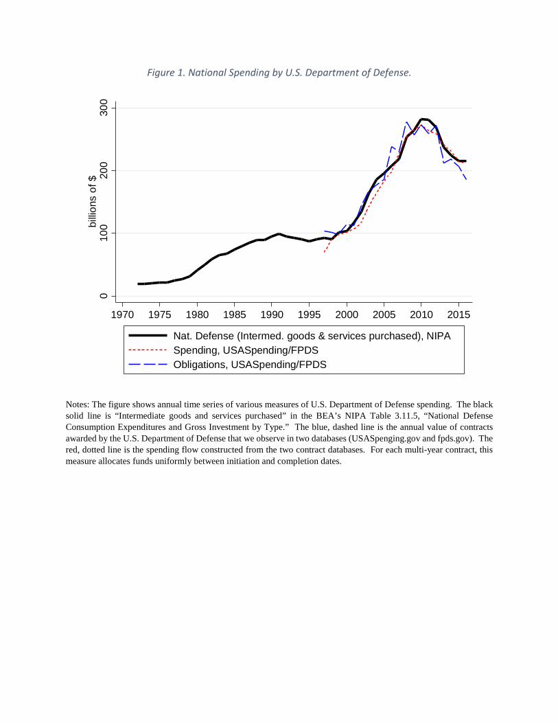
Figure 1. National Spending by U.S. Department of Defense.

Notes: The figure shows annual time series of various measures of U.S. Department of Defense spending. The black solid line is “Intermediate goods and services purchased” in the BEA’s NIPA Table 3.11.5, “National Defense Consumption Expenditures and Gross Investment by Type.” The blue, dashed line is the annual value of contracts awarded by the U.S. Department of Defense that we observe in two databases (USASpenging.gov and fpds.gov). The red, dotted line is the spending flow constructed from the two contract databases. For each multi-year contract, this measure allocates funds uniformly between initiation and completion dates.

010

020

030

0bi

llions

of $

1970 1975 1980 1985 1990 1995 2000 2005 2010 2015

Nat. Defense (Intermed. goods & services purchased), NIPASpending, USASpending/FPDSObligations, USASpending/FPDS

Figure 2. Map of the Fort Worth-Dallas Metropolitan Area.

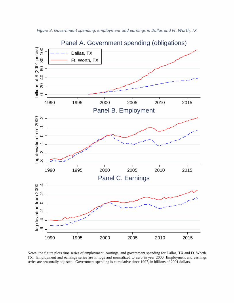
Figure 3. Government spending, employment and earnings in Dallas and Ft. Worth, TX.

Notes: the figure plots time series of employment, earnings, and government spending for Dallas, TX and Ft. Worth, TX. Employment and earnings series are in logs and normalized to zero in year 2000. Employment and earnings series are seasonally adjusted. Government spending is cumulative since 1997, in billions of 2001 dollars.

020

4060

8010

0bi

llions

of $

(200

1 pr

ices

)

1990 1995 2000 2005 2010 2015

Dallas, TXFt. Worth, TX

Panel A. Government spending (obligations)-.3

-.2-.1

0.1

.2lo

g de

viat

ion

from

200

0

1990 1995 2000 2005 2010 2015

Panel B. Employment

-.6-.4

-.20

.2.4

log

devi

atio

n fro

m 2

000

1990 1995 2000 2005 2010 2015

Panel C. Earnings

Figure 4. Local spillovers in the Dallas-Ft. Worth metropolitan area.

Notes: the figure plots time series of employment and government spending for Dallas, TX and Ft. Worth, TX as well as select counties around these two cities. Employment series are in logs, normalized to zero in year 2000. Employment series are seasonally adjusted. Government spending in billions of 2001 dollars is cumulative since 1997.

020

4060

8010

0ob

ligat

ions

, billi

ons

of $

(200

1 pr

ices

)

1990 1995 2000 2005 2010 2015

Dallas (1551)Tarrant/Ft. Worth (709)Denton (123)Ellis (33)Johnson (33)Hunt (24)Collin (181)

Panel A. Government spending (obligations)-1

-.50

.51

empl

oym

ent,

log

devi

atio

n fro

m 2

000

1990 1995 2000 2005 2010 2015

Panel B. Employment

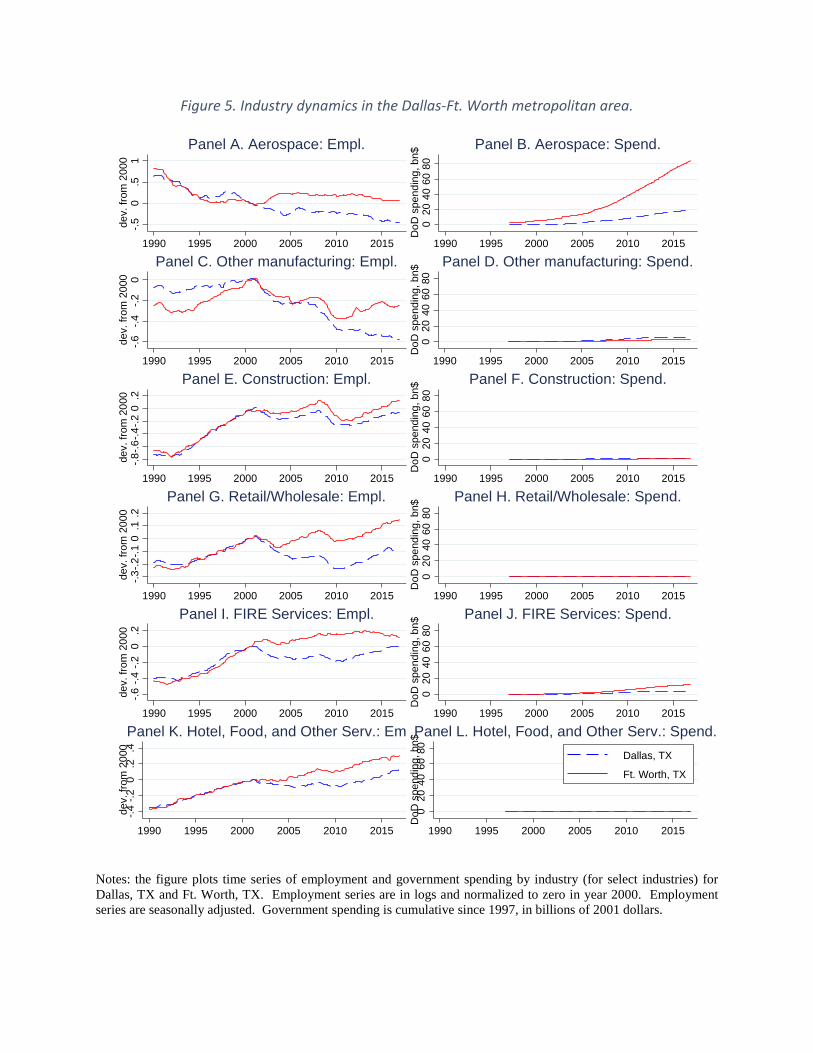
Figure 5. Industry dynamics in the Dallas-Ft. Worth metropolitan area.

Notes: the figure plots time series of employment and government spending by industry (for select industries) for Dallas, TX and Ft. Worth, TX. Employment series are in logs and normalized to zero in year 2000. Employment series are seasonally adjusted. Government spending is cumulative since 1997, in billions of 2001 dollars.

-.50

.51

dev.

from

200

0

1990 1995 2000 2005 2010 2015

Panel A. Aerospace: Empl.

020

4060

80D

oD s

pend

ing,

bn$

1990 1995 2000 2005 2010 2015

Panel B. Aerospace: Spend.-.6

-.4-.2

0de

v. fr

om 2

000

1990 1995 2000 2005 2010 2015

Panel C. Other manufacturing: Empl.

020

4060

80D

oD s

pend

ing,

bn$

1990 1995 2000 2005 2010 2015

Panel D. Other manufacturing: Spend.

-.8-.6

-.4-.2

0.2

dev.

from

200

0

1990 1995 2000 2005 2010 2015

Panel E. Construction: Empl.

020

4060

80D

oD s

pend

ing,

bn$

1990 1995 2000 2005 2010 2015

Panel F. Construction: Spend.

-.3-.2

-.10

.1.2

dev.

from

200

0

1990 1995 2000 2005 2010 2015

Panel G. Retail/Wholesale: Empl.

020

4060

80D

oD s

pend

ing,

bn$

1990 1995 2000 2005 2010 2015

Panel H. Retail/Wholesale: Spend.

-.6-.4

-.20

.2de

v. fr

om 2

000

1990 1995 2000 2005 2010 2015

Panel I. FIRE Services: Empl.

020

4060

80D

oD s

pend

ing,

bn$

1990 1995 2000 2005 2010 2015

Panel J. FIRE Services: Spend.

-.4-.2

0.2

.4de

v. fr

om 2

000

1990 1995 2000 2005 2010 2015

Panel K. Hotel, Food, and Other Serv.: Empl.

020

4060

80D

oD s

pend

ing,

bn$

1990 1995 2000 2005 2010 2015

Dallas, TX

Ft. Worth, TX

Panel L. Hotel, Food, and Other Serv.: Spend.

Figure 6. “Aggregate” effects of a government spending shock in Texas.

Notes: the figure plots time series of employment and government spending for three metropolitan areas. Employment and earnings series are in logs and normalized to zero in year 2000. Employment series are seasonally adjusted. Government spending is in billions of 2001 dollars, cumulative since 1997.

050

100

150

200

oblig

atio

ns, b

illion

s of

$ (2

001

pric

es)

1990 1995 2000 2005 2010 2015

Ft. Worth-Dallas, TXSan Antonio, TXHouston, TX

Panel A. Government spending (obligations)-.4

-.20

.2.4

empl

oym

ent,

log

devi

atio

n fro

m 2

000

1990 1995 2000 2005 2010 2015

Panel B. Employment

Table 1. Department of Defense contracts by industry.

BEA Industry Classification

Industry Spending per year, bn.

3364OT Aerospace and other transportation equipment 42.00 5412OP Miscellaneous professional, scientific, and technical services 36.07 334 Computer and electronic products 12.64 23 Construction 11.08 5415 Computer systems design and related services 7.49 42 Wholesale trade 5.72 524 Insurance carriers and related activities 5.71 332 Fabricated metal products 4.38 324 Petroleum and coal products 3.49 3361MV Motor vehicles, bodies and trailers, and parts 2.87 333 Machinery 2.59 481 Air transportation 1.91 81 Other services, except government 1.18 315AL Apparel and leather and allied products 1.17 311FT Food and beverage and tobacco products 1.15 325 Chemical products 1.07 335 Electrical equipment, appliances, and components 1.06 61 Educational services 0.95 483 Water transportation 0.93 51 Information 0.85

Notes: the table reports the volume of spending by the Department of Defense for selected industries (as defined by the Bureau of Economic Analysis (BEA). Spending is in billions of 2001 dollars. Spending is average over the 1997-2016 period. Industry 332 includes “Ammunition, arms, ordnance, and accessories manufacturing”.

Table 2. Average DOD Spending Shares by Cities.

CBSA/City

Share of National

DOD Spending

Spending as a Fraction of local income

Panel A: Cities with highest share of National DOD Spending Washington-Arlington-Alexandria, DC-VA-MD-WV 0.133 0.150 Dallas-Fort Worth-Arlington, TX 0.054 0.071 Los Angeles-Long Beach-Santa Ana, CA 0.052 0.040 Boston-Cambridge-Newton, MA-NH 0.041 0.055 Virginia Beach-Norfolk-Newport News, VA-NC 0.030 0.233 Philadelphia-Camden-Wilmington, PA-NJ-DE-MD 0.030 0.044 New York-Newark-Jersey City, NY-NJ-PA 0.028 0.019 Baltimore-Columbia-Towson, MD 0.027 0.087 San Diego-Carlsbad, CA 0.026 0.083 St. Louis, MO-IL 0.022 0.068 Phoenix-Mesa-Scottsdale, AZ 0.022 0.056

Panel B: Cities with highest DOD Spending Fraction of Income Lexington Park, MD 0.008 0.743 Fort Polk South, LA 0.001 0.596 Enterprise, AL 0.003 0.532 Fort Leonard Wood, MO 0.001 0.530 Norwich-New London, CT 0.016 0.489 Huntsville, AL 0.019 0.396 Camden, AR 0.001 0.386 Oshkosh-Neenah, WI 0.007 0.385 Hinesville, GA 0.001 0.366 Jacksonville, NC 0.002 0.350 Charleston-North Charleston, SC 0.004 0.342

Note: Cities defined as core-based statistical areas (CBSAs).

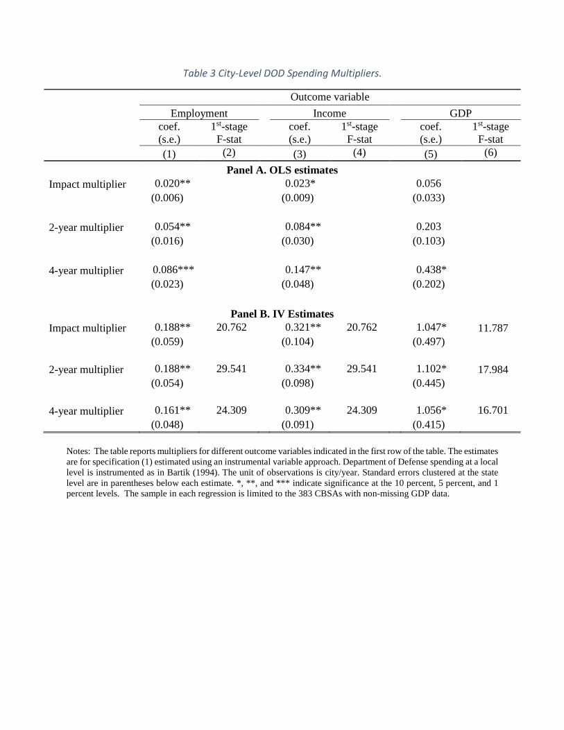
Table 3 City-Level DOD Spending Multipliers.

Outcome variable

Employment Income GDP

coef. (s.e.)

1st-stage F-stat

coef. (s.e.)

1st-stage F-stat

coef. (s.e.)

1st-stage F-stat

(1) (2) (3) (4) (5) (6) Panel A. OLS estimates

Impact multiplier 0.020** 0.023* 0.056 (0.006) (0.009) (0.033) 2-year multiplier 0.054** 0.084** 0.203 (0.016) (0.030) (0.103) 4-year multiplier 0.086*** 0.147** 0.438* (0.023) (0.048) (0.202)

Panel B. IV Estimates Impact multiplier 0.188** 20.762 0.321** 20.762 1.047* 11.787

(0.059) (0.104) (0.497)

2-year multiplier 0.188** 29.541 0.334** 29.541 1.102* 17.984 (0.054) (0.098) (0.445)

4-year multiplier 0.161** 24.309 0.309** 24.309 1.056* 16.701 (0.048) (0.091) (0.415)

Notes: The table reports multipliers for different outcome variables indicated in the first row of the table. The estimates are for specification (1) estimated using an instrumental variable approach. Department of Defense spending at a local level is instrumented as in Bartik (1994). The unit of observations is city/year. Standard errors clustered at the state level are in parentheses below each estimate. *, **, and *** indicate significance at the 10 percent, 5 percent, and 1 percent levels. The sample in each regression is limited to the 383 CBSAs with non-missing GDP data.

Table 4. Aggregate spillovers across locations.

Effects of spending in other cities in state on local city

(inflow effect)

Effect of spending in city on other cities in same state

(outflow effect) Earnings GDP Earnings GDP (1) (2) (3) (4)

One-year multiplier 0.007* 0.020* 0.424*** 0.600* (0.003) (0.009) (0.109) (0.225) N 5,595 5,610 5,590 5,530 1st-stage F-stat 98.88 113.18 33.15 25.86

Notes: Standard Errors clustered at the state level are in parentheses below each estimate. *, **, and *** indicate significance at the 10%, 5%, and 1% levels. The sample in each regression is limited to the 383 CBSAs with nonmissing GDP data.

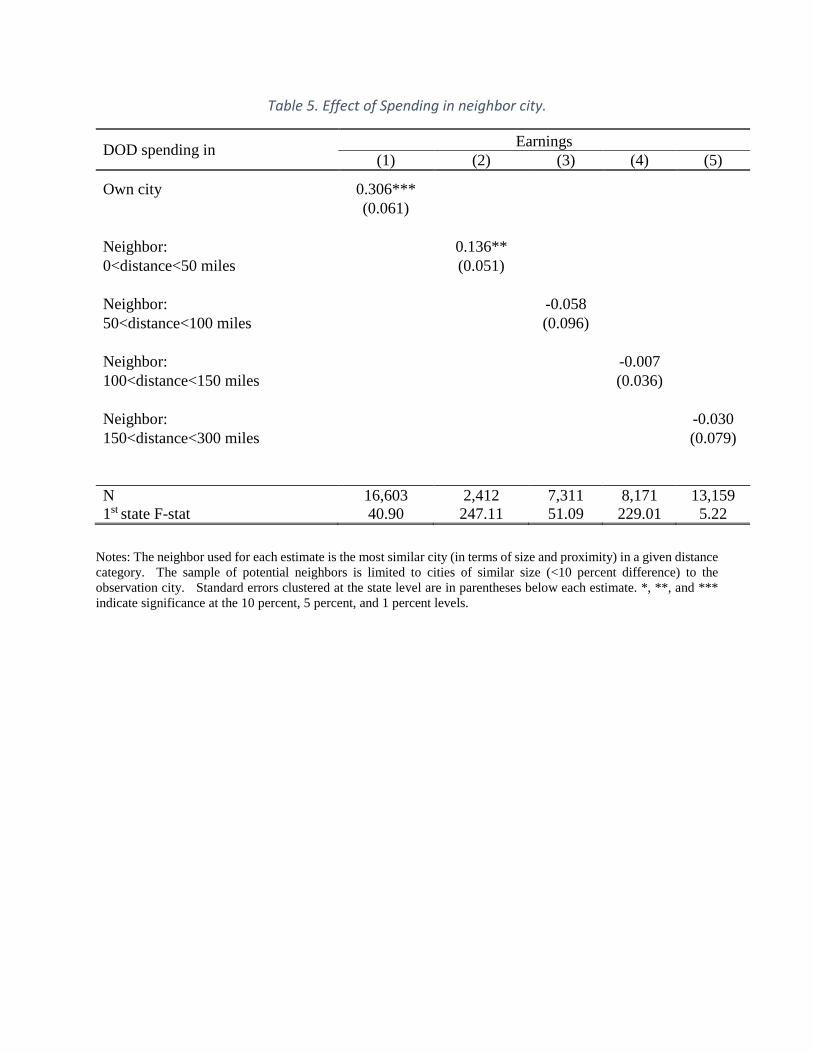
Table 5. Effect of Spending in neighbor city.

DOD spending in Earnings (1) (2) (3) (4) (5)

Own city 0.306*** (0.061)

Neighbor: 0.136** 0<distance<50 miles (0.051)

Neighbor: -0.058 50<distance<100 miles (0.096)

Neighbor: -0.007 100<distance<150 miles (0.036)

Neighbor: -0.030 150<distance<300 miles (0.079)

N 16,603 2,412 7,311 8,171 13,159 1st state F-stat 40.90 247.11 51.09 229.01 5.22

Notes: The neighbor used for each estimate is the most similar city (in terms of size and proximity) in a given distance category. The sample of potential neighbors is limited to cities of similar size (<10 percent difference) to the observation city. Standard errors clustered at the state level are in parentheses below each estimate. *, **, and *** indicate significance at the 10 percent, 5 percent, and 1 percent levels.

Table 6. Income Multipliers by City Size and Nearby Income.

Dependent variable: Earnings

Size category Bottom 90% Top 10% Top 5%

(1) (2) (3) Spending 0.240*** 0.748*** 1.354*** (0.049) (0.149) (0.293) N 13,428 1,598 799 1st stage F-stat 93.73 213.34 197.69

Note: This table depicts one-year income multiplier for cities in different parts of the size distribution, where size is based on average city-level income over the sample period. Standard errors clustered at the state level are in parentheses below each estimate. *** indicates significance at the 1% level.

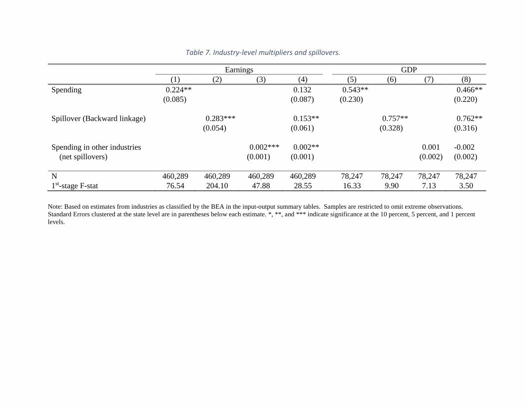
Table 7. Industry-level multipliers and spillovers.

Earnings GDP (1) (2) (3) (4) (5) (6) (7) (8)

Spending 0.224** 0.132 0.543** 0.466** (0.085) (0.087) (0.230) (0.220)

Spillover (Backward linkage) 0.283*** 0.153** 0.757** 0.762** (0.054) (0.061) (0.328) (0.316)

Spending in other industries 0.002*** 0.002** 0.001 -0.002 (net spillovers) (0.001) (0.001) (0.002) (0.002)

N 460,289 460,289 460,289 460,289 78,247 78,247 78,247 78,247 1st-stage F-stat 76.54 204.10 47.88 28.55 16.33 9.90 7.13 3.50

Note: Based on estimates from industries as classified by the BEA in the input-output summary tables. Samples are restricted to omit extreme observations. Standard Errors clustered at the state level are in parentheses below each estimate. *, **, and *** indicate significance at the 10 percent, 5 percent, and 1 percent levels.

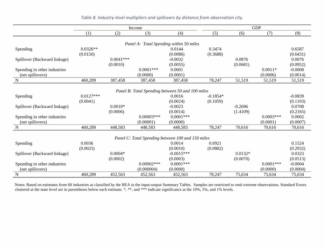
Table 8. Industry-level multipliers and spillovers by distance from observation city.

Income GDP (1) (2) (3) (4) (5) (6) (7) (8)

Panel A: Total Spending within 50 miles Spending 0.0326** 0.0144 0.3474 0.6587

(0.0150) (0.0086) (0.3688) (0.6431) Spillover (Backward linkage) 0.0041*** -0.0032 0.0876 0.0076

(0.0010) (0.0055) (0.0681) (0.0952) Spending in other industries 0.0001*** 0.0001 0.0011* -0.0008 (net spillovers) (0.0000) (0.0001) (0.0006) (0.0014) N 460,289 387,458 387,458 387,458 78,247 51,519 51,519 51,519

Panel B: Total Spending between 50 and 100 miles Spending 0.0127*** 0.0016 -0.1854* -0.0839

(0.0041) (0.0024) (0.1059) (0.1103) Spillover (Backward linkage) 0.0010* -0.0023 -0.2696 0.0708

(0.0006) (0.0014) (1.4109) (0.2165) Spending in other industries 0.00003*** 0.0001*** 0.0003*** 0.0002 (net spillovers) (0.00001) (0.0000) (0.0001) (0.0007) N 460,289 448,583 448,583 448,583 78,247 70,616 70,616 70,616

Panel C: Total Spending between 100 and 150 miles Spending 0.0036 0.0014 0.0921 0.1524

(0.0025) (0.0010) (0.0882) (0.2932) Spillover (Backward linkage) 0.0004* -0.0015*** 0.0132* 0.0323

(0.0002) (0.0003) (0.0070) (0.0513) Spending in other industries 0.00002*** 0.0001*** 0.0001*** -0.0004 (net spillovers) (0.000004) (0.0000) (0.0000) (0.0004) N 460,289 452,563 452,563 452,563 78,247 75,634 75,634 75,634 Notes: Based on estimates from 68 industries as classified by the BEA in the input-output Summary Tables. Samples are restricted to omit extreme observations. Standard Errors clustered at the state level are in parentheses below each estimate. *, **, and *** indicate significance at the 10%, 5%, and 1% levels.

Appendix Table 1. State-dependence of local multipliers.

Dependent variable: Labor earnings (1) (2) (3) (4) Spending 0.127** 0.109* 0.177** 0.245*** (0.055) (0.059) (0.083) (0.087) Spending × 1(UR≥25 percentile) 0.204* (0.121) 1(UR≥25 percentile) -0.017*** (0.002) Spending × 1(UR≥35 percentile) 0.246* (0.131) 1(UR≥35 percentile) -0.017*** (0.002) Spending × 1(UR≥50 percentile) 0.157 (0.119) 1(UR≥50 percentile) -0.017*** (0.002) Spending × 1(UR≥75 percentile) 0.091 (0.200) 1(UR≥75 percentile) -0.020*** (0.003) N 6093 6093 6093 6093 1st-stage F-stat 10.68 7.84 7.18 3.17

Notes: The table reports estimated effects of local defense spending on labor earnings depending on the state of the local economy. The state of the economy is measured with a set of dummy variables equal to one if the local unemployment rate is greater than or equal to a given cut-off. Column (1) uses the 25th percentile as the cut-off; that is, the unemployment rate for a given location has to be greater than or equal to the 75th percentile of unemployment rates observed for the location in our sample. Columns (2) through (4) use the 35th, 50th, and 75th percentiles respectively. 1(UR≥X percentile) denotes the dummy variable that is equal to one if the local unemployment rate is greater than or equal to the Xth percentile. The unit of observation is CBSA×year. Standard errors clustered at the state level are in parentheses below each estimate. *, **, and *** indicate significance at the 10%, 5%, and 1% levels.