management’s tone change, post earnings announcement drift ... · management’s tone change,...

Management’s Tone Change, Post Earnings Announcement Drift and Accruals

Ronen Feldman

Associate Professor of Information Systems Data & Text Mining Laboratory

Jerusalem School of Business Administration Hebrew University

Jerusalem, ISRAEL 91905 [email protected]

Suresh Govindaraj Associate Professor

Rutgers Business School – Newark and New Brunswick Department of Accounting, Business Ethics, and Information Systems

Ackerson Hall - Room 302B 180 University Avenue

Newark, New Jersey 07102-1897 Phone: 973-353-1017

e-mail: [email protected]

Joshua Livnat Professor of Accounting

Stern School of Business Administration New York University 10-76 K-MEC Hall

44 W. 4th St. New York City, NY 10012

(212) 998–0022 [email protected]

Benjamin Segal

Assistant Professor Accounting and Control Group

INSEAD Boulevard de Constance

Fontainebleau 77305, France Phone: +33 (0)1 60 72 92 45

[email protected]

First Draft: January 2008 Current draft: October 20, 2008

___________________________________ The authors gratefully acknowledge the Point-In-Time database provided by Charter Oak Investment Systems, Inc., and the S&P Filing Dates database provided by Compustat. The authors gratefully acknowledge comments made by seminar participants at Rutgers University and various colleagues at NYU.

mailto:[email protected]





Abstract

This study explores whether the Management Discussion and Analysis (MD&A)

section of Form 10-Q and 10-K has incremental information content beyond financial measures such as earnings surprises and accruals. It uses a well-established classification scheme of words into positive and negative categories to measure the tone change in a specific MD&A section relative to prior periodic SEC filings. Our results indicate that short window market reactions around the SEC filing are significantly associated with the tone of the MD&A section, even after controlling for accruals and earnings surprises. We also show that management’s tone change adds significantly to portfolio drift returns in the window of two days after the SEC filing date through one day after the subsequent quarter’s preliminary earnings announcement, beyond financial information conveyed by accruals and earnings surprises. We find that the incremental information of management’s tone change is higher when the firm’s information environment is weaker.


There is a substantial body of literature in financial economics and accounting

that examines the value relevance and information content of quantitative factors in the

pricing of stocks. While economic and statistical modeling has become more

sophisticated over the years, the somewhat disconcerting conclusion that seems to have

emerged is that these quantitative factors inadequately explain movement of stock prices.

Persuasive evidence of this is provided by Shiller (1981), Roll (1988), and Cutler et al.

(1989), and others in the finance literature, who demonstrate that stock prices do not

respond to change in quantitative measures of firm fundamentals as would be expected

from models incorporating only quantitative variables of firm performance. In the

accounting literature, Lev and Thiagarajan (1993), and Amir and Lev (1996), are two

examples of research that have shown the inadequacy of conventional quantitative

financial measures in pricing a firm’s stock. All in all, there is a growing realization that

in order to develop a “good” stock pricing model, one has to incorporate not only the

conventional quantitative measures of firm performance, but also include non-

conventional measures such as potential market share (Amir and Lev, 1996), and even

verbal, non-quantitative, difficult to quantify, kinds of measures.1

This is not totally surprising from a theoretical perspective. After all, stock prices

are set by investors who, by definition, compute prices as the discounted present value of

1 Though not directly connected to the research questions in our paper, we note that Boukus and Rosenberg (2006), and Hanley and Hoberg (2008), make a strong case for incorporating verbal and textual information in asset pricing models. While qualitative studies to date (including ours) make additional contribution to the explanatory power of stock return volatility, they do not completely fill the void left after one considers the financial quantitative measures.

future cash payoffs conditional on the current information set available to them. It seems

natural then to expect that the investor information set should include not only

quantifiable information, but also non-quantifiable, verbal information, such as news

articles. Indeed, Tetlock (2007) examines whether the general negative or pessimistic

flavor of a particular daily news column from the Wall Street Journal (WSJ) (titled

“Abreast of the Market”) covering the stock market activity on the previous day

influences prices of market indices of stocks. The depth of article pessimism is defined as

the proportion of negative words used in this column. After controlling for other

variables, he finds that the depth of pessimism in this column is correlated with a

significant downward (temporary) pressure on prices of the stock indices.2

Tetlock et al. (2008) further examines the ability of negative words used in WSJ

and the Dow Jones News Service (DJNS) columns about S&P 500 firms to predict future

earnings and stock returns on the day after the publication of these news articles. They

find that the proportion of negative words in these news stories (especially, negative

words about a firm’s fundamentals) do provide information about future earnings even

after controlling for other factors; the higher the proportion of negative words the larger

are the negative shocks to future earnings. In addition, they provide evidence that

potential profits could be made by trading on negative words from DJNS, a timely news

service (but not from the one day old information published in the WSJ).3

2 Following the initial impact on stock prices due to the media pessimism factor, the prices of indexes of smaller stocks reverse more slowly than those of large firms. In addition, he also provides evidence to show that pessimism is not a proxy for risk. As an additional feature, he also finds that unusually high or low pessimism among investors leads to temporarily high trading volume. 3 The authors acknowledge that these profits could be wiped out by transactions costs from high frequency trading.

2

The two Tetlock papers remain among the first of their kind to assess the

predictive content of non-quantitative verbal information, and are the main motivators of

our work.4 By focusing on news stories in media, their work is more concerned with

pessimism expressed by outsiders (media-persons), except for press releases issued by the

firms. While these papers make a strong case for the predictive value of pessimism

expressed by outsiders on stock prices and future earnings, they may not completely

capture the views of mangers (or insiders), who are required to express their views in

Securities and Exchange (SEC) filings. It can be argued that managers are better

informed than outsiders, and assuming that they truthfully report their views (under SEC

scrutiny and penalty of litigation), their statements may have higher predictive ability

than outsiders’ reports.5

Our study investigates the information content of the “tone” change conveyed

through Management Discussion and Analysis (MD&A) disclosures for a large sample of

firms. By “tone” change, we mean the pessimism or optimism of the information

embedded in non-quantifiable verbal disclosures by managers in the MD&A section of

firms’ periodic SEC filings as compared to prior periodic filings of the same firm. We

focus on the effects of management’s tone change on immediate and delayed stock

returns beyond what is captured by preliminary earnings surprises and accruals, the two

4 We note that Abrahamson and Amir (1996) perform a content analysis of over 1,300 President’s Letters to shareholders for firms trading in the NYSE and written between 1986 and 1988. They show that while the relative “negative” content of the letter (measured by a proprietary computer program) reflects past performance of a firm and is priced by the market, it can also (weakly) predict future firm performance. 5 Kothari and Short (2003) is probably the first paper to recognize this and examine the information content of MD&A disclosures in addition to the information content of analysts forecasts and media reports using a methodology similar to Tetlock (2007) and Tetlock et al. (2008). However, they focus on the effects of the MD&A’s sentiment on the firm’s cost of capital and risk (stock price volatility), not on their ability to predict future stock prices and earnings.

3

accounting variables best known to be informative about the future stock performance of

the firm.6

We find that the change in tone of the MD&A section of the SEC filings from

prior periodic filings, in fact, contains information orthogonal to accruals and earnings

surprises. We show by regression analysis and by explicit construction of buy and hold

portfolio strategies, that the optimism, pessimism, and especially the differential

optimistic tone change measure (the change in optimism net of pessimism), yield excess

average stock returns over the short window following the filing of the MD&As, but also

that returns continue to drift for longer periods that extend until after the subsequent

quarter’s preliminary earnings announcement. As can be expected, the change in MD&A

tone is incrementally more informative when the information environment surrounding

the firm (as measured by size and analyst following) is weaker. The tone change is also a

weaker signal for value firms, which are typically more mature and easier to understand.

We also find the tone change signal to have stronger implications for firms with positive

earnings surprises, probably because these are cases where investors may need additional

information beyond the quantitative disclosure. The implication is that the non-

quantitative tone change expressed in MD&As can be potentially exploited to earn

significant excess returns over and above those associated with well known trading

strategies based on accruals and earnings surprises alone.

Our results contribute in general to research on the information content and value

relevance of SEC filings and mandated disclosures. Specifically, our paper contributes to

the value relevance of disclosures in the MD&A statements. To the best of our

6 In an earlier version, we had also controlled for operating cash flows (OCF) with similar results to those obtained here.

4

knowledge, we are the first to measure and show that the tone change expressed by

management through non-quantifiable words in MD&A is associated with immediate

market reactions and can also predict future stock prices beyond well-known measures of

company performance. Our findings should be of interest to academics who are interested

in such issues as market efficiency and how well public (especially non-quantitative)

information is captured in security prices, and to those academics who are concerned with

the effects of the information environment on the associations between public

information and security returns. The results of our study are also relevant to policy-

makers because it shows the incremental valuation relevance of required non-quantitative

information. Since the tone change in SEC filings (which are filed regularly) can be used

to improve portfolio performance beyond quantitative variables, our results should

interest practitioners as well.7

The rest of the paper is organized as follows: The next section reviews the

relevant literature and motivates our research hypotheses. Section 3 describes the sample,

defines and describes the variables used in our paper. Section 4 presents our results and

Section 5 concludes our paper.

2. Prior Research and Research Questions 2.1 Prior Research

Broadly speaking, there are two kinds of research relating to the valuation of

corporate disclosures in the accounting literature, namely, the voluminous body of work

that has examined the value relevance (or information content) of financial disclosures,8

7 The set-up costs required for analyzing the tone change of qualitative disclosure may favor professional investors. 8 We refer the interested reader to the book by Beaver (1997) for a discussion and analysis of the value relevance of financial disclosures.

5

and the relatively smaller set of research papers that have studied the valuation of non-

financial disclosures. Within the set of studies of value relevance of non-financial data

there are two major sub-sets; namely, those that focus on quantifiable data, and those that

examine non-quantifiable verbal expositions that elaborate and explain quantitative

disclosures. Our research examines the information content of narratives from MD&A

and so is related to the latter stream of research, the value relevance of non-financial,

non-quantifiable disclosures. However, in examining the incremental value relevance of

MD&A disclosures, we also control for the value relevance of financial variables that

have been extensively documented by prior studies.

We cite two papers that examine the incremental information content of

quantifiable non-financial information.9 Using a large sample of firms from 1974-1988,

Lev and Thiagarajan (1993) show that certain non-audited but quantifiable information,

such as order backlogs and the strength of their labor force, provide information for

company valuation over and beyond the traditional financial accounting information.

Amir and Lev (1996) further build on this theme by studying the value relevance of

financial and non-financial data for a sample of wireless communication firms and find

that financial data alone show very little value relevance, but if combined with

quantifiable non-financial data (specifically, proxies for potential customers) the value

relevance of these financial variables are considerably enhanced.

Some of the early research relating to MD&A is mostly descriptive in its content.

Bagby et al. (1988) provide a historical review of MD&A and the social usefulness of

non-quantitative disclosures within a broader framework of federally mandated

disclosures using a critical examination of legal cases relating to mandated disclosures. 9 These papers provide citations for the interested reader.

6

Dieter and Sandefur (1989) outline the MD&A requirements mandated by the SEC and

suggest guidelines on drafting a MD&A that would satisfy these regulations in form and

substance. Sanders and Das (2000) discuss the electronic filing rules as instituted by the

Securities and Exchange Commission (SEC) and the Electronic Data Gathering,

Analysis, and Retrieval (EDGAR) system in detail.

Shroeder and Gibson (1990) is among the earliest papers to try and quantify the

readability quotient of the exposition in the MD&A and also the President’s letter.

Borrowing techniques from the Psychology literature, they construct the so-called Flesch

Index scores (a presumably reliable subjective measure of reading ease) using a standard

formula based on the word length and sentence length, and by also examining the general

flavor of the language used (active versus passive voice in sentence constructions), they

conclude that MD&A statements in general are less than readable.

One of the earliest papers in the accounting literature that use linguistic

techniques to analyze narrative disclosures is Frazier et al. (1984). Using a computer

program called WORDS to identify the most important words (or factors) that could be

reasonably interpreted as positive or negative narrative themes for a sample of 74 annual

reports of firms in 1978 they show that there are no significant differences in managerial

narratives across the ownership structure of these firms. They also provide evidence to

support their hypothesis that the positive and negative factors (and the associated themes)

can predict the cumulative abnormal annual returns for the next year (1979).10

Motivated by SEC requirements that firms provide easy to read and plain

disclosures, Li (September, 2006) extends this line of enquiry by examining whether the

readability and the writing style of annual corporate reports of a large sample of firms 10 The paper also discusses other applications of WORDS in finance and accounting.

7

during the years 1993 to 2003 can predict future firm earnings and returns. Using

measures from linguistics for readability and writing styles, Li concludes that firms with

poor performance put out hard to read reports, profitable firms with more complicated

reports have a lower persistence of earnings, but these measures do not correlate with

future stock returns.

Pava and Epstein (1993) study the MD&A disclosures of 25 randomly selected

firms during 1989 and find that while the disclosures provided adequate details of

historical events, they did a better job of predicting firm specific, industry specific, and

economy specific good news than predicting bad news for 1990. They conclude that

managers may be withholding disclosures related to bad news. While these studies are

related to our work, their samples are small and limited to specific early years prior to

revised SEC’s guidelines on MD&A and the availability of SEC filings on EDGAR.

In 1989, the SEC issued guidelines to clarify what was expected in the MD&A

disclosures in an attempt to make the MD&A more informative. Hooks and Moon (1993)

attempt to measure the differences between actual and expected frequency of MD&A

disclosures across a spectrum of disclosures that they classify as mandated to those that

are classified as voluntary, and show that these differences have decreased for certain

items after the SEC MD&A guideline release in 1989, indicating firms provide more

disclosure in their MD&A post 1989.

Bryan (1997) examines if the specific accounting related narratives from MD&A

have incremental information content beyond quantitative financial statement information

regarding future financial variables such as the directions of changes in future sales,

future earnings per share, future operating cash flows, and future capital expenditures.

8

Using a sample of MD&A disclosures by 250 firms in 1990 (a year after clearer

guidelines were issued by the SEC), he finds that there is a strong association between

MD&A disclosures and the direction of changes in the aforementioned future financial

variables three years into the future. In addition, he demonstrates that MD&A

disclosures, especially the disclosure relating to capital expenditures, are significantly

associated with financial analyst forecasts and stock returns around the release date of

MD&As. Bryan’s paper differs from our work in that we are interested in the predictive

ability of the overall tone change of the MD&A rather than the contents of individual

MD&A disclosures. He does not examine if abnormal stock returns can be earned or

study the issue of post announcement drift in stock prices. Further, the content analysis

by Bryan is subjective as opposed to the more objective tone change index used here and

by Tetlock (2007) and Tetlock et al. (2008). Finally, our sample size is much larger and is

drawn from years when the legal and disclosure environments are substantially different.

There are few papers that examine the relationship between MD&A disclosures

and analyst forecasts. One such paper is by Barron and Kile (1999). Using a large sample

of firms drawn from 1987-1989 MD&A disclosures of 26 different industries, and after

controlling for quantitative financial factors, they show a strong association between the

accuracy of analysts’ forecasts and the quality of MD&A disclosures (as measured by

scores assigned by personnel at the SEC), especially disclosures relating to capital

expenditures. Clarkson et al. (1997) document that MD&A disclosures are found to be

useful to sell-side analysts who are members of the Toronto Society of Financial Analysts

(TSFA) based on 33 responses to questionnaires. In addition, using a sample of 55 firms

on the Toronto Stock Exchange (TSE) between 1991 and 1992, they show that the

9

levels and the changes in the quality of various sub-sections of the MD&A disclosures

(where the quality of disclosures is a score provided by the members of TSFA) are

generally determined by expected firm performance, financing activities (mainly

increased equity financing), firm size, independent press reports, and major firm related

events.

Cole and Jones (2004) use MD&A disclosures from a sample of 150 firms for the

period 1996-1999 from the retail industry to show that certain types of quantifiable

disclosures, (namely sales growth, store openings and closings and capital expenditures),

can predict future profitability, and are associated with contemporaneous stock returns.

Sun (2007) examines the MD&A disclosures explaining inventory increases between

1998 and 2002 for 568 manufacturing firms and shows that favorable explanations are

associated with future profitability and sales growth, and firms in growth industries and

competitive industries tend to disclose more.

Kothari and Short (2003) is perhaps the first accounting work to have used the

General Inquirer program (which we use in this study) to assess the effects of the tone (as

opposed to tone change used in our paper) expressed in MD&A disclosures on the firm’s

cost of capital.11 They extend the work of Botosan (1997) by studying the effect of the

positive and negative sentiments expressed in MD&A, analyst reports, and the financial

press between 1996 and 2001 on the cost of capital and risk (stock price volatility) for a

sample of 887 firms from 4 industries (Technology, Telecommunications,

Pharmaceutical, and Financial). They find that aggregated (across all three sources)

11 Since managers usually use prior MD&As as a blueprint for producing a new and incremental MD&A, there could be considerable similarities in MD&As that are close in years. This suggests that our tone change measure may be a better measure of information content than the tone level measure used by Kothari and Short (2003).

10

positive (favorable) disclosures decreased the cost of capital and the stock return

volatility of the firm, while negative (unfavorable) disclosures had the opposite effects.

However, when disclosures are analyzed by sources, they find that positive sentiments

expressed in corporate MD&As do not have an effect on the cost of capital, while

negative sentiments significantly increase it. They attribute this to skepticism on the part

of investors regarding positive disclosures (that is they are viewed more as self serving),

but find negative sentiments credible because management would not normally reveal

bad news. Disclosures relating to analysts’ sentiments seem to have no effect on the cost

of capital, and this is attributed to the lack of credibility. They attribute this to the fact

that analysts are seen to be reporting their sentiments after the market has already

absorbed them. Finally, they find that positive media (press etc.) stories and disclosures

seem to decrease the cost of capital and negative disclosures increase it.12 Related to this

line of enquiry, is the study by Li (April, 2006) that examines whether the risk sentiments

and change in risk sentiments expressed in annual reports are associated with future firm

performance and future stock returns. Using a large sample of annual reports from 1994

to 2005, Li constructs an intuitive quantitative measure of levels and changes in risk

sentiments extracted from the text of these reports, and finds large increases in risk

sentiments to be associated with lower future earnings and significant lower stock

returns.

We note that our paper differs from Kothari and Short (2003) in that we are not

interested in analyzing the effects of soft disclosures on the firm’s cost of capital or the

variability of stock returns. We are also different from Li (2006) who is interested in the

12 This supports the findings of Tetlock (2007) who shows similar results for a market index (Dow Jones Index), that is when the media reports are pessimistic, the stock index price drops and market volatility increases.

11

incremental effects of the subjective measures of references to risk changes in annual

reports (including the MD&As) on future stock prices and earnings. We are not

concerned with any measure of risk, but rather with the incremental effects of general

tone changes in MD&As on immediate and future stock returns.

As mentioned before, the two papers that are closest in spirit to ours are by

Tetlock (2007) and Tetlcok et al. (2008). They do not focus on pessimism and predictive

content of MD&As but on news columns and news releases. Tetlock (2007) uses a

computer program known as the General Inquirer to assess the negative quotient of the

Wall Street Journal daily column called “Abreast of the Market” from 1984 to 1999, and

finds results consistent with pessimistic articles putting temporary downward pressures

on market prices (Dow Jones stock index) and increasing trading volume in the New

York Stock Exchange (NYSE). The increased volume of trade is consistent with

microstructure theory that predicts high absolute values of pessimism should lead to a

group of liquidity traders trading more, and refutes the suggestion that the pessimism

factor is a proxy for transaction costs (Tetlock, 2007).13 It is important to note that

Tetlock (2007) finds higher pessimism leads to higher volatility (risk) for the Dow Jones

portfolio of stocks. This goes against the intuition that higher pessimism should lead to

lower returns, or equivalently, lower risk, suggesting that the pessimism factor captured

by negative words may be distinct from risk. This is further corroborated by the fact that

the effects of pessimism seem to be temporary and future stock returns reverse.14

Continuing this line of research, Tetlock et al. (2008) examine the ability of media

13 If the pessimism factor were a proxy for transactions costs, then higher levels of pessimism should lead to lower volumes of trading on the following periods (see Tetlock, 2007) 14 This reversal seems to be slower for small firms’ stocks relative to stocks of big firms when the tests are run on stocks other than those in the Dow Jones Index.

12

pessimism measured by the proportion of negative words in the real time stories news

from DJNS and daily news stories in the WSJ between 1984 and 2004 relating to S&P

500 firms to predict future earnings and returns. They show that the change in the

proportion of negative words (especially those relating to firm fundamentals) in these

news releases do convey information about firm future earnings. They also find that the

proportion of negative words in the timely news releases from DJNS leads to lower stock

returns the following trading day and this trend persists over the next 10 days. These

results remain robust even after controlling for other sources like analysts’ forecasts, past

stock returns, and historical accounting data. The authors show that a simple trading

strategy of constructing portfolios that short stocks of firms with negative words in the

DJNS news stories the previous day and long on the stocks with relatively few negatively

worded stories produces significant abnormal returns (excluding transactions costs).

Demers and Vega (2007) extend the analysis in the Tetlock (2007) and Tetlock et

al. (2008) by examining the incremental information content of sentiments expressed in

“soft” or “verbal” text in voluntary, non-mandated management’s quarterly press

releases. Using a different linguistic program, the Diction 5.0, to extract the sentiments

expressed in almost 15,000 corporate earnings announcements over the period from 1998

to 2006, they show that “unexpected” sentiment does have incremental information

content in partially explaining the well known post announcement earnings drift in

market prices. Further, they provide evidence suggesting that the lack of clarity in press

releases seems to be associated with abnormal trading and increased trading volumes.

Engelberg (2008) is another extension of the Tetlock (2007) and Tetlock et al. (2008)

papers. Using a large sample of earnings announcements in the Dow Jones Index

13

obtained from the Factiva database for the period 1999 to 2005, he shows that “hard to

understand” textual qualitative information is value relevant, and contributes uniquely to

the well known post earnings announcement drift phenomenon. He further shows that the

harder the textual information is to understand and process, the more slowly it diffuses

into prices. Davis, Piger, and Sidor (2008) is another paper that examines the tone of

23,400 quarterly earnings press releases published on the PR Newswire between 1998

and 2003 using the linguistic program Diction.15 They find that there is a significant

positive (negative) association between increased optimism (pessimism) and future

measures of firm performance (measured by the Return on Assets), and increased

optimism (pessimism) is positively (negatively) associated with market returns around

the announcement dates. Using a sample of firms from the telecommunications and

computer services industries, and related equipment manufacturers for the period 1998 to

2002, Henry (2007) also finds that the tone and style of press releases incrementally

influences short window stock prices.16

It should be noted that these studies examine the preliminary earnings

announcements by firms, rather than the MD&A sections of periodic reports as we do.

The preliminary earnings announcements were typically not filed with the SEC prior to

2003, and, therefore, not routinely scrutinized by the SEC as periodic reports were.

Further, preliminary earnings announcements are voluntary, and some firms do not issue

them at all, or issue them sporadically. In contrast, periodic reports must be filed with the

15 Some of the other papers that use Diction to extract investor sentiment are Bligh and Hess (2007), Ober et al. (1999), Yuthas, Rogers, and Dillard (2002). 16 Henry (2007) uses a metric for tone that is similar to the one used in our paper. Others, notably, Das et al. (2004), and Das and Chen (2004), examine the association between stock price movements and online discussions and news activities using their own tone (or sentiment) index based on 5 distinct natural language processing algorithms that classify such discussions as bullish, bearish, or neutral .

14

SEC by all firms. Finally, the MD&A sections are intended to disclose qualitative

information by management, which the preliminary earnings announcements frequently

do not have. Furthermore, even in cases where preliminary earnings announcements

contain qualitative information, they frequently do not include information on the same

items in a consistent manner, because unlike MD&A section, preliminary earnings items

are voluntary and additional information about them is not required by SEC rules.

In related research, Abrahamson and Amir (1996) perform content analysis of

over 1,300 President’s Letters to shareholders for NYSE firms written between 1986 and

1988. They show that relative negative content of the letter (measured by a proprietary

computer program) is strongly negatively associated with past and future performance as

measured by accounting variables, strongly negatively associated with past and

contemporaneous (yearly) returns, and weakly negatively associated with future returns.

2.2 Research Questions

Investors in stocks may be able to exploit disclosures of accruals and earnings

surprises (usually constructed as a standardized measure of an abnormal earnings metric

or SUE) immediately (short window) following these disclosures, and over the longer

term as well. Of the two, the influence of earnings surprises on stock prices is perhaps the

oldest and best documented phenomenon. It has been repeatedly shown that positive

(negative) earnings surprises exert immediate upward (downward) pressure on prices and

surprisingly, this trend continues to persist for a long time after the initial disclosure (the

post-announcement drift anomaly). Investors can exploit this anomaly by holding

differential positions of stocks with extreme positive and negative SUEs (see Livnat and

15

Mendenhall, 2006, for a recent comparison of SUE based on time series and analyst

forecasts).

In addition to earnings surprises, the accounting and finance literature has also

documented the information relevance of accruals. Sloan (1996) shows that firms with

extremely low annual accruals outperform firms with extremely high accruals. His study

was corroborated by many subsequent studies with annual accruals and by Livnat and

Santicchia (2005) with quarterly accruals. Collins and Hribar (2000), and more recently

Battalio et al. (2007), show that earnings surprises and accruals are two distinct

anomalies and using each yields incremental abnormal returns beyond the other.

Our research examines if the tone change expressed in MD&A disclosures is

associated with contemporaneous and future abnormal returns (short window following

the MD&A disclosure and the post announcement long term drift) over and above what is

associated with preliminary earnings reports (SUE) and accruals. In the spirit of Tetlock

(2007) and Tetlock et al. (2008), we define a pessimistic tone change (signal) as the

change in the proportion of negative words among all words in the MD&A relative to the

average pessimistic signal in all periodic SEC filings made in the prior 400 days (scaled

by the standard deviation of the signal in the same period). The larger this proportion, the

more pessimistic is the tone change. We also define a similar measure for optimistic tone

change and further define a differential optimistic tone change measure by taking the

change in the difference of the positive and negative words divided by the sum of

positive and negative words in the MD&A relative to the average of this measure in all

periodic SEC filings made in the prior 400 days (scaled by the standard deviation of the

signal in the same period).

16

Our control variables are SUE and accruals which we measure as in the prior

literature. When there are no analyst forecasts for the quarter, SUE is calculated from the

Compustat quarterly database as preliminary income (Quarterly item 8) for quarter t

minus as-first-reported income for quarter t-4, scaled by the market value of equity at the

end of the quarter. When there is at least one analyst forecast for quarter t on IBES, the

SUE is calculated as the actual I/B/E/S unadjusted EPS minus the mean analyst forecast

during the 90-day period before the disclosure of earnings, scaled by the price per share

at the end of the quarter. Accruals/Average Assets equals income before extraordinary

items and discontinued operations minus cash from operations (OCF), scaled by average

total assets during the quarter.

We also investigate whether the information environment affects the associations

between the tone change signals and security returns. It is expected that the tone change

signal would be more effective for firms that are less heavily followed by analysts, that

are smaller, and that are more growth-oriented because their information environments

are weaker, leading investors to utilize other information, even the more stale information

provided by management in the SEC filings after the preliminary earnings releases (and

potentially the following conference calls with analysts).

We show that there are significant incremental abnormal returns around the filing

date and for the long term drift by constructing buy and hold type portfolio strategies that

incorporate the tone change factor in addition to the SUE and accruals, as well as by

running quarterly regressions as in Fama-Macbeth (1973)17.

17 Short window abnormal returns surrounding MD&A disclosures are defined as buy and hold return on a stock minus the average return on a matched size-B/M portfolio over the days [-1,+1], where day 0 is the SEC filing date. The excess drift return for the longer term is the buy and hold return on a stock minus the

17

3. Data and Sample Selection

3.1 The Preliminary and Un-restated Compustat Quarterly Data

Data entry into the Compustat databases has been performed in a fairly structured

manner over the years. When a firm releases its preliminary earnings announcement,

Compustat takes as many line items as possible from the preliminary announcement and

enters them into the quarterly database within 2-3 days. The preliminary data in the

database are denoted by an update code of 2, until the firm files its Form 10-Q (10-K)

with the SEC or releases it to the public, at which point Compustat updates all available

information and uses an update code of 3. Unlike the Compustat Annual database, which

is maintained as originally reported by the firm (except for restated items), the Compustat

Quarterly database is further updated when a firm restates its previously reported

quarterly results. For example, if a firm engages in mergers, acquisitions, or divestitures

at a particular quarter and restates previously reported quarterly data to reflect these

events, Compustat inserts the restated data into the database instead of the previously

reported numbers. Similarly, when the annual audit is performed and the firm is required

to restate its previously reported quarterly results by its auditor as part of the disclosure

contained in Form 10-K, Compustat updates the quarterly database to reflect these

restated data.

Charter Oak Investment Systems, Inc. (Charter Oak) has collected the weekly

original CD-Rom that Compustat sent to its PC clients, which always contained updated

value weighted average return on a matched size-B/M portfolio from two days after the SEC filing date through one day after the subsequent quarter’s preliminary earnings announcement.

18

data as of that week. From these weekly updates, Charter Oak has constructed a database

that contains three numbers for each firm for each Compustat line item in each quarter.

The first number is the preliminary earnings announcement that Compustat inserted into

the database when it bore the update code of 2. The second number is the “As First

Reported” (AFR) figure when Compustat first changed the update code to 3 for that firm-

quarter. The third number is the number that exists in the current version of Compustat,

which is what most investors use. The Charter Oak database allows us to use the first-

reported information in the SEC filing, so that quarterly earnings, cash flows and accruals

correspond to those reported originally by the firms, which were also available to market

participants at the time of the SEC filing. Using the restated Compustat Quarterly

database may induce a hindsight bias into back-tests, since we may have used restated

earnings, cash flows or accruals that were not known to market participants on the SEC

filing dates.

3.2 Sample Selection

To reduce the potential bias that may occur by using a sample of quarterly

information that became available through SEC filings before the SEC’s EDGAR

database and afterwards, this study concentrates on SEC filings that are available through

the EDGAR database from the fourth quarter of 1993 through the second quarter of 2007.

Conceptually, information in SEC filings on the SEC EDGAR database is likely available

to users at a low cost immediately after the filing date indicated in the EDGAR

database.18, 19 Prior to EDGAR, information about SEC filings was available from the

companies directly or from the SEC library with a lag (see, e.g., Easton and Zmijewski,

18 The low costs should especially apply to professional investors. 19 The interested reader can refer to Sanders and Das (2000) for guidelines regarding the filing formats for the SEC, the definition of the filing sate, other important details regarding filings and the EDGAR database.

19

1993). The problem with the SEC EDGAR database is that it identifies firms according to

CIK codes, which are not well-mapped into other databases used in practice and academe

such as Compustat or CRSP.

The Standard & Poors’s (S&P) Filing Dates database seeks to fill this void.20 It

contains a match between all companies on the Compustat database (identified by

GVKEY) with the CIK identifiers on the SEC EDGAR database.21 The S&P Filing Dates

database matches all Compustat firms (by GVKEY) to CIK codes on the SEC EDGAR

database as they were known on the Compustat database at the time through the Charter

Oak database. Thus, it is useful in constructing a universe of firms that professional

investors could have actually been using at the time without survivorship bias. For each

10-K and 10-Q filing on EDGAR, the database includes not only the SEC filing date but

also the balance sheet date for the quarter/year, so an accurate match with Compustat

information can be made.22

For each firm-quarter in the S&P Filing Dates database we obtain the SEC filing

dates for the period Q4/1993-Q2/2007. We include in our sample only those SEC filings

made within 55 (100) days for 10-Q (10-K) forms to ensure exclusion of delayed filings.

We further limit the sample to observations with SEC filing dates for initial 10-Q/10-K

filings in the S&P Filing Dates database which also have a matching GVKEY on

Compustat and a matching PERMNO on CRSP, so we can retrieve financial statements

data from Compustat and stock return data from CRSP. We further reduce the sample to

firms that are listed on NYSE, AMEX or NASDAQ and have a market value of equity

20 The database is available through WRDS or directly from S&P. 21 The database includes all GVKEY’s where the market value of the firm’s equity at quarter-end exceeded $1 million. 22 Because companies may file their 10-Q forms late, the filing date itself cannot be a reliable indication for the specific quarter it relates to.

20

and average total assets at quarter end, as well as total assets during the quarter in excess

of $10 million, and quarter- end price per share in excess of $5. We further delete

observations if the originally reported income before extraordinary items and

discontinued operations (Compustat Quarterly item No. 8) is missing; or the originally

reported quarterly net operating cash flow (Compustat Quarterly item No. 108) is

missing; if market value at the end of the prior quarter is unavailable; or if total assets

(Compustat Quarterly item No. 44) at the end of the prior quarter or at the end of the

current quarter are missing. Table 1 provides details on our sample selection.

3.3 Variable Definitions

To reduce the survival bias, we use holding periods of 90 days after the SEC

filing date if the subsequent quarterly earnings announcement date is missing. If a

security is de-listed from an exchange before the end of the holding period, we use the

delisting return from CRSP if available, and -100% if the stock is forced to de-list by the

exchange or if the delisting is due to financial difficulties. After delisting, we assume the

proceeds are invested in the benchmark size and B/M portfolio. This is the procedure

used by Kraft, et al. (2004). We first calculate the buy and hold return on the security

during the holding period; then subtract the buy and hold return on a similar size and B/M

benchmark portfolio for the same holding period. The benchmark returns are from

Professor Kenneth French’s data library, based on classification of the population into six

(two size and three B/M) portfolios.23, 24

23 http://mba.tuck.dartmouth.edu/pages/faculty/ken.french/data_library.html . 24 To make sure that our results are not driven by observations with extreme returns as argued by Kraft et al (2004), we repeated the analysis but deleted all extreme 0.5% observations with buy and hold excess returns in any of the two return periods used. The results are qualitatively similar to those reported here.

21

http://mba.tuck.dartmouth.edu/pages/faculty/ken.french/data_library.html

Consistent with the accruals literature, we estimate accruals as earnings minus net

operating cash flows, and scale by average total assets during the quarter. Accruals are

based on the first-reported data in the Charter Oak database, and are not subject to

Compustat’s subsequent restatement of data. We estimate the preliminary earnings

surprise as IBES (unadjusted for splits) actual EPS minus mean forecasted (unadjusted

for splits) EPS by all analysts with quarterly forecasts in the 90-day period prior to the

preliminary earnings announcement, scaled by price per share at quarter end. If there are

no analyst forecasts of earnings on IBES, we use preliminary net income (Compustat

quarterly item No. 8) minus net income as reported for the same quarter in the prior year,

scaled by market value of equity at the end of the previous quarter.

To eliminate the undue influence of outliers and to estimate the returns on hedge

portfolios constructed according to various signals, we independently sort all firms into

quintiles of various signals each quarter. We then use the scaled quintile rank as the

independent variable in regression equations, where the scaling is performed by dividing

the ranked quintile (0-4) by 4 and subtracting 0.5. Thus, the intercept in regressions of

returns on the signal should be equal to the mean excess buy and hold returns (BHR) for

the period, and the slope coefficient on the signal represents the return on the hedge

portfolio that is long the highest signal quintile and is short the bottom signal quintile.

To obtain signals about the “tone” change of the MD&A section in the 10-Q or

10-K, we extract the MD&A section from the relevant SEC EDGAR filings and count the

number of words in the section. The process begins by identifying all initial (rather than

amended) SEC filings that contain the prefix 10-Q, 10Q, 10-K, or 10K, and which were

filed in a timely manner (within 55 (100) days from the 10-Q (10-K) report date. These

22

filings were first matched to Compustat and CRSP to ensure data availability for our

quantitative variables. We have used a PERL program to retrieve the MD&A section

from each relevant SEC filing. To identify the MD&A section within a 10-Q or a 10-K

filing, we use the surface patterns (item number, titles, surrounding language, and new

item number to indicate end of section) in dozens of examples which were used to

develop general retrieval rules that were tested on another sample, where it obtained an

accuracy rate of over 99% in identifying the MD&A section. We first convert certain

HTML codes into characters, such as “&amp” into “&”, and eliminate all other

embedded HTML codes. We proceed to process only the remaining embedded text in

counting words. We eliminate cases where the total number of words in an MD&A

section is less than 30. We count the number of “positive” and “negative” words as

classified by the Harvard’s General Inquirer, after properly handling prefixes and

suffixes.25 We define three main variables as our signals, the number of “positive”

(“negative”) words, POS (NEG), divided by the number of total words, and (POS-

NEG)/(POS+NEG). To identify changes in the “tone” of MD&A from past filings and to

scale signals properly for their variability, we subtract from each signal the mean signal

in periodic SEC filings made within the preceding 400 calendar days, and divide by the

standard deviation of the signal in the periodic SEC filings made within the preceding

400 calendar days. Because the MD&A sections of periodic filings are expected to vary

little from one period to another, we do not use the proportion of the number of negative

(positive) words, but its change from the past. When management is aware of changes

that occurred during the current period from prior periods (such as declining sales, new

products, additional expenses, new liquidity concerns), it is likely to discuss those 25 See description and categories in http://www.wjh.harvard.edu/~inquirer/homecat.htm.

23

changes in the current MD&A, leading to tone changes from previous periodic filings.

Note that the benchmark we use to standardize the proportion of positive (negative)

words is the average of the signal in the MD&A sections of prior periodic (10-Q and 10-

K) filings, because other filings such as immediate reports (Form 8-K), registration

statements, proxies, etc. are likely to include other words and their average signal is

likely to be affected by the reason for the filing. Note that we use the standard error of the

signal in the periodic filings made in the prior 400 days, ensuring that we must have at

least three such periodic filings to estimate the tone change used in the current study.26

We expect high scores on the POS and (POS-NEG) signals to have higher immediate and

subsequent returns than those with low scores. Conversely, we expect immediate and

subsequent returns on high NEG scores to be lower than those on low NEG scores.

Consistent with prior results, we expect firms with high scores on earnings surprises to

have greater immediate and subsequent returns than those with low scores. The converse

should hold for accruals.

Table 1 shows that, our initial sample had 382,435 SEC filings which start with

10-K, 10K, 10-Q or 10Q on the June 2008 version of the S&P SEC Filing Dates Database

that are not amended filings and are not more than 100 (55) days after the fiscal year

(quarter) end. Merging with the Compustat Point-In-Time File, requiring a valid CUSIP,

market value of equity at quarter-end in excess of $10 million, and average total assets

during the quarter in excess of $10 million, price per share at quarter-end in excess of

$5.00, and an available earnings surprise reduced the sample size to 218,524

observations. Including only observations with filing date short-window excess returns

26 We first estimate the signal for each periodic filing in a specific quarter, and then use the prior periodic filings to estimate the tone change. Thus, all means and standard errors are based on initial 10-Q and 10K forms, and not their subsequent amendments.

24

around the SEC filing (i.e., days [-1, +1] where day 0 is the SEC filing date), and drift

returns from two days after the SEC filing through one day after the preliminary earnings

announcement for the subsequent quarter, and eliminating observations before Q4/1993

and after Q2/2007 due to scarce number of observations in these quarters, yields a sample

of 201,285 firm-quarters. For 192,592 observations, the MD&A section has more than 30

words and the positive, negative, and differential tone signal can be computed. However,

requiring the tone change variable further reduced the final sample size to 153,820

observations (firm-quarters), with 689 in Q4/1994 (minimum per quarter in our sample)

climbing to a high of 4,008 in Q1/1998 (the maximum for a quarter). Thus, there is

sufficient number of observations for each of the quarters in our sample period to

construct meaningful portfolios.

(Insert Table 1 about here)

Table 2 provides summary statistics about our sample. As can be seen, our sample

consists of firms with a wide distribution of sizes. The sample median market value is

$454 million and the mean is $3.239 billion. The median price per share is $20.97 with a

mean of $42.95; recall that there is a minimum price per share of $5.00 for sample

inclusion. Thus, we have a wide distribution of firm size and price per share. About 2/3

of the observations (103,569) have quarterly forecasts on IBES, with a median coverage

by two analysts. Consistent with prior studies the mean and median accruals are negative,

largely due to the effects of depreciation. The mean and median SUEs are roughly zero

indicating that our earnings forecast models are reasonably good for the median firm. It is

interesting to note that the number of positive words is usually greater than the number of

negative words in MD&A disclosures, indicating a possible optimistic tone in MD&A

25

disclosures on average. This also requires us to adjust for “expected” number of

positive/negative words by subtracting the mean signal in the prior 400 days. The positive

and negative signals indicate a slight skewness, with the means slightly larger than the

medians.


4. Results

Table 3 shows the mean excess returns for three subgroups of our sample firms

formed using different signals, where mean excess returns is defined as the BHR on a

stock minus the average returns on a matched size-Book to Market (B/M) portfolio over

the days [-1. +1], with day 0 identified as the SEC filing date. Firms are classified into

three groups using the bottom 20%, middle 60%, and top 20%. Consistent with the prior

literature about short window reactions around the preliminary earnings announcement,

firms in the bottom (top) SUE quintile have a mean excess return of -0.6% (+0.3%) in the

three-day window centered on the SEC filing, with an even stronger spread for earnings

surprises calculated from analyst forecasts. The top and bottom quintiles have statistically

different mean excess returns as indicated by the rightmost column. In contrast, we do not

observe any such differences for the accruals signal, although the accrual anomaly is not

for the short-window around the SEC filings but for subsequent returns.


The interesting observation in this table pertains to the tone change signals in the

MD&A sections. Both positive and negative sentiments are associated with significant

short window mean excess returns in the expected direction. The bottom (top) negative

tone change quintile has mean excess returns for the short window around the SEC filing

26

of 0.0% (-0.2%), with the means statistically different across the two extreme quintiles.

The converse is evident for the positive and (positive-negative) signals, where the bottom

quintiles have means of -0.2%, and the top quintiles mean excess returns of -0.1% and

0.0%, respectively. Thus, we see that the spread in mean excess returns between top and

bottom quintile is the largest for the negative signal and the (positive-negative) signal and

that the bottom and top quintiles have statistically different mean short-window returns in

the expected direction for all three signals.

Table 4 provides a correlation matrix between the excess return in the three-day

window centered on the SEC filing, BHR-Filing, the subsequent drift, BHR drift, the

control variables, namely, Accruals, SUE, and the tone change measures. As is to be

expected, the differential tone variable (Pos-Neg) is also strongly correlated with each of

the other tone variables (0.520 and -0.658). Interestingly, the correlation between the two

pure tone variables, (negative and positive) is very low (0.003). Consistent with the

evidence in Table 3, SUE is positively and significantly correlated with the short window

excess return around the SEC filing date, BHR-Filing (0.061). The differential tone signal

(pos-neg) tone signal exhibits significant positive correlation (0.013) with the short

window excess return around the SEC filing, the negative signal exhibits a significant

negative correlation of -0.013, and the positive signal exhibits a positive but smaller

correlation of 0.006.


Consistent with the prior literature, the excess return during the period from the

SEC filing through the subsequent quarter’s earnings announcement, BHR-Drift, is

negatively correlated with accruals (-0.040) and positively correlated with both SUE

27

(0.060) and SUEAF (0.043). The negative tone signal is significantly negatively

correlated with BHR-drift (-0.080), whereas the positive signal is significantly positively

associated with BHR-Drift (0.006). The differential tone change signal, (Pos-Neg), is

strongly positively correlated with the drift, BHR-Drift, at 0.014. Note that both SUE a

nd SUEAF are positively and significantly correlated with the differential (Pos-Neg) and

positive tone signals, and negatively with the negative tone signal. The accruals signal is

negatively correlated with the positive tone signal as would be expected, but is negatively

(insignificantly) correlated with the differential tone signal, and negatively correlated

with the negative tone signal. Overall this correlation patterns indicate that we need to

control for SUE and accruals in our tests.

Table 5 presents the results of our Fama-Macbeth type regressions for returns

around the SEC filing dates (BHR-Filing) regressed on different sets of financial and tone

signals, namely accruals, SUE, and our three tone signals. Each column records the

intercept and slope for the regression of the three-day excess return centered on the SEC

filing date, BHR-Filing, on different combinations of these signals. Recall that the slope

coefficients can be interpreted as a return on a hedge portfolio that is long in the top

quintile and is short the bottom quintile for a specific signal. Note further that preliminary

earnings announcements typically precede the SEC filings, so that “new” information to

market participants around the SEC filing date is in the form of accruals, as well as the

tone signals through the newly disclosed MD&A section. Thus, columns 1-3 in the table

examine the incremental information in the tone of the MD&A section given information

about accruals released in the SEC filing. The accruals signal is positively but

insignificantly associated with the short window returns. Although this may seem

28

inconsistent with prior results about accruals, which had documented significant negative

association with returns, the prior evidence is about the association of accruals with

future returns instead of the contemporaneous short-window returns used in Table 5.

Note that two of the tone variables, the negative and the differential tone signals are

significantly (with the expected signs) associated with the short window returns around

the SEC filing, even after controlling for accruals. The positive signal has the expected

positive association, but its coefficient is not significantly different from zero. Finally,

columns 4-6 present the associations of the tone signals with short window returns

around the SEC filings, conditional on the previously disclosed earnings surprise. Note

that the return on the hedge portfolio constructed according to the earnings surprise SUE

is higher than the hedge return on accruals, implying that market participants get further

confirmation from SEC filings about the original earnings surprise. Note further that the

differential and negative tone signals are still significantly associated with short window

returns beyond SUE, whereas the positive signal does not have any incremental

association with short window returns beyond SUE. Thus, Table 5 results show that

short-window market reactions to two of the tone signals are incremental to the widely

used financial signals of SUE and accruals.


Table 6 is the counterpart of Table 3 for drift returns instead of the short window

returns around SEC filing dates used in Table 3. The table reports mean excess returns,

i.e., buy and hold return on a stock minus the average return on a matched size-B/M

portfolio, from two days after the SEC filing through one day after the subsequent

quarter’s preliminary earnings announcement (BHR-Drift). As the table shows and

29

consistent with the post earnings announcement drift literature, the bottom (top) quintile

of SUE had a mean drift of -1.5% (2.0%). Also consistent with prior studies, the drift

return on the bottom (top) accrual quintile is 1.2% (-1.1%). Of all the tone signals, the

differential tone signal has the largest spread between bottom and top quintiles, -0.3%

and 0.4%, respectively. The positive signal shows significant mean drift return for the top

quintile which is unexpectedly negative at -0.3%, while the negative signal shows a

significant mean drift return of 0.3% for the bottom quintile and -0.1% (non-significant)

for the top quintile. For all the signals in Table 6, the bottom and top quintile mean

excess returns are statistically different as indicated in the rightmost column. Further,

accruals, SUE, SUEAF, the differential tone signal and the negative tone signal provide

monotonic mean returns across the three groups in the expected direction.


Table 7 is the counterpart of Table 5 where the dependent variable in the

regression is the drift excess returns buy and hold strategy from two days after the SEC

filing through one day after the subsequent earnings announcement, (BHR-Drift), and the

independent variables include variables in addition to our tone change measure that are

known to explain drift (including size measured by the market value of equity, price per

share, the number of quarterly analyst’s forecasts and turnover as measured by traded

shares in the prior 60 days scaled by outstanding shares). It reports mean coefficients of

cross-sectional quarterly regressions in a Fama and MacBeth (1973) manner. The hedge

portfolio return on accruals is consistently negative as expected from prior studies (low

accruals imply future positive returns) of about -2.6% per quarter (or roughly 10%

annually), which is similar to Sloan’s (1996) result. The SUE signal has the highest

30

quarterly hedge drift return of about 3.5%. Despite the presence of accruals, SUE, and the

other control variables, the differential tone variable is significantly and strongly

associated with drift returns adding 0.6% to the quarterly return. Thus, our tone measures,

and the differential tone measure, in particular, not only contribute incrementally to

associations of financial variables with short-window returns around SEC filings, but also

to drift in returns through the following earnings announcements.


Table 8 records the potential mean payoffs to holding calendar time monthly

hedge portfolios using the extreme quintiles of the most recent signals (a strategy often

followed in practice), i.e., holding long (short) positions in the top (bottom) quintile of

SUE, the differential tone signal (positive minus negative) and the positive tone change

signal. The converse strategy is used to construct a portfolio based on accruals and the

negative tone signal. The hedge portfolio is formed on each month end based on the

extreme signal quintiles available on that date. When the hedge portfolio is based on

more than one signal, stocks in the portfolio have to be in the extreme quintile for both

signals (independent sorts). Note that the ranking of firms into portfolios at a particular

month-end may use stale information about earnings, accruals or tone change signals

from as far as two months ago, i.e., we rank each month-end all firm-quarters even if the

SEC filing has not occurred during that month. This tends to reduce the strength of the

signals, yielding lower future returns, but is more characteristic of how large institutional

investors are likely to form hedge portfolios in practice.

As can be seen in Table 8, accruals and SUE have the highest payoffs with a

mean monthly return of 0.78%, or 2.4% per quarter, or about 10% annually. This is lower

31

than typical post-earnings-announcement returns (see survey in Livnat and Mendenhall,

2006), but this is expected given that portfolios are formed monthly and not immediately

after the earnings announcements. The differential tone signal has a significant monthly

payoff of 0.23%, which is equivalent to about 69 basis points per quarter or 2.8%

annually. When the differential tone signal is combined with SUE, the hedge portfolio

monthly return is 1.14%, which is about 3.5% per quarter and 14.6% annually. Note,

however, that this combined signal hedge portfolio is less diversified with an average of

278 stocks compared to the 1,188 stocks when only one signal is used. Note also that the

table reports the results of a statistical test that the mean drift return on the combined

portfolio is significantly larger than that of SUE (accruals) alone. It shows that the mean

monthly difference is 0.37% (0.38%) with a t-statistic of 2.85 (2.27), (0.0049 (0.0244),

two-sided significance level). When SUE is paired with accruals, the hedge portfolio

yields a mean monthly return of 1.61%, representing a quarterly excess return of 4.9%

and 21% annually. However, when the differential tone signal is added to the

combination of SUE and accruals, the hedge portfolio return now has a mean monthly

drift return of 2.38%, representing quarterly mean excess return of 7.3% and 32.6%

annually, although at a cost of having only 47 stocks on average. Still, the incremental

monthly 0.77% to the drift SUE and accrual return due to the differential tone variable is

statistically significant with a t-statistic of 2.35 (0.0201, two sided significance level).

Thus, the tone signals based on the MD&A section of the 10-Q or 10-K Forms add

incrementally to the financial information conveyed by earnings surprises and accruals.


32

Table 9 examines the risk exposure of the monthly calendar hedge portfolios by

regressing the hedge portfolio raw returns on the monthly Fama-French factors including

momentum. The SUE signal contributes 0.88% per month (t-statistic 6.03), accruals

0.83% (t-statistic 5.8), and the differential tone change signal (Pos-Neg) 0.21% (t-statistic

2.14) individually to the calendar time hedge returns, after accounting for the Fama-

French factors. While these are significant numbers in themselves, when the differential

tone change signal is combined with SUE, the contribution to the hedge returns increases

to a significant 1.24% (t-statistic 5.34), and combined with accruals the contribution is

1.27% (t-statistic 6.03). Finally, when SUE, accrual and the differential tone change

measures are used together, the contribution to the monthly hedge raw returns increase

even further to significant 2.28% (t-statistic 4.98). Note that there is very little evidence

of a significant tilt in the hedge portfolios. There is some size and B/M tilt (towards large

and value firms) in the accruals signal and some beta risk for SUE and the positive tone

change signal. However, the significant intercepts show that the excess returns on the

portfolios are not due to the four known Fama & French risk factors.


The Effects of the Information Environment:

To examine the effects of the information environment on the incremental

information of tone change in the MD&A section, we use three different classifications.

The first is based on the number of analyst forecasts available in the IBES database for

the quarter. We expect that the incremental contribution of the tone change on prices

would be smaller for firms that are followed by more analysts because most of the

information in tone change has already been reflected in stock prices through the

33

analysts’ interpretations and interactions with management. We examine the effect of

firm size, expecting smaller firms to have a larger incremental information content for

tone change because of their poorer information environments. Finally, we classify firms

according to their value-growth characteristics (Book to Market ratios), expecting the

tone change to be stronger for the relatively more neglected and easy-to-understand value

stocks.

Table 10 reports the results of regressing 3-day excess filing returns and drift

returns on accruals, SUE, and the (Positive-Negative) tone signal. As can be seen in

Table 10, the differential tone change signal is significant for firms with fewer analysts

following, for value (high B/M) firms, and for small firms after controlling for the effects

of accruals and earnings surprises. These are precisely the firms for which the

information environments are the weakest. Table 10 also shows similar results for drift

returns, although the differences are not statistically different. Thus, having a strong

information environment makes the tone change signal less relevant.


Predicting Future Surprises:

Our results show that the tone change signal is incrementally valuable to investors

beyond earnings surprises and accruals. However, we have not yet shown whether the

tone change measures from MD&As are associated with future returns by helping

investors predict SUE at the subsequent earning announcements. In Table 11 we present

Fama & MacBeth regressions of the next quarter SUE on current quarter SUE, accruals,

our differential tone signals, and several control variables for 51 quarters. The table

affirms that the negative and differential tone change signals are incrementally and

34

significantly associated with the next period SUE after controlling for current SUE,

accruals and various other variables. Thus, the tone change signals enable investors to

earn excess returns through (among other things) a superior ability to forecast future

earnings surprises. In an untabulated analysis, we also examine whether the BHR return

in the short-window around the subsequent quarter’s announcement has an average daily

return that is higher than the average daily return during the drift window. Bernard and

Thomas (1990) show that a large proportion of the SUE drift occurs around subsequent

earnings announcements. We also find that the average daily return in the three-day

window centered on the subsequent earnings announcement is about 7 basis points higher

than the average daily return in the drift window for the SUE portfolio (t-statistic of

6.42). However, the difference for the tone change portfolio is even larger at 10 basis

points (t-statistic of 9.3), indicating the greater importance of the subsequent earnings

announcement for the tone change signal.


Confounding Versus Confirming Signals:

Another question that we have not addressed thus far concerns the consequences

of signals in conflict, and also whether the tone change signal is stronger for negative or

positive earnings surprises. To shed light on this question, Table 12 reports mean excess

filing and drift returns for combinations of signals. The table shows that the additional

short-window filing excess returns obtained from high versus low tone change signal

(marked by High-Low in the table) is similar for positive and negative earnings surprises.

However, the additional excess drift return obtained from the tone change signal is larger

for positive earnings surprises than negative ones. This is expected, because investors are

35

more likely to trust management when bad news is reported, but are likely to be more

skeptical when good news is reported, seeking further confirming information.

Consequently, investors would attempt to obtain confirmation from other sources (tone

change of the MD&A section in our case) when good news is reported. However, we see

no such pattern for high versus low accruals, possibly indicating investors’ ignorance of

accruals.


Robustness Checks

1. Instead of using a tone change versus the filings for the firm in the prior 400 days, we

use the mean of the Fama-French industry signal in the prior 400 days as the expected

tone.27 Our results indicate that the deviation of the tone signal from the prior industry

mean is insignificantly different from zero after controlling for earnings surprises and

accruals. Thus, it is important to measure changes in tone relative to past filings for the

same firm.

2. We use Quantile regression to assess whether the significant incremental contribution

of the tone change signal is present for all levels of excess drift returns. We find that the

incremental contribution of the tone change signal is present for all levels of the drift

returns, except for very high levels when accruals are a very strong signal. Thus, it seems

that the tone change signal is less effective when accruals are negative, earnings surprises

are positive, and drift returns are the most positive. This suggests that investors tend to

believe management when earnings surprises are positive in spite of low accruals, and do

not look for further confirmation from tone change.

27 We cannot use the mean tone of other firms in the same industry for the current quarter because some firms report earlier than others, and we do not wish to use information not yet available at portfolio construction date.

36

3. We eliminate cases where operating cash flow or current accruals are disclosed in the

preliminary earnings report. The main results about the tone change signal remain the

same.

4. We examine whether the incremental contribution of the tone change signal is different

in the fourth fiscal quarter (10-K) from interim quarters (10-Q). We do not observe any

significant differences.

5. We find the main results intact when we require firms to have released a preliminary

earnings release prior to the SEC filing.

5. Conclusions

This study investigates whether non-financial information contained in the

MD&A section of SEC filings is associated with excess market returns in the short

window around SEC filings and with drift excess returns over the period from two days

after the SEC filings through the subsequent quarter’s preliminary earnings

announcements. If management has private information about the firm’s prospects, and if

management shares a portion of this information with investors through truthful

disclosures in SEC filings, then market reactions as well as delayed market reactions

should be associated with the non-financial information disclosed by management in the

MD&A section. However, investors need to assess whether the non-financial information

has favorable or unfavorable implications for contemporaneous and future returns. As a

crude measure of whether the non-financial information is favorable or unfavorable, this

study compares the frequency of “positive” words, “negative” words or the difference

between them to the same frequency in recent MD&A sections of the same firm. If

mangers’ assessments of future prospects become more negative (positive), they are

37

likely to use more “negative” (“positive”) words in their disclosures. This study uses an

established classification of words into “positive” and “negative” categories, which has

been used in many previous studies.

Our results indicate that non-financial signals based on changes in the tone of the

MD&A section from the recent past are significantly correlated with short window

contemporaneous returns around SEC filing dates, even after controlling for accrual

information available in the SEC filings or the preliminary earnings announcements

(earnings surprises). Our results also show that the non-financial tone change signals are

significantly correlated with drift excess returns, even after controlling for accruals and

earnings surprises.

The combined evidence in this study shows that market participants seem to

behave as if they use non-financial information from MD&A disclosures (or other

information that is correlated with it), in addition to the financial information provided

routinely by firms. This indicates that the MD&A sections do have information content,

and that the SEC requirement to provide these discussions by management seems to be

justified. Our results are, of course, limited by the perfunctory manner in which we

analyze the MD&A section – the mere counting of positive and negative words.

Intuitively, stronger results may be obtained by using more sophisticated analytical tools

that would classify better the contents of the MD&A as favorable or unfavorable.

Our study contributes to various constituencies. Academic studies that (i) are

interested in assessing the effects of non-financial information on security prices, or (ii)

are interested in the effects of the MD&A disclosures, or (iii) are concerned with

managerial private information and the forms used to convey it to investors, or (iv) how

38

the information environment affects the association between non-financial information

and security prices, may all benefit from our analysis. Regulators may use the results of

this study to assess the benefits of mandatory non-financial disclosures. Professional

investors may use procedures similar to ours to help improve portfolio selection based on

publicly available information. However, we emphasize again that this study provides

just one simple way of analyzing the rich set of non-financial information that is

potentially available to investors. Future studies can be designed to extract finer non-

financial information.

39

References Abrahamson E., and E. Amir, 1996, Journal of Business Finance &Accounting, (October), 23(8), 1996. Amir, E, and B. Lev, 1995, Value-relevance of nonfinancial information: The wireless communications industry, Journal of Accounting and Economics, “Conference on Contemporary Financial Reporting Issues”, (October), 1-42. Bagby, J.W., Kintzele, M.R., and P.L Kintzele, 1988, Management discussion and performance: an analytical and empirical evaluation, American Business Law Journal, 26, 57-98. Barron, O.E., and C.O. Kile, 1999, MD&A quality as measured by the SEC and analysts’ earnings Forecasts, Contemporary Accounting Research, (Spring), 16(1), 75-109. Battalio, R.H., A. Lerman, J. Livnat, and R.M. Mendenhall, 2006, Who, if anyone reacts to accrual information?, Working Paper, New York University. Beaver, W.H, 1997, Financial reporting: an accounting revolution (third edition), Prentice Hall, New York. Bernard V.L., and J.K. Thomas, 1990, Evidence that stock prices do not fully reflect the implications of current earnings for future earnings, Journal of Accounting and Economics, (December), 13, 305-340. Bligh, M., and G. Hess, 2007, The power of lending subtly: Alan Greenspan, rhetorical leadership, and monetary policy, The Leadership Quarterly, 18, 87-104. Botosan, C.A., 1997, Disclosure level and cost of equity capital, The Accounting Review, (July), 72(3), 323-349. Boukus, E., and J.V. Rosenberg, 2006, The information content of FOMC minutes, Working Paper, Federal Reserve Bank of New York. Bryan, S.H., 1997, Incremental information content of required disclosures contained in Management Discussion and Analysis, The Accounting Review, April, 72(2), 285-301. Clarkson, P.C., J.L. Kao, and G.D., Richardson, 1999, Evidence that Management Discussion and Analysis (MD&A) is a part of firm’s overall package, Contemporary Accounting Research, (Spring), 16(1), 111-134.

40

Cole, C.J., and C.L. Jones, 2004, The usefulness of MD&A disclosures in the retail industry, Journal of Accounting, Auditing, and Finance, (2004 JAAF Conference), 361-388. Collins, D.W., and P. Hribar, 2000, Earnings-based and accrual-based market anomalies: one effect or two?, Journal of Accounting and Economics, (February), 29, 101-123. Cutler, D.M, J.M. Poterba, and L.H. Summers, 1989, What moves Stock Prices?, Journal of Portfolio Management, (Spring), 15(3), 4-12. Das, S., and M. Chen, 2004, Yahoo! For Amazon: sentiment extraction from small talk on the web, Management Science, 53, 1375-1388. Das, S., Martinez-Jerez, A., and P. Tufano, 2005, e-information: a clinical study of the investor discussion and sentiment, Financial Management, 34, 103-137. Davis, A.K., Piger, J.M., and Sedor, L.M., 2008, Beyond the numbers: managers’ use of optimistic and pessimistic tone in earnings press releases, Working Paper, University of Oregon, and Washington University. Demers, E., and C. Vega, 2007, Soft information in earnings announcement: news or noise?, Working Paper, INSEAD. Dieter, R., and K. Sandefur, 1989, Spotlight on Management Discussion and Analysis: what the SEC expect this year?, Journal of Accountancy, (December), 64-70. Easton, P., M.E. Zmijewski, 1993, SEC form 10-K and 10-Q reports and annual reports to shareholders: Reporting time lags and squared market model prediction errors, Journal of Accounting Research, (Spring), 31(1),113-129. Engelberg, J., 2008, Costly information processing: evidence from information announcements, Working Paper, Northwestern University. Fama, E.F., and J. Macbeth, 1973, Risk, return, and equilibrium: Empirical tests, Journal of Political Economy, (May/June), 81(3), 607-636. Frazier, K.B., R.W. Ingram, and B.M. Tennyson, 1984, A methodology for the analysis of narrative accounting disclosures, Journal of Accounting Research, (Spring), 22(1), 318-331. Hanley, K.W., and G. Hoberg, 2008, Strategic disclosur and the pricing of initial public offerings, Working Paper, The SEC University of Maryland. Henry, E., 2007, Are investors influenced by how earnings press releases are written?, Working Paper, University of Miami.

41

Hooks, K.L., and J.E. Moon, 1993, A classification scheme to examine Management Discussion and Analysis compliance, Accounting Horizons, June, 7(2), 41-59. Kothari, S.P. and J. Short., 2003, The effect of disclosures by management, analysts, and financial press on the equity cost of capital, Working Paper, Sloan School, MIT. Kraft, A., A. Leone. and C. Wasley, 2004, Research design issues and related inference problems underlying market pricing of accounting information, Working Paper, University of Rochester. Lev, B., and S.R. Thiagarajan, 1993, Fundamental information analysis, Journal of Accounting Research, (Autumn), 31(2), 153-192. Li, F., 2006, Do stock markets investors understand the risk sentiment of corporate annual reports?, (April), Working Paper, University of Michigan. Li, F., 2006, Annual report readability, current earnings, and earnings persistence, (September), Working Paper, University of Michigan. Livnat, J. and R.M. Mendenhall, (2006), Comparing the post-announcement drift for surprises calculated from analyst and time series forecast, Journal of Accounting Research, (March): 44(1), 177-205. Livnat, J. and M. Santicchia, 2006, Cash flows, accruals, and future returns, Financial Analysts Journal, (July/August), 62(4), 48-61. Ober, S, .J. Zhao, R. Davis, and M. Alexander, 1999, Telling it like it is: the use of certainty in public business discourse, The Journal of Business Communication, 36, 280-300. Pava, M.L, and M.J. Epstein, 1993, How good is MD&A as an investment tool?, Journal of Accountancy, (March), 175(3), 51-53. Roll, R. W., 1988, R-Squared, The Journal of Finance, (July): 43(3), 541-566. Sanders, R. A., and S. K. Das, 2000, EDGAR filer information: Electronic filing and the EDGAR system: A regulatory overview. United States Securities and Exchange Commission. Shiller, R. J., 1981, Do stock prices move too much to be justified by subsequent changes in dividends?, American Economic Review, (June): 71(3), 421-436. Shroeder, N., and C. Gibson, 1990, Readability of Management’s Discussion and Analysis, Accounting Horizons, (December), 78-87.

42

Sloan, R., 1996. Do Stock Prices Fully Reflect Information in Accruals and Cash Flows about Future Earnings?. The Accounting Review, July, 71, 289-315. Sun, Y., 2007, Inventory increases, MD&A disclosures, and firm performance, Working Paper, Washington University at St. Louis, MO. Tetlock, P.C., 2007. Giving Content to investor sentiment: The role of media in the stock market, The Journal of Finance, (June), 62(3), 1139-1167. Tetlock, P.C., M. Saar-Tsechansky, and S. Macskassy, 2008, More than words: Quantifying language to measure firms; fundamentals, Forthcoming, The Journal of Finance. Yuthas, K, R. Rogers, and J. Dillard, 2002, Communicative action and corporate annual reports, Journal of Business Ethics, 41, 141-157.

43

Table 1 Sample Construction and Distribution

Number of SEC filings which start with 10-K, 10K, 10-Q or 10Q on the June 2008 version of the S&P SEC Filing Dates Database that are not amended filings and are not more than 100 (55) days after the fiscal year (quarter) end.

382,435

Merging with the Compustat Point-In-Time File, requiring a valid CUSIP, market value of equity at quarter-end in excess of $10 million, and average total assets during the quarter in excess of $10 million, price per share at quarter-end in excess of $5.00, and an available earnings surprise (see definition in notes to Table 2)

218,524

Observations with filing date short-window excess returns and drift returns from filing to next earnings announcement (see definitions in notes to Table 2)

201,586

Eliminate observations before Q4/1993 and after Q2/2007 due to a small number of observations in these quarters

201,285

Observations where the MD&A section has more than 30 words, and the (Pos-Neg) signal can be computed (see notes to Table 2)

192,592

Observations where the change in tone variables can be calculated (requiring at least three prior 10-Q or 10-K filings) from Q3/1994 to Q2/2007

153,820

Quarter Frequency Quarter Frequency Quarter Frequency

199403 836 199901 3605 200303 2940 199404 689 199902 3606 200304 2934 199501 1170 199903 3453 200401 3170 199502 1196 199904 3287 200402 3303 199503 1364 200001 3497 200403 3283 199504 1864 200002 3403 200404 3213 199601 2201 200003 3324 200501 3250 199602 2312 200004 2967 200502 3160 199603 2304 200101 3174 200503 3128 199604 2918 200102 3135 200504 2995 199701 3713 200103 2989 200601 3122 199702 3907 200104 2977 200602 3074 199703 3939 200201 3145 200603 2985 199704 3724 200202 3121 200604 2868 199801 4008 200203 2931 200701 2953 199802 3969 200204 2826 200702 2863 199803 3713 200301 2879 199804 3513 200302 2920

44

Table 2 Summary Statistics

Variable N Mean Std Dev 10th Pctl Median 90th Pctl (Positive-Negative) Signal 153820 0.024 4.411 -1.909 -0.023 1.896 Positive Word Signal 153820 0.093 4.966 -1.590 -0.097 1.820 Negative Word Signal 153820 0.017 3.318 -1.844 0.000 1.954 No. of Positive Words 153820 367 318 66 264 859 No. of Negative Words 153820 216 181 42 159 499 No. of All Words 153820 4747 3706 1042 3619 10807 Standardized Earnings Surprise (SUE) 153820 0.000 0.043 -0.007 0.000 0.007 Standardized Earnings Surprise, Analyst Forecasts, SUEAF 103569 0.000 0.014 -0.003 0.000 0.004 Accruals/Average Assets 128121 -0.012 0.052 -0.052 -0.010 0.030 Abnormal Buy and Hold Return - Filing 153820 -0.001 0.052 -0.049 -0.002 0.049 Abnormal Buy and Hold Return - Filing Through Next Earnings 153820 0.000 0.200 -0.201 -0.006 0.198 Market Value - Quarter-End ($million) 153820 3239 15065 58 454 5226 Price Per Share 153820 42.95 1157.80 8.00 20.97 48.88 Number of Forecasts 153820 3.8 4.9 0 2 10

Notes:

1. The sample is based on 10-Q and 10-K filings for quarters spanning Q4/1993-Q2/2007. SEC filings are retrieved from S&P’s SEC Filing Dates database. Sample firms are those with available data, and passing the selection criteria described in Table 1 and the text.

2. (Positive-Negative) signal is based on the number of positive words minus the number of negative words, scaled by the sum of positive and negative words. Positive (Negative) signal is based on the number of positive (negative) words divided by the total number of words. For all three signals, the signal subtracts the average signal in all periodic SEC filings made in the prior 400 days, and divides by the standard deviation of the signal in the same period.

3. No. of Positive (Negative All) Words is the total number of positive (negative all) words in the MD&A section of the SEC filing.

4. When there are no analyst forecasts for the quarter, SUE is calculated from the Compustat quarterly database as preliminary income (Quarterly item 8) for quarter t minus as-first-reported income for quarter t-4, scaled by the market value of equity at the end of the quarter. When there is at least one analyst forecast for quarter t on IBES, the SUE is calculated as the actual I/B/E/S EPS minus the mean analyst forecast during the 90-day period before the disclosure of earnings, scaled by the price per share at the end of the quarter. SUEAF is based only on analyst forecasts.

5. Accruals /Average Assets equal income before extraordinary items and discontinued operations minus cash from operations (OCF), scaled by average total assets during the quarter.

6. BHR is the buy and hold return on a stock minus the average return on a matched size-B/M portfolio. One window spans two days after the SEC filing through one day after the subsequent quarter’s preliminary earnings announcement (Filing Through Next Earnings). The Filing window spans days [-1,+1], where day 0 is the SEC filing date (Filing).

45

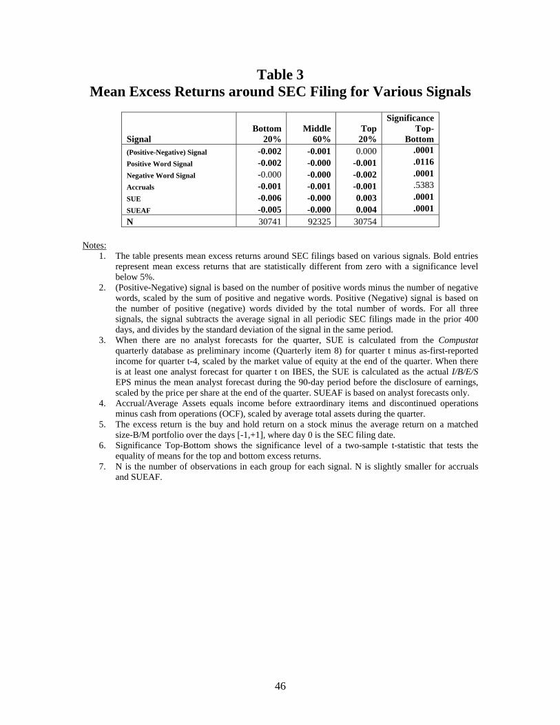
Table 3 Mean Excess Returns around SEC Filing for Various Signals

Signal Bottom

20% Middle

60% Top

20%

Significance Top-

Bottom (Positive-Negative) Signal -0.002 -0.001 0.000 .0001 Positive Word Signal -0.002 -0.000 -0.001 .0116 Negative Word Signal -0.000 -0.000 -0.002 .0001 Accruals -0.001 -0.001 -0.001 .5383 SUE -0.006 -0.000 0.003 .0001 SUEAF -0.005 -0.000 0.004 .0001 N 30741 92325 30754

Notes:

1. The table presents mean excess returns around SEC filings based on various signals. Bold entries represent mean excess returns that are statistically different from zero with a significance level below 5%.


3. When there are no analyst forecasts for the quarter, SUE is calculated from the Compustat quarterly database as preliminary income (Quarterly item 8) for quarter t minus as-first-reported income for quarter t-4, scaled by the market value of equity at the end of the quarter. When there is at least one analyst forecast for quarter t on IBES, the SUE is calculated as the actual I/B/E/S EPS minus the mean analyst forecast during the 90-day period before the disclosure of earnings, scaled by the price per share at the end of the quarter. SUEAF is based on analyst forecasts only.

4. Accrual/Average Assets equals income before extraordinary items and discontinued operations minus cash from operations (OCF), scaled by average total assets during the quarter.

5. The excess return is the buy and hold return on a stock minus the average return on a matched size-B/M portfolio over the days [-1,+1], where day 0 is the SEC filing date.

6. Significance Top-Bottom shows the significance level of a two-sample t-statistic that tests the equality of means for the top and bottom excess returns.

7. N is the number of observations in each group for each signal. N is slightly smaller for accruals and SUEAF.

46

Table 4 Correlations among Regression Variables

BHR-Drift

BHR - Filing Accrual SUEAF SUE

(POS-NEG) POS

BHR - Filing -0.003 Accrual -0.040 0.001 SUEAF 0.043 0.053 0.025 SUE 0.060 0.061 0.062 0.947 (POS-NEG) 0.014 0.013 -0.001 0.059 0.072 POS 0.006 0.006 -0.047 0.018 0.014 0.520 NEG -0.080 -0.013 -0.045 -0.060 -0.082 -0.658 0.003

Notes: 1. The table presents Pearson correlations between regression variables, which include excess buy

and hold returns (BHR) on scaled signal ranks. Each signal is assigned its quintile rank, is divided by 4, and 0.5 is subtracted to obtain the scaled signal rank. The table is based on all available observations. Bold entries represent correlations that are statistically different from zero with a significance level below 5%.



4. Accruals/Average Assets equal income before extraordinary items and discontinued operations minus cash from operations (OCF), scaled by average total assets during the quarter.

5. BHR-Filing is the buy and hold return on a stock minus the average return on a matched size-B/M portfolio over the days [-1,+1], where day 0 is the SEC filing date. BHR-Drift is the excess BHR over the period from two days after SEC filing through one day after the preliminary earnings announcement in the subsequent quarter.

47

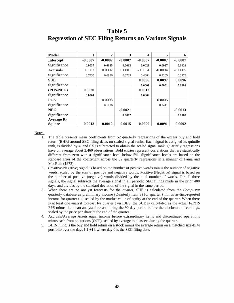
Table 5 Regression of SEC Filing Returns on Various Signals

Model 1 2 3 4 5 6 Intercept -0.0007 -0.0007 -0.0007 -0.0007 -0.0007 -0.0007 Significance 0.0037 0.0035 0.0033 0.0029 0.0027 0.0026 Accruals 0.0002 0.0002 0.0001 -0.0004 -0.0004 -0.0005 Significance 0.7435 0.6986 0.8739 0.4064 0.4265 0.3373 SUE 0.0096 0.0097 0.0096 Significance 0.0001 0.0001 0.0001 (POS-NEG) 0.0020 0.0013 Significance 0.0001 0.0064 POS 0.0008 0.0006 Significance 0.1206 0.2441 NEG -0.0021 -0.0013 Significance 0.0002 0.0060 Average R-Square 0.0013 0.0012 0.0015 0.0090 0.0091 0.0092

Notes:

1. The table presents mean coefficients from 52 quarterly regressions of the excess buy and hold return (BHR) around SEC filing dates on scaled signal ranks. Each signal is assigned its quintile rank, is divided by 4, and 0.5 is subtracted to obtain the scaled signal rank. Quarterly regressions have on average about 2,460 observations. Bold entries represent correlations that are statistically different from zero with a significance level below 5%. Significance levels are based on the standard error of the coefficient across the 52 quarterly regressions in a manner of Fama and MacBeth (1973).


3. When there are no analyst forecasts for the quarter, SUE is calculated from the Compustat quarterly database as preliminary income (Quarterly item 8) for quarter t minus as-first-reported income for quarter t-4, scaled by the market value of equity at the end of the quarter. When there is at least one analyst forecast for quarter t on IBES, the SUE is calculated as the actual I/B/E/S EPS minus the mean analyst forecast during the 90-day period before the disclosure of earnings, scaled by the price per share at the end of the quarter.


5. BHR-Filing is the buy and hold return on a stock minus the average return on a matched size-B/M portfolio over the days [-1,+1], where day 0 is the SEC filing date.

48

Table 6 Mean Excess Drift Returns for Various Signals

Signal Bottom

20% Middle

60% Top

20%

Significance Top-

Bottom (Positive-Negative) Signal -0.003 0.000 0.004 .0001 Positive Word Signal -0.001 0.000 -0.003 .0210 Negative Word Signal 0.003 0.000 -0.001 .0164 Accruals 0.012 0.001 -0.011 .0001 SUE -0.015 -0.001 0.020 .0001 SUEAF -0.009 -0.002 0.015 .0001 N 30741 92325 30754

Notes:

1. The table presents mean excess returns from two days after the SEC filing through one day after the subsequent preliminary earnings announcement for sub-groups based on various signals. Bold entries represent mean excess returns that are statistically different from zero with a significance level below 5%.




5. The excess return is the buy and hold return on a stock minus the average return on a matched size-B/M portfolio from two days after the SEC filing date through one day after the subsequent quarter’s preliminary earnings announcement.

6. Significance Top-Bottom shows the significance level of a two-sample t-statistic that tests the equality of means for the top and bottom excess returns.

7. N is the number of observations in each group for each signal. N is slightly smaller for accruals and SUEAF.

49

Table 7 Regression of Drift Excess Returns on Various Signals

Signal Intercept Accruals SUE Tone LOGMKT LOGPRICE NFORE RVOL RSQ

(Pos-Neg) -0.0092 -0.0263 0.0344 0.0060 -0.0023 0.0079 0.0002 0.0005 0.0300 Significance 0.2029 0.0001 0.0001 0.0020 0.0725 0.0329 0.4739 0.9708 0.0001

Pos -0.0092 -0.0260 0.0348 0.0043 -0.0023 0.0080 0.0002 0.0005 0.0301 Significance 0.2064 0.0001 0.0001 0.0542 0.0657 0.0313 0.4562 0.9565 0.0001

Neg -0.0093 -0.0264 0.0346 -0.0020 -0.0022 0.0078 0.0002 0.0007 0.0300 Significance 0.2007 0.0001 0.0001 0.3154 0.0736 0.0326 0.4994 0.3613 0.0001

Notes:

1. The table presents mean coefficients from 52 quarterly regressions of the excess buy and hold drift return on scaled signal ranks. Each signal is assigned its quintile rank, is divided by 4, and 0.5 is subtracted to obtain the scaled signal rank. Quarterly regressions have on average about 2,460 observations. Bold entries represent correlations that are statistically different from zero with a significance level below 5%. Significance levels are based on the standard error of the coefficient across the 52 quarterly regressions in a manner of Fama and MacBeth (1973).

2. Tone represents the tone change signal. (Positive-Negative) signal is based on the number of positive words minus the number of negative words, scaled by the sum of positive and negative words. Positive (Negative) signal is based on the number of positive (negative) words divided by the total number of words. For all three signals, the signal subtracts the average signal in all periodic SEC filings made in the prior 400 days, and divides by the standard deviation of the signal in the same period.



5. The excess drift return is the buy and hold return on a stock minus the average return on a matched size-B/M portfolio from two days after the SEC filing date through one day after the subsequent quarter’s preliminary earnings announcement.

6. LOGMKT is the log of market value of equity at quarter-end. 7. LOGPRICE is the log of price per share at quarter-end. 8. NFORE is the number of quarterly analyst forecasts. 9. RVOL is the ratio of traded shares in the 60 days prior to filing, scaled by number of shares

outstanding one day before filing.

50

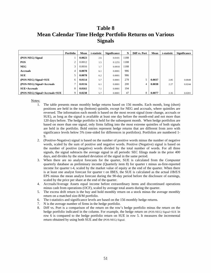
Table 8 Mean Calendar Time Hedge Portfolio Returns on Various

Signals

Portfolio Mean t-statistic Significance N Diff vs. Port Mean t-statistic Significance

(POS-NEG) Signal 1 0.0023 2.6 0.0101 1188 POS 2 0.0012 1.5 0.1255 1188 NEG 3 0.0016 1.7 0.0918 1188 Accruals 4 0.0078 6.1 0.0001 986 SUE 5 0.0078 6.2 0.0001 986 (POS-NEG) Signal+SUE 6 0.0114 5.7 0.0001 278 5 0.0037 2.85 0.0049

(POS-NEG) Signal+Accruals 7 0.0116 6.1 0.0001 200 4 0.0038 2.27 0.0244

SUE+Accruals 8 0.0161 7.1 0.0001 194

(POS-NEG) Signal+Accruals+SUE 9 0.0238 5.7 0.0001 47 8 0.0077 2.35 0.0201 Notes:

1. The table presents mean monthly hedge returns based on 156 months. Each month, long (short) positions are held in the top (bottom) quintile, except for NEG and accruals, where quintiles are reversed. The information each month is based on the most recent signal (tone change, accruals or SUE), as long as the signal is available at least one day before the month-end and not more than 120 days before. The hedge portfolio is held for the subsequent month. When hedge portfolios are based on more than one signal, only firms falling into the most extreme quintiles of both signals are held in the portfolio. Bold entries represent hedge returns that are different from zero with significance levels below 5% (one-sided for differences in portfolios). Portfolios are numbered 1-9.




5. The excess drift return is the buy and hold monthly return on a stock minus the average monthly return on a matched size-B/M portfolio.

6. The t-statistics and significance levels are based on the 156 monthly hedge returns. 7. N is the average number of firms in the hedge portfolio. 8. Diff vs. Port is a comparison of the return on the row’s hedge portfolio minus the return on the

hedge portfolio indicated in the column. For example, the hedge return on (POS-NEG) Signal+SUE in row 6 is compared to the hedge portfolio return on SUE in row 5. It measures the incremental return obtained by using both SUE and the (POS-NEG) Signal.

51

Table 9 Regressions of Calendar Time Hedge Portfolio Raw Returns

on Fama-French Factors

Hedge Portfolio Intercept Market SMB HML Momentum SUE 0.0088 -0.0826 0.0306 -0.0006 -0.009 t-statistic 6.03 -2.15 0.79 -0.01 -0.33 Accruals 0.0083 -0.0324 -0.0934 -0.105 -0.009 t-statistic 5.8 -0.85 -2.44 -2.14 -0.36 (Pos-Neg) 0.0021 0.0105 -0.0069 -0.03596 0.0061 t-statistic 2.14 0.4 -0.26 -1.07 0.33 Pos 0.0007 0.0500 -0.0472 -0.0311 0.0200 t-statistic 0.78 2.1 -1.97 -1.02 1.19 Neg 0.0017 -0.0252 0.0307 -0.0186 0.0097 t-statistic 1.55 -0.88 1.07 -0.51 0.48 SUE+(Pos-Neg) 0.0124 -0.0755 0.0061 -0.0326 -0.0233 t-statistic 5.34 -1.23 0.1 -0.42 -0.54 Accruals+(Pos-Neg) 0.0127 -0.0765 -0.044 -0.159 -0.0019 t-statistic 6.03 -1.38 -0.79 -2.23 -0.05 SUE+Accruals+(Pos-Neg) 0.0228 0.0587 -0.192 -0.134 0.0118 t-statistic 4.98 0.49 -1.58 -0.87 0.14

Notes:

1. The table presents regressions of monthly hedge raw returns on the Fama & French 3-factors plus momentum, taken from Kenneth French’s Data Library for the 156 months in our calendar time tests. Each month, long (short) positions are held in the top (bottom) quintile, except for NEG and accruals, where quintiles are reversed. The information each month is based on the most recent signal (tone change, accruals or SUE), as long as the signal is available at least one day before the month-end and not more than 120 days before. The hedge portfolio is held for the subsequent month. When hedge portfolios are based on more than one signal, only firms falling into the most extreme quintiles of both signals are held in the portfolio. Bold entries represent regression coefficients that are different from zero with significance levels below 5%.




5. The drift return is the monthly buy and hold return on a stock. 6. Market, SMB, HML and Momentum are regression coefficients of the raw hedge portfolio returns

on the Fama & French factors taken from Kenneth French’s Data Library.

52

Table 10 Regression of SEC Filing and Drift Returns on Various Signals

Information Environment Analysis

Panel A - Filing Returns Intercept Accrual SUE (Pos-Neg) D Acc*D SUE*D (Pos-Neg)*D N RSQ D=Size -0.0014 -0.0006 0.0118 0.0017 0.0013 0.0003 -0.0058 -0.0010 2449 0.0120 Significance 0.0002 0.3898 0.0001 0.0153 0.0039 0.6805 0.0001 0.2919 0.0001 D=B/M -0.0008 0.0001 0.0089 0.0003 0.0002 -0.0013 0.0011 0.0022 2449 0.0112 Significance 0.0090 0.8821 0.0001 0.6562 0.6989 0.1501 0.1985 0.0095 0.0001 D=Number of Analysts -0.0014 0.0005 0.0109 0.0023 0.0013 -0.0018 -0.0038 -0.0021 2449 0.0123 Significance 0.0001 0.5118 0.0001 0.0028 0.0200 0.0704 0.0009 0.0477 0.0001 Panel B - Drift Returns Intercept Accrual SUE (Pos-Neg) D Acc*D SUE*D (Pos-Neg)*D N RSQ D=Size 0.0010 -0.0270 0.0456 0.0062 -0.0007 0.0038 -0.0267 -0.0015 2449 0.0136 Significance 0.6881 0.0001 0.0001 0.0336 0.7359 0.3163 0.0001 0.6731 0.0001 D=B/M 0.0019 -0.0265 0.0363 0.0045 -0.0027 0.0040 -0.0016 0.0026 2449 0.0123 Significance 0.4300 0.0001 0.0001 0.0825 0.4081 0.3203 0.6906 0.4293 0.0001 D=Number of Analysts 0.0020 -0.0227 0.0420 0.0059 -0.0022 -0.0049 -0.0185 0.0000 2449 0.0153 Significance 0.4802 0.0001 0.0001 0.0459 0.4857 0.1834 0.0004 0.9965 0.0001

Notes: 1. The table presents mean coefficients from 52 quarterly regressions of the excess buy and hold

return (BHR) around SEC filing dates and drift returns from two days after the SEC filing through the next earnings announcement on scaled signal ranks. Each signal is assigned its quintile rank, is divided by 4, and 0.5 is subtracted to obtain the scaled signal rank. Quarterly regressions have on average N observations. Bold entries represent correlations that are statistically different from zero with a significance level below 5%. Significance levels are based on the standard error of the coefficient across the 52 quarterly regressions in a manner of Fama and MacBeth (1973).

2. (Positive-Negative) signal is based on the number of positive words minus the number of negative words, scaled by the sum of positive and negative words. The signal subtracts the average signal in all periodic SEC filings made in the prior 400 days, and divides by the standard deviation of the signal in the same period.



5. D is a dummy variable which is equal to one if the partitioning variable is above its cross-sectional quarterly median. The dummy variables are size, the market value of equity at quarter-end, the book/market ratio (B/M), and the number of analysts.

53

Table 11 Regression of SUE at Quarter t+1 on SUE at Quarter t and

Tone Signals

Signal Intercept SUE Size Accrual B/M NFORE Price Signal N R-Sq

SUE 0.0012 0.0861 0.0000 -0.0026 -0.0035 0.0000 0.0000 2259 0.0358 Significance 0.3226 0.0001 0.8381 0.5156 0.0001 0.0315 0.0239 0.0001

(Pos-Neg) 0.0012 0.0857 0.0000 -0.0025 -0.0035 0.0000 0.0000 0.0008 2259 0.0366 Significance 0.3103 0.0001 0.8696 0.5274 0.0001 0.0645 0.0245 0.0001 0.0001

Pos 0.0012 0.0860 0.0000 -0.0026 -0.0035 0.0000 0.0000 0.0002 2259 0.0362 Significance 0.3347 0.0001 0.8138 0.5260 0.0001 0.0340 0.0239 0.1323 0.0001

Neg 0.0012 0.0853 0.0000 -0.0032 -0.0035 0.0000 0.0000 -0.0010 2259 0.0369 Significance 0.3139 0.0001 0.8833 0.4282 0.0002 0.0501 0.0245 0.0001 0.0001

Notes:

1. The table presents mean coefficients from 51 quarterly regressions of the earnings surprise in quarter t+1 on the earnings surprise in quarter t, several control variables, and the tone change signals. Bold entries represent correlations that are statistically different from zero with a significance level below 5%. Significance levels are based on the standard error of the coefficient across the 51 quarterly regressions in a manner of Fama and MacBeth (1973).



4. Size is market value of equity at quarter end. Accruals/Average Assets equals income before extraordinary items and discontinued operations minus cash from operations (OCF), scaled by average total assets during the quarter. B/M is the ratio of book to market value of equity at quarter-end. NFORE is the number of quarterly earnings forecasts in the 90-day period prior to the earnings announcement. Price is price per share at quarter-end.

5. N (R-Sq) is the average number of firms (R-Square) in the quarterly cross-sectional regressions.

54

Table 12 Mean Excess Returns for Signal Combinations

Filing Returns

Low Tone Medium

High Tone

High-Low

Negative Surprise -0.005 -0.004 -0.003 0.002 N 12414 32228 9627 Positive Surprise 0.000 0.001 0.002 0.002 N 18327 60097 21127 Drift Returns

Low Tone Medium

High Tone

High-Low

Negative Surprise -0.014 -0.012 -0.011 0.003 N 12414 32228 9627 Positive Surprise 0.005 0.007 0.010 0.005 N 18327 60097 21127 Low Accruals (20%) 0.006 0.012 0.017 0.011 N 5180 15136 5284 Medium Accruals (60%) -0.001 0.001 0.003 0.004 N 15626 46020 15258 High Accruals (20%) -0.016 -0.011 -0.005 0.011 N 5207 14989 5421

Notes:

1. The table presents mean 3-day excess returns centered on the SEC filing date (Filing Returns) and mean excess returns from two days after the SEC filing through one day after the subsequent preliminary earnings announcement (Drift returns) for combinations of signals.

2. Tone is based on the (Positive-Negative) signal, the number of positive words minus the number of negative words, scaled by the sum of positive and negative words. The signal subtracts the average signal in all SEC filings made in the prior 400 days, and divides by the standard deviation of the signal in the same period.

3. When there are no analyst forecasts for the quarter, SUE is calculated from the Compustat quarterly database as preliminary income (Quarterly item 8) for quarter t minus as-first-reported income for quarter t-4, scaled by the market value of equity at the end of the quarter. When there is at least one analyst forecast for quarter t on IBES, the SUE is calculated as the actual I/B/E/S EPS minus the mean analyst forecast during the 90-day period before the disclosure of earnings, scaled by the price per share at the end of the quarter. Positive and negative surprise is based on the sign of SUE.

4. Accruals equal income before extraordinary items and discontinued operations minus cash from operations, scaled by average total assets during the quarter.

5. The excess return is the buy and hold return on a stock minus the average return on a matched size-B/M portfolio from two days after the SEC filing date through one day after the subsequent quarter’s preliminary earnings announcement.

6. High (Low) tone is the extreme high (low) 20%. High-Low represents the mean High tone return minus the mean Low tone return.

7. N is the number of observations and is provided below the mean for each table entry.

55

management’s tone change, post earnings announcement drift ... · management’s tone change,...

Documents