underreaction, trading volume, and post-earnings announcement

Underreaction, Trading Volume,

and Post-Earnings Announcement Drift*

Wonseok Choi [email protected]

Department of Economics Harvard University

Jung-Wook Kim**

[email protected] School of Business

University of Alberta

First draft: April, 2001 This draft: November, 2001

ABSTRACT

In this paper, we develop a simple model in which trading volume contains information about future stock returns. Specifically, our model explains why high trading volume is observed when a firm announces earnings news and how trading volume can be related to the initial underreaction of the stock price. Our model has a clear testable implication that high abnormal trading volume predicts a stronger drift. We test our model’s implication and find strong evidence for the model in the case of positive news. Weaker evidence is found in the case of negative news. We also discuss possible explanations for the asymmetric informativeness of trading volume. JEL code: G14 Key words: Earnings announcement, Underreaction, Public information, Trading volume, Drift

* We especially thank Jeremy Stein, Andrei Shleifer, Rafael LaPorta for their suggestions and guidance. We also thank John Campbell, Randall Morck, Mark Huson, Jason Lee, Aditya Kaul and seminar participants at Harvard University and University of Alberta for helpful suggestions. Wonseok Choi acknowledges a scholarship from KFAS and Harvard-Yenching Institute, and Jung-Wook Kim acknowledges funding from POSCO. ** Corresponding author: 2-32C Business Building, University of Alberta, Edmonton, AB, Canada T6G 2R6. Tel) 780-492-7987 Fax) 780-492-3325. E-mail: [email protected]

1

1. Introduction

Ball and Brown (1968) are the first to find that the abnormal return of firms with

positive earnings news continues to drift upward after the earnings announcements and

that the opposite is true for firms with negative news. Since then, many researchers have

extensively investigated the post-earnings announcement drift. Bernard (1993) writes an

excellent survey paper dealing with the underreaction of stock prices to announcements

of companies’ earnings. He conjectures that market participants do not recognize the

positive autocorrelations in earnings changes but in fact believe that earnings follow a

random walk. In this case, investors do not fully reflect the news content of earnings

announcements and a subsequent drift can be observed. Recently, there have been several

attempts to explain investors' underreaction.1 Barberis, Shleifer and Vishny (1998,

henceforth BSV) provide a formal model to explain underreaction to earnings

announcements.2 Their explanation of underreaction to earnings announcements is

related to investors’ conservatism. Conservatism refers to the reluctance of individuals to

update their beliefs upon receiving new information (Edwards, 1968). Conservatism fits

the underreaction story very well. Investors subject to conservatism might disregard the

full information content of an earnings (or some other public) announcement because

they tend to cling, at least partially, to their prior estimates of earnings rather than update

their estimates based on the new information contained in the earnings announcement.

Daniel, Hirshleifer, and Subrahmanyam (1998, henceforth DHS) show that when

investors overestimate the precision of private signals, they can generate an initial price

reaction that is weaker than the fully rational one. In their model, investors do not react

much to public signals when the content of the new information conflicts with their

2

private signals.3 Hong and Stein (1999, henceforth HS) provide a model in which private

information diffuses slowly. In their model, “newswatchers” fail to form sophisticated

forecasts of future stock prices since they make forecasts based only on private signals

they observe and do not condition their estimates on past or current prices. In this case,

stock prices will exhibit momentum. HS also explain how their model could generate

underreaction to public information. Although the news announcement itself is public, it

may require other private information (e.g., knowledge of the stochastic processes

governing earnings) to convert the news into a judgment about value.

In this paper, we try to capture the degree of underreaction of stock prices and its

effect on the magnitude of the drift after earnings announcements by looking at trading

volume. We pay attention to the fact that abnormally high trading volume, unrelated to

the magnitude of price changes, is generated around earnings announcements. Kandel

and Pearson (1995) show that even when there is little price change, a considerable

amount of abnormal trading volume exists around earnings announcements. They

interpret this as evidence of the existence of heterogeneity among investors in

interpreting the content of earnings announcement news. We fully agree with their

assessment, but we go one step further and investigate the sources of differences in

investor interpretations and their implications on drift patterns.

This paper assumes heterogeneity in the belief-updating processes among investors.

The assumption of heterogeneity in investors’ beliefs is not new, and in fact we have a

variety of theoretical and empirical evidence that supports this hypothesis. Kim and

Verrecchia (1993) develop a model in which the precision of pre-announcement public

and private information affects trading volume. Kandel and Pearson (1995) suggest a

3

model of differential interpretations of public information. Harris and Raviv (1993) also

suggest a similar model in which investors disagree on the importance of public news. In

the psychological literature, Griffin and Tversky (1992) suggest that the experts and the

novices may react differently to new evidence.

In our model, we assume two types of investors. The first type of investors is fully

rational in the sense that they follow Bayes’ rule in updating their posterior beliefs. The

second type of investors is those who put irrationally low weight on news. We show that

the degree of underreaction can be captured by the weight these investors put on news

and that the weight can be recovered from trading volume data.

In this case, trading volume can arise as a result of the interaction between these two

groups of investors; moreover, it has informative implications for the subsequent drift

pattern. As the weight that the second type of investors puts on news decreases (i.e., the

more conservative investors become), we observe higher trading volume as a result of the

interaction between the two types of investors, and the initial price reaction to earnings

announcements should be less than the rational level (i.e., the level when there are no

underreacting investors). Consequently, there should be a subsequent price adjustment

(drift) following an earnings announcement when the initial price reaction does not fully

reflect the information contained in the earnings announcement. Since rational-level price

change is unobservable, only by looking at the trading volume could we infer whether

price underreacts to news or not. This is the unique role of trading volume in our paper.

In our model, we focus on the “news characteristics” of earnings announcements as

a determinant of the degree of underreaction. To understand this statement, consider two

firms that share the same firm characteristics (e.g., market capitalization, institutional

4

ownership, analyst coverage). Even though the two firms’ announcements generate the

same magnitude of surprise in terms of standardized unexpected earnings (SUE), the

reaction of investors might differ depending on the characteristics of the news. If the

value implication of the news is really clear, the weight that the second type of investors

places on the news will converge to the rational level and there will not be much trading

volume. However, if the content of the news is murky at best, the same level of earnings-

surprise would generate much higher trading volume and price will not rise as much as in

the previous case where the information content is clear.

In other words, we argue that the magnitude of conservatism could depend on the

news characteristics and that might be well captured by abnormal trading volume. In our

empirical work, we carefully proceed to measure abnormal trading volume that is not

correlated with firm characteristics and depends only on the news characteristics. A

similar argument can be found in Klibanoff, Lamont, and Wizman (1998). They test the

behavioral hypothesis that investors underreact less to news that is salient. They test

investors’ reaction to salient news in closed-end country funds and measure saliency by

the appearance on the front page of The New York Times. They find that the price of a

closed-end country fund reacts more strongly to news about its fundamentals when the

country whose stocks the fund holds appears on the front page of the newspaper.

Our paper also contributes to research on understanding what information trading

volume contains in addition to the information that is contained in the return data. Blume,

Easley and O’Hara (1994) show that information quality that can not be deduced from

price statistics can be inferred from trading volume data. In this paper, we argue that

5

trading volume can generate additional information about future stock returns since it

captures the degree of clarity of information4 contained in earnings announcements.

Our research stands out from the others in the literature that investigates volume and

return relationships in that we focus specifically on an informational event. Some papers

look at trading volume and return relationships when there is no information asymmetry

(e.g., Campbell, Grossman, and Wang (1993) and Conrad, Hameed, and Niden (1992)),

while others look at trading volume and return autocorrelation patterns in relation to

information asymmetry due to the existence of private information (Llorente, Michaely,

Saar and Wang (2000)). Recently Swaminathan and Lee (1999, 2000) investigate trading

volume and earnings announcements but in a different context. They look at the

implications of past trading volume for price momentum.5 Gervais, Kaniel, and

Mingelgrin (2001) find that stocks experiencing unusually high trading volume over a

day or a weekend tend to appreciate over the course of the following month. They argue

that trading volume could be a good proxy for the level of investors’ interest in the stock

and thus the visibility of the stock captured by trading volume could explain future stock

returns quite well. Pritamani and Singal (2001) investigate return dynamics when firms

experience extremely large price changes around several corporate events. They find that

subsequent returns move in the same direction as the initial price changes when large

price change is accompanied by large trading volume. Our study differs from theirs in

that we do not confine our sample to firms that experience extremely large price changes.

We look at all NYSE and AMEX firms that made earnings announcements during

the 1988-1996 period to test our model’s prediction.6 We develop a measure of volume

that is not correlated with the magnitude of the initial price reaction to the news and firm

6

characteristics. This measure of volume is defined as the residual from the cross-sectional

regression of volume on price changes and firm characteristics. We find that in the cases

of positive news, our model’s prediction is strongly supported in every specification we

use to calculate the residual volume. High (low) residual volume that is generated due to

an earnings announcement implies a stronger (weaker) drift. However, we could find

only weak evidence for the relationship between abnormal trading volume and the

subsequent drift for the cases of negative news (the results vary somewhat depending on,

for example, which surprise measure we use). This asymmetry in itself is interesting to

note. We conjecture that the weak evidence for the informativeness of trading volume for

future drifts may be due to institutional arrangements that our model cannot capture, e.g.,

short-sales constraints. For instance, some institutional investors, such as mutual funds,

do not usually take short positions. In this case, the low residual volume we calculate

may not be due to news characteristics but due to the restriction that some investors must

sit back from the trading scene because of the short-sales constraint. Thus for negative

news, the residual volume we calculate is subject to additional noise relative to the one

we calculate for positive news and it may not serve its purpose well as a predictor of drift.

Diamond and Verrecchia (1987) and Chen, Hong, and Stein (2000) look at the

implications of short-sales constraints for stock returns in relation to private information.

The paper is structured as follows. Section 2 presents a model that shows how

trading volume could be a good proxy (after necessary adjustments) for news

characteristics that are crucial to investors’ underreaction. Section 3 and 4 contain our

main empirical results on the relationship between trading volume and drift. Section 5

concludes.

7

2. Conceptual framework

2.1. Model

We make the following assumptions7.

(1) There are two kinds of assets: a riskless asset with a zero rate of return, and a risky

asset with an uncertain payoff R. The supply of the risky asset is normalized at 0.

(2) There are three time periods. At time 1, investors have access to pre-disclosure

information about the firm, and form symmetric prior beliefs about R. At time 1, the

symmetric prior belief of investors is represented by a normal density with mean X and

precision Z.

(3) At time 2, a public signal is announced, and investors update their beliefs. The public

signal at time 2 is given by , where is normally distributed with mean zero

and precision b. Here the precision parameter b can be interpreted as the informativeness

of the public signal about the stock's future value. At time 3, R is realized, and investors

consume their wealth.

ε+= RL ε

(4) There are two types of investors indexed by i=1, 2, depending on how they react to

earnings news. The first type of investors, whose proportion is α , is the underreacting

investors. Their perceived precision of the public signal is lower than the true precision,

but the extent to which the perceived precision diverges from the true precision depends

on the saliency of the public news. The assumption that the perceived precision is lower

than the true precision reflects the psychological evidence that individuals update their

posterior beliefs too little relative to the rational Bayesian benchmark. This type of

investors underestimates the degree to which the public news is correlated with the future

8

firm value, and puts too much weight on their prior beliefs. We assume that the

perceived precision of the public signal to the first type of investors is ω , where ω

and ω increases with the saliency of the news. Thus if the content of the news is clear (or

salient) enough, ω is close to 1 and even the first type of investors will behave as if they

were fully rational Bayesian investors who perceive the precision of the public

information correctly as b .

b⋅ 1≤

(5) The second type of investors, whose proportion is 1 , is rational in the sense that

their perceived precision equals the true precision of the public signal. They have the

ability to correctly interpret the importance of the public news for the stock's future value.

This type of investors can be thought of as risk-averse arbitrageurs who are free from the

psychological biases mentioned above. After the public signal is revealed, they update

their beliefs in a correct way according to Bayes’ rule.

α−

(6) All investors maximize the expected utility of third-period wealth. The utility function

takes on the exponential form, U WeW −−=)( .

A. Time 1

All investors choose their demands (m) of the risky asset to maximize their expected

utility of the third-period wealth.

) )](exp[ ( max 11 PRmEm

−⋅−− (1)

where represents expectation with respect to the prior belief of investors. is

the first-period price. The resulting demand for the risky asset can be represented as

follows:

)(1 ⋅E 1P

ZPXm ⋅−= )( 1 (2)

9

Using the market equilibrium condition, we can calculate the first-period equilibrium

price.

XP =1 (3)

The first-period equilibrium price is equal to the mean of the prior belief distribution

of investors.

B. Time 2

After the public signal is revealed, investors update their beliefs, and the second

round of trading occurs. The posterior belief of the rational investors is given by a normal

density with mean Y , where Y can be expressed as follows: 2 2

LXLREY ⋅−+⋅== )1()( 22222 ρρ (4)

Here )(2 bZZ +=ρ denotes the relative weight put on the prior belief by the

rational investors. Precision of the posterior belief is . represents the

expectation with respect to the information set of the second type of investors at time 2.

bZ + )(22 ⋅E

The mean Y of the posterior belief of the underreacting investors is given by the

following:

1

bZZ

LXLREY

⋅+=

⋅−+⋅==

ωρ

ρρ

1

11121

where

)1()( (5)

In equation (5), ω is the parameter of importance. This is the parameter that will

determine the degree of underreaction in the model. It is important to note that ω

represents news characteristics. As the saliency of the news becomes lower, ω decreases

and the underreacting investors put less weight on public signals in updating their beliefs.

10

We can see that the weight the underreacting investors put on their prior belief,

bZZ

⋅+=

ωρ1 , is greater than that of the rational investors. In brief, the underreacting

investors are overconfident about their prior beliefs.

The equilibrium price will be determined by the interaction of these two types of

investors and can be calculated as follows:

bbbZ

bLXZP ⋅+⋅=+

⋅+⋅= ])-(1[ˆ where,ˆ

ˆ2 αωα (6)

When we compare , it can be shown that the price change between the two

periods is linearly related to the surprise component of the public signal.

21 and PP

XLLELSurprise

SurprisebZ

bPPP

−=−=

⋅+

=−=∆

)(ˆ

ˆ

1

12 (7)

If the content of the news is so clear as to make even the first type of investors

behave as if they were rational investors, the price change would be

SurprisebZ

bPPP ⋅+

=−=∆ 12 (8)

Since bZ

bbZ

bˆ

ˆ

+≥

+, the price change in response to public news is less than the

fully rational level.

Equation (7) shows that as the saliency of the public news becomes lower (so ω

becomes lower), the underreacting investors will underestimate the importance of the

earnings news by more, the weighted average of the perceived precision of the public

signal ( ) becomes lower than the true precision (b ), and therefore the price change in b̂

11

reaction to the news will be less than the rational level. If the post-announcement drift

emerges as an adjustment process due to an irrationally small initial price reaction to the

news, the lower saliency of the news will lead to a greater magnitude of the drift

afterwards.

However, there is no way to quantitatively measure the saliency of news by looking

at the price change alone since we cannot infer the amount by which the initial price

reaction differs from the fully rational level. But trading volume around an earnings

announcement can help us make this inference.

Trading volume in reaction to the public signal would be the absolute value of the

change in the holdings of one type of investors and can be expressed as follows:

)1

1(

1)1(α

ω

αα−

−

⋅⋅−⋅∆= ZPVolume (9)

In equation (9), we can see that as ω increases (i.e., the news is more salient),

trading volume will be lower for a given magnitude of the price change. When the public

news is more salient, the underreacting investors incorporate more of the information

content of the news into their posterior beliefs, and therefore, the difference in the

interpretation of the public news between the rational investors and the underreacting

investors becomes smaller, hence leading to low trading volume. At the extreme, if ω =1,

then all investors are updating their beliefs using the true precision and there will be no

trading volume. As the saliency of the news becomes lower, the difference in the

interpretation of the news between the two types of investors increases, and larger trading

volume will be induced.

12

When positive news is announced ( ), the price will fail to rise to the

fully rational level, and the underreacting investors, who do not update their beliefs in the

face of new evidence by as much as the rational investors, will have lower expectations

of the future stock value than the rational investors. Therefore underreacting investors

will try to sell stocks and rational investors will buy from them. On the other hand, when

negative news is announced ( ), the price will fail to go down to the fully

rational level, and the underreacting investors, who did not adjust their posterior beliefs

as much as the rational investors, will become buyers, and the rational investors will

become sellers.

0)(1 >− LEL

0<)(1− LEL

In equation (9), we can see that the trading volume is correlated with three

components. First, volume is positively correlated with the magnitude of the price change

as long as there exists some degree of differential interpretation about the news content.

Second, volume will also be influenced by the firm characteristics that are related to

the precision of pre-disclosure information (Z) and the proportion of rational investors

(1 ) among the firm’s clientele. α−

Last, trading volume is related to the degree of underreaction and the news

characteristics that influence it. Public news that has clear value implications for a stock,

such as the announcement of a takeover bid at a specific price, will induce lower trading

volume. But when it is not easy to interpret the content of the public news, the reaction of

the two types of investors differs and larger trading volume will be observed. Also, high

saliency of the news will reduce the degree of underreaction by the first type of investors.

Equation (9) is a very important benchmark for the empirical part of the paper.

Controlling for the price change and other firm characteristics that might be related to the

13

level of α and Z8, we can capture the part of the trading volume that is related to the news

characteristics and has drift implications.

2.2. Identifying the degree of underreaction

In our model, the price change is less than the rational level, due to the existence of

investors who do not give rational weight to the public news in updating their beliefs.

However, we are not able to identify the degree of underreaction by observing the price

change alone, because the true surprise component of the public news is unobservable

and the saliency of the news is not quantifiable. But we can infer the degree of

underreaction, , using the trading volume after controlling the price change and firm

characteristics. Suppose there are two firms with identical firm characteristics

( ). On the day of the earnings announcement, one firm

exhibits a 2% price change with zero volume. The other firm also exhibits a 2% price

change but with high volume. We can infer that the 2% change for the first firm is

rational in the sense that all investors were acting as Bayesian investors. For the second

firm, we can infer that the 2% change was less than rational, and therefore we will

observe further adjustment in the form of a (stronger) post-announcement drift.

ω

same Z and thetherefore α

So, our empirical strategy is to identify the firms that have exhibited abnormally high

trading volume after controlling for the magnitude of the price change and firm

characteristics, and to see if these firms exhibit a stronger drift. Controlling for the firm

characteristics is crucial in this context. In the world according to the model, we have to

control for firm characteristics to control for different levels of α and Z. In addition, in

reality, different firms may have different arbitrage capacities and trading costs just to

14

name two distinguishing differences. For example, Karpoff (1987) shows that trading

costs are one of the primary determinants of the level of trading volume. Lower trading

costs will lead to a larger volume reaction to news. The most natural way of controlling

for the price change and firm characteristics is to run a regression of volume on the

variables we want to control for, and use the residual volume as our measure. Our

regression specification will be developed in section 4.

3. Data and variables used in the study

3.1. Measure of surprise and drift

We obtain quarterly earnings announcement dates and earnings per share from

COMPUSTAT for the period between 1988 and 1996, and retrieve data on daily returns,

market capitalization, and daily trading volume (share turnover) from CRSP.

CDA/Spectrum provides the data on the percentage of firms’ shares held by institutions,

and IBES data contain the number of analysts who have made a forecast for each firm’s

quarterly earnings. We confine our sample to NYSE/AMEX firms following the

convention of the volume literature of not including NASDAQ firms.

We construct Standardized Unexpected Earnings (SUE) as a measure of surprise

following Bernard and Thomas (1993). SUE is defined as

))((

1

1

)(

ttt eEe

tttt

eEeSUE

−−

−−=

σ (10)

15

where denotes earnings announced at time t, is an expectation of those

earnings as of time t-1, and σ denotes the historical standard deviation of the difference

between quarterly earnings and their expectation.

te )(1 tt eE −

We will simply set , earnings in the same quarter a year ago, based on

the seasonal random walk. This measure of SUE assumes that investors expect this

quarter’s earnings to be the same as those of the same quarter last year. Bernard (1993)

has shown that even this simplistic measure of SUE is related to stock price reactions.

41 )( −− = ttt eeE

9

Another surprise measure we use for a robustness check is the cumulative abnormal

return (CAR) over the three-day period surrounding an earnings announcement. First, we

calculate size-matched abnormal return as in Bernard (1993) tir ,10, and sum the

abnormal returns over the three-day period surrounding an earnings announcement. Thus

if a firm makes an announcement at 0, the three-day CAR (henceforth TDC) is calculated

as the sum of abnormal returns of Day -1, 0 and 1.

∑−=

=1

1TDC

titi r (11)

This measure assumes that investors’ surprise is well captured by price changes

surrounding an earnings announcement.11

We define the post-announcement drift as the cumulative abnormal return (CAR) for

each portfolio for a certain period of time after the announcement, excluding the 3 days

16

surrounding the announcement. For example, a 30-day drift is CAR , where

and t=0 represents the announcement day

131 CAR−

∑=

=T

titT rCAR

0

12.

Table 1 reports the descriptive statistics of our sample. As in previous studies, we

can observe that there exists a post-announcement drift in the same direction as the price

change in the announcement window, no matter which measure of surprise we use.

Figure 1 presents the drift patterns in SUE quintiles and TDC quintiles. SUE quintiles are

based on the cutoff points in the distribution of SUEs in the previous quarter. TDC

quintiles are based on the cutoff points in the distribution of TDCs in the current quarter.

3.2. Calculating residual trading volume that captures ω

In this section, we carefully calculate residual trading volume that captures news

characteristics ω. Ideally, residual trading volume should not be correlated with the

magnitude of the price change and firm characteristics. In this case, the source of

variation in residual trading volume would only come from the news characteristics.

We proceed in two steps. The first step is to control for normal trading volume

outside event windows. Some firms are more actively traded than others. Some firms

move more closely with the market than others. To capture the part of volume generated

strictly by the arrival of news, we would like to control for differences in the intensity of

trading activity during normal periods and for market-wide effects. The second step is to

control for the part of the event trading volume that might be related to the magnitude of

the price change and firm characteristics within the event windows. Different firms can

17

have different levels of α and Z. We should control for this within the event window to

purge the part of trading volume that is due to firm characteristics.

3.2.1. First step

As the first step, we try to control for the normal level of trading volume outside

earnings announcement windows. For this purpose we try to obtain market-adjusted

trading volume. We calculate market-adjusted trading volume as follows. First, we

regress the firm's daily turnover (shares traded/shares outstanding) on the value-weighted

market turnover in the year prior to the announcement.13 Second, market-adjusted volume

for a given day is calculated by subtracting the predicted volume using the regression

from the actual volume.

kt iVMktTO

t-i ktiTO

VMktTOTO

itk

tk

titi

itk

itktktitiitk

day ,year in ,firmfor volumeadjusted-Market:novermarket tur weighted-Value:

1yearin firmfor modelmarket of estimatest Coefficien :,day ,year in , firmfor Turnover :

1,1,

1,1,

−−

−− ++=

βα

βα

(12)

Third, we sum the abnormal volumes in the three-day window. Market-adjusted

trading volume will be further refined in the next section to control for firm

characteristics and absolute price changes within the earnings announcement windows.

3.2.2. Volume, price change and firm characteristics

Before we move to the second step, we describe in this section the characteristics of

the reaction of market-adjusted volume to earnings announcement news. In Table 1, the

18

market-adjusted trading volume reaction is much greater when the news is positive, while

the magnitude of the price changes are similar in TDC quintiles 1 and 5. That is, when

the magnitude of price changes is the same, volume reaction is greater when the price

change is positive. This is consistent with previous studies (Karpoff 1987). This

asymmetry in the volume-return relationship has been explained by the existence of

short-sales constraints. When the news is negative, those who want to sell but are subject

to short-sales constraints cannot participate in the market (Chen, Hong, and Stein 2000).

So, short-sales constraints reduce the trading volume when the news is negative.

Short-sales constraints can be severe for smaller firms. To address this issue, Figure

2 reports the influence of firm size on market-adjusted volume reaction in each TDC

quintile. For the firms in size decile 1, the market-adjusted volume generated in TDC

quintile 1 is only a fourth of that in quintile 5. But this asymmetry gradually disappears as

the firm size increases. In size decile 10, market-adjusted volume reaction in TDC

quintiles 1 and 5 are fairly symmetric. Figure 3 reports the influence of institutional

ownership on market-adjusted trading volume in SUE and TDC quintiles. The effect of

institutional ownership seems to be similar to that of size.

As is clear in Figures 2 and 3, there clearly exists an asymmetry in the relationship

between volume and explanatory variables (magnitude of price changes, firm

characteristics) depending on whether the news is positive or negative. The trading

volume when there is negative news is significantly lower than when there is positive

news, and the effects of firm characteristics were significantly different, too. It should be

noted that in cases of negative news, the existence of short-sales constraints may make

19

our measure of volume a noisier signal of news characteristics that we intended to capture

in the second step.

3.2.3. Second step

Now we estimate a cross-sectional regression of trading volume on the price change

and firm characteristics to obtain a measure of residual trading volume that captures news

characteristics. There are 34 quarters in our sample period. We estimate cross-sectional

regressions for each quarter and report the means of each quarter’s coefficient estimates,

the t-statistics for the time-series of coefficient estimates, and the average of the adjusted

R-squares.

Specification 1 is our benchmark regression of market-adjusted volume on the

absolute value of the price change alone.14 To this specification, we will add several more

control variables that are supposed to capture firm characteristics. Our measure of the

price change is the CAR over the three-day announcement period (TDC).

tivP

t i V

vPV

ti

ti

ti

titittti

quarterin stock for volumeResidual :nt windowannounceme over the CAR of valueAbsolute :

quarter in stockfor volumeadjusted-Market :∆

+∆⋅+= βα

Table 2, Panel A (first row) reports the regressions results. First we estimate cross-

sectional regressions for each quarter without conditioning on a TDC quintile (Panel A).

To account for the possibility of a piecewise linear relationship between market-adjusted

trading volume and TDC, we also estimate quarterly cross-sectional regressions for each

TDC quintile (the first rows of Panel B and Panel C report regression results for quintiles

1 and 5). We have seen in the previous section that the relationship between volume and

20

the explanatory variables differs depending on whether the news is positive or negative.

Therefore, separate regressions by TDC quintiles seem a more appropriate way to

calculate residual volume. In the following section where the relationship between

residual volume and drift is reported, separate regressions by TDC quintiles will be used.

However, the results do not change significantly when we use residual trading volume

that is calculated using all TDC quintiles. In all Panels, the coefficient of the absolute

value of TDC turns out to be positive and significant. Adjusted R-squares range from

4.9% to 7.8%.

Specifications 2-8 are the regressions of market-adjusted volume on price changes

and other firm characteristics.

Specification 2 adds the price level in the regression.

[ Specification 2 ]

tivprice

Pt iV

vpricePV

ti

ti

ti

ti

titittittti

quarter in stock for volumeResidual :Price)Stock Log(1 :

nt windowannounceme over the CAR of valueAbsolute :quarter in stockfor volumeadjusted-Market :

21

+

∆

+⋅+∆⋅+= ββα

The motivation for including the price level is to control for differences in

transactions costs. If the price is higher, the bid-ask spread becomes smaller in terms of

the percentage of price and this could lead to greater volume reaction. It turns out that

this variable is positive and highly significant in all three Panels. The increase in the

adjusted R-square is the most dramatic in the case of Panel B, which looks at the first

TDC quintile (negative news). The adjusted R-square increases from 6.7% to 14.1%.

21

In specification 3, we include market capitalization (size) instead of the price level. It

turns out that larger firms have more trading. This is not surprising since a strong positive

correlation exists between size and price. However, the increase in the adjusted R-square

is much smaller, relative to its increase from specification 1 to specification 2. To check

the relative importance of the price level and size, we include both size and the price

level in specification 4.

[Specification 4]

tiv

P t iV

vSizepricePV

ti

ti

ti

titittittittti

quarter in stock for volumeResidual :Price)Stock Log(1 :Price

Log(Size):Sizent windowannounceme over the CAR of valueAbsolute :

quarterin stockfor volumeadjusted-Market :

ti

ti

321

+

∆

+⋅+⋅+∆⋅+= βββα

It is interesting to note that the adjusted R-square does not change much from that of

specification 2 (an increase of 0.1% to 0.3%) even though the coefficient estimates for

size are all significant. It is also interesting to note that the sign of coefficients of size

changes in Panels A and C when both size and the price are included. It remains positive

and marginally significant (t-statistic of 1.96) in the case of Panel B. Thus after

controlling for trading cost by including the price level, the independent contribution of

size could be negative.

In the next specification, we try to include institutional ownership and analyst

coverage in our regressions. It is possible that institutional investors are a proxy for

22

rational investors. It is also possible that analyst coverage affects the precision of pre-

announcement information. Care is needed, though, when including analyst coverage and

institutional ownership. It is known that the first size-quintile firms contain a number of

firms with no analyst coverage (Hong, Lim and Stein, 2000) and no institutional

ownership (Gompers and Metrick, 2000). This will bias the regression coefficients. Thus

when we include analyst coverage and institutional ownership, we discard the first size-

quintile. As a benchmark for the performance of specification 8, we re-estimate

specification 4 without the first size-quintile (specification 4*).

[Specification 8]

t ivAnIOSizeprice

Pt iV

vAnIOSizepricePV

ti

ti

ti

ti

ti

ti

ti

titittittijtittittti

quarter in stockfor volumeResidual :stock) thefollowing analysts ofNumber Log(1:

investors) nalinstitutioby held PercentageLog(1:Log(Size):

Price)Stock Log(1 :nt windowannounceme over the CAR of valueAbsolute :

quarter in stockfor volumeadjusted-Market :

54321

++

+

∆

+⋅+⋅+⋅+⋅+∆⋅+= βββββα

The adjusted R-square significantly increases when small firms are excluded in both

specifications 4* and 8. However, the levels of the adjusted R-square are basically the

same between specification 4* and specification 8 even though the added firm

characteristics, i.e., institutional ownership and analyst coverage, have significant

coefficient estimates.

We also estimate regressions for all specifications using raw trading volume instead

of market-adjusted trading volume. The basic results of Table 2 remain. In fact, whatever

23

specification we use for our residual trading volume measure, the main empirical results

of the paper change very little.

Our model's implication is that trading volume after controlling for the price change

and firm characteristics is related to the post-announcement drift. Thus ideally, residual

volume should not be correlated with the magnitude of the price change and firm

characteristics. Table 3 shows how well our regression specification controls for the price

change and firm characteristics. We form low/medium/high residual volume groups for

each TDC quintile and check whether residual trading volume is independent of other

firm characteristics and price changes. We can see that two residual-volume groups (low

and high) exhibit similar initial price reactions and firm characteristics, under all the

specifications used, while displaying a good spread in the market-adjusted volumes.

Figure 4 reports the means of the residual volume calculated using specification 4 in

50 cells sorted by size deciles and TDC quintiles. The results for the other specifications

are basically similar to those in this figure. In Figure 4, we can see that no visible pattern

exists in the relationship between residual volume and the initial price change or size. We

conclude that our residual volume measure calculated using cross-sectional regressions

has the desired property of no correlation with the initial price change and firm

characteristics, and that the differences in the drift between the high/low residual-volume

groups will well reflect the pure volume effect.

4. Empirical findings

4.1. Residual trading volume and drift patterns

24

Table 4 presents the relationship between residual volume calculated using

specification 2 (control variables: price change, log price) and the drift. We report drift

over 60 and 170 days after the announcement period. Table 4 shows the relationship

between residual volume and the drift in each SUE quintile. We also use our second

measure of surprise, which is TDC .

We find very strong evidence in support of our model’s prediction in the case of

positive news regardless of what surprise measure or what specification we use. High

residual trading volume firms exhibit a stronger drift than low residual trading volume

firms.

The results are much weaker when there is negative news. The results are somewhat

mixed depending on which surprise measure or horizon we use. In any case, we find

stronger results at the extreme quintiles, namely quintiles 1 and 5. This is not surprising

given Figure 2. The magnitude of market-adjusted trading volume is much greater in the

cases of these two quintiles compared to the other quintiles. Thus residual trading volume

can have more meaningful variation in these two quintiles.

Figure 5 clearly shows the drift patterns of high and low residual trading volume for

the first and fifth SUE and TDC quintiles. Regardless of which surprise measure we use,

quintile 5 (positive news) shows a clear drift pattern that depends on the magnitude of

residual trading volume. In the case of negative news, the drift pattern is consistent with

our model’s prediction when we use the SUE measure but the difference becomes

insignificant in the case of the TDC measure.

In SUE quintile 5, the high residual-volume group exhibits a significantly higher

drift than the low residual-volume group over all the horizons used. For Drift60, the drift

25

for a high residual-volume firm is 2.1% while that of a low residual-volume firm is

0.33%. The difference between the two is significant (t-statistic15 of 5.67). A similar

result is obtained at a longer horizon (Drift170: 2.23% vs. 0.62%, t-statistic for the

difference of the two is 2.47). The same pattern is observed in SUE quintile 4. For

Drift60, the drift for a high residual-volume firm is 1.32% while that of a low residual-

volume firm is –0.26%. The difference between the two is significant (t-statistic of 5.19).

A similar result is found at a longer horizon (Drift170: 1.46% vs. -0.25%, t-statistic of

2.68). It is very interesting to note that for the firms with positive news, the drift for low

residual-volume stocks is very weak. In the case of low residual-volume stocks, in the

fifth SUE quintile, the drift over 60 days is only 0.33%. The drift even becomes negative

(though not individually significant) for the fourth SUE quintile. This implies that the

unconditional drift we observe in Figure 1 is mainly driven by high residual-volume

firms. The basic results still hold even when we use TDC as our surprise measure. In

TDC quintile 5, the high residual-volume group exhibits a significantly higher drift over

all the horizons reported.

In SUE quintile 1, the difference in the drifts between the two residual-volume

groups is insignificant over the 60-day horizon, but the magnitude of the drift over 170

days is significantly higher for the high residual-volume group (-4.71% vs. -3.17%, t-

statistic of 2.12). However, we are cautious in concluding that our model’s prediction

also survives in the case of negative news since the relationship between residual volume

and the drift disappears when we use a different surprise measure, i.e., TDC. In TDC

quintile 1, there does not exist any statistically significant difference in drift patterns

26

between large and small residual trading volume firms. We will discuss the possible

explanation for the weak evidence in the case of negative news in section 4.3.

We also check whether we can get similar results for different specifications. Figure

6 reports the drift pattern when we calculate residual trading volume using specification

4. The pattern is almost identical to that of specification 2. We also report the results for

specification 8 where we include all the variables we consider in this paper. Here, when

we calculate residual trading volume, we discard the first size-quintile. Table 5 shows the

results under specification 8 for both surprise measures. The results of the previous

specifications still hold. When positive news arrives (SUE quintiles 4 and 5, or TDC

quintiles 4 and 5), the high residual-volume stocks exhibit a significantly higher drift than

the low residual-volume stocks. However, when there is negative news, the differences in

the drifts between the residual volume groups become insignificant at long horizons.

We have seen that the effect of high residual volume is to significantly increase the

magnitude of the drift when there is positive news. For positive-news stocks (quintile 5),

the effect of residual volume seems quite long-lived regardless of what surprise measure

or specification we use. The difference in the drifts between high and low residual-

volume stocks persists even up to 170 trading days after the announcement.

4.2. The magnitude of initial price reaction and residual trading volume

In this section, we further investigate the implication of the model. Our model

suggests that trading volume contains information about how much initial price reaction

differs from that of rational level. By looking at price change alone, we cannot identify

27

whether the price reaction around earnings announcement fully reflects the information

contained in the announcement or not. However, according to our theory, if a price

change is accompanied by large trading volume this is the case where price does not fully

reflect the information. In this case, we should expect stronger drift. We examine this

implication of the model in this section.

First, we test whether average reaction of price to earnings announcement is

different depending on the magnitude of residual trading volume. Our model predicts that

on average price reaction to a given SUE should be smaller for the group of firms that

experience high residual trading volume. To test this hypothesis we run the following

regression for the pooled sample.

itititit SUEVTDC εββα +++= ][ 21

where i denotes firm and t denotes the quarter when the announcement took place. Our

results are robust to whatever residual trading volume measure we use and we only report

the result where residual trading volume from specification 4 is used. If our model's

prediction is correct, we should have negative sign for since high residual trading

volume deters fully rational price reaction to the information. Also we run the following

regression.

2β

itititit SUEVDrift εγγα +++= ][ 21

28

Now dependent variable is our 60-day drift measure16 that does not include the

price change within the three-day window around earnings announcement. In this case

we expect to have positiveγ since stocks with high residual trading volume should

exhibit stronger drift. Table 6 reports the results. Panel A reports the coefficient estimates

and t-statistics when we use TDC as dependent variable. As expected the sign of is

negative and significant. Panel B reports the results when we use drift measure as

dependent variable. In this caseγ is positive and significant, which is consistent with the

model's prediction.

2

2β

2

To check the robustness of the results we run following quarterly regressions for

low and high residual-volume samples for each quarter.

ititit SUETDC εβα ++= 1

ititit SUEDrift εγα ++= 1

Thus we will have 34 coefficient estimates of and γ for each low and high

residual-volume sample. First, we test whether the means of are significantly different

between low and high residual-volume samples. Panel C shows that the mean of 's for

low residual-volume sample is significantly larger than that of high residual-volume

sample. Panel D reports the regression results when we use 60-day drift as the dependent

variable. In this case, the mean of γ for high residual-volume sample is significantly

larger than that of low residual-volume sample as expected.

1β 1

1β

1β

1

29

4.3. Asymmetry in informativeness of residual volume between positive and negative

news

We have seen that our model's prediction is strongly supported when positive news

is announced. However, when there is negative news, trading volume seems to have only

a weak, or insignificant, effect on the drift. We think that this weak effect of volume on

the drift is due to short-sales constraints. Our model assumes that when negative news is

announced, the price fails to fall to the rational level because of the underreacting

investors, and the rational investors sell to underreacting investors to take advantage of

their underreaction. However, it is not easy to sell stocks short when stock prices are

declining since short sales are possible only after an uptick. As we have seen in Figure 2,

(market-adjusted) volume is much smaller in cases of negative news than in cases of

positive news and we believe this is partly due to the existence of short-sales constraints.

Karpoff (1987) also offers a similar argument to explain the asymmetric nature of trading

volume. In addition, some institutional investors, such as mutual funds, take short

positions rarely, if ever. If some investors do not participate in trading upon receiving

negative news, (residual) trading volume can only be a very noisy signal about the news

characteristics we are trying to capture. Low residual volume may be just a sign of strong

short-sales constraints, not of consensus among investors. A recent paper by Chen, Hong,

and Stein (2001) corroborates our interpretation. They explicitly model short-sales

constraints and show that due to the existence of short-sales constraints, pessimists'

opinions are not fully reflected in stock prices. If pessimists are not active in trading

activities, little trading volume would be generated in the case of negative news.

Diamond and Verrecchia (1987) also make a similar prediction. In fact, if we look at

30

Figure 5, the drift is more persistent in the case of negative news than in the case of

positive news, suggesting negative news is incorporated into stock prices more slowly.

Our empirical results strongly suggest that the informativeness of trading volume for

the subsequent drift is asymmetric, and future research on this asymmetry can be fruitful.

4.4. Residual trading volume, size, and institutional ownership

In this section, we further investigate whether the signal that is generated from

residual trading volume has different implications for the drift depending on firm size and

institutional ownership. The focus of our research so far has been to check whether

trading volume can generate additional information after controlling for price changes

and firm characteristics. However, some might argue that if large trading volume reflects

the activity of arbitrageurs after public announcements, large trading volume may

decrease the magnitude of the drift, by propagating information quickly. Suppose we look

at firms with greater arbitrage capacity. Usually, these firms are considered to be large

and to have more institutional holdings. If the arbitrage argument is correct, a high

trading volume for these firms should reflect the behavior of arbitrageurs and information

incorporation should be quicker.

However, our model's implication is quite different. Even if many arbitrageurs are

holding the stock, high trading volume can be observed only when there are

underreacting investors with whom they can trade. Trading volume will be higher when

the degree of underreaction is high. Thus even when a firm is large or mostly held by

institutions, high residual volume should imply a stronger drift than low residual volume.

31

To address this issue, we look at the magnitude of the drift of low and high residual

trading volume stocks for each size and institutional ownership tertile. Tables 7 and 8

report the results. Here we use specification 4 in calculating residual trading volume but

the results are basically the same when we use different specifications.

Table 7 first reports the results for institutional ownership (henceforth IO) tertiles.

Panel A reports Drift170 for each IO tertile without controlling for volume. Interestingly,

for positive news, the magnitude of the drift is not monotone with respect to IO. Panel B

reports the results when we condition on residual trading volume. In the case of positive

news, the drift is stronger in the case of large trading volume regardless of the level of

institutional ownership and the difference is strongest in the third IO tertile. For example,

in the case of positive news, Drift170 of the third IO tertile with large trading volume is

2.5%, which is higher than that of low residual volume by 1.6% and statistically

significant. We obtain stronger results if we use TDC as our surprise measure. The

difference now becomes 3.82% and the t-statistic is 4.11. The results are insignificant in

the case of negative news.

Basically, the same pattern is observed if we divide our sample by firm size instead

of IO (Table 8). In the case of the third size tertile with positive news, firms with larger

residual trading volume exhibit a stronger drift.

We conclude that even among firms for which a high level of arbitrage activity is

anticipated, high residual-volume stocks tend to exhibit a stronger drift, which is

consistent with our model's prediction.

5. Conclusion

32

Investors’ underreaction to earnings announcements has led many researchers to

investigate possible explanations for it. We contribute to this field by looking at trading

volume around earnings announcements and its implications for the magnitude of the

post-announcement drift. Our model mirrors recent behavioral models. For example,

BSV (1998) and DHS (1998) analyze stock price reactions when investors put a lower

weight on public news than rational Bayesian investors would. HS (1999) predict that

when public news leaves a lot of room for private interpretation, there would be higher

trading volume and a stronger subsequent drift.

In this paper, we show that public news that has clear value implications will lead to

lower trading volume and a smaller drift. We show that trading volume generated by the

announcement of public information can be a result of the interaction between two

different types of investors, and that the magnitude of trading volume can give

information about the degree of underreaction by investors subject to the conservatism

bias. We show that the degree of underreaction depends on news characteristics. If the

information content of the news is clear and salient, as in the case of a takeover bid at a

certain price, there would be no room for underreaction and no trading volume would be

observed. Therefore trading volume will be high when the information content of the

earnings news is not clear or the saliency of the news is weak.

In our model, ω captures the saliency of the news. If the news is salient enough

(ω=1), every investor behaves as if he were a Bayesian investor and there will not be any

trading volume, and only the price will adjust. However, if the content of the news is not

clear or the saliency of the news is weak, underreacting investors put irrationally low

33

weight on the news and the price does not fully reflect the information contained in the

earnings report.

In our model, it is shown that trading volume is negatively related to ω. Thus we

argue that trading volume can actually convey information in addition to the information

stock returns alone can convey. After a certain level of initial price reaction to news is

observed, trading volume can give additional information about the magnitude of further

price adjustments.

In the empirical part of the paper, we carefully control normal trading volume that

can be related to firm characteristics and the magnitude of price changes, because we are

only interested in the part of the volume related to the news characteristics. We find

supportive evidence for the model in cases of positive news. Higher trading volume after

controlling for price changes and firm characteristics suggests a stronger drift. The result

is very robust to the many specifications that we use to calculate abnormal trading

volume and to different surprise measures. In cases of negative news, we find no

systematic relationship between trading volume and subsequent returns. One possible

explanation for the weak evidence for the case of negative news can be found in

institutional arrangements such as short-sales constraints. When there is negative news

and the initial price reaction is less than the rational level, the rational investors, who are

aware of the mispricing, cannot take advantage of it when there are short-sales

constraints. Therefore, low residual volume in the case of negative news might not

generate strong signals about the degree of investors’ disagreement due to additional

noise.

34

We hope our study opens some possibilities for future research as well.

Theoretically, one could explicitly model the short-sales constraints in our model. There

have been recent developments in this field in relation to private information (For

example, Chen, Hong, and Stein (2000); an earlier example is Diamond and Verrecchia

(1987)). Empirically, one can check whether the asymmetric results we find in this paper

can also be found in other events such as dividend omissions and initiations. In this case,

however, one should be concerned about the relatively small size of samples when

compared to earnings announcements.

35

Reference

Ball, R., Brown, P., 1968. An empirical evaluation of accounting income numbers. Journal of Accounting Research, Autumn. Bamber, L.S., 1986. The information content of annual earnings releases: a trading volume approach. Journal of Accounting Research, 24, 40-56. Barberis, N., Shleifer, A., Vishny, R., 1998. A model of investor sentiment. Journal of Financial Economics, 49, September. Bernard, V., 1993. Stock price reactions to earnings announcements. Advances in Behavioral Finance, edited by Thaler, R.H., Russell Sage Foundation. Bernard, V., Thomas, J., 1989. Post-earnings-announcement drift: delayed price responses or risk premium? Journal of Accounting Research ( supplement ), 1-36. Bhushan, R., 1994. An informational efficiency perspective on the post-earnings announcement drift. Journal of Accounting and Economics, 18, 45-65. Blume, L.E., Easley, D., O'Hara, M., 1994. Market statistics and technical analysis: the role of volume. Journal of Finance, 49, 153-182. Burgstalhler, D., Dichev, I., 1997. Earnings management to avoid earnings decreases and losses. Journal of Accounting and Economics, 24, 99-126. Campbell, J.Y., Grossman, S.J., Wang, J., 1993. Trading volume and serial correlation in stock returns. Quarterly Journal of Economics, 108, 905-939. Chen, J., Hong, H., Stein, J.C., 2001. Breadth of ownership. NBER working paper, #8151. Conrad, J., Hameed, Niden, C.M., 1992. Volume and autocovariances in short-horizon individual security returns. Journal of Finance, 49, 1305-1329. Edwards, W., 1968. Conservatism in human information processing, in Kleinmutz B. (Ed.), Formal representation of human judgment, John Wiley and Sons, New York, 17-52. Garfinkel, J. A., Sokobin, J., 2000. Rational Markets, earnings transparency and post-earnings announcement drift. Unpublished working paper, University of Iowa. Gervais, S., Kaniel, R., Mingelgrin, D., 2001. The high-volume return premium. Journal of Finance, 56, 877-919.

36

Griffin, D., Tversky, A., 1992. The weighing of evidence and the determinants of confidence. Cognitive Psychology, 24, 411-435. Harris, M., Raviv, A., 1993. Differences of opinion make a horse race. The Review of Financial Studies, 6, 473-506. Hong, H., Stein, J.C., 1999. A unified theory of underreaction, momentum trading and overreaction in asset markets. Journal of Finance, 54, 2143-2184. Hvidkjaer, S., 2000. A trade-based analysis of momentum. Unpublished working paper, Cornell University. Kandel, E., Pearson, N.D., 1995. Differential interpretation of public signals and trade in speculative markets. Journal of Political Economy, 103, 831-872. Karpoff, J.M., 1986. A theory of trading volume. Journal of Finance, 41, 1069-1087. Karpoff, J.M., 1987. The relation between price changes and trading volume: a survey. Journal of Financial and Quantitative Analysis, 22, 109-126. Kim, J., Krinsky, I., Lee, J., 1997. Institutional holding and trading volume reactions to quarterly earnings announcements. Journal of Accounting, Auditing, and Finance, 12, 1-14. Kim, J., Rozhkov, D., 1999. Stock returns around earnings announcements: What matters? Unpublished working paper, Harvard University. Kim, O., Verrecchia, R.E., 1991. Trading volume and price reactions to public announcements. Journal of Accounting Research, 29, 302-321. Klibanoff, P., Lamont, O., Wizman, T.A., 1998. Investor reaction to salient news in closed-end country funds. Journal of Finance, 53, 673-699. Llorente, B., Michaely, R., Saar, G., Wang, J., 2000. Dynamic volume-return relation of individual stocks. Unpublished working paper, MIT. Pritamani, M., Singal, V., 2001, Return predictability following large price changes and information releases. Journal of Banking and Finance, 25, 631-656. Swaminathan, B., Lee, C.M.C., 2000. Price momentum and trading volume. Journal of Finance, 55, 2017-2069. Swaminathan, B., Lee, C.M.C., 2000. Do stock prices overreact to earnings news? Unpublished working paper, Cornell University.

37

Utama, S, Cready, M., 1997. Institutional ownership, differential predisclosure precisiion and trading volume at announcement dates. Journal of Accounting and Economics, 24, 129-150. Wang, Y., 1999. Is momentum path-dependent? Unpublished working paper, Graduate School of Business, University of Chicago.

38

Figure 1. Post-announcement drift in SUE/TDC quintiles Post-announcement drift is measured as the cumulative abnormal return (CAR) after the three-day event period surrounding the announcement. SUE (Standardized Unexpected Earnings) quintiles are based on the cutoff points in the distribution of SUEs in the previous quarter. SUEs are based on the random walk expectation. TDC quintiles are based on the cutoff points in the current quarter in the distribution of the three-day cumulative abnormal return during the event period.

A. Post-announcement drift in SUE quintiles

-0.015

-0.01

-0.005

0

0.005

0.01

0.015

0.02

1 4 7 10 13 16 19 22 25 28 31 34 37 40 43 46 49 52 55 58 61

Days after the announcement

CAR

SUE quintile 1SUE quintile 2SUE quintile 3SUE quintile 4SUE quintile 5

B. Post-announcement drift in TDC quintiles

-0.015

-0.01

-0.005

0

0.005

0.01

0.015

1 3 5 7 9 11 13 15 17 19 21 23 25 27 29 31 33 35 37 39 41 43 45 47 49 51 53 55 57 59

Days after the announcement

CAR

TDC quintile 1TDC quintile 2TDC quintile 3TDC quintile 4TDC quintile 5

39

Figure 2. Size and volume reaction to earnings news Panel A reports the market-adjusted volume during the three-day period surrounding the announcement in 50 cells sorted by size decile and TDC quintile. TDC quintiles are based on the current quarter distribution of the cumulative abnormal returns during the event period. Size deciles are based on the distribution of market capitalizations at the beginning of the quarter in which the earnings news is announced. Panel B reports the raw turnover in the 50 cells sorted in the same way.

1 2 3 4 5 6 7 8 9 10

S1S2

S3S4

S5-2

0

2

4

6

8

10

Market-adjusted volume

Size deciles

TDC quintiles

A. Size and Market-adjusted volume in TDC quintiles

1 2 3 4 5 6 7 8 9 10

S1

S3

S50

5

10

15

20

25

Raw trading volume

Size deciles

TDC quintiles

B. Size and Raw turn-over in TDC quintiles

40

Figure 3. Institutional ownership and volume reaction to earnings news Panel A reports the market-adjusted volume during the three-day period surrounding the announcement in 50 cells sorted by institutional ownership and SUE. Percentage held by institutions is measured at the beginning of the quarter in which the earnings news is announced. Panel B reports the market-adjusted volume in 50 cells sorted by institutional holdings and TDC. TDC quintiles are based on the current quarter distribution of the cumulative abnormal returns during the three-day event period.

1 2 3 4 5 6 7 8 9 10

SUE quintile 1SUE quintile 2

SUE quintile 3SUE quintile 4

SUE quintile 50

2

4

6

8

10

12

14


Percentage held by Institutional Ow nership (*10)

A. Institutional Ownership and Market-adjusted Volume in SUE quintiles

1 2 3 4 5 6 7 8 9 10

S1

S3

S5-2

0

2

4

6

8

10

12

14

16


Percentage held by Institutional Investors (*10)

TDC quintiles

B. Institutional Ownership and Market-adjusted Volume in TDC quintiles

41

Figure 4. Residual volume and size , initial price reaction to earnings news Residual volume is calculated as the residuals from the specification 4 regressions estimated each quarter in each TDC quintile separately. In specification 4, control variables are the cumulative abnormal return over the three-day event period, log(size), and log(1+lagged price). Means of the residual volume in 50 cells sorted by size decile and TDC quintile are reported.

1 2 3 4 5 6 7 8 9 10

TDC quintile 1

TDC quintile 3

TDC quintile 5-2.5

-2

-1.5

-1

-0.5

0

0.5

1

1.5Mean of Residual volume

Size Decile

Residual volume in Size deciles and TDC quintiles

TDC quintile 1TDC quintile 2TDC quintile 3TDC quintile 4TDC quintile 5

42

Figure 5. Residual volume under Specification 2 and the drift Residual volume is calculated as the residuals from the specification 2 regressions estimated each quarter in each TDC quintile separately. In specification 2, control variables are the absolute value of the three-day cumulative abnormal return and log(1+lagged price). (

tjitjitjtjitjtjtji viceP +⋅+∆⋅+= Pr21 ββαV ) Observations in each TDC quintile each quarter are divided into

three equal-sized groups (low-medium-high) depending on the residual volume. We report the 170-day drift defined as the CAR after the announcement period in high/low residual volume groups for SUE/TDC quintiles 1 and 5. Bigger dots represent a high residual volume group.

A. Residual volume under Specification 2 and the Drift in SUE quintile 1 and 5

-0.06

-0.05

-0.04

-0.03

-0.02

-0.01

0

0.01

0.02

0.03

0.04

1 8 15 22 29 36 43 50 57 64 71 78 85 92 99 106

113

120

127

134

141

148

155

162

169

Days after the announcem ent

CAR SUE quintile

1, Lowresidualv olum e

SUE quintile1, Highresidualv olum e

SUE quintile5, Lowresidualv olum e

SUE quintile5, Highresidualv olum e

B . R e s id u a l vo lu m e u n d e r S p e c if ic a tio n 2 a n d th e D rift in T D C q u in tile s

-0 .0 3

-0 .0 2

-0 .0 1

0

0 .0 1

0 .0 2

0 .0 3

0 .0 4

1 8 15 22 29 36 43 50 57 64 71 78 85 92 99 106

113

120

127

134

141

148

155

162

169

D a ys a fte r th e a n n o u n c e m e n t

CA

R

T D C qu in it i le 1 ,Lo w re sidu a lv o lum e

T D C qu in tile 1 ,H ig h resid ua lv o lum e

T D C qu in tile 5 ,Lo w re sidu a lv o lum e

T D C qu in tile 5 ,H ig h resid ua lv o lum e

43

Figure 6. Residual volume under Specification 4 and the drift Residual volume is calculated as the residuals from the specification 4 regressions estimated each quarter in each TDC quintile separately. In specification 4, control variables are the absolute value of the three-day cumulative abnormal return, log(size) and log(1+lagged price). (

tjitjitjtjitjtjitjtjtji vSizeiceP +⋅+⋅+∆⋅+= 321 Pr βββαV) Observations in each TDC quintile each quarter are

divided into three equal-sized groups (low-medium-high) depending on the residual volume. We report the 170-day drift defined as the CAR after the announcement period in high/low residual volume groups for SUE/TDC quintiles 1 and 5. Bigger dots represent a high residual volume group.

R e s i d u a l v o l u m e a n d D r i f t i n S U E q u i n t i l e 1 a n d 5 ( u n d e r s p e c i f i c a t i o n 4 )

- 0 . 0 6

- 0 . 0 5

- 0 . 0 4

- 0 . 0 3

- 0 . 0 2

- 0 . 0 1

0

0 . 0 1

0 . 0 2

0 . 0 3

0 . 0 4

1 7 13 19 25 31 37 43 49 55 61 67 73 79 85 91 97 103

109

115

121

127

133

139

145

151

157

163

169

D a y s a f t e r t h e a n n o u n c e m e n t

CAR

S U E q u i n t i l e1 , L o wr e s i d u a lv o l u m e

S U E q u i n t i l e2 , H ig hr e s i d u a lv o l u m e

S U E q u i n t i l e5 , L o wr e s i d u a lv o l u m e

S U E q u i n t i l e5 , H ig hr e s i d u a lv o l u m e

F ig u r e 1 . R e s id u a l v o lu m e a n d D r i f t ( U n d e r S p e c i f ic a t io n 4 )

- 0 .0 3

- 0 .0 2

- 0 .0 1

0

0 .0 1

0 .0 2

0 .0 3

0 .0 4

1 8 15 22 29 36 43 50 57 64 71 78 85 92 99 106

113

120

127

134

141

148

155

162

169

D a y s a f te r th e a n n o u n c e m e n t

CAR T D C q u in t i le

1 , L o wre s id u a lv o lu m eT D C q u in t i le1 , H ig hre s id u a lv o lu m eT D C q u in t i le5 , L o wre s id u a lv o lu m eT D C q u in t i le5 , H ig hre s id u a lv o lu m e

44

Figure 7. Residual volume under Specification 8 and the drift Residual volume is calculated as the residuals from the specification 8 regressions estimated in each quarter in each TDC quintile separately. In specification 8, control variables are the absolute value of the three-day cumulative abnormal return, log(size), log(1+institutional ownership), log(1+analyst coverage), and log(1+lagged price). (

tjitjitjtjitjtjitjtjitjtjitjtjtji vAnIOSizeiceP +⋅+⋅+⋅+⋅+∆⋅+= 54321 Pr βββββαV) Observations in each TDC quintile each quarter are divided into three equal-

sized groups (low-medium-high) depending on the residual volume. We report the 170-day drift defined as the CAR after the announcement period in high/low residual volume groups for SUE/TDC quintiles 1 and 5. Bigger dots represent a high residual volume group.

R e s id u a l v o lu m e u n d e r S p e c if ic a t io n 8 a n d D r if t in S U E q u in t i le s

-0 .0 4

-0 .0 3

-0 .0 2

-0 .0 1

0

0 .0 1

0 .0 2

0 .0 3

0 .0 4

0 .0 5

1 7 13 19 25 31 37 43 49 55 61 67 73 79 85 91 97 103

109

115

121

127

133

139

145

151

157

163

169

D a y s a f te r th e a n n o u n c e m e n t

CA

R

S U E q u in t i le1 , L o wre s id u a lv o lu m e

S U E q u in t i le1 , H ig hre s id u a lv o lu m e

S U E q u in t i le5 , L o wre s id u a lv o lu m e

S U E q u in t i le5 , H ig hre s id u a lv o lu m e

R e s id u a l v o lu m e a n d d r i f t in T D c q u in t i le s ( u n d e r S p e c if ic a t io n 8 )

- 0 .0 2

- 0 .0 1

0

0 .0 1

0 .0 2

0 .0 3

0 .0 4

0 .0 5

1 7 13 19 25 31 37 43 49 55 61 67 73 79 85 91 97 103

109

115

121

127

133

139

145

151

157

163

169

D a y s a f t e r th e a n n o u n c e m e n t

CAR T D C q u in t i le 1 ,

L o w re s id u a lv o lu m e

T D C q u in t i le 1 ,H ig h re s id u a lv o lu m e

T D C q u in t i le 5 ,L o w re s id u a lv o lu m e

T D C q u in t i le 5 ,H ig h re s id u a lv o lu m e

45

Table 1. Descriptive statistics Descriptive statistics of firms that made earnings announcements between 1988 and 1996. TDC is calculated as the three-day sum of daily size-matched abnormal returns surrounding earnings announcements. For example, if a firm makes an announcement at t, the TDC is the sum of daily abnormal returns for t-1,t,and t+1. Drift60 is the sum of 60 daily size-matched abnormal returns outside of the earnings announcement window. For example, if a firm makes an earnings announcement at t, Drift60 is the sum of daily abnormal returns starting from t+2 and ending on t+63. Three-day volume is the sum of daily share turnover surrounding earnings announcements. Market-adjusted volume is calculated as follows. We estimate firm level regressions with daily share turnover as a dependent variable and value-weighted market turnover and a constant as independent variables for each year. In the following regression, i is a firm indicator, t is for trading days and T for year. vol i

TtiTt

iTt

iTt

iTt mkt ,,,,, εβα ++=

Three-day market adjusted trading volume is the sum of residuals in the above equation during the three-day period surrounding earnings announcement. A. SUE quintile

Obs TDC Drift60 3 day volume (%) 3 dayMarket

Adjusted Volume (%)

1st quintile 16492 -1.34 -1.64 1.24 0.233 (t-stat) (-23.89) (-12.02)

2nd quintile 17871 -0.79 -1.26 1.07 0.168 (t-stat) (-16.00) (-10.05)

3rd quintile 20854 0.30 -0.21 1.02 0.197 (t-stat) (6.91) (-1.87)

4th quintile 17661 1.34 0.52 1.22 0.348 (t-stat) (24.34) (4.26)


5th-1st 3.12 2.85 0.299 (t-stat) (37.79) (15.20) (19.74)

B. TDC Quintile

Obs TDC Drift60-CAR 3 day volume (%) 3 day Market

Adjusted Volume (%)

1st quintile 17942 -7.89 -0.91 1.52 0.478 (t-stat) (-193.81) (-6.31)

2nd quintile 17942 -2.00 -1.09 0.9 0.066 (t-stat) (-330.47) (-9.62)

3rd quintile 17942 0.006 -0.62 0.78 0.013 (t-stat) (1.61) (-5.60)



5th-1st 16.91 1.99 0.286 (t-stat) (224.88) (9.85) (17.21)

46

Table 2. Calculating residual trading around earnings announcements using market-adjusted trading volumes This table shows the results of the regressions for calculating residual trading volume. Residual volume is supposed to capture the magnitude of trading volume that is generated due to news characteristics after controlling for (absolute) price changes. In every specification, three-day market-adjusted trading volume is an independent variable of regressions. We collect data for firms that made earnings announcements for each quarter and estimate quarterly cross-sectional regressions. |TDC| is the absolute value of the three-day sum of daily size-matched abnormal returns surrounding earnings announcements. P is share price and we take its log. Log(size) is the log of market capitalization at the end of the previous quarter. Institutional ownership data are from CDA/Spectrum and represent the percentage of firms’ shares held by institutions. Analyst coverage is obtained from IBES consensus data. When a firm is not covered by CDA/Spectrunm or IBES, we assign 0s to institutional ownership holding and analyst coverage. The results without this restriction are not affected much. Spec4*, spec5*,spec6*, spec7* and spec8* discard the first size-quintile since we have many firms with 0 institutional ownership and no analyst coverage. Panel A represents regression results using the full sample. We report parameter estimates, t statistics and an adjusted R-square. We also estimate quarterly regressions for each TDC quintile to address possible concerns of piecewise linear relationships between |TDC| and market-adjusted volume. Here we only report the results for the first and fifth TDC quintiles but the basic results are the same for other TDC quintiles.

A. Full Sample

|TDC| log(size) log(1+ i.o) log(1+an) log(1+P) adjusted R2(%)

spec1 65.11 7.8 (17.82) spec2 75.3 1.95 9.9 (19.78) (19.15) spec3 70.44 0.58 8.9 (18.91) (12.59) spec4 75.15 -0.3 2.47 10 (19.73) (-5.78) (25.05) spec4* 99.57 -0.3 2.52 12.0 (23.59) (-5.57) (22.43) spec5* 98.85 0.40 1.80 12.1 (23.79) (10.91) (14.09) spec6* 98.66 -0.34 0.42 2.33 12.2 (23.81) (-6.67) (11.36) (19.63) spec7* 98.33 -0.60 0.93 2.49 12.4 (23.40) (-9.54) (12.67) (21.90) spec8* 97.97 -0.58 0.22 0.79 2.41 12.4 (23.65) (-9.49) (5.33) (10.61) (19.71)

47

B. Fist TDC Quintile

|TDC| log(size) log(1+ i.o) Log(1+an) log(1+P) adjusted R2

spec1 73.51 6.7 (16.47) spec2 96.44 4.63 14.1 (20.86) (28.22) spec3 89.74 1.85 11.9 (19.89) (25.12) spec4 96.48 0.22 4.25 14.2 (20.84) (1.96) (16.74) spec4* 121.50 0.29 4.41 16.2 (22.36) (2.31) (16.55) spec5* 120.95 0.50 4.53 16.2 (22.27) (6.21) (24.85) spec6* 120.97 0.25 0.49 4.14 16.3 (22.22) (2.05) (6.30) (15.40) spec7* 120.14 -0.15 1.35 4.30 16.6 (22.20) (-1.12) (7.64) (16.35) spec8* 120.01 -0.14 0.20 1.25 4.22 17.5 (22.13) (-1.04) (2.12) (6.29) (15.54)

C. Fifth TDC Quintile

|TDC| log(size) log(1+ i.o) Log(1+an) log(1+P) adjusted R2

spec1 49.29 4.9 (9.89) spec2 65.50 3.62 9.0 (12.58) (19.25) spec3 57.98 1.07 6.5 (11.64) (13.37) spec4 64.77 -0.77 4.90 9.3 (12.58) (-7.37) (18.56) spec4* 97.60 -0.72 4.82 10.7 (15.34) (-6.81) (17.7) spec5* 97.93 0.67 3.28 10.9 (15.34) (5.87) (13.11) spec6* 97.06 -0.75 0.70 4.40 11.1 (15.43) (-7.35) (6.24) (14.93) spec7* 96.59 -1.25 1.66 4.70 11.5 (15.25) (-11.59) (8.36) (17.24) spec8* 96.50 -1.20 0.35 1.44 4.51 11.6 (15.38) (-10.79) (3.10) (7.12) (15.73)

48

Table 3: Residual trading volume and firm characteristics (using market-adjusted volume) We check whether the residual volume we calculate in Table 2 is independent of firm characteristics so that it can capture news characteristics well. Residual volume is calculated from market-adjusted trading volume by estimating regressions against many variables that are supposed to capture firm characteristics. For each specification, we report the relationship between residual volume and the mean of each variable used in regressions. High residual-volume group is the top 33% of the distribution in each quarter and low residual-volume group is the bottom 33%. |TDC| is the absolute value of the three-day sum of daily size-matched abnormal returns surrounding earnings announcements. P is share price and we take its log. Log(size) is the log of market capitalization at the end of the previous quarter. Institutional ownership data are from CDA/Spectrum and represent the percentage of firms’ shares held by institutions. Analyst coverage is obtained from IBES consensus data. When a firm is not covered by CDA/Spectrum or IBES, we assign 0s to institutional ownership holding and analyst coverage. As in Table 2, we discard first size-quintile due to the very frequent appearance of 0 institutional ownership and 0 analyst coverage.

Quintile based on

TDC residual trading

volume mkt adjusted

volume TDC log(1+P) log(size) log(1+io) log(1+an)

high residual

trading volume 1.352 1.767 -7.9 2.26 1st quintile

Spec 2 low residual

trading volume -1.109 -0.433 -8.78 2.63

high residual

trading volume 1.551 2.327 9.47 2.43 5th quintile

low residual

trading volume -1.193 -0.304 9.82 2.65

high residual

trading volume 1.35 1.761 -7.88 2.26 11.39 1st quintile

Spec4 low residual

trading volume -1.11 -0.43 -8.77 2.62 11.96

high residual

trading volume 1.548 2.322 9.45 2.44 11.67 5th quintile

low residual

trading volume -1.198 -0.3 9.83 2.63 11.83

high residual

trading volume 1.378 1.843 -7.57 2.45 11.84 2.62 0.82 1st quintile

low residual

trading volume -1.147 -0.401 -8.4 2.74 12.25 2.99 1.08 Spec8

high residual

trading volume 1.541 2.333 8.47 2.62 12.1 2.86 0.92 5th quintile

low residual

trading volume -1.227 -0.266 9.04 2.74 12.11 3.1 1.07

49

Table 4: Drifts and residual trading volumes: Specification 2 in calculating residual trading volume Drift60 is the sum of 60 daily size-matched abnormal returns outside of the earnings announcement window. For example, if a firm makes an earnings announcement at t, Drift60 is the sum of daily abnormal returns starting from t+2 and ending on t+63. Drift170 is similarly defined. SUE is the standardized unexpected earnings. It is the difference between current quarter’s earnings and the corresponding quarter’s earnings in the previous year normalized by the standard deviation of the difference. For each quarter, we choose firms that made announcements and divide firms depending on the magnitude of SUE. The first quintile consists of firms with the lowest SUE values (i.e., firms with negative news) and the fifth quintile consists of firms with the highest SUE values (i.e., firms with positive news). Residual trading volume is calculated from quarterly cross-sectional regressions. Here we use specification 2 in calculating residual trading volume. High residual-volume group is the top 33% of the distribution in each quarter and low residual-volume group is the bottom 33%. Each cell reports the size-matched abnormal return in %. P3 is the size-matched abnormal return of a high residual-volume cell and P1 is the size-matched abnormal return of a low residual trading volume cell. We also report the results for our second measure of surprise, TDC.

SUE TDC 1st Quintile 2nd Quintile 3rd Quintile 4th Quintile 5th Quintile 1st Quintile 2nd Quintile 3rd Quintile 4th Quintile 5th Quintile

residual trading

volume high -1.43 -0.6 0.67 1.32 2.1 -0.5 -0.34 0.09 1 2.44 Drift60

residual trading

volume low -1.44 -1.29 -0.5 -0.26 0.33 -1.12 -1.31 -0.74 -0.27 0.11

P3-P1 0.01 0.69 1.17 1.58 1.77 0.62 0.97 0.83 1.27 2.33 (t-stat) (0.03) (2.16) (3.98) (5.19) (5.67) (1.72)

(3.39)

(2.93)

(4.51)

(6.59)

residual trading

volume high -4.71 -2.24 -0.23 1.46 2.23 -2.2 -2.09 -1.07 0.08 3.09 Drift170

residual trading

volume low -3.17 -1.51 -0.4 -0.25 0.62 -1.79 -2.73 -1.69 -0.15 1.47 P3-P1 -1.54 -0.73 0.17 1.71 1.61 -0.41 0.64 0.62 0.23 1.62 (t-stat) (-2.12) (-1.04) (0.28) (2.68) (2.47) (-0.51) (1.10) (1.05) (0.39) (2.15)

50

Table 5: Drifts and residual trading volumes: Specification 8 in calculating residual trading volume Drift60 is the sum of 60 daily size-matched abnormal returns outside of the earnings announcement window. For example, if a firm makes an earnings announcement at t, Drift60 is the sum of daily abnormal returns starting from t+2 and ending on t+63. Drift170 is similarly defined. SUE is the standardized unexpected earnings. It is the difference between current quarter’s earning and the corresponding quarter’s earnings in the previous year normalized by the standard deviation of the difference. For each quarter, we choose firms that made announcements and divide firms depending on the magnitude of SUE. The first quintile consists of firms with the lowest SUE values (i.e., firms with negative news) and the fifth quintile consists of firms with the highest SUE values (i.e., firms with positive news). Residual trading volume is calculated from quarterly cross-sectional regressions. Here we use specification 8 in calculating residual trading volume. High residual-volume is the top 33% of the distribution in each quarter and low residual-volume is the bottom 33%. Each cell reports the size-matched abnormal return in %. P3 is the size-matched abnormal return of high residual-volume cell and P1 is the size-matched abnormal return of low residual-volume cell. We also report the results for our second measure of surprise, TDC.

SUE TDC 1st Quintile 2nd Quintile 3rd Quintile 4th Quintile 5th Quintile 1st Quintile 2nd Quintile 3rd Quintile 4th Quintile 5th Quintile

residual trading

volume high -1.02 -0.37 0.98 1.76 2.41 0.08 -0.006 0.23 1.3 2.82 Drift60

residual trading

volume low -1.13 -1.11 -0.32 -0.22 0.73 -1.07 -0.96 -0.6 -0.12 0.54

P3-P1 0.11 0.74 1.3 1.98 1.68 1.15 0.954 0.83 1.42 2.28 (t-stat) (0.33) (2.33) (4.55) (6.63) (5.37) (3.17)

(3.36)

(3.00)

(5.13)

(6.40)

residual trading

volume high -3.44 -1.66 0.15 2.34 3.21 -1 -1.35 -0.54 0.74 4.11 Drift170

residual trading

volume low -2.62 -1.79 0.03 0.13 1.13 -1.21 -1.88 -1.46 -0.16 1.53 P3-P1 -0.82 0.13 0.12 2.21 2.08 0.21 0.53 0.92 0.9 2.58 (t-stat) (-1.19) (0.21) (0.21) (3.62) (3.33) (0.28) (0.98) (1.68) (1.64) (3.53)

51

Table 6. Comparison of Coefficient estimates for SUE by Residual-volume group Panel A and B: TDC and 60-day drift are regressed on SUE and the product of SUE and residual volume calculated under specification 4 (control variables: magnitude of price change, firm size, and stock price), using the pooled sample. Panel A reports the regression results when the dependent variable is TDC, and B is when the dependent variable is 60-day drift. Panel C and D: for each quarter, we divide our observations into three residual-volume groups, where the residual volume is calculated under specification 4. In the respective residual-volume groups each quarter, TDC or 60-day drift is regressed on SUE. We compare the time-series means of the coefficient on SUE, and test the significance of the difference. Panel A. Dependent variable: TDC

Intercept SUE SUE*Resvol (*10^(-3)) (*10^(-3)) (*10^(-3)) 2.73 7.11 -0.0486 (11.38) (39.70) (-3.56)

Panel B. Dependent variable: Drift60

Intercept SUE SUE*Resvol (*10^(-3)) (*10^(-3)) (*10^(-3)) -3.09 6.43 0.147 (-5.46) (15.21) (4.58)

Panel C. Dependent variable: TDC

Number Mean STD t-stat for p-value of quarters (*10^(-3)) (*10^(-3)) difference (%) Low 34 8.71 3.17 Residual volume 2.65 1.01 High 34 6.85 2.59

Panel D. Dependent variable: 60-Day Drift

Number Mean STD t-stat for p-value of quarters (*10^(-3)) (*10^(-3)) difference (%) Low 34 3.34 5.81 Residual volume -3.26 0.18 High 34 8.34 6.79

53

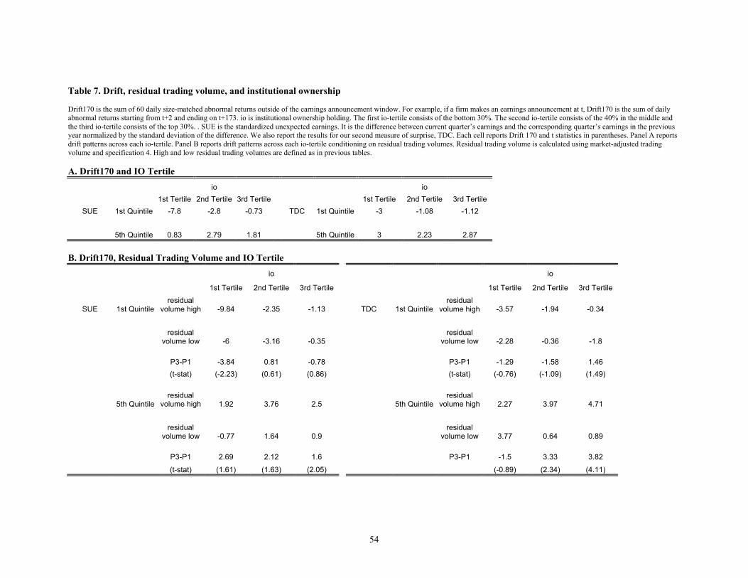
Table 7. Drift, residual trading volume, and institutional ownership Drift170 is the sum of 60 daily size-matched abnormal returns outside of the earnings announcement window. For example, if a firm makes an earnings announcement at t, Drift170 is the sum of daily abnormal returns starting from t+2 and ending on t+173. io is institutional ownership holding. The first io-tertile consists of the bottom 30%. The second io-tertile consists of the 40% in the middle and the third io-tertile consists of the top 30%. . SUE is the standardized unexpected earnings. It is the difference between current quarter’s earnings and the corresponding quarter’s earnings in the previous year normalized by the standard deviation of the difference. We also report the results for our second measure of surprise, TDC. Each cell reports Drift 170 and t statistics in parentheses. Panel A reports drift patterns across each io-tertile. Panel B reports drift patterns across each io-tertile conditioning on residual trading volumes. Residual trading volume is calculated using market-adjusted trading volume and specification 4. High and low residual trading volumes are defined as in previous tables. A. Drift170 and IO Tertile io io

1st Tertile 2nd Tertile 3rd Tertile 1st Tertile 2nd Tertile 3rd Tertile SUE 1st Quintile

-7.8 -2.8 -0.73 TDC

1st Quintile -3 -1.08 -1.12

5th Quintile 0.83 2.79 1.81 5th Quintile 3 2.23 2.87

B. Drift170, Residual Trading Volume and IO Tertile

io io

1st Tertile 2nd Tertile 3rd Tertile 1st Tertile 2nd Tertile 3rd Tertile

SUE

1st Quintile

residual volume high -9.84 -2.35 -1.13 TDC

1st Quintile

residual volume high

-3.57 -1.94 -0.34

residual volume low -6 -3.16 -0.35

residual volume low -2.28 -0.36 -1.8

P3-P1 -3.84 0.81 -0.78 P3-P1 -1.29 -1.58 1.46 (t-stat) (-2.23) (0.61) (0.86) (t-stat) (-0.76) (-1.09) (1.49)

5th Quintile residual

volume high 1.92 3.76 2.5 5th Quintile residual

volume high

2.27 3.97 4.71

residual volume low -0.77 1.64 0.9

residual volume low 3.77 0.64 0.89

P3-P1 2.69 2.12 1.6 P3-P1 -1.5 3.33 3.82

(t-stat) (1.61) (1.63) (2.05) (-0.89) (2.34) (4.11)

54

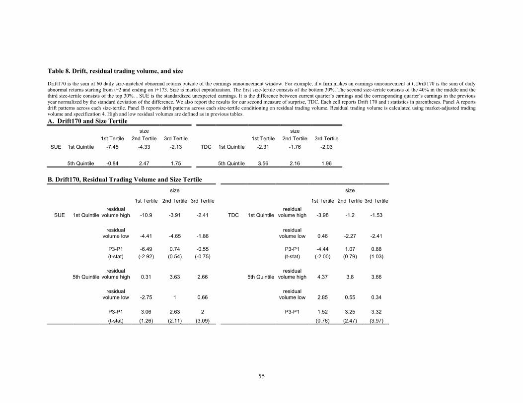
Table 8. Drift, residual trading volume, and size Drift170 is the sum of 60 daily size-matched abnormal returns outside of the earnings announcement window. For example, if a firm makes an earnings announcement at t, Drift170 is the sum of daily abnormal returns starting from t+2 and ending on t+173. Size is market capitalization. The first size-tertile consists of the bottom 30%. The second size-tertile consists of the 40% in the middle and the third size-tertile consists of the top 30%. . SUE is the standardized unexpected earnings. It is the difference between current quarter’s earnings and the corresponding quarter’s earnings in the previous year normalized by the standard deviation of the difference. We also report the results for our second measure of surprise, TDC. Each cell reports Drift 170 and t statistics in parentheses. Panel A reports drift patterns across each size-tertile. Panel B reports drift patterns across each size-tertile conditioning on residual trading volume. Residual trading volume is calculated using market-adjusted trading volume and specification 4. High and low residual volumes are defined as in previous tables. A. Drift170 and Size Tertile size size 1st Tertile 2nd Tertile 3rd Tertile

1st Tertile 2nd Tertile 3rd Tertile SUE 1st Quintile -7.45 -4.33 -2.13 TDC

1st Quintile -2.31 -1.76 -2.03

5th Quintile -0.84 2.47 1.75 5th Quintile 3.56 2.16 1.96

B. Drift170, Residual Trading Volume and Size Tertile

size size

1st Tertile 2nd Tertile 3rd Tertile 1st Tertile 2nd Tertile 3rd Tertile

SUE

1st Quintile


-10.9 -3.91 -2.41 TDC

1st Quintile


-3.98 -1.2 -1.53

residual volume low

-4.41 -4.65 -1.86

residual volume low

0.46 -2.27 -2.41

P3-P1 -6.49 0.74 -0.55 P3-P1 -4.44 1.07 0.88 (t-stat) (-2.92) (0.54) (-0.75) (t-stat) (-2.00) (0.79) (1.03)

5th Quintile residual

volume high

0.31 3.63 2.66 5th Quintile


4.37 3.8 3.66

residual

volume low

-2.75 1 0.66 residual

volume low

2.85 0.55 0.34

P3-P1 3.06 2.63 2 P3-P1 1.52 3.25 3.32

(t-stat) (1.26) (2.11) (3.09) (0.76) (2.47) (3.97)

55

Endnotes 1 In fact, the models by Daniel, Hirshleifer, and Subrahmanyam (1998) and Hong and Stein (1999) try to

explain both underreaction and overreaction of investors in a way consistent with empirically observed

price patterns. Jegadeesh and Titman (1993) report evidence on momentum, i.e., price continuation in the

short to medium term. DeBondt and Thaler (1985) report return reversal at longer horizons. Our paper is

about earnings momentum, thus we focus on the underreaction part of each model.

2 There are several papers that test the implications of the BSV model and report evidence that supports the

model’s predictions (Kim and Rozhkov (1999), Wang (1999), Hvidkjaer (2000)).

3 Thus, investors react to public news in a biased way (self-attribution bias) that will eventually generate

overreaction.

4 The clarity of information represents the degree to which investors agree on its content. Thus clear (or

strong, salient) news will make the distinction between fully rational and underreacting investors less

relevant since all the investors would behave as if they were fully rational investors. We use clarity and

saliency of news interchangeably.

5 When this paper was well under way, we became aware of a paper on a similar topic by Garfinkel and

Sokobin (2000). They argue that large trading volume around an earnings announcement is caused by

existence of diverse private opinions on public information, and drift could be observed as these private

opinions become incorporated into prices. Thus, they argue that larger trading volume precedes larger drift.

But, without the existence of underreacting investors, private opinions that do not become incorporated into

the price on the announcement day should be orthogonal to the content of the public news. In this case, the

direction of the drift caused by private opinions need not be in the same direction as the initial price

reaction to the publicly observable part of the news.

56

6Bernard (1993) looks at the post-earnings announcement drift between 1974 and 1986. We also test

whether our results are robust in earlier time periods. The results are not very different from the ones

reported in this paper.

7 The model in this paper closely follows the structure of Kandel and Pearson (1995).

8 Our model does not consider trading costs explicitly. In the empirical part of the paper, we explicitly

control for the differences in trading costs, since trading costs might affect the trading volume and the

pattern of drift.

9 We have also tried IBES analysts’ mean forecast as the proxy for the expectation measure. The results are

not affected by this change in the expectation measure.

10 We form ten portfolios based on the year-end market capitalization. A size-matched abnormal return is

the difference between an individual firm’s return and a corresponding size decile portfolio’s return.

11 As is apparent from Panels A and B of Figure 1, a drift pattern is clearer when we use SUE as a surprise

measure. The reason could be explained by endogeneity problems inherent in the TDC measure. While the

SUE measure is exogenous to return changes, a TDC measure incorporates investors' reactions after the

news is announced. Thus a low value of TDC could be due to little surprise after the news or could be due

to extreme underreaction from investors.

12 We windsorized our data at 1% and 99% of the distributions of the 60-day drift and market-adjusted

volume to remove the effect of outliers. This does not make much difference in our results.

13 We also run the market model over the 100 days prior to the announcement to calculate the market-

adjusted volume. The results are robust to this specification change.

57

14 In the empirical specification, one might be concerned about the possible negative correlation between

the price change and residual trading volume. Even though this is a theoretical possibility, in our empirical

scheme, it does not pose any significant threat to the unbiasedness of coefficient estimates since we are

estimating cross-sectional regressions. Later in this section, we will check whether there is a systematic

relationship between residual trading volume and absolute price changes. In fact, it turns out that residual

trading volume obtained in cross-sectional regressions does not have a systematic relationship with price

changes.

15 We use heteroskedasticity-robust t-statistics.

16 Results are similar when we use 170-day drift measure.

58

underreaction, trading volume, and post-earnings announcement

Documents