manufacturing execution systems for integration and

Manufacturing Execution Systems for Integration and Intelligence: Guidelines and details for executing the intelligent MES algorithms

(TR-CIM-04.03)

IA LAB

Centre for Intelligent Machines

McGill University

May 20, 2004

Basil Hadjimichael 110248010

TABLE OF CONTENTS 1 Introduction................................................................................................................. 1 2 Genetic Algorithm Hierarchy ..................................................................................... 1 3 Variables for GA......................................................................................................... 2

3.1 Heat Capacity Limit ............................................................................................ 2 3.2 Power Level Fluctuations ................................................................................... 2

4 Running the GA .......................................................................................................... 3 5 GA Performance ......................................................................................................... 5 6 GA Performance with Elitism..................................................................................... 8 7 Modified Makespan .................................................................................................... 9 8 Decision Tree Results ............................................................................................... 10 9 STATEFLOW Model ............................................................................................... 15

9.1 Running the Model ........................................................................................... 15 9.2 Interfacing with STATEFLOW ........................................................................ 16

Industrial Automation Lab

ii

1 Introduction This report will take a new user not familiar with operating in Matlab, through the steps needed to run the algorithms and models presented in “Manufacturing Execution Systems for Integration and Intelligence”. All the files are included in the Appendix for convenience and any references to directories are arranged as found in the accompanying CD disc.

2 Genetic Algorithm Hierarchy The top function for running the Genetic Algorithm (GA) is “genetic_algo.m”. The hierarchy tree of subfunctions called by the GA is as follows:

genetic_algo.m

pop=createPopulation.m

while(generations <= max_gen) for pop

cost.m decode_time.m makespan.m fx_n_fit=generate_f_fit.m end

=ROULETTE WHEEL SELECTION=

cummulate_prob.m gen_mating_pool.m ==CROSSOVER AND MUTATION== new_pop=gen_new_pop.m =============================pop=new_pop generations=generations+1 end

Heats_by_two.m

avg=mean(fx_n_fit) expected_count=fx_n_fit/avg; select_prob=expected_count/pop_size;

A description of each algorithm can be found in the header of the code for the function, see Appendix. Note there are other functions that are called within some of the functions mentioned above, these are not shown here. For more detail into these, the reader is encouraged to use the above hierarchy as a guide and follow the code in its entirety for


1

each algorithm found in the Appendix. The following section explains what some of the variables are used for in the GA.

3 Variables for GA There are many variables to be explained in order to understanding the GA methodology in solving the scheduling problem.

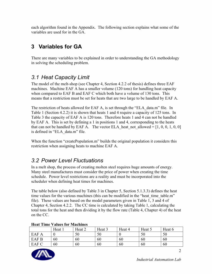
3.1 Heat Capacity Limit The model of the melt-shop (see Chapter 4, Section 4.2.2 of thesis) defines three EAF machines. Machine EAF A has a smaller volume (120 tons) for handling heat capacity when compared to EAF B and EAF C which both have a volume of 130 tons. This means that a restriction must be set for heats that are two large to be handled by EAF A. The restriction of heats allowed for EAF A, is set through the “ELA_data.m” file. In Table 1 (Section 4.2.2) it is shown that heats 1 and 4 require a capacity of 125 tons. In Table 3 the capacity of EAF A is 120 tons. Therefore heats 1 and 4 can not be handled by EAF A. This is set by defining a 1 in positions 1 and 4, corresponding to the heats that can not be handled by EAF A. The vector ELA_heat_not_allowed = [1, 0, 0, 1, 0, 0] is defined in “ELA_data.m” file. When the function “createPopulation.m” builds the original population it considers this restriction when assigning heats to machine EAF A.

3.2 Power Level Fluctuations In a melt shop, the process of creating molten steel requires huge amounts of energy. Many steel manufactures must consider the price of power when creating the time schedule. Power level restrictions are a reality and must be incorporated into the scheduler when defining heat times for machines. The table below (also defined by Table 3 in Chapter 5, Section 5.1.3.3) defines the heat time values for the various machines (this can be modified in the “heat_time_table.m” file). These values are based on the model parameters given in Table 1, 3 and 4 of Chapter 4, Section 4.2.2. The CC time is calculated by taking Table 1, calculating the total tons for the heat and then dividing it by the flow rate (Table 4, Chapter 4) of the heat on the CC. Heat Time Values for Machines Heat 1 Heat 2 Heat 3 Heat 4 Heat 5 Heat 6 EAF A 0 50 50 0 50 50 EAF B 60 60 60 60 60 60 EAF C 60 60 60 60 60 60


2

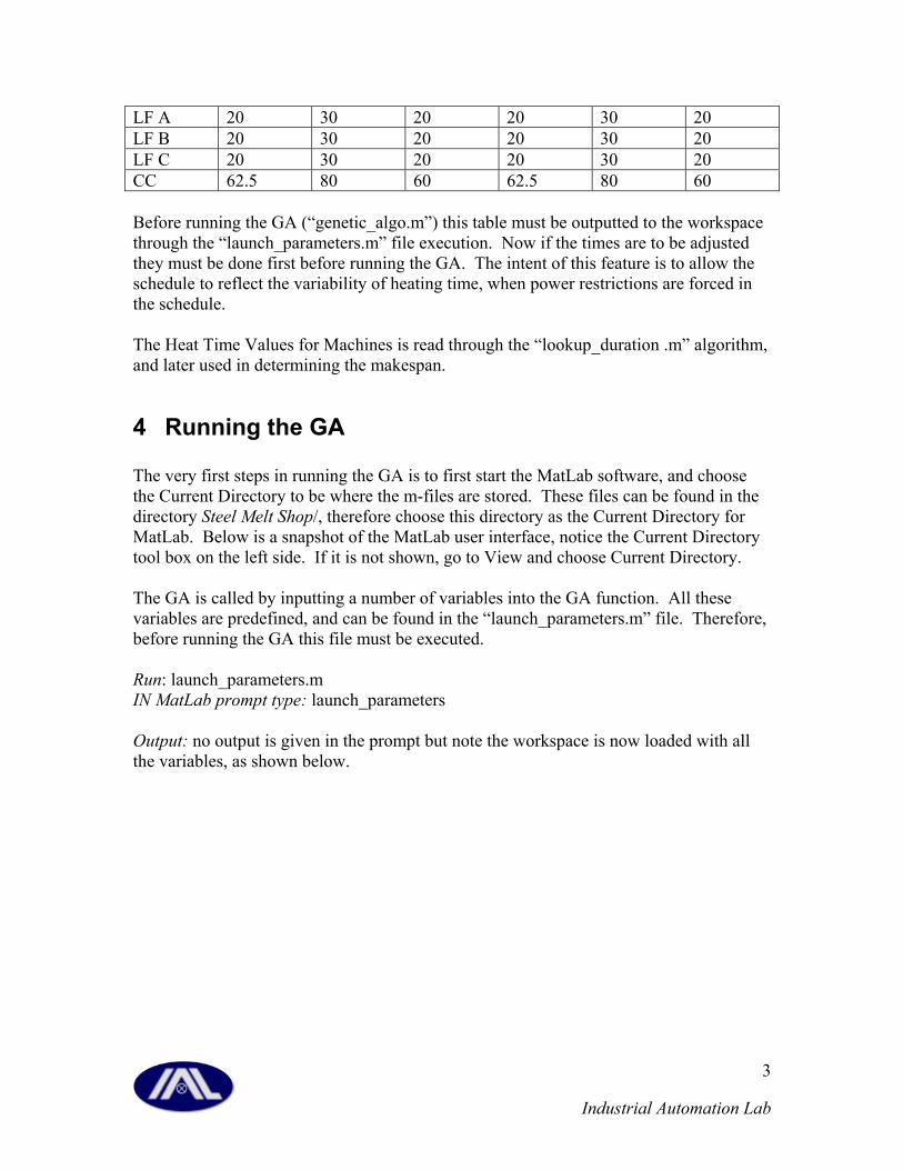
LF A 20 30 20 20 30 20 LF B 20 30 20 20 30 20 LF C 20 30 20 20 30 20 CC 62.5 80 60 62.5 80 60 Before running the GA (“genetic_algo.m”) this table must be outputted to the workspace through the “launch_parameters.m” file execution. Now if the times are to be adjusted they must be done first before running the GA. The intent of this feature is to allow the schedule to reflect the variability of heating time, when power restrictions are forced in the schedule. The Heat Time Values for Machines is read through the “lookup_duration .m” algorithm, and later used in determining the makespan.

4 Running the GA The very first steps in running the GA is to first start the MatLab software, and choose the Current Directory to be where the m-files are stored. These files can be found in the directory Steel Melt Shop/, therefore choose this directory as the Current Directory for MatLab. Below is a snapshot of the MatLab user interface, notice the Current Directory tool box on the left side. If it is not shown, go to View and choose Current Directory. The GA is called by inputting a number of variables into the GA function. All these variables are predefined, and can be found in the “launch_parameters.m” file. Therefore, before running the GA this file must be executed. Run: launch_parameters.m IN MatLab prompt type: launch_parameters Output: no output is given in the prompt but note the workspace is now loaded with all the variables, as shown below.


3

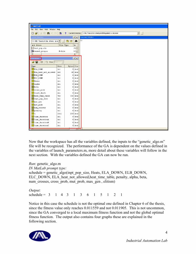
Now that the workspace has all the variables defined, the inputs to the “genetic_algo.m” file will be recognized. The performance of the GA is dependent on the values defined in the variables of launch_parameters.m, more detail about these variables will follow in the next section. With the variables defined the GA can now be run. Run: genetic_algo.m IN MatLab prompt type: schedule = genetic_algo(inpt_pop_size, Heats, ELA_DOWN, ELB_DOWN, ELC_DOWN, ELA_heat_not_allowed,heat_time_table, penalty, alpha, beta, num_crosses, cross_prob, mut_prob, max_gen , elitism) Output: schedule = 3 1 4 3 1 3 6 1 5 1 2 1 Notice in this case the schedule is not the optimal one defined in Chapter 6 of the thesis, since the fitness value only reaches 0.011559 and not 0.011905. This is not uncommon, since the GA converged to a local maximum fitness function and not the global optimal fitness function. The output also contains four graphs these are explained in the following section.


4

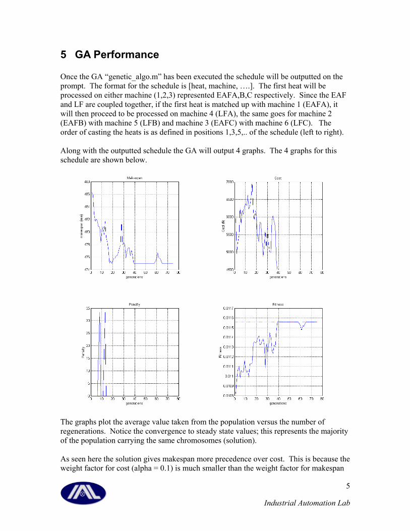
5 GA Performance Once the GA “genetic_algo.m” has been executed the schedule will be outputted on the prompt. The format for the schedule is [heat, machine, ….]. The first heat will be processed on either machine (1,2,3) represented EAFA,B,C respectively. Since the EAF and LF are coupled together, if the first heat is matched up with machine 1 (EAFA), it will then proceed to be processed on machine 4 (LFA), the same goes for machine 2 (EAFB) with machine 5 (LFB) and machine 3 (EAFC) with machine 6 (LFC). The order of casting the heats is as defined in positions 1,3,5,.. of the schedule (left to right). Along with the outputted schedule the GA will output 4 graphs. The 4 graphs for this schedule are shown below.

The graphs plot the average value taken from the population versus the number of regenerations. Notice the convergence to steady state values; this represents the majority of the population carrying the same chromosomes (solution). As seen here the solution gives makespan more precedence over cost. This is because the weight factor for cost (alpha = 0.1) is much smaller than the weight factor for makespan


5

(beta = 40). Both these values can be adjusted in the “launch_parameters.m” file. There is no analysis on the exact relationship between alpha and beta, these values were chosen because the solution does as is desired, to give more importance to makespan over cost. Section 5.1.3.3 of Chapter 5 gets into the detail of how the fitness function was derived. There are two files generated after running the GA. These are the first_pop and last_pop text files. These files can be imported into an excel worksheet for further calculations. The procedure for importing them into an excel worksheet are as follows:

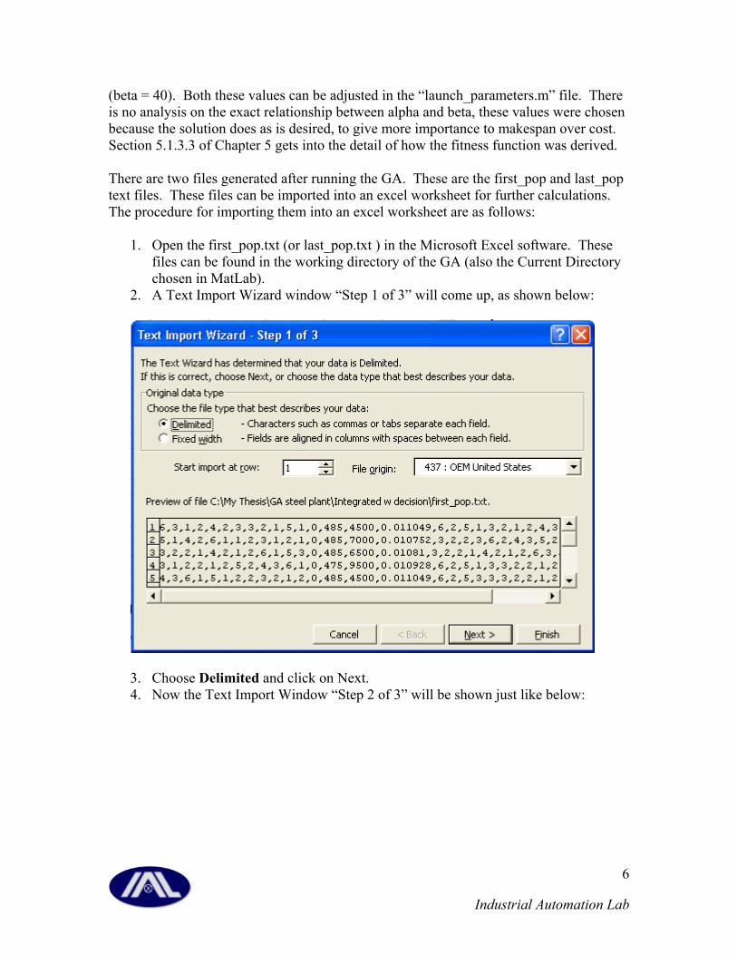
1. Open the first_pop.txt (or last_pop.txt ) in the Microsoft Excel software. These files can be found in the working directory of the GA (also the Current Directory chosen in MatLab).

2. A Text Import Wizard window “Step 1 of 3” will come up, as shown below:

3. Choose Delimited and click on Next. 4. Now the Text Import Window “Step 2 of 3” will be shown just like below:


6

5. Choose Comma and click on Next. 6. In the Text Import Wizard “Step 3 of 3” choose Finish.

If these steps are performed properly the Excel worksheet will have all the data arranged properly in each columns cell. With six heats used (Heats = 6) in “launch_parameters.m” file, the first 12 columns (A-L) will represent the schedule, the number of rows depicts the size of the population, 24 rows means (inpt_pop_size = 24) in the “launch_parameters.m” file. The next four columns M,N,O,P are the penalty, cost, makespan and fitness function respectively for the initial population or final population, depending on whether first_pop.txt or last_pop.txt were opened. The remaining columns represent the schedule defined in the first columns (A-L) with one more generation performed. Other parameters that affect the GA’s performance are: penalty = penalty factor introduced into objective function. See Section 5.1.3.3 of Chapter 5 for a description. DEFAULT: penalty = 400 cross_prob = probability assigned to performing crossover. DEFAULT:cross_prob = 0.8. num_crosses = the number of crossovers to perform when crossover is chosen. For more detail about the crossover algorithm see Section 5.1.5.1 of Chapter 5. DEFAULT: num_crosses = 2.


7

mut_prob = probability of mutation occurring. For more detail about the mutation algorithm see Section 5.1.5.2. DEFAULT mut_prob = 0.01. max_gen = maximum number of generations the genetic algorithm will be run for. DEFAULT: max_gen = 75. Note all of the above DEFAULT values can be changed in “launch_parameters.m” file.

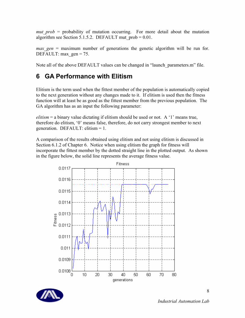
6 GA Performance with Elitism Elitism is the term used when the fittest member of the population is automatically copied to the next generation without any changes made to it. If elitism is used then the fitness function will at least be as good as the fittest member from the previous population. The GA algorithm has as an input the following parameter: elitism = a binary value dictating if elitism should be used or not. A ‘1’ means true, therefore do elitism, ‘0’ means false, therefore, do not carry strongest member to next generation. DEFAULT: elitism = 1. A comparison of the results obtained using elitism and not using elitism is discussed in Section 6.1.2 of Chapter 6. Notice when using elitism the graph for fitness will incorporate the fittest member by the dotted straight line in the plotted output. As shown in the figure below, the solid line represents the average fitness value.


8

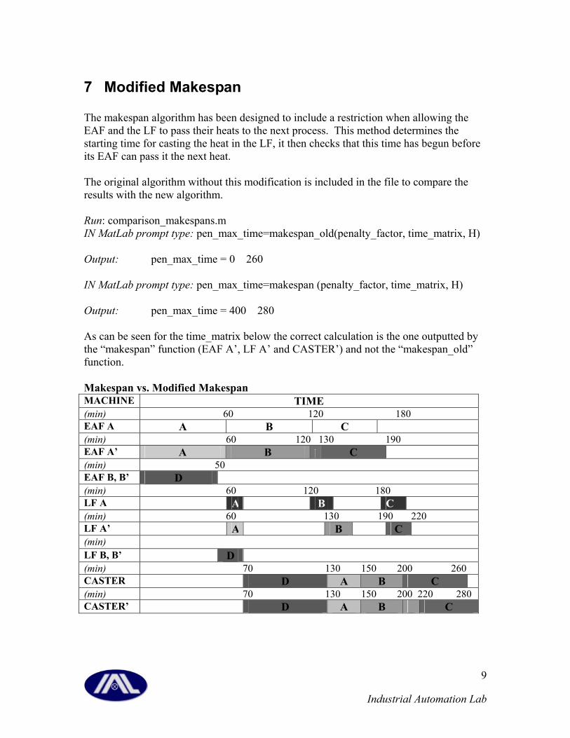
7 Modified Makespan The makespan algorithm has been designed to include a restriction when allowing the EAF and the LF to pass their heats to the next process. This method determines the starting time for casting the heat in the LF, it then checks that this time has begun before its EAF can pass it the next heat. The original algorithm without this modification is included in the file to compare the results with the new algorithm. Run: comparison_makespans.m IN MatLab prompt type: pen_max_time=makespan_old(penalty_factor, time_matrix, H) Output: pen_max_time = 0 260 IN MatLab prompt type: pen_max_time=makespan (penalty_factor, time_matrix, H) Output: pen_max_time = 400 280 As can be seen for the time_matrix below the correct calculation is the one outputted by the “makespan” function (EAF A’, LF A’ and CASTER’) and not the “makespan_old” function. Makespan vs. Modified Makespan MACHINE TIME (min) 60 120 180 EAF A A B C (min) 60 120 130 190 EAF A’ A B C (min) 50 EAF B, B’ D (min) 60 120 180 LF A A B C (min) 60 130 190 220 LF A’ A B C (min) LF B, B’ D (min) 70 130 150 200 260 CASTER D A B C (min) 70 130 150 200 220 280 CASTER’ D A B C


9

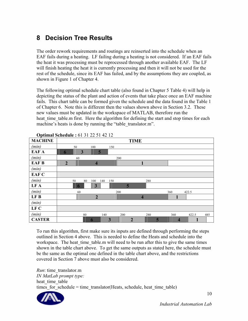
8 Decision Tree Results The order rework requirements and routings are reinserted into the schedule when an EAF fails during a heating. LF failing during a heating is not considered. If an EAF fails the heat it was processing must be reprocessed through another available EAF. The LF will finish heating the heat it is currently processing and then it will not be used for the rest of the schedule, since its EAF has failed, and by the assumptions they are coupled, as shown in Figure 1 of Chapter 4. The following optimal schedule chart table (also found in Chapter 5 Table 4) will help in depicting the status of the plant and action of events that take place once an EAF machine fails. This chart table can be formed given the schedule and the data found in the Table 1 of Chapter 6. Note this is different then the values shown above in Section 3.2. These new values must be updated in the workspace of MATLAB, therefore run the heat_time_table.m first. Here the algorithm for defining the start and stop times for each machine’s heats is done by running the “table_translator.m”. Optimal Schedule : 61 31 22 51 42 12

MACHINE TIME (min) 50 100 150 EAF A 6 3 5 (min) 60 200 EAF B 2 4 1 (min) EAF C (min) 50 80 100 140 150 280 LF A 6 3 5 (min) 60 200 360 422.5 LF B 2 4 1 (min) LF C (min) 80 140 200 280 360 422.5 485 CASTER 6 3 2 5 4 1

To run this algorithm, first make sure its inputs are defined through performing the steps outlined in Section 4 above. This is needed to define the Heats and schedule into the workspace. The heat_time_table.m will need to be run after this to give the same times shown in the table chart above. To get the same outputs as stated here, the schedule must be the same as the optimal one defined in the table chart above, and the restrictions covered in Section 7 above must also be considered. Run: time_translator.m IN MatLab prompt type: heat_time_table times_for_schedule = time_translator(Heats, schedule, heat_time_table)


10

Output: times_for_schedule = 0 0 0 0 50 100 0 0 100 150 0 50 200 360 0 60 0 0 60 200 0 0 0 0 0 0 0 0 0 0 0 0 0 0 0 0 0 0 0 0 100 140 0 0 150 280 50 80 360 422.5 60 200 0 0 200 360 0 0 0 0 0 0 0 0 0 0 0 0 0 0 0 0 422.5 485 200 280 140 200 360 422.5 280 360 80 140 Notice the above table has 12 columns, since there are 6 heats defined and each heat has a start time and end time. The first 2 columns (start and stop time) belong to Heat 1, similarly the last two columns belong to Heat 6. Each row represents a machine. Row 1-3 belong to EAFA-C, while row 3-6 are for LFA-C, and row 7 gives the continuous caster heat times. For an instantaneous failure time of 110 minutes the following data can be extracted from the table above. Note this data is formulated by the algorithm “decode_decision_parameters.m” and it must be run before running the decision tree algorithm (decision_tree.m). To understand what the “decode_decision_parameters.m” algorithm does, let us take note of all the data that must be extracted from the table above at the time of failure in order to be used by the decision making algorithm. For the LF’s it can be seen that the active heats are 3 for LFA and 2 for LFB, as defined in “LF_machine = [3,2,0]”. Each has a time left of 30 minutes and 90 minutes respectively. These are defined in “time_left_in_LF”. For the EAF’s, there are two active heats, however one of them heat 4 can not be completed since EAFB has failed. Hence only one heat is active since the failed one must be reprocessed again at a later time. This leads to defining a zero for EAFB, and the rest as; “EAF_machine = [5, 0, 0]” with times defined as “time_left_in_EAF = [40, 0, 0]”. The continuous caster has heat 6 active at time of failure (“heat_in_CC = 6”) and the time left is 30 minutes (“time_left_in_CC = 30”). Lastly, the heats not yet active at time of failure is 1, with a scheduled process on EAF B (machine 2), hence heats_left_in_schedule = [1, 2]. Notice the failed heat 4 on EAF B is also included since it must be redone. With the above data defined in the file “decode_decision_parameters.m” (also given below in the APPENDIX for convenience), running it will produce this data: Run: decode_decision_parameters.m IN MatLab prompt type: instant_ftime = 110; EAF_failed = 2;


11

[LF_machine, EAF_machine, time_left_in_LF, time_left_in_EAF, heat_in_CC, time_left_in_CC, heats_left_in_schedule] = decode_decision_parameters(times_for_schedule, instant_ftime, EAF_failed, Heats, schedule) Output: LF_machine = 3 2 0 EAF_machine = 5 0 0 time_left_in_LF = 30 90 0 time_left_in_EAF = 40 0 0 heat_in_CC = 6 time_left_in_CC = 30 heats_left_in_schedule = 4 2 1 2 Also see workspace, where all the outputted parameters have been defined Now the decision tree algorithm (“decision_tree.m”) can be run. Run: decision_tree.m IN MatLab prompt type: schedule = decision_tree(inpt_pop_size, Heats, EAF_failed, ELA_DOWN, ELB_DOWN, ELC_DOWN, ELA_heat_not_allowed, penalty, alpha, beta, num_crosses, cross_prob, mut_prob, max_gen, heats_left_in_schedule, EAF_machine, time_left_in_EAF, LF_machine, time_left_in_LF, heat_in_CC, time_left_in_CC, heat_time_table) Output: schedule = 3 4 2 5 5 1 1 3 4 3 The following charts are also outputted:


12

The above schedule is interpreted by first noting if a zero exists as a first element. This means Turnaround can not be avoided with this failure. This is not the case here, since a zero is not present in the first element. The active LF heats are dealt with by casting them in the order given in the schedule. First cast heat 3 in LF A (machine 4), then cast heat 2 from LF B (machine 5). The next active heats are found in the EAFs. In this case only heat 5 in EAF A (machine 1) was active at time of failure and should be cast next following heat 2. After this the inactive heats are processed heat 1 then heat 4 in EAFC (machine 3), this is coupled to LFC (machine 6). For a description of the decision tree algorithm see Chapter 5 Sections 5.4.3 to 5.4.5. The four charts above are the performance of the modified GA, for solving the schedule starting with the first heat fixed, and followed by the inactive heats. The first heat fixed is taken as the last cast from the active heats [order(active_size-1)], for this case it will be heat 5 processed through EAF A [order(active_size)] and LFA. The modifications to the GA are as follows: Modified GA: sub_genetic_algo.m Inputs as described above: first_heat = order(active_size-1); first_machine = order(active_size);


13

These inputs along with the inactive heats left [heats_left], are inputted into the GA, along with the failed EAF (EAF_DOWN) to be used firstly in the function “createSUBPopulation.m”. This function creates the original population by arranging the heats_left in all possible combinations, and fixing the first heat and machine to be as defined above. The function then matches up the inactive heats to arbitrary machines A,B,C. It then removes the failed machine with one of the other two, and checks that the machine assigned to the inactive heat can handle the heat’s capacity (see Heat Capacity Limit above). The remaining part of the sub_genetic_algo.m file is similar to the original genetic algorithm “genetic_algo.m”. When performing mutation it still considers the failed machine and the heat’s capacity when mutating the machine.


14

9 STATEFLOW Model Before reading this the reader should refer to Section 4.3 of the thesis for a background on the STATEFLOW model.

9.1 Running the Model There are a few things that need to be familiarized in STATEFLOW/SIMULINK before understanding how to interpret the model simulation. These are the Explorer and Debugger found in STATEFLOW, and the Sources; “from Workspace” blocks found in SIMULINK. The model can be opened by simply clicking on “system_model.mdl” found in the “Steel Melt-Shop” directory of the accompanying disk. Upon clicking on “system_model.mdl” a new SIMULINK window will open, with the top level system model shown. The five main blocks can be clicked on to enter into the STATEFLOW modules. Clicking on any of these five blocks will open a new STATEFLOW chart window for the appropriate block chosen. By choosing Tools/Explorer in the STATEFLOW (chart) window, a new Exploring window will open. This window defines all the data signals that are used for this block in SIMULINK. Notice the input, output and Local signals and the ranges for each value defined. For input and output signals the reference is with respect to the SIMULINK frame model. For example, for the EAF_LF_A block the input “eaf_capactiy” is inputted through the SIMULINK model into the STATEFLOW block EAF_LF_A. Notice in SIMULINK this value is defined as 120, as is displayed in the Explorer window for this block. With this understanding of the SIMULINK and STATEFLOW entities, it must be noted that running the model can only be done after the workspace in MATLAB is loaded with the proper parameters. This is where the interfacing for MATLAB and the SIMULINK/STATEFLOW come together. Before going into these details, the user should understand the “from Workspace” block. In the model there are four of these blocks defined, they are:

1. sf_schedule 2. ELA_status 3. ELB_status 4. ELC_status

Each of these variables must be defined in the MatLab Workspace to be recognized in the model. See “Interfacing with Stateflow” Section 9.2 below for detail on sending these variables to the Workspace before reading on.


15

Running the model can be done in two ways. Through the SIMULINK window click on ‘Simulation’ then choose ‘Start’, or through any of the STATEFLOW windows choose ‘Simulation’ then choose ‘Start’. Now click the “Start” switch to 1 in the SIMULINK model. The model can also be run in Debug mode; this means the user clicks each time the next event should be triggered. This is done in any of the STATEFLOW windows by choosing ‘Tools’ and then picking ‘Debug’. Now click the Start button in the Debug mode followed by the Continue button each time you want another event to occur. At about the 3rd event (i.e. 3 clicks), go the SIMULINK model and click the “Start” switch to 1. Notice once everything has been initialized the model will run and the outputs will be sent to the Command Prompt in MatLab. These outputs represent the action events in the order they occur in the model.

9.2 Interfacing with STATEFLOW The steps to follow here must be done after the user has run the GA and has outputted a schedule to the workspace (Section 4: RUNNING THE GA). Assuming the GA executed a schedule to the workspace in the format [heat, machine, …]. The next step to perform will reformat the schedule in order for the Simulink Model to recognize the “Input from Workspace” sf_schedule block. This reformatting is done by running the algorithm “ga2sf.m”: Run: ga2sf.m IN MatLab prompt type: ga_schedule = schedule sf_schedule = ga2sf(first_shift, ga_schedule, Heats) Output: sf_schedule = 0 3 2 6 2 5 1 30 3 2 6 2 5 1 60 3 2 6 2 5 1 90 3 2 6 2 5 1 120 3 2 6 2 5 1 150 3 2 6 2 5 1 180 3 2 6 2 5 1 210 3 2 6 2 5 1 240 3 2 6 2 5 1 This is the schedule outputted by the GA for the first three heats (first_shift = 1). If first_shift = 0, then the “ga2sf.m” algorithm will outputted the second shift. sf_schedule =


16

0 2 2 4 3 1 3 30 2 2 4 3 1 3 60 2 2 4 3 1 3 90 2 2 4 3 1 3 120 2 2 4 3 1 3 150 2 2 4 3 1 3 180 2 2 4 3 1 3 210 2 2 4 3 1 3 240 2 2 4 3 1 3 These are based on ga_schedule = 3 2 6 2 5 1 2 2 4 3 1 3. With the “Input from Workspace” sf_schedule block defined, the EAF_LF input blocks must now be defined. This is done by running the three algorithms one for each EAF_LF block. When running make sure that sf_schedule is the one taken with first_shift = 1, in order to obtain the output shown below. Run: ELAstatus.m IN MatLab prompt type: ELA_status = ELAstatus(sf_schedule, heat_time_table) Output: ELA_status = 0 50 30 10 50 30 20 50 30 30 50 30 40 50 30 50 50 30 60 50 30 70 50 30 80 50 30 90 50 30 100 50 30 110 50 30 120 50 30 130 50 30 140 50 30 150 50 30 160 50 30 170 50 30 180 50 30 190 50 30 200 50 30


17

210 50 30 220 50 30 230 50 30 240 50 30 This array is now loaded into the workspace and when running the model the “Input from Workspace” ELA_status block will read this array in order to determine the heating time needed during the simulation for the first half of the day. Notice since there is only one heat processed by EAF_LF_A in the first half of the day the second column for EAF heating time and third column for LF heating time do not change. This is not the case for EAF_LF_B. A similar approach can be done for ELB_status and ELC_status blocks. For ELB_status: Run: ELBstatus.m IN MatLab prompt type: ELB_status = ELBstatus(sf_schedule, heat_time_table) Output: ELB_status = 0 60 20 10 60 20 20 60 20 30 60 20 40 60 20 50 60 20 60 60 20 70 60 20 80 60 20 90 60 20 100 60 20 110 60 20 120 60 20 130 60 20 140 60 20 150 60 20 160 60 20 170 60 20 180 60 20 190 60 20 200 60 20 210 60 20 220 60 20 230 60 20


18

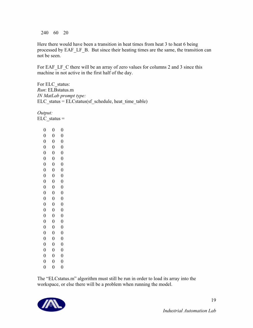
240 60 20 Here there would have been a transition in heat times from heat 3 to heat 6 being processed by EAF_LF_B. But since their heating times are the same, the transition can not be seen. For EAF_LF_C there will be an array of zero values for columns 2 and 3 since this machine in not active in the first half of the day. For ELC_status: Run: ELBstatus.m IN MatLab prompt type: ELC_status = ELCstatus(sf_schedule, heat_time_table) Output: ELC_status = 0 0 0 0 0 0 0 0 0 0 0 0 0 0 0 0 0 0 0 0 0 0 0 0 0 0 0 0 0 0 0 0 0 0 0 0 0 0 0 0 0 0 0 0 0 0 0 0 0 0 0 0 0 0 0 0 0 0 0 0 0 0 0 0 0 0 0 0 0 0 0 0 0 0 0 The “ELCstatus.m” algorithm must still be run in order to load its array into the workspace, or else there will be a problem when running the model.


19

Important Note: The plant model was built with a capacity to handle 3 heats in one shift (half-day). This means the Simulink Model can only simulate 3 heats consecutively. The next heats in the schedule following the first three must be loaded into the model by redefining sf_schedule (with first_shift = 0). Followed by rerunning ELA_status, ELB_status and ELC_status again with the new sf_shedule for the second half of the day defined.


20

APPENDIX comparison_makespans %makespan_old_vs_new %------------------------------ %run this file to define these parameters into the MATLAB workspace %------------------------------ penalty_factor=400; %time_matrix arranges heats, in schedule format first row is first heat to be cast and last row is last heat to be cast %format: 6 columns and 4 rows for 4 heats. %Columns 1,3,5 represent the machines the heat will visit EAFA=1,LFA=4,CC=7 %Collumns 2,4,6 are the times to process the heat on each machine respectively time_matrix=[2, 50, 5, 20, 7, 60; 1, 60, 4, 20, 7, 20; 1, 60, 4, 15, 7, 50; 1, 60, 4, 20, 7, 60]; H=4; cost function y = cost(entry,H) %------------------------------ % Estimate the cost for transition from one grade of heat to another % Input ENTRY is 1*6 matrix. % Output y is a scaler for the cost in unit of $. % Here we assume one and only one billet created during transition. % One billet of GA is 25 tons, one billet of GB or GC is 20 tons. % From\To GA GB GC GD GE GF % GA 0 $200/ton $100/ton 0 $200/ton $100/ton % GB 0 0 0 0 0 0 % GC 0 $100/ton 0 0 $100/ton 0 % GD 0 $200/ton $100/ton 0 $200/ton $100/ton % GE 0 0 0 0 0 0 % GF 0 $100/ton 0 0 $100/ton 0 % %i.e. % From\To GA GB GC GD GE GF % GA 0 $5,000 $2,500 0 $5,000 $2,500 % GB 0 0 0 0 0 0 % GC 0 $2,000 0 0 $2,000 0 % GD 0 $5,000 $2,500 0 $5,000 $2,500 % GE 0 0 0 0 0 0 % GF 0 $2,000 0 0 $2,000 0 %------------------------------ % first a reference table of 6:6 matrix for cost of upto 6 heats was made assuming ton quantities specified above [m,n] = size(entry); if (n <3) error('Cost cannot be given since there is no transitions of heats'); return; end lookup = [0 5000 2500 0 5000 2500; 0 0 0 0 0 0; 0 2000 0 0 2000 0;


21 0 5000 2500 0 5000 2500; 0 0 0 0 0 0; 0 2000 0 0 2000 0];

y = 0; % initialize cost to zero % check the first transition cost i = entry(1); j = entry(3); y = lookup(i,j) ; % check the second transition cost if (H > 2) i = entry(3); j = entry(5); y = y + lookup(i, j); end % check the third transition cost if (H > 3) i = entry(5); j = entry(7); y = y + lookup(i, j); end % check the fourth transition cost if (H > 4) i = entry(7); j = entry(9); y = y + lookup(i, j); end % check the fifth transition cost if (H > 5) i = entry(9); j = entry(11); y = y + lookup(i, j); end create_machine_table function create_machine_table(H) %------------------------------ %this function will create a lookup table where the rows represent the number of machines (max is 3 machines and therefore 7 rows) %All 7 rows are given since the table defines the times for all the machines. If a machine is down the initial population will %know this and therefore will not be able to choose that machine from the table defined below %col 1 is the machine #, col 2 is grade, col 3 is process duration for the given machine, and given grade %the machine table will initially be all zeros %------------------------------ global machine_table machine_table=zeros(7, H); for j = 1:H for i = 1:7 machine_table(i,j)= heat_time_table(i,j); end end


22

createPopulation function pop = createPopulation(n, H, ELA_DOWN, ELB_DOWN, ELC_DOWN, ELA_heat_not_allowed) %------------------------------ % Create Population for the Genetic Algorithm. % CREATEPOPULATION(N), where N is a scaler, is the number of elements % in the genereated population. % H represents the number of heats (H <= 6)and M the number of Machines (EAF_LF; M <=3). Restriction due to machine_table % Each element is vector with row=1, column = 6, here columns 1, 3 and % 5 are for heat type, have range 1-3; columns 2, 4 and 6 define the % using ELFA or ELFB, have range 1-2 % The output will be a matrox of N *(H*2) %------------------------------ if ((n<0)|(H<0)|(H>6)) error('Range for inpt_pop_size > 0, Heats (0-6)'); return; end pop = zeros(n, (H*2)); % initialize n*6 matrix pop with zeros myperms = perms(1:H); % get permutation of H, here myperms % will be H!*H matrix (represnts initial order of Heats) b = round(3*rand(n,H)); % n*H matrix, with elements range 0 - M (represents initial order of Machines; M <=3) % adjust the make matrix 'b' elements of 0 to 1, while taking into account the machines that are DOWN all_machines_up = 0; %originally assume not all machines are up, unless status says they are for i = 1:n for j = 1:H %note we can generate a schedule if one machine is down out of the three, but not if two are down %Case A (no machines are down) if ((ELA_DOWN == 0) & (ELB_DOWN == 0) & (ELC_DOWN == 0)) all_machines_up = 1; if ( b(i,j) == 0 ) b(i,j) = 1; % ???check if this affects solution ie should it be a 2,3 instead of a end end %Case B (1 machine is down, can't have two machines down, since this is trivial schedule) if ( (ELA_DOWN ==1) & (all_machines_up == 0)) if (b(i,j) == 1) b(i,j) = 2; end if (b(i,j) == 0) b(i,j) = 3; %since ELB and ELC up, give some to ELC since ELB gets all of ELA's heats end end if ( (ELB_DOWN ==1) & (all_machines_up == 0)) if (b(i,j) == 2) b(i,j) = 3; end if (b(i,j) == 0) b(i,j) = 1; end end


23

if ( (ELC_DOWN ==1) & (all_machines_up == 0)) if (b(i,j) == 3) b(i,j) = 1; end if (b(i,j) == 0) b(i,j) = 2; end end end end for i = 1:n for j = 1:H %here, column 2, 4, 6 of pop from column 1, 2, 3 of b pop(i,j*2) = b(i,j); end end % adjust the make matrix 'pop' elements if any heats are to large for the capacity of EAFA for i = 1:n x = ceil(factorial(H)*rand(1)); % get a random value range 1 - H! for j = 1:H pop(i,j*2-1) = myperms(x, j); if ( (pop(i, j*2) == 1) & (ELA_heat_not_allowed(pop(i, j*2-1)) == 1) & (ELB_DOWN == 0) ) % if this heat is not allowed pop(i, j*2) = 2; % we need bind it to ELFB (=2) else if ((pop(i, j*2) == 1) & (ELA_heat_not_allowed(pop(i, j*2-1)) == 1) ) pop(i, j*2) = 3; % we need bind it to ELFC (=3) since ELFB is down end end % end if end end createSUBPopulation function pop = createSUBPopulation(n, first_heat, first_machine, heats_left, ELA_DOWN, ELB_DOWN, ELC_DOWN, ELA_heat_not_allowed) %------------------------------ %this function is part of the decision tree algorithm %it is similar to the createPopulation algorithm, however it considers: % -machine constraints due to failure % -fixing the first heat (last active heat), this is based on the order of the active heats given by the decision tree %------------------------------ [R,C] = size(heats_left); H = C + 1; if ((n<0)|(H<0)|(H>6)) error('Range for inpt_pop_size > 0, Heats (0-6)'); return; end pop = zeros(n, (H)); % initialize matrix pop with zeros, rows is equal to size of pop, and columns equals #of heats left + first_heat myperms = perms(heats_left); %create all possible combinations of heats_left,


24

%Now will add first_heat as first column for everyone for i = 1:factorial(C) myperms_prime(i,:) = cat(2,first_heat, myperms(i,:)); end b = round(3*rand(n,H)); % n*(heats_left+1) matrix, with elements range 0 - M (represents initial order of Machines; M <=3) % adjust the make matrix 'b' elements of 0 to 1, while taking into account the machines that are DOWN %using general code even though know one machine has failed all_machines_up = 0; %originally assume not all machines are up, unless status says they are for i = 1:n for j = 1:H %note we can generate a schedule if one machine is down out of the three, but not if two are down %Case A (no machines are down) if ((ELA_DOWN == 0) & (ELB_DOWN == 0) & (ELC_DOWN == 0)) all_machines_up = 1; if ( b(i,j) == 0 ) b(i,j) = 1; % ???check if this affects solution ie should it be a 2,3 instead of a end end %Case B (1 machine is down, can't have two machines down, since this is trivial schedule) if ( (ELA_DOWN ==1) & (all_machines_up == 0)) if (b(i,j) == 1) b(i,j) = 2; end if (b(i,j) == 0) b(i,j) = 3; %since ELB and ELC up, give some to ELC since ELB gets all of ELA's heats end end if ( (ELB_DOWN ==1) & (all_machines_up == 0)) if (b(i,j) == 2) b(i,j) = 3; end if (b(i,j) == 0) b(i,j) = 1; end end if ( (ELC_DOWN ==1) & (all_machines_up == 0)) if (b(i,j) == 3) b(i,j) = 1; end if (b(i,j) == 0) b(i,j) = 2; end end end end for i = 1:n for j = 1:H %here, column 2, 4, 6 of pop from column 1, 2, 3 of b if (j == 1) pop(i,j*2) = first_machine; %force first heat to first machine


25 else

pop(i,j*2) = b(i,j); end end end % adjust the make matrix 'pop' elements if any heats are to large for the capacity of EAFA for i = 1:n x = ceil(factorial(C)*rand(1)); % get a random value range 1 - C! , recall C = size(heats_left), the first_heat will not give more combinations for j = 1:H pop(i,j*2-1) = myperms_prime(x, j); if ( (pop(i, j*2) == 1) & (ELA_heat_not_allowed(pop(i, j*2-1)) == 1) & (ELB_DOWN == 0) ) % if this heat is not allowed pop(i, j*2) = 2; % we need bind it to ELFB (=2) else if ((pop(i, j*2) == 1) & (ELA_heat_not_allowed(pop(i, j*2-1)) == 1) ) pop(i, j*2) = 3; % we need bind it to ELFC (=3) since ELFB is down end end % end if end end cross_over function off1=cross_over(parent1, parent2, cross_prob, H, num_crosses) %------------------------------------------------- %determine whether you cross over or not based on cross_prob %the algorithm is as follows. %1. randomly choose to positions e.g. 1,2 %2. offspring inherits what is in position 3 of parent 1 %3. offspring inherits the remaining heat and EAF ordering from parent 2 % e.g. P1 is [1 2; 2 2; 3 1] and P2 is [2 1; 3 2; 1 2] %the crossover positions are 1 and 2 %the offspring is [2 1; 1 2; 3 1] %------------------------------------------------- cross_or_not=rand; if cross_or_not < cross_prob 'cross'; %if the random number is not between 1 and H, keep generating until you get one cross_sites=fix((H+1)*rand(1,num_crosses)); %1 row, num_crosses columns, with each column in (0-H) range num_crosses_not_in_range = 0; %assume not correct (i.e. there are two identical values or values not in range) num_crosses_not_identical = 0; while (num_crosses_not_identical < (num_crosses*num_crosses + 1) ) switch num_crosses_not_in_range case(0) if ( ( max(cross_sites) > H) | ( min(cross_sites) < 1) ) cross_sites=fix((H+1)*rand(1,num_crosses)); %not in range therefore regenerate cross_sites else num_crosses_not_identical = 1; num_crosses_not_in_range = 1; end


26

case(1) % check that no two values are identical in cross_sites m1 = 1; %reset m1 and m2 incase got switched to case(0) during case(1) m2 = 1; for m1 = 1:num_crosses for m2 = 1:num_crosses if ( (m1 ~= m2) & (cross_sites(m1) == cross_sites(m2)) ) cross_sites=fix((H+1)*rand(1,num_crosses)); num_crosses_not_in_range = 0; %go back to start and check all conditions again else num_crosses_not_identical = num_crosses_not_identical + 1; % if all ok this value will be num_crosses*num_crosses + 1 end end end otherwise num_crosses_not_correct = 0; end %end switch end %end while %disp(cross_sites); off1=zeros(H,2); for j = 1:H if ( j ~= cross_sites(1:num_crosses) ) off1(j,1)=parent1(j,1); off1(j,2)=parent1(j,2); end end %find the position of jobs in parent2 that correspond to the jobs in the %cross_sites location in parent1 for j=1:num_crosses job=parent1(cross_sites(j),1); %??gives error with index dimensions for k=1:H %find the position of job in parent2 if (parent2(k,1) == job) order(j)=k; %maintains order of parent 2 heat(j,1)=parent2(k,1); heat(j,2)=parent2(k,2); end end end %put heats of parent2 into off1 while keeping order of parent2 the same (order(k) with smallest value goes first) positions = zeros(num_crosses); positions = sort(order); for i = 1:num_crosses; j= 1; %set counter while (j <= H) if (off1(j,1)==0)


27 %find 'zero in off1, place postion(i) of heat there

off1(j,1)=parent2(positions(1,i),1); off1(j,2)=parent2(positions(1,i),2); j = H+1; end j = j + 1; end end else %disp('dont cross'); %output is now just the parents off1=parent1; end cummulate_prob function cum_prob=cummulate_prob(pop_size, select_prob) %--------------------------------------------------- %this function inputs the selection probability of all chromosomes in the %population, and outputs the cummulative probability of all chromosomes %--------------------------------------------------- cum_prob(1,1)=select_prob(1,1); for(i=2:pop_size) cum_prob(i,1)=cum_prob(i-1,1) + select_prob(i,1); end decision_tree function schedule = decision_tree(inpt_pop_size, Heats, EAF_failed, ELA_DOWN, ELB_DOWN, ELC_DOWN, ELA_heat_not_allowed, penalty, alpha, beta, num_crosses, cross_prob, mut_prob, max_gen, heats_left_in_schedule, EAF_machine, time_left_in_EAF, LF_machine, time_left_in_LF, heat_in_CC, time_left_in_CC, heat_time_table) %---------------------------------------------------------- %TREE ALGORTHIM %need table of times for day schedule provided by data that breaks down the schedule into individual start and stop times for each machine's heats %EXAMPLE: for optimal schedule see times_for_schedule.m file %find interval where failure occurred for CC %STAGE ONE IS TO ORDER THE HEATS ACTIVE IN THE SYSTEM INTO THE BEST ORDER POSSIBLE %STAGE 1a. Do LFs %STAGE 1b. Do EAFs %STAGE TWO runs a modified GA %CASES %call GA only if needed. %TEST 1: If heats not done can still be done in order given by schedule, %TEST 2: while still having the FIRST in heats not done following the LAST in active heats as given in schedule. %TEST 1 & 2 must be satisfied to not call the GA.


28

%TEST 1 or 2 failed, so redo GA starting from last heat in order %No order was found, case occurs when no heats are active so call GA redo whole schedule with failed machine taken out %---------------------------------------------------------- %STAGE 1a. order = decision_tree_one(LF_machine, time_left_in_LF, heat_in_CC, time_left_in_CC); %STAGE 1b. [rows,LF_size] = size(order); if (LF_size > 0) %follow based on LF order. Need to shift machine numbers by 3 %careful if turnaround don't want to shift this number by 3, %only want order of machines to be 4,5,6 rather than 1,2,3 %if odd number know a zero was added at beginning for Turnaround TURNAROUND = rem(LF_size, 2); %this will equal 1 if turnaround since order will be an odd #, and 0 if no Turnaround (even #) if (TURNAROUND == 1) for i = 3:2:LF_size order(i) = order(i) + 3; %add +3 to machine numbers, to reflect machines LFA,B,C by 4,5,6 so 1,2,3 will belong to EAFA,B,C end else for i = 2:2:LF_size order(i) = order(i) + 3; end end %get time to cast heats in LFs cc_time_for_LF_heats = 0; %want to know start times for each casting, first one begins after heat_in_CC is finished casting_start_time_for_activeLF = zeros(1,3); current_time_upto_now = time_left_in_CC; %time reference is failure time %Use this later to change time_left_in_CC_prime for i = 1:3 if (LF_machine(i) ~= 0) cc_time_for_LF_heats = cc_time_for_LF_heats + heat_time_table(7, LF_machine(i)); end end %DO time_left_in_CC_prime, need this to heck if heat in EAF can be cast w/o Turnaround occuring %when calling decision_tree_one->time frame for time_left_in_CC must shift to reflect the LFs being cast %must know if Turnaround occurred for LFs since this adds 20 minutes if (order(1) == 0) %Turnaround has occurred % ~ 20min + time of casting LF's + time_left_in_CC > time_left_in_EAF time_left_in_CC_prime = 20 + time_left_in_CC + cc_time_for_LF_heats; current_time_upto_now = current_time_upto_now + 20; else %no Turnaround has occurred


29 % ~ time_left_in_cc + cast times for LF's found in order vector > time_left_in_EAF

time_left_in_CC_prime = time_left_in_CC + cc_time_for_LF_heats; end if (TURNAROUND == 1) for i =3:2:LF_size j = order(i); %get first machine in order, recall above machine LFs renumbered from 1,2,3 to 4,5,6 to reflect LFA,B,C k = order(i-1); %get heat for the machine casting_start_time_for_activeLF(j-3)= current_time_upto_now; %recall casting_start_time_for_activeLF is a vector of size 3, where 1 is for LFA current_time_upto_now = current_time_upto_now + heat_time_table(7, k); end else for i =2:2:LF_size j = order(i); %get first machine in order, recall above machine LFs renumbered from 1,2,3 to 4,5,6 to reflect LFA,B,C k = order(i-1); %get heat for the machine casting_start_time_for_activeLF(j-3)= current_time_upto_now; current_time_upto_now = current_time_upto_now + heat_time_table(7, k); end end %HERE must remember EAF must be followed by LF and therefore check LF free, %if not need to wait for it to be free before sending active EAF heat to LF time_left_in_EAF_prime = zeros(1,3); for i = 1:3 %do for all active EAFs if (EAF_machine(i) ~= 0) %here time_left_in_EAF_prime must reflect its time plus time needed on its LF. %CRITERIA: - EAF and LF must have both been active if (LF_machine(i) ~= 0) %IF first CRITERIA met: find start time of the LF based on order, and check its start time is before time EAF is done if (casting_start_time_for_activeLF(i) > time_left_in_EAF(i)) time_left_in_EAF_prime(i) = casting_start_time_for_activeLF(i)+ heat_time_table(i+3, EAF_machine(i)); else time_left_in_EAF_prime(i) = time_left_in_EAF(i) + heat_time_table(i+3, EAF_machine(i)); end else %here not restricted to waiting for LF so just add time needed on LF for heat in EAF before ready to be cast time_left_in_EAF_prime(i) = time_left_in_EAF(i) + heat_time_table(i+3, EAF_machine(i)); end end end order2 = decision_tree_one(EAF_machine, time_left_in_EAF_prime, order((LF_size)-1), time_left_in_CC_prime); order = cat(2, order, order2); else %still at instantaneous time of failure


30 %no LFs so have to do ordering with only EAFs

order = decision_tree_one(EAF_machine, time_left_in_EAF, heat_in_CC, time_left_in_CC); end %STAGE 2 - GA part [rows,active_size] = size(order); if (active_size ~= 0) %call GA only if needed. TEST 1: If heats not done can still be done in order given by schedule, TEST 2: while still having the FIRST in heats not %done following the LAST in active heats as given in schedule. %TEST 1 & 2 must be satisfied to not call the GA. %TEST 1 -check if failed machine is found in "heats_left_in_schedule" [rows,non_active_size] = size(heats_left_in_schedule); REDO_GA = 0; %check machines assigned for non_active_heats for i = 2:2:non_active_size if (heats_left_in_schedule(i) == EAF_failed) %must redo GA REDO_GA = 1; end end %TEST 2 -get last active_heat cast and first non_active_heat to be cast, and compare to schedule if (REDO_GA == 0) comapre_transition_active_to_notactive = [order(active_size-1), heats_left_in_schedule(1)]; for i = 1:2:Heats*2 if (schedule(i) == order(active_size-1)) compare_to_schedule = [schedule(i), schedule(i+2)]; end end if ( (comapre_transition_active_to_notactive(1) == compare_to_schedule(1)) & (comapre_transition_active_to_notactive(2) == compare_to_schedule(2)) ) %ok to keep schedule schedule = cat(2, order, heats_left_in_schedule); end else %TEST 1 or 2 failed, so redo GA starting from last heat in order, as first in GA and rest of non_active heats, also %remove EAF_failed when solving GA. %initialize ELA_DOWN = 0; ELB_DOWN = 0; ELC_DOWN = 0; if (EAF_failed == 1) ELA_DOWN = 1; elseif (EAF_failed == 2) ELB_DOWN = 1; else ELC_DOWN = 1; end %here-have to adjust subCreate_pop.


31 first_heat = order(active_size-1);

first_machine = order(active_size); %format of heats_left_in_schedule = [heat, machine,..], only want heat. j = 0; for i =1:(non_active_size/2) heats_left(i) = heats_left_in_schedule(i+j); j = j + 1; end [R, size_heats_left] = size(heats_left); %if only 1 heat left in schedule then num_crosses must be set to 1 or else there will be an error message in the sub_genetic_algo if size_heats_left < 2 num_crosses = 1; end schedule1 = sub_genetic_algo(first_heat, first_machine, heats_left, inpt_pop_size, ELA_DOWN, ELB_DOWN, ELC_DOWN, ELA_heat_not_allowed, heat_time_table, penalty, alpha, beta, num_crosses, cross_prob, mut_prob, max_gen); %remove the first two elements, since they are already found in last two elements of order [R, schedule1_size] = size(schedule1); k = 1; while (schedule1(k+2) ~= 0) schedule_prime(k) = schedule1(k+2); k = k + 1; end schedule = cat(2, order, schedule_prime); end else %here no order was found, case occurs when no heats are active %call GA redo whole schedule with failed machine taken out if (EAF_failed == 1) ELA_DOWN = 1; elseif (EAF_failed == 2) ELB_DOWN = 1; else ELC_DOWN = 1; end schedule = genetic_algo(inpt_pop_size, Heats, ELA_DOWN, ELB_DOWN, ELC_DOWN, ELA_heat_not_allowed,heat_time_table, penalty, alpha, beta, num_crosses, cross_prob, mut_prob, max_gen, elitism); end %SOME NOTES: %have performed an accelerated simulation to determine if Turnaround can be avoided for active heats and if so, what is the least cost %also gave result for least cost, if turnaround can not be avoided for active heats %The main improvement is the active heats are still completed in a best of possible sequence after the failure. Weather Turnaround occurred or %not these heats would still need to be cast. %in case were turnaround will occur might be better to optimize starting from after turnaround using full fitness function (ie GA)


32

%A comparison can be made if the cost of losing the active heats and redoing GA optimally from where

%the Turnaround first occurred could be added to the algorithm, and compared with the approach presented here. decision_tree_one function order = decision_tree_one(heat_in_machine, time_left_in_machine, heat_in_CC, time_left_in_CC) %---------------------------------------------- %Inputs: (heat_in_machine) - the active heats in the machine (LF or EAF) % (time_left_in_machine) - the times left for heating the active heats % (heat_in_CC) - the active heat in the CC % (time_left_in_CC) - the time left for the active heat in the CC %Output: the optimal order for the these active heats based on avoiding %Turnaround on the caster and generating the cheapest cost for transitoning %steel %---------------------------------------------- y = zeros(1,3); Turnaround = zeros(1,3); NO_TURNAROUND = 0; %Assume FALSE, i.e. Turnaround occurs H = 2; %only use two heats for calculating for only one transition cost in cost function active_machines = []; %assume no active LFs for now for i = 1:3 %do for all 3 LF's since these are the determining factor if TURNAROUND will occur if (time_left_in_machine(i) ~= 0) %Turnaround Turnaround(i) = ( time_left_in_CC - time_left_in_machine(i) ); %if not positive value then turnaround will occur active_machines = [active_machines, i]; %*** has form [1,2,3] or [1,2] or [1,3] or [2,3] or [1] or [2] or [3] %Cost calculated only if Turnaround is > 0, i.e. will not have turnaround issue, since LF will be ready before CC if (Turnaround(i) >= 0) entry = [heat_in_CC, 0, heat_in_machine(i), 0]; %note column 2 and 4 are not used in cost function since they represent the machine, not the heat y(i) = cost(entry,H); NO_TURNAROUND = 1; %TRUE else y(i) = inf; %give it huge value so won't be chosen end end end [rows, size] = size(active_machines); %UPTO HERE have case 1: at least one heat is ready for no turnaround %case 2: no heat is ready before turnaround %CASE 1: if (NO_TURNAROUND == 1) %Want Least Cost if turnaround is not a concern for next heat to follow one currently in CC [Y,I] = min(y);% Y is the value ($), I is the index (I = 1,2,3 = LFA,LFB,LFC), if all three are active, if only two or one active need to find out %which LF (see form of active_machines *** %CASE 2: else I = 0; end %CASE 1 continued


33

%NOW have fixed I to be next heat in CC = machine(I) %choose, next heat for no turnaround and cheapest cost %still need to order the rest of the heats in LFs before choosing the EAFs (end of STAGE 1) if ( size == 3) %know that there are 2 more to order so take cheapest for 3 transitions with first one fixed by I y_2 = zeros(1,6); H = 3; %here 3 heats are active in LFs, want cheapest cost of transitions, turnaround won't be concern here since casting heat 'I' will take a while if (I == 1) %machine 1 is I entry = [heat_in_machine(I), 0, heat_in_machine(2), 0, heat_in_machine(3), 0]; %note column 2 and 4 are not used in cost function since they represent the machine, not the heat y_2(1) = cost(entry,H); %now try other order entry = [heat_in_machine(I), 0, heat_in_machine(3), 0, heat_in_machine(2), 0]; y_2(2) = cost(entry,H); [Y_2,I_2] = min(y_2); if (I_2 == 1) order = [heat_in_machine(I), I, heat_in_machine(2), 2, heat_in_machine(3), 3]; else order = [heat_in_machine(I), I, heat_in_machine(3), 3, heat_in_machine(2), 2]; end elseif (I == 2) %machine 2 is I entry = [heat_in_machine(I), 0, heat_in_machine(1), 0, heat_in_machine(3), 0]; y_2(1) = cost(entry,H); %now try other order entry = [heat_in_machine(I), 0, heat_in_machine(3), 0, heat_in_machine(1), 0]; y_2(2) = cost(entry,H); [Y_2,I_2] = min(y_2); if (I_2 == 1) order = [heat_in_machine(I), I, heat_in_machine(1), 1, heat_in_machine(3), 3]; else order = [heat_in_machine(I), I, heat_in_machine(3), 3, heat_in_machine(1), 1]; end elseif (I == 3) %machine 3 is I entry = [heat_in_machine(I), 0, heat_in_machine(1), 0, heat_in_machine(2), 0]; y_2(1) = cost(entry,H); %now try other order entry = [heat_in_machine(I), 0, heat_in_machine(2), 0, heat_in_machine(1), 0]; y_2(2) = cost(entry,H); [Y_2,I_2] = min(y_2); if (I_2 == 1) order = [heat_in_machine(I), I, heat_in_machine(1), 1, heat_in_machine(2), 2]; else order = [heat_in_machine(I), I, heat_in_machine(2), 2, heat_in_machine(1), 1]; end else %I = 0, TURNAROUND can not be avoided, so choose for least transition cost-do not need to consider heat in CC as first one in sequence H = 3; entry = [heat_in_machine(1), 0, heat_in_machine(2), 0, heat_in_machine(3), 0]; y_2(1) = cost(entry,H); entry = [heat_in_machine(1), 0, heat_in_machine(3), 0, heat_in_machine(2), 0]; y_2(2) = cost(entry,H); entry = [heat_in_machine(2), 0, heat_in_machine(1), 0, heat_in_machine(3), 0]; y_2(3) = cost(entry,H);


34 entry = [heat_in_machine(2), 0, heat_in_machine(3), 0, heat_in_machine(1), 0];

y_2(4) = cost(entry,H); entry = [heat_in_machine(3), 0, heat_in_machine(1), 0, heat_in_machine(2), 0]; y_2(5) = cost(entry,H); entry = [heat_in_machine(3), 0, heat_in_machine(2), 0, heat_in_machine(1), 0]; y_2(6) = cost(entry,H); [Y_2,I_2] = min(y_2); if (I_2 == 1) order = [0, heat_in_machine(1), 1, heat_in_machine(2), 2, heat_in_machine(3), 3]; %set 0 flag to indicate Turnaround occurs elseif (I_2 == 2) order = [0, heat_in_machine(1), 1, heat_in_machine(3), 3, heat_in_machine(2), 2]; elseif (I_2 == 3) order = [0, heat_in_machine(2), 2, heat_in_machine(1), 1, heat_in_machine(3), 3]; elseif (I_2 == 4) order = [0, heat_in_machine(2), 2, heat_in_machine(3), 3, heat_in_machine(1), 1]; elseif (I_2 == 5) order = [0, heat_in_machine(3), 3, heat_in_machine(1), 1, heat_in_machine(2), 2]; else order = [0, heat_in_machine(3), 3, heat_in_machine(2), 2, heat_in_machine(1), 1]; end end elseif (size == 2) H = 3; y_3 = zeros(1,2); %find which is the other active machine, either [1,2] or [1,3] or [2,3] if (I == 1) order = [heat_in_machine(active_machines(1)), active_machines(1), heat_in_machine(active_machines(2)), active_machines(2)]; elseif (I == 2) order = [heat_in_machine(active_machines(2)), active_machines(2), heat_in_machine(active_machines(1)), active_machines(1)]; else %I = 0 TURNAROUND can not be avoided, so choose for least transition cost, note do not need to consider heat in CC as first one in sequence H = 2; entry = [heat_in_machine(active_machines(1)), 0, heat_in_machine(active_machines(2)), 0]; y_3(1) = cost(entry,H); entry = [heat_in_machine(active_machines(2)), 0, heat_in_machine(active_machines(1)), 0]; y_3(2) = cost(entry,H); [Y_3,I_3] = min(y_3); if (I_3 == 1) order = [0, heat_in_machine(active_machines(1)), active_machines(1), heat_in_machine(active_machines(2)), active_machines(2)]; else order = [0, heat_in_machine(active_machines(2)), active_machines(2), heat_in_machine(active_machines(1)), active_machines(1)]; end end elseif (size == 1) if (I == 0) order = [0, heat_in_machine(active_machines(1)), active_machines(1)]; else order = [heat_in_machine(active_machines(1)), active_machines(1)]; end


35

%CASE 2 else %no active LF's, so look at EAFs for no turnaround if possible order = []; end decode_decision_parameters function [LF_machine, EAF_machine, time_left_in_LF, time_left_in_EAF, heat_in_CC, time_left_in_CC, heats_left_in_schedule] = decode_decision_parameters_new(times_for_schedule, instant_ftime, EAF_failed, Heats, schedule) %-------------------------------------------------------------------- %format see: help dssdata %given inputs: times_for_schedule - table of start and stop times for each machine's heats % instant_ftime - instantaneous time of failure % EAF_failed - machine that failed %return the plant status parameters (active heats and time left to process %on their active machines %-------------------------------------------------------------------- %Parameters for Decision Tree %decision %optimal schedule = [6,1, 3,1, 2,2, 5,1, 4,2, 1,2]; %failure time 110 minutes, refer to TABLE for schedule times of each machine if (EAF_failed == 1) ELA_DOWN = 1; elseif (EAF_failed == 2) ELB_DOWN = 1; else ELC_DOWN = 1; end heats_left_in_schedule = []; %HEATS_NOT_ACTIVE_YET %from instantaneous time get heats that have start time after this time, these are all the heats still left to start %look at EAF's start time if greater than time of failure, then in here (order it based on schedule), %The best way to maintain the scheduling order is to make the first inactive heat, the one that has failed %Here only need EAFs to determine if heat has started for i = 1:3 %know start times are odd numbers starting from one, and rows 1,2,3 are for EAFs, while 4,5,6 are for LFs. for j=1:2:Heats*2 %want to put failed heat first, know failed heat will be the one with finish time > failure time %and start time before failure time and machine = EAF_failed if (times_for_schedule(i,j+1) > instant_ftime & times_for_schedule(i,j) < instant_ftime & i == EAF_failed) heats_left_in_schedule = [heats_left_in_schedule, round(j/2)]; %use else if because if its true dont want elseif condition to occur for this case elseif (times_for_schedule(i,j) > instant_ftime) heats_left_in_schedule = [heats_left_in_schedule, round(j/2)]; end end


36

end lowest_j = inf; %want to find first heat in schedule that is inactive %Put heats_left_in_schedule in schedule format %go through heats_left_in_schedule and find heat that comes first in order of schedule [rows, size_heats_left] = size(heats_left_in_schedule); for i = 1:size_heats_left for (j=1:2:Heats*2) if heats_left_in_schedule(i) == schedule(j) %???fix if (j < lowest_j) lowest_j = j; end end end end %???fix, need it to put failed heat and inactive heats along with their machine assigned in the sequence order heats_left_in_schedule = zeros(1, size_heats_left*2); for (i = 0:(size_heats_left*2)-1) heats_left_in_schedule(i+1) = schedule(lowest_j+i); end %ACTIVE_HEATS %look at machine start time and end time if instantaneous time is between it mark it %format is 7 positions where each position is the heat for the machine machine = zeros(1,7); for machine_num = 1:7 for (start_time = 1:2:Heats*2) if ( (instant_ftime > times_for_schedule(machine_num,start_time)) & (instant_ftime < times_for_schedule(machine_num,start_time+1)) ) machine(machine_num) = round(start_time/2); %this equals the associated heats end end end %machine = [5, 0, 0, 3, 2, 0, 6]; %now need to remove the active heat from the failed EAF machine(1, EAF_failed) = 0; %machine = [5, 0, 0, 3, 2, 0, 6]; for i = 1:3 LF_machine(i) = machine(i+3); EAF_machine(i) = machine(i); end %look at marked ones above and subtract their end time from instantaneous time time_left_in_LF = zeros(1,3); time_left_in_EAF = zeros(1,3); for i =1:3 if (LF_machine(i) ~= 0) time_left_in_LF(i) = times_for_schedule(i + 3, LF_machine(i)*2) - instant_ftime; end if (EAF_machine(i) ~= 0) time_left_in_EAF(i) = times_for_schedule(i, EAF_machine(i)*2) - instant_ftime;


37 end

end %time_left_in_LF = [30, 90, 0]; %here we have a zero in machine EAFB since this was the failed heat and must be redone completely. %time_left_in_EAF = [40, 0, 0]; %includes time left on EAF only, do not need to included time on LF also EAF_failed = 2; %True time_left_in_CC = inf; heat_in_CC = machine(7); if (machine(7) ~= 0) time_left_in_CC = times_for_schedule(7, machine(7)*2) - instant_ftime; end %time_left_in_CC = 30; decode_time function time_matrix=decode_time(heat_Hx2, H) %-------------------------------------------- %this function takes in the schedule as a HX2 matrix %and returns a HX6 matrix consisting of the machines used in %locations 1,3,5 and proces duration on that machine in locations 2,4,6 %eg input [1 2 1=GradeA, 2=EAFB % 2 2 2=GradeB, 2=EAFB % 3 1] 3=GradeC, 1=EAFA %eg output [2 60 5 20 7 62.5 2=EAFB duration for GradeA=60, 5=LFB duration for GradeA=20, 7=Caster, duration for GradeA=62.5 % 2 60 5 30 5 80 % 1 50 3 20 7 60] %-------------------------------------------- global machine_table time_matrix=zeros(H,6); %determine starting machine of heat %if starting machine is 2, machines used are 2,5,7 %go to machine_table and determine the machine durations %for the heat for i=1:H start_machine=heat_Hx2(i, 2); time_matrix(i,1)=start_machine; if (start_machine==1) %EAFA time_matrix(i,3)=4; %LFA elseif (start_machine==2) %EAFB time_matrix(i,3)=5; %LFB else %EAFC time_matrix(i,3)=6; %LFC end time_matrix(i,5)=7; %C.C. %fill in durations of operations in row i of time_matrix %by going to machine_table and looking up times using %lookup_duration function time_matrix(i, :)=lookup_duration(heat_Hx2(i,1),time_matrix(i,:)); end


38

ELAstatus (ELBstatus and ELCstatus are similar) function ELA_status = ELAstatus(schedule, heat_time_table) %-------------------------------------------------- %This function is made to reformat the ELA_status block data from the workspace to the model %desired format [t, ELA_time, LFA_time] %this format says at time 't' the heating time for machine ELA should be ELA_time, similarly for %LFA its heat time should be LFA_time. %Note these times will change depending on the heat being processed %-------------------------------------------------- time_duration = 0; time_durationA = 0; time_duratoinB = 0; time_durationC = 0; %MUST REFORMAT when sending to SIMULINK through WORKSPACE t = [0;10;20;30;40;50;60;70;80;90;100;110;120;130;140;150;160;170;180;190;200;210;220;230;240]; %t, H1 (Heat1), E_LA (EAF/LF A), H2, E_LB, H3, E_LC ELA_status = zeros(size(t), 3); %EAF and LF can occur three times in a half day schedule %position 1 is the first heat on EAF A, position 2 is the second heat on EAFA. If a %component 3 is zero then only 2 heat for EAFA num_of_heats = zeros(1,3); j = 1; for i = 1:2:6 %find where ELA is in schedule if (schedule(1,i+2) == 1) %1 represent machine A in schedule num_of_heats(j) = schedule(1,i+1); j = j + 1; end end for j = 1:size(t) %originally assume only 1 heat for this machine and fill whole table with its time value if ( num_of_heats(1) ~= 0) ELA_status(j,1) = t(j); ELA_status(j,2) = heat_time_table(1,num_of_heats(1)); %row 2 is EAFA in heat table ELA_status(j,3) = heat_time_table(4,num_of_heats(1)); %row 5 is LFA in heat table end end %overwrite original with times of new heat where time of transition occurs between heats if( num_of_heats(2) ~= 0 ) %find where transition in EAF heat times occurs m =1; % find EAF time of transition for heats while heat_time_table(1,num_of_heats(1)) > t(m) m = m + 1; end k = 1; % find LF time for transition of heats, note LF second heat can't start until both heats are done on EAF while heat_time_table(1,num_of_heats(1)) + heat_time_table(1,num_of_heats(2)) > t(k) k = k + 1; end end


39

if( num_of_heats(3) ~= 0 ) %find where transition in EAF heat times occurs n = k; p = 1; % find LF time for transition of heats, note LF third heat can't start until all three heats are done on EAF while heat_time_table(1,num_of_heats(1)) + heat_time_table(1,num_of_heats(2)) + heat_time_table(1,num_of_heats(3)) > t(p) p = p + 1; end end %fill below this m and k if( num_of_heats(2) ~= 0 ) for i = 1:size(t) if (i >= m) ELA_status(i,2) = heat_time_table(1,num_of_heats(2)); %row 1 is EAFA in heat table end if (i >=k) ELA_status(i,3) = heat_time_table(4,num_of_heats(2)); %row 4 is LFA in heat table end end end %fill below this n and p if( num_of_heats(3) ~= 0 ) for i = 1:size(t) if (i >= n) ELA_status(i,2) = heat_time_table(1,num_of_heats(3)); %row 1 is EAFA in heat table end if (i >=p) ELA_status(i,3) = heat_time_table(4,num_of_heats(3)); %row 4 is LFA in heat table end end end ELF_data %----------------------------------------- %RUN to define the allowed heats for EAFA and the status of the machines %(EAFs and LFs are coupled) %----------------------------------------- %***ONLY FOR EAFA since it has the lowest capacity*** %there are upto 6 heats allowed for scheduling %if a 1 exists in the vector then a heat is not allowed %each element is the respective heat. Element 1 is heat 1, Element 6 is heat 6 % [H1,H2,H3,H4,H5,H6] ELA_heat_not_allowed = [1, 0, 0, 1, 0, 0]; %STATUS OF MACHINES ELA_DOWN = 0; ELB_DOWN = 0;


40

ELC_DOWN = 0; fill_machine_table %----------------------------------------- % MACHINE NUMBER %================== % EAFA 1 % EAFB 2 % EAFC 3 % LFA 4 % LFB 5 % LFC 6 % CASTER 7 %the function fill_machine_table, enters paramters in the lookup table created by create_machine_table %the first parameter is the machine # from the table above %the second parameter is the grade of steel 1=A 2=B 3=C %the third parameter is the processing time required by the grade of steel on the machine %the contents of the row, col intersection is the duration of the process on the row=machine and col=grade. %----------------------------------------- global machine_table machine_table(machine, grade)=duration; ga2sf function sf_schedule = ga2sf(first_shift, ga_schedule, Heats) %------------------------------------------------------------- %takes the ga_schedule are breaks it into 2 shifts fisrt half of %day can handle 3 heat (first_shift = 1). %It also tags on time scale in the first column, 't' is recongized %by the Simulink model %-------------------------------------------------------------- %for first half of day upto 3 heats allowed t = [0;30;60;90;120;150;180;210;240]; %t, H1 (Heat1), E_L1 (EAF/LF 1), H2, E_L2, H3, E_L3 sf_schedule = zeros(size(t), 7); for j = 1:size(t) sf_schedule(j,1) = t(j); if (first_shift == 1) %true it is for morning shift for i = 1:6 sf_schedule(j,i+1) = ga_schedule(1,i); end elseif (Heats >= 6) %it is for afternoon for i = 1:(Heats*2 - 6) sf_schedule(j,i+1) = ga_schedule(1,i+6); end end end


41

gen_mating_pool function mating_pool=gen_mating_pool(pop_size,cum_prob, pop) %--------------------------------------- %this function genearates a mating pool %--------------------------------------- for (i=1:pop_size) pick_val(i,1)=rand; j=1; while (pick_val(i,1) > cum_prob(j,1)) j=j+1; end mating_pool(i,:)=pop(j,:); pick_val(i,2)=j; end %disp(mating_pool(:,:)); gen_new_pop function new_pop=gen_new_pop(mating_pool, cross_prob, mut_prob, H, num_crosses, ELA_DOWN, ELB_DOWN, ELC_DOWN, ELA_heat_not_allowed, elitism, elite_chromosome); %------------------------------------------------ %this function performs pairwise crossover to create a new %population, it will over_write the old population %------------------------------------------------ global pop_size if (elitism == 0) %no elitism for (i=1:(pop_size/2)) parent1=Heats_by_two(mating_pool(i,:), H); parent2=Heats_by_two(mating_pool(i+1,:), H); off1(i,:)=one_by_Heats(cross_over(parent1, parent2, cross_prob, H, num_crosses), H); off1(i,:)=mutate(off1(i,:), mut_prob, H, ELA_DOWN, ELB_DOWN, ELC_DOWN, ELA_heat_not_allowed); off2(i,:)=one_by_Heats(cross_over(parent2, parent1, cross_prob, H, num_crosses), H); off2(i,:)=mutate(off2(i,:), mut_prob, H, ELA_DOWN, ELB_DOWN, ELC_DOWN, ELA_heat_not_allowed); end else %the first two members of the new pop belong to the elitist member off1(1,:) = elite_chromosome; off2(1,:) = elite_chromosome; for (i=2:((pop_size)/2)) parent1=Heats_by_two(mating_pool(i,:), H); parent2=Heats_by_two(mating_pool(i+1,:), H); off1(i,:)=one_by_Heats(cross_over(parent1, parent2, cross_prob, H, num_crosses), H); off1(i,:)=mutate(off1(i,:), mut_prob, H, ELA_DOWN, ELB_DOWN, ELC_DOWN, ELA_heat_not_allowed); off2(i,:)=one_by_Heats(cross_over(parent2, parent1, cross_prob, H, num_crosses), H); off2(i,:)=mutate(off2(i,:), mut_prob, H, ELA_DOWN, ELB_DOWN, ELC_DOWN, ELA_heat_not_allowed); end end new_pop=cat(1, off1, off2);


42

gen_new_pop_wo_elitism function new_pop=gen_new_pop(mating_pool, cross_prob, mut_prob, H, num_crosses, ELA_DOWN, ELB_DOWN, ELC_DOWN, ELA_heat_not_allowed); %------------------------------------------------------ %this function performs pairwise crossover to create a new without elitism %population, it will over_write the old population %------------------------------------------------------ global pop_size for (i=1:(pop_size/2)) parent1=Heats_by_two(mating_pool(i,:), H); parent2=Heats_by_two(mating_pool(i+1,:), H); off1(i,:)=one_by_Heats(cross_over(parent1, parent2, cross_prob, H, num_crosses), H); off1(i,:)=mutate(off1(i,:), mut_prob, H, ELA_DOWN, ELB_DOWN, ELC_DOWN, ELA_heat_not_allowed); off2(i,:)=one_by_Heats(cross_over(parent2, parent1, cross_prob, H, num_crosses), H); off2(i,:)=mutate(off2(i,:), mut_prob, H, ELA_DOWN, ELB_DOWN, ELC_DOWN, ELA_heat_not_allowed); end new_pop=cat(1, off1, off2); generate_f_fit function fx_n_fit=sub_generate_f_fit(cost, penalty, makespan, alpha, beta) %--------------------------------------------------------------------- % NOTE: adjust the makespan if you know that the minimum makespan with the % number of heats chosen is larger than this value %alpha is parameter for cost, beta is for makespan %we use the variable adjust_makespan because the variation in makespan is not very large %we subtract the makespan from a base value in order to "weight" the difference, ie give more %significance to the difference. %-------------------------------------------------------------------- adjust_makespan=270; fx_n_fit(1,1)=(alpha*cost) + (beta*(makespan-adjust_makespan)) + penalty; %this is the f(x) function fx_n_fit(1,2)=(1.0 /(fx_n_fit(1,1)))*100; %this is the Fitness function F(x) genetic_algo function schedule = genetic_algo(inpt_pop_size, Heats, ELA_DOWN, ELB_DOWN, ELC_DOWN, ELA_heat_not_allowed,heat_time_table, penalty, alpha, beta, num_crosses, cross_prob, mut_prob, max_gen, elitism) launch_parameters; %============================================== %This function runs the genetic algorithm with %input parameters that can be adjusted by the launch_parameters file, this %file must be rerun before running this algorithm %the output consists of 4 graphs and two files %Graph 1 %Graph 2 %Graph 3 %Graph 4


43%File 1: first_pop.txt

%File 2 last_pop.txt %============================================== global machine_table global pop_size generations=1; %initialize the number of generations to 1 pop_size=inpt_pop_size; machine_table = heat_time_table; if ((num_crosses<0)|(num_crosses> (Heats - 1))) error('Range for num_crosses (0 to (Heats - 1))'); return; end pop=createPopulation(pop_size, Heats, ELA_DOWN, ELB_DOWN, ELC_DOWN, ELA_heat_not_allowed); %generate an initial population of pop_size %chromosome, based on Number of Heats and Machines %create_machine_table(Heats); %this function creates a look up matrix for machines, %and the processing times assciated with each heat, %the matrix is 7X6 max fittest_repeated = 0; elite_fitness = 0; elite_chromosome = zeros(1, Heats*2); while(generations <= max_gen | fittest_repeated < 20) for i=1:pop_size schedule=Heats_by_two(pop(i,:), Heats); %this function changes a 1X(H*2) matrix to a HX2 matrix cost_for_sched(i,1)=cost(pop(i,:), Heats); %cost returns the total transition cost associated with a schedule a_time_matrix=decode_time(schedule, Heats); % penalty_maxtime(i,:)=makespan(penalty, a_time_matrix, Heats); fx_n_fit(i,:)=generate_f_fit(cost_for_sched(i,1), penalty_maxtime(i, 1), penalty_maxtime(i,2), alpha, beta); end if (elitism == 1 & fx_n_fit(i,2) > elite_fitness) elite_fitness = fx_n_fit(i,2); elite_chromosome = pop(i,:); fittest_repeated = 0; else fittest_repeated = fittest_repeated + 1; end %===================ROULETTE WHEEL SELECTION===================== avg=mean(fx_n_fit(:,2)); expected_count(:,1)=fx_n_fit(:,2)/avg; select_prob(:,1)=expected_count(:,1)/pop_size; cum_prob(:,1)=cummulate_prob(pop_size, select_prob(:,1)); mating_pool(:,:)=gen_mating_pool(pop_size, cum_prob(:,1), pop(:,:)); %================================================================ %=====================CROSSOVER AND MUTATION===================== new_pop=gen_new_pop(mating_pool(:,:),cross_prob, mut_prob, Heats, num_crosses, ELA_DOWN, ELB_DOWN, ELC_DOWN, ELA_heat_not_allowed, elitism, elite_chromosome); %================================================================ format short g


44 %===================FIRST GENERATION=============================

%generation_info will concatenate the population, penalty, makespan, %total cost, fitness, and next generation into one matrix %and will output the data to a file called first_pop.txt if (generations==1) generation_info=cat(2, pop, penalty_maxtime, cost_for_sched, fx_n_fit(:,2), new_pop); dlmwrite('first_pop.txt', generation_info, ','); end %=============================================================== %===================LAST GENERATION============================= %generation_info will concatenate the population, penalty, makespan, %total cost, fitness, and next generation into one matrix %and will output the data to a file called last_pop.txt if (generations==max_gen-1) generation_info2=cat(2, pop, penalty_maxtime, cost_for_sched, fx_n_fit(:,2), new_pop); dlmwrite('last_pop.txt', generation_info2, ','); end %=============================================================== generation_info=cat(2, pop, penalty_maxtime, cost_for_sched, fx_n_fit(:,2), new_pop); pop=new_pop; %overwrite the old generation with the new generation generation_info=cat(2, pop, penalty_maxtime, cost_for_sched, fx_n_fit(:,2), new_pop); %==================PLOTTING FUNCTIONS======================== %avg_cost(generations)=mean((alpha*cost_for_sched) + penalty_maxtime(:,1)); %avg cost per generation avg_cost(generations)=mean(cost_for_sched); avg_time(generations)=mean(penalty_maxtime(:,2)); avg_fitness(generations)=mean(fx_n_fit(:,2)); best_fitness(generations)=elite_fitness; avg_penalty(generations)=mean(penalty_maxtime(:,1)); %=========================================================== generations=generations+1; end schedule1 = zeros(1,Heats); schedule2 = zeros(1,Heats); for i = 1:(Heats*2) if (i <= 6) %max 3 heats per half day shift schedule1(1,i) = new_pop(1,i); else schedule2(1,i-6) = new_pop(1,i); %for second half of day shift end end elite_fitness elite_chromosome time=1:max_gen; %display(avg_cost); %display(avg_time); %display(time); h1 = figure; plot(time,avg_time) axis square; grid on


45title('Makespan');

ylabel('makespan (min)'); xlabel('generations'); h2 = figure; plot(time, avg_cost) axis square; grid on title('Cost'); ylabel('Cost ($)'); xlabel('generations'); h3 = figure; plot(time, avg_penalty) axis square; grid on title('Penalty'); ylabel('Penalty'); xlabel('generations'); if (elitism == 1) h4 = figure; plot(time,avg_fitness,'-',time,elite_fitness,':') axis square; grid on title('Fitness'); ylabel('Fitness'); xlabel('generations'); else h4 = figure; plot(time,avg_fitness) axis square; grid on title('Fitness'); ylabel('Fitness'); xlabel('generations'); end schedule1; schedule2; schedule = cat(2, schedule1, schedule2); schedule; heat_time_table (heat_times) %------------------------------- %run the heat_time_table file to define the times needed for heating on %each machine %col: H1 H2 H3 H4 H5 H6 %row:%1.EAFA 0 50 50 0 50 50 %2.EAFB 60 60 60 60 60 60 %3.EAFC 60 60 60 60 60 60 %4. LFA 20 30 20 20 30 20 %5. LFB 20 30 20 20 30 20 %6. LFC 20 30 20 20 30 20 %7.C.C 62.5 80 60 62.5 80 60 %------------------------------- heat_time_table = [0, 50, 50, 0, 50, 50;


46

60, 60, 60, 60, 60, 60; 60, 60, 60, 60, 60, 60; 30, 30, 30, 30, 30, 30; %rows 1-6 can be changed to reflect power restrictions 20, 20, 20, 20, 20, 20; 20, 20, 20, 20, 20, 20; 62.5, 80, 60, 62.5, 80, 60]; %fixed physical fluid values, can not change like EAF/LF Heats_by_two function cols=Heats_by_two(one_by_H,H) %------------------------------------ %function to translate a 1XH*2 to a HX2 %------------------------------------ for j=1:H cols(j,1)=one_by_H((2*j)-1); cols(j,2)=one_by_H(2*j); end launch_parameters %------------------------------------ %Contains all the defined parameters needed to run the GA %User can modify any of the DEFAULT values in here %------------------------------------ %GA parameters inpt_pop_size = 24; penalty = 400; alpha = 0.1; beta = 40; cross_prob = 0.80; num_crosses = 2; mut_prob = 0.01; max_gen = 75; ELF_data; elitism = 1; %PLANT parameters first_shift = 0; %1 means it is true, 0 means it is false (so it is for afternoon shift) Heats = 6; t = [0;10;20;30;40;50;60;70;80;90;100;110;120;130;140;150;160;170;180;190;200;210;220;230;240]; time_duration = 0; time_durationA = 0; time_durationB = 0; time_durationC = 0; heat_times; lookup_duration function row_in_matrix=lookup_duration(heat, row1x6); %------------------------------------------------- %this function takes in a 1X6 array which contains %machines used by a heat in positions 1,3,5 %this function will look up the machines in the %machine_table, and insert the operation duration for %each machine in locations 2,4,6, then this function


47

%will return the updated version of the 1x6 array it was sent. %the heat input will be the column reference in machine_table %values in locations 1,3,5 of row1x6 will be the row reference %results will be entered in positions 2,4,6 %------------------------------------------------- global machine_table column=heat; row_in_matrix=row1x6; for i=1:2:5 row=row1x6(1,i); %get machine number row_in_matrix(1, (i+1))=machine_table(row, column); end makespan function pen_max_time=makespan(penalty_factor, time_matrix, H) %--------------------------------------------------------------- %outputs the max time of a schedule, and penalty value associated with schedule in a 1X2 matrix %assuming input is a penalty factor and a HX6 matrix with each row representing a heat e.g. row1=[1 50 4 30 7 80] %where elements columns 1,4,7 represent machines EAFA,LFA,CC %and elements in columns 2,4,6 represent the time required on that machine % MACHINE NUMBER %================== % EAFA 1 % EAFB 2 % EAFC 3 % LFA 4 % LFB 5 % LFC 6 % CASTER 7 %--------------------------------------------------------------- %initialize matrices to zero pen_max_time=zeros(1, 2); machine_times=zeros(1,7); casting_start_time_for_LF=zeros(1,3); EAF_time_when_ready_for_LF=zeros(1,3); %machine_times matrix 1X7 where each column represents a machine, this will store the times for j=1:H %outer loop for each heat for k=1:2:5 % inner loop for each process in heat % machine will be index into machine_times matrix machine_times(time_matrix(j,k)) = machine_times(time_matrix(j,k)) + time_matrix(j,(k+1)); %running time if k ==1 EAF_time_when_ready_for_LF(time_matrix(j,k)) = machine_times(time_matrix(j,k)); end if k == 5 casting_start_time_for_LF(time_matrix(j,k-2)-3)= current_time_upto_now; %recall casting_start_time_for_activeLF is a vector of size 3, where 1 is for LFA


48

current_time_upto_now = current_time_upto_now + time_matrix(j,(k+1)); %updates to new cast start time end switch k case 1 %EAF if (machine_times(time_matrix(j,k)) > machine_times(time_matrix(j,(k+2)))) machine_times(time_matrix(j,(k+2)))= machine_times(time_matrix(j,k)); %add EAF time to LF if larger end case 3 %LF if (j==1) %this symbolizes the start time of the C.C machine_times(time_matrix(j,(k+2)))= machine_times(time_matrix(j,k)); %initialize current_time_upto_now current_time_upto_now = machine_times(time_matrix(j,k)); %start time of first cast elseif (machine_times(time_matrix(j,k)) > machine_times(time_matrix(j,(k+2)))) %the caster has been idle, determine for how long, %since it has been idle, it has to be turnaround 20min. idle_time=machine_times(time_matrix(j,k))- machine_times(time_matrix(j,(k+2))); machine_times(time_matrix(j, (k+2)))=machine_times(time_matrix(j,k)) + (20 - idle_time); current_time_upto_now = current_time_upto_now + (20 - idle_time); %penalty is also introduced, since the caster has had to be turned around pen_max_time(1,1)=pen_max_time(1,1) + penalty_factor; end %%%%%%% for i = 1:3 %do check for all EAFs %Check start time of the LF for casting is before time EAF needs LF if (casting_start_time_for_LF(i) > EAF_time_when_ready_for_LF(i)) machine_times(i) = casting_start_time_for_LF(i); machine_times(i+3) = casting_start_time_for_LF(i); end end %%%%%%%%%%% otherwise %CC pen_max_time(1,2)=machine_times(1,7); end %end case end end makespan_old function pen_max_time=makespan_old(penalty_factor, time_matrix, H) %-------------------------------------------------------------------- %this is the original makespan prior to the adjustments mentioned in %(TR-CIM-04.03) %outputs the max time of a schedule, and penalty value associated with schedule in a 1X2 matrix %assuming input is a penalty factor and a HX6 matrix with each row representing a heat e.g. row1=[1 50 4 30 7 80] %where elements columns 1,4,7 represent machines EAFA,LFA,CC %and elements in columns 2,4,6 represent the time required on that machine % MACHINE NUMBER


49

%================== % EAFA 1 % EAFB 2 % EAFC 3 % LFA 4 % LFB 5 % LFC 6 % CASTER 7 %-------------------------------------------------------------------- %initialize matrices to zero pen_max_time=zeros(1, 2); machine_times=zeros(1,7); %machine_times matrix 1X7 where each column represents a machine, this will store the times for j=1:H %outer loop for each heat for k=1:2:5 % inner loop for each process in heat % machine will be index into machine_times matrix machine_times(time_matrix(j,k)) = machine_times(time_matrix(j,k)) + time_matrix(j,(k+1)); %running time switch k case 1 %EAF if (machine_times(time_matrix(j,k)) > machine_times(time_matrix(j,(k+2)))) machine_times(time_matrix(j,(k+2)))= machine_times(time_matrix(j,k)); %add EAF time to LF if larger end case 3 %LF if (j==1) %this symbolizes the start time of the C.C machine_times(time_matrix(j,(k+2)))= machine_times(time_matrix(j,k)); elseif (machine_times(time_matrix(j,k)) > machine_times(time_matrix(j,(k+2)))) %the caster has been idle, determine for how long, %since it has been idle, it has to be turnaround 20min. idle_time=machine_times(time_matrix(j,k))- machine_times(time_matrix(j,(k+2))); machine_times(time_matrix(j, (k+2)))=machine_times(time_matrix(j,k)) + (20 - idle_time); %penalty is also introduced, since the caster has had to be turned around pen_max_time(1,1)=pen_max_time(1,1) + penalty_factor; end otherwise %CC pen_max_time(1,2)=machine_times(1,7); end %end case end end mutate function mutated_off=mutate(off, mut_prob, H, ELA_DOWN, ELB_DOWN, ELC_DOWN, ELA_heat_not_allowed) %------------------------------------------ %this function takes in a chromosome, and a mutation probability, and outputs a "mutated" (or not) chromosome %change matrix from 1X6 to 3X2 %------------------------------------------


50

transform_off=Heats_by_two(off, H); mut_or_not=rand; if (mut_or_not < mut_prob) %mutate! mut_site=fix((H+1)*rand); while ((mut_site > H) | (mut_site < 1)) mut_site=fix((H+1)*rand); end %disp(mut_site); %change the EAF that it starts on! %Case A (no machines are down) if ((ELA_DOWN == 0) & (ELB_DOWN == 0) & (ELC_DOWN == 0)) if ( (ELA_heat_not_allowed(transform_off(mut_site, 1)) == 1) ) %if true then can't change HEAT to EAFA if (transform_off(mut_site, 2)==2) transform_off(mut_site,2)=3; %change EAFB to EAFC elseif (transform_off(mut_site, 2)==3) transform_off(mut_site,2)=2; %change EAFC to EAFB end else % everything is allowed to be changed if (transform_off(mut_site, 2)==1) transform_off(mut_site,2)=3; %change EAFA to EAFC elseif (transform_off(mut_site, 2)==3) transform_off(mut_site,2)=2; %change EAFC to EAFB else transform_off(mut_site,2)=1; %change EAFB to EAFA end end %Case B (1 machine is down, can't have two machines down, since this is trivial schedule) elseif ((ELA_DOWN == 1) & (ELB_DOWN == 0) & (ELC_DOWN == 0)) %ELA is down %No EAFA if (transform_off(mut_site, 2)==3) transform_off(mut_site,2)=2; %change EAFC to EAFB else transform_off(mut_site,2)=3; %change EAFB to EAFC end elseif ((ELA_DOWN == 0) & (ELB_DOWN == 1) & (ELC_DOWN == 0)) %ELB is down if ( (transform_off(mut_site, 2) == 1) & (ELA_heat_not_allowed(transform_off(mut_site, 1)) == 1)) %if true then can't change HEAT to EAFA if (transform_off(mut_site, 2)==2) %for safety but now this can't occur since createPop didn't allow it. transform_off(mut_site,2)=3; %change EAFB to EAFC end else %No EAFB if (transform_off(mut_site, 2)==3) transform_off(mut_site,2)=1; %change EAFC to EAFA else transform_off(mut_site,2)=3; %change EAFA to EAFC


51 end

end else %ELC is down if ( (ELA_heat_not_allowed(transform_off(mut_site, 1)) == 1) ) %if true then can't change HEAT to EAFA if (transform_off(mut_site, 2)==3) %for safety but now this can't occur since createPop didn't allow it. transform_off(mut_site,2)=2; %change EAFC to EAFB end else %No EAFB if (transform_off(mut_site, 2)==2) transform_off(mut_site,2)=1; %change EAFB to EAFA else transform_off(mut_site,2)=2; %change EAFA to EAFB end end end mutated_off=one_by_Heats(transform_off, H); %??changes the Heat 1 value if its not Heat1 chosen to be mutated else %don't mutate %disp('dont mutate'); mutated_off=off; end one_by_heats function row=one_by_Heats(H_by_two,H) %------------------------------------- %function to translate a HX2 to a 1XH*2 %------------------------------------- for j=1:H row((2*j)-1)=H_by_two(j,1); row(2*j)=H_by_two(j,2); end sub_generate_f_fit function fx_n_fit=sub_generate_f_fit(cost, penalty, makespan, alpha, beta) %--------------------------------------------------------------------- %alpha is parameter for cost, beta is for makespan %-------------------------------------------------------------------- adjust_makespan=0; %must be changed to zero for this case since don't know what minimum possible makespan is %alpha is parameter for cost, beta is for makespan %we use the variable adjust_makespan because the variation in makespan is not very large %we subtract the makespan from a base value in order to "weight" the difference, ie give more %significance to the difference. fx_n_fit(1,1)=(alpha*cost) + (beta*(makespan-adjust_makespan)) + penalty; %this is the f(x) function fx_n_fit(1,2)=(1.0 /(1.0 + fx_n_fit(1,1)))*100; %this is the Fitness function F(x)


52

sub_genetic_algo function schedule = sub_genetic_algo(first_heat, first_machine, heats_left, inpt_pop_size, ELA_DOWN, ELB_DOWN, ELC_DOWN, ELA_heat_not_allowed,heat_time_table, penalty, alpha, beta, num_crosses, cross_prob, mut_prob, max_gen) %============================================== %This function runs the genetic algorithm with %input parameters some of which can be adjusted by the launch_parameters file, this %file must be rerun before running this algorithm %the other inputs first_heat, first_machine and heats_left come from the %decision tree algorithm %the output consists of 4 graphs and two files %Graph 1 %Graph 2 %Graph 3 %Graph 4 %File 1: sub_first_pop.txt %File 2 sub_last_pop.txt %============================================== %alpha is parameter for cost, beta is for makespan %we use the variable adjust_makespan because the variation in makespan is not very large %we subtract the makespan from a base value in order to "weight" the difference, ie give more %significance to the difference. %cost is in '$000, and adjusted makespan (range 0-30) minutes. global machine_table global pop_size generations=1; %initialize the number of generations to 1 pop_size=inpt_pop_size; machine_table = heat_time_table; [R,C] = size(heats_left); Heats = C + 1; if ((num_crosses<0)|(num_crosses> (Heats - 1))) error('Range for num_crosses (0 to (Heats - 1))'); return; end pop=createSUBPopulation(pop_size, first_heat, first_machine, heats_left, ELA_DOWN, ELB_DOWN, ELC_DOWN, ELA_heat_not_allowed); %generate an initial population of pop_size %chromosome, based on Number of Heats and Machines %create_machine_table(Heats); %this function creates a look up matrix for machines, %and the processing times assciated with each heat, %the matrix is 7X6 max %=========================================== % MACHINE NUMBER %================== % EAFA 1 % EAFB 2 % EAFC 3 % LFA 4 % LFB 5


53

% LFC 6 % CASTER 7 %the function fill_machine_table, enters paramters in the lookup table created by create_machine_table %the first parameter is the machine # from the table above %the second parameter is the grade of steel 1=A 2=B 3=C %the third parameter is the processing time required by the grade of steel on the machine while(generations <= max_gen) for i=1:pop_size schedule=Heats_by_two(pop(i,:), Heats); %this function changes a 1X(H*2) matrix to a HX2 matrix cost_for_sched(i,1)=cost(pop(i,:), Heats); %cost returns the total transition cost associated with a schedule a_time_matrix=decode_time(schedule, Heats); % penalty_maxtime(i,:)=makespan(penalty, a_time_matrix, Heats); fx_n_fit(i,:)=sub_generate_f_fit(cost_for_sched(i,1), penalty_maxtime(i, 1), penalty_maxtime(i,2), alpha, beta); end %===================ROULETTE WHEEL SELECTION===================== avg=mean(fx_n_fit(:,2)); expected_count(:,1)=fx_n_fit(:,2)/avg; select_prob(:,1)=expected_count(:,1)/pop_size; cum_prob(:,1)=cummulate_prob(pop_size, select_prob(:,1)); mating_pool(:,:)=gen_mating_pool(pop_size, cum_prob(:,1), pop(:,:)); %================================================================ %=====================CROSSOVER AND MUTATION===================== new_pop=gen_new_pop_wo_elitism(mating_pool(:,:),cross_prob, mut_prob, Heats, num_crosses, ELA_DOWN, ELB_DOWN, ELC_DOWN, ELA_heat_not_allowed); %================================================================ format short g %===================FIRST GENERATION============================= %generation_info will concatenate the population, penalty, makespan, %total cost, fitness, and next generation into one matrix %and will output the data to a file called sub_first_pop.txt if (generations==1) generation_info=cat(2, pop, penalty_maxtime, cost_for_sched, fx_n_fit(:,2), new_pop); dlmwrite('sub_first_pop.txt', generation_info, ','); end %=============================================================== %===================LAST GENERATION============================= %generation_info will concatenate the population, penalty, makespan, %total cost, fitness, and next generation into one matrix %and will output the data to a file called sub_last_pop.txt if (generations==max_gen-1) generation_info2=cat(2, pop, penalty_maxtime, cost_for_sched, fx_n_fit(:,2), new_pop); dlmwrite('sub_last_pop.txt', generation_info2, ','); end %=============================================================== generation_info=cat(2, pop, penalty_maxtime, cost_for_sched, fx_n_fit(:,2), new_pop);


54

pop=new_pop; %overwrite the old generation with the new generation generation_info=cat(2, pop, penalty_maxtime, cost_for_sched, fx_n_fit(:,2), new_pop); %==================PLOTTING FUNCTIONS======================== %avg_cost(generations)=mean((alpha*cost_for_sched) + penalty_maxtime(:,1)); %avg cost per generation avg_cost(generations)=mean(cost_for_sched); avg_time(generations)=mean(penalty_maxtime(:,2)); avg_fitness(generations)=mean(fx_n_fit(:,2)); avg_penalty(generations)=mean(penalty_maxtime(:,1)); %=========================================================== generations=generations+1; end schedule1 = zeros(1,Heats); schedule2 = zeros(1,Heats); for i = 1:(Heats*2) if (i <= 6) %max 3 heats per half day shift schedule1(1,i) = new_pop(1,i); else schedule2(1,i-6) = new_pop(1,i); %for second half of day shift end end time=1:max_gen; %display(avg_cost); %display(avg_time); %display(time); h1 = figure; plot(time,avg_time) axis square; grid on title('Makespan'); ylabel('makespan (min)'); xlabel('generations'); h2 = figure; plot(time, avg_cost) axis square; grid on title('Cost'); ylabel('Cost ($)'); xlabel('generations'); h3 = figure; plot(time, avg_penalty) axis square; grid on title('Penalty'); ylabel('Penalty'); xlabel('generations'); h4 = figure; plot(time,avg_fitness) axis square; grid on title('Fitness'); ylabel('Fitness');


55xlabel('generations');

schedule1; schedule2; schedule = cat(2, schedule1, schedule2); %display(cat(2, penalty_maxtime, cost_for_sched, fx_n_fit)); %display(cat(2,expected_count, select_prob, cum_prob)); %display(mating_pool); %display(new_pop); time_translator function times_for_schedule = time_translator(Heats, schedule, heat_time_table) %---------------------------------------------------------------------------------------- %BREAKDOWN OF DAY SCHEDULE %inputs: %1. Heats %2 schedule = [6,3, 3,1, 2,2, 5,1, 4,2, 1,2] %3.heat time tables %col: H1 H2 H3 H4 H5 H6 %row:%1.EAFA 0 50 50 0 50 50 %2.EAFB 60 60 60 60 60 60 %3.EAFC 60 60 60 60 60 60 %4. LFA 20 30 20 20 30 20 %5. LFB 20 30 20 20 30 20 %6. LFC 20 30 20 20 30 20 %7.C.C 62.5 80 60 62.5 80 60 %based on this the individual start and stop times for each heat on the scheduled machines can be made, each heat has two %columns S-Start time, F-Finish time %based on heat_time_table and schedule compile the following table, this is based on optimal schedule = 61 31 22 51 42 12 % %Output: % H1 H2 H3 H4 H5 H6 %times_for_schedule =EAFA [0,0, 0,0, 50,100 0,0, 100,150, 0,50; % EAFB 200,360, 0,60, 0,0 60,200, 0,0, 0,0; % EAFC 0,0, 0,0, 0,0 0,0, 0,0, 0,0; % LFA 0,0, 0,0, 100,140 0,0, 150,280,50,80; % LFB 360,422.5, 60,200, 0,0 200,360, 0,0, 0,0; % LFC 0,0, 0,0, 0,0 0,0, 0,0, 0,0; % CC 422.5,485, 200,280, 140,200 360,422.5, 280,360, 80,140]; %----------------------------------------------------------------------------------------- %Start with first heat, get first EAF,LF and CAST Time, from here can get rest of Cast times (assuming no Turnaround) times_for_schedule = zeros(7, Heats*2); %know start time for first heat is zero on EAF


56

%so do end time of first heat, note each heat has two components; start and stop time, so H6 is column 11 and 12 times_for_schedule(schedule(2), (schedule(1)*2)) = heat_time_table(schedule(2), schedule(1)); %end time for EAFA first heat times_for_schedule(schedule(2)+3, (schedule(1)*2)-1) = times_for_schedule(schedule(2), (schedule(1)*2)); %start time for LFA first heat %end time for LFA first heat times_for_schedule(schedule(2)+3, (schedule(1)*2)) = heat_time_table(schedule(2)+3, schedule(1)) + times_for_schedule(schedule(2)+3, (schedule(1)*2)-1); %start time for CC first heat times_for_schedule(7, (schedule(1)*2)-1) = times_for_schedule(schedule(2)+3, (schedule(1)*2)); %end time for CC first heat times_for_schedule(7, (schedule(1)*2)) = heat_time_table(7, schedule(1)) + times_for_schedule(7, (schedule(1)*2)-1); %DO rest of CC times i = 1; while ( i <= Heats*2-1-2 ) %start time for next heat on CC times_for_schedule(7, (schedule(i+2)*2)-1) = times_for_schedule(7, (schedule(i)*2)); %end time for next heat on CC times_for_schedule(7, (schedule(i+2)*2)) = heat_time_table(7, schedule(i+2)) + times_for_schedule(7, (schedule(i+2)*2)-1); i = i + 2; end %for other heats in EAF and LF %need to keep track of EAFA and LFA, if LFA waiting for CC then EAFA must wait for LFA EAF_machine_end_time=zeros(1,3); LF_machine=zeros(1,3); %check end times of times_for_schedule to get heat times upto now, only first heat will be here k = 3; while (k < Heats*2) for i = 1:3 for(j = 2:2:Heats*2) if (times_for_schedule(i,j) > EAF_machine_end_time(i)) EAF_machine_end_time(i) = times_for_schedule(i,j); end if (times_for_schedule(i+3,j) > LF_machine(i)) LF_machine(i) = times_for_schedule(i+3,j); end end end %start with 2nd heat in schedule %2nd_heat = schedule(3); n_h = schedule(k); %2nd_mach = schedule(4); n_m = schedule(k+1); %take previous heat end time for machine this equals next heats start time times_for_schedule(n_m, n_h*2-1) = EAF_machine_end_time(n_m); %calculate end time for heat on EAF times_for_schedule(n_m, n_h*2) = heat_time_table(n_m, n_h) + times_for_schedule(n_m, n_h*2-1);


57

%if LFs previous heat end time is shorter, then OK give it calc end time and make this start time for LF, else give it LFs end time


58

if ( times_for_schedule(n_m, n_h*2) < LF_machine(n_m) ) times_for_schedule(n_m, n_h*2) = LF_machine(n_m); times_for_schedule(n_m+3, n_h*2-1) = LF_machine(n_m); else times_for_schedule(n_m+3, n_h*2-1) = times_for_schedule(n_m, n_h*2); end %end time for LF will be start time of this heat on CC times_for_schedule(n_m+3, n_h*2) = times_for_schedule(7, n_h*2-1); k = k + 2; end

manufacturing execution systems for integration and

Documents