Metoda Monte Carlo

Katarzyna Sznajd-Weron

2

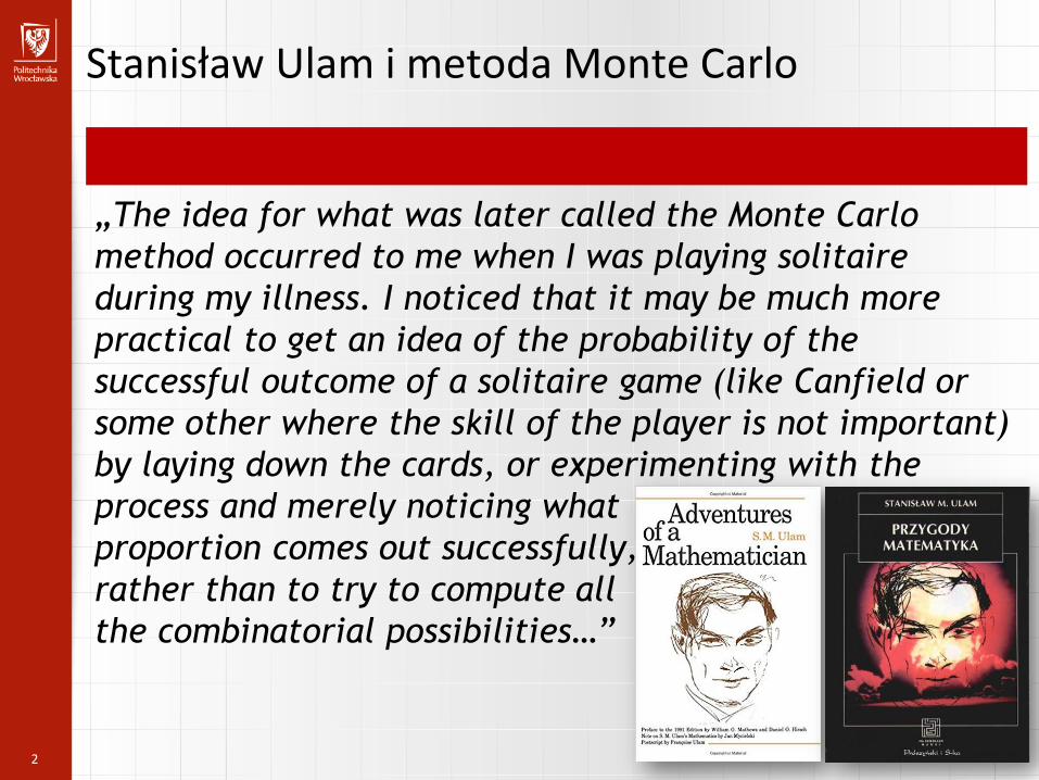
Stanisław Ulam i metoda Monte Carlo

„The idea for what was later called the Monte Carlo

method occurred to me when I was playing solitaire

during my illness. I noticed that it may be much more

practical to get an idea of the probability of the

successful outcome of a solitaire game (like Canfield or

some other where the skill of the player is not important)

by laying down the cards, or experimenting with the

process and merely noticing what

proportion comes out successfully,

rather than to try to compute all

the combinatorial possibilities…”

3

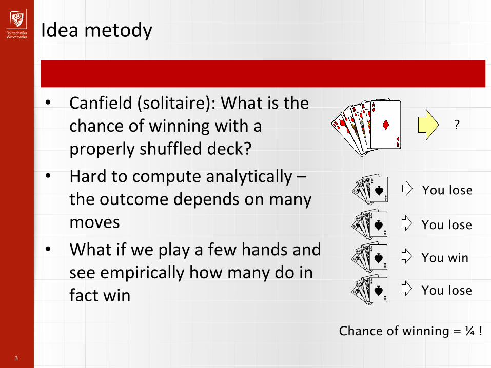
Idea metody

• Canfield (solitaire): What is the chance of winning with a properly shuffled deck?

• Hard to compute analytically –the outcome depends on many moves

• What if we play a few hands and see empirically how many do in fact win

?

You lose

You lose

You win

You lose

Chance of winning = ¼ !

4

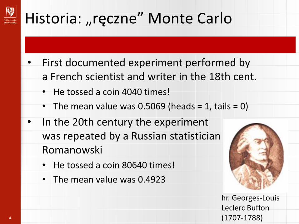
Historia: „ręczne” Monte Carlo

• First documented experiment performed bya French scientist and writer in the 18th cent.

• He tossed a coin 4040 times!

• The mean value was 0.5069 (heads = 1, tails = 0)

• In the 20th century the experiment was repeated by a Russian statisticianRomanowski

• He tossed a coin 80640 times!

• The mean value was 0.4923

hr. Georges-Louis Leclerc Buffon (1707-1788)

5

Buffon’s needle, 1733

• What is the chance that a needle randomly tossed will fall across the lines on a parquet floor?

• We randomly drop a needle of length 𝑙 < 𝑑 onto a sheet of paper with parallel lines 𝑑 apart

• Probability that a short needle crosses one of the lines:

𝑝 =2𝑙

𝜋𝑑• Show it!

Source: M. E. Calhoun, P. R. Mouton, Journal of Chemical Neuroanatomy 20 (2000) 61–69

6

Buffon’s needle, 1733

• Experiment for estimating the value of π by tossing a needle onto a ruled surface

• 𝜋 can be approximated as: 𝜋 = 2𝑛𝑙/𝑚𝑑

• where 𝑚 is the number of throws crossing a line and 𝑛is the total number of throws

Source: M. E. Calhoun, P. R. Mouton, Journal of Chemical Neuroanatomy 20 (2000) 61–69

7

How good is the approximation?

• In 1864, captain O.C.Fox performed this experiment when recovering from wounds

• Using a rotating surface improved the results –removed the bias of the “random number generator”

𝑛 𝑚 𝑙 𝑑 surface 𝜋

500 236 3 4 still 3.1780

530 253 3 4 rotating 3.1423

8

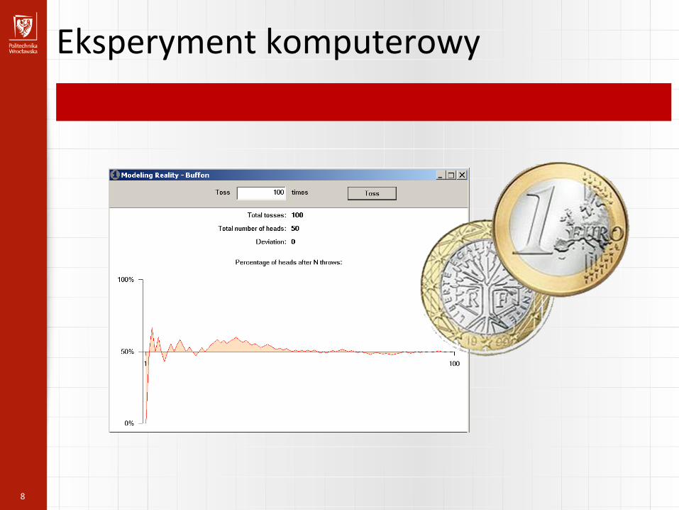
Eksperyment komputerowy

9

Pseudorandom number generator (PRNG)

A linear congruential generator

• Form a sequence 𝑈𝑛 = 𝑋𝑛/𝑚 with 𝑋𝑛+1 = 𝑎𝑋𝑛 + 𝑐 𝑚𝑜𝑑 𝑚

• All the `magic' comes from the `modulo' operator

• Goal:• producing pseudorandom numbers which can

pass formal tests for randomness• long period• fast

„magic numbers”: a, c, m are crucial

10

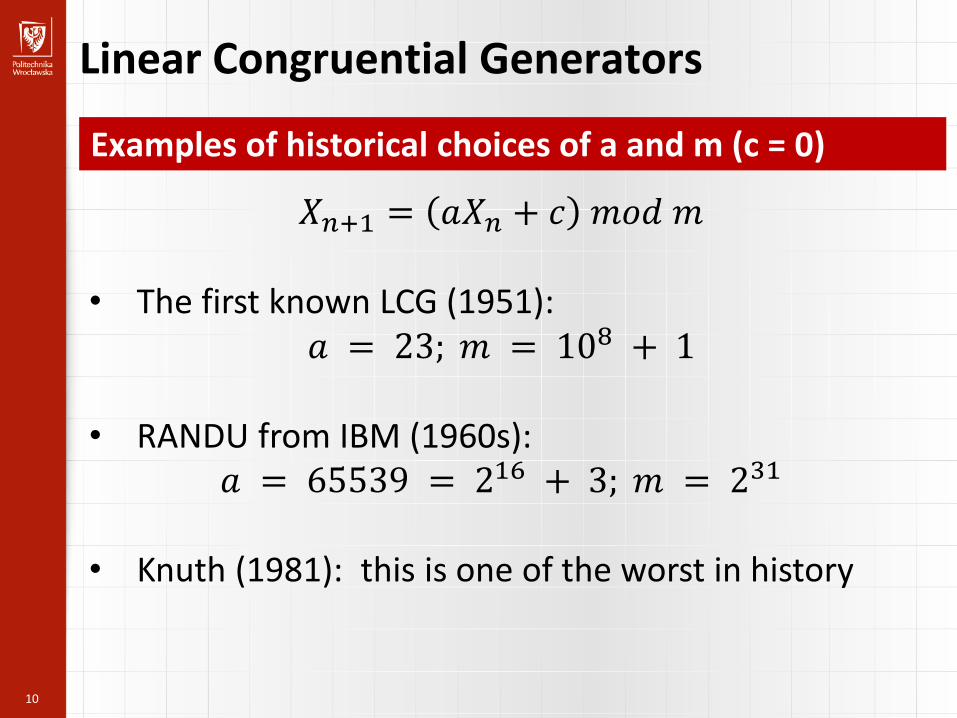
Linear Congruential Generators

Examples of historical choices of a and m (c = 0)

𝑋𝑛+1 = 𝑎𝑋𝑛 + 𝑐 𝑚𝑜𝑑 𝑚

• The first known LCG (1951): 𝑎 = 23; 𝑚 = 108 + 1

• RANDU from IBM (1960s): 𝑎 = 65539 = 216 + 3; 𝑚 = 231

• Knuth (1981): this is one of the worst in history

11

Test of IBM's RANDU generator

Do you remember the simple solution?

12

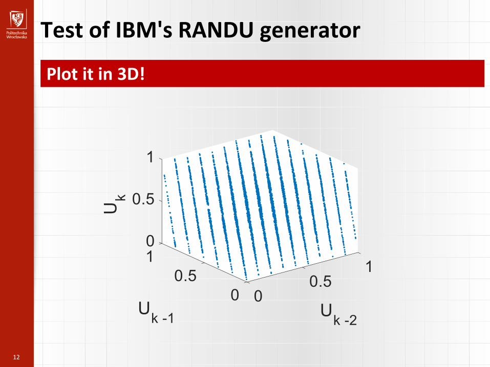
Test of IBM's RANDU generator

Plot it in 3D!

13

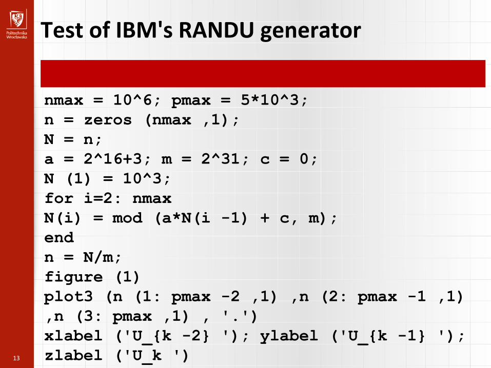
Test of IBM's RANDU generator

nmax = 10^6; pmax = 5*10^3;

n = zeros (nmax ,1);

N = n;

a = 2^16+3; m = 2^31; c = 0;

N (1) = 10^3;

for i=2: nmax

N(i) = mod (a*N(i -1) + c, m);

end

n = N/m;

figure (1)

plot3 (n (1: pmax -2 ,1) ,n (2: pmax -1 ,1)

,n (3: pmax ,1) , '.')

xlabel ('U_{k -2} '); ylabel ('U_{k -1} ');

zlabel ('U_k ')

14

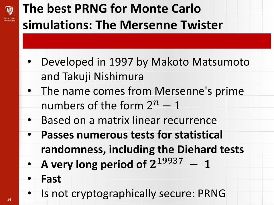
The best PRNG for Monte Carlo simulations: The Mersenne Twister

• Developed in 1997 by Makoto Matsumoto and Takuji Nishimura

• The name comes from Mersenne's primenumbers of the form 2𝑛 − 1

• Based on a matrix linear recurrence• Passes numerous tests for statistical

randomness, including the Diehard tests• A very long period of 𝟐𝟏𝟗𝟗𝟑𝟕 − 𝟏• Fast• Is not cryptographically secure: PRNG

15

3D plot for the Mersenne Twister

• Matlab ver. 7.4 and later use the MersenneTwister

16

Modern history of the MC method

• Stanisław Ulam during ... recovery from an illness plays solitaire (Canfield)

• Nicolas Metropolis gives the new method a name

• The name is a reference to the Monte Carlo casino in Monaco where Ulam’s uncle would borrow money to gamble

• In 1949 the first article about the MC method coauthored by Ulam and Metropolis is published

Stanisław Ulam (1909-1984)

17

Applications of the MC method

• Approximating probabilities

• Approximating areas of geometric figures

• Computing integrals

• Solving partial differential equations

• Weather forecasts

• Derivatives pricing

• Computing thermodynamical variables within microscopic models

• Computing aggregated variables within agent-based models

Perkolacja

© 2014 Katarzyna Sznajd-Weron

Model perkolacji (site lub bond)

• Model perkolacji :

– Każdy węzeł (wiązanie) sieci jest zajęty niezależnie z prawdopodobieństwem p

– Jak duże musi być to prawdopodobieństwo p aby powstał nieskończony?

bondsitesite

Perkolacja: Pożary lasów

21

Symulacja Monte Carlo

Source: Introduction to Computational Physics, Lecture of Prof. H. J. Herrmann

gęstość zadrzewienia pPra

wd

op

od

ob

ień

stw

o p

rzej

ścia

na

dru

gą s

tro

nę

Granica termodynamiczna:𝑁 → ∞, 𝐿 → ∞,

𝑝 =𝑁

𝐿2= 𝑐𝑜𝑛𝑠𝑡

𝐿 → ∞

Spowolnienie krytyczne (critical slowing down)

p=0.5

p=0.6

p=0.7 1 nn AND nnn 2 nn OR nnn

1 nn

23

Model perkolacji: filtry vs. pożary

Inne przykłady?

Filtr Pożar

substacja Woda/olej ogień

Płynie przez Puste miejsca Drzewa

Miejsca zakazane Ziarna/Skała Puste miejsca

P (gęstość/prawd.) Pustych miejsc Drzew

p<p* Faza sucha Faza niespalona

p>p* Faza mokra Faza spalona

24

The Burning Method

1. Label all occupied cells in the top line with the marker t=2.

2. Iteration step t+1:a) Go through all the cells and

find the cells which have label t.b) For each of the found t-label cells do

i. Check if any direct neighbor (North, East, South,West) is occupied and not burning (label is 1).

ii. Set the found neighbors to label t+1.3. Repeat step 2 (with t=t+1) until either there are no neighbors

to burn anymore or the bottom line has been reached - in the latter case the latest label minus 1 defines the shortest path.

Introduction to Computational Physics, Lecture of Prof. H. J. Herrmann

2 2

334

45

5

6

6

7

7

78

8

8

Perkolacja site

• Rozważmy sieć dwuwymiarową L na L

• Każde miejsce sieci jest zajęte niezależnie z prawdopodobieństwem p

• Klaster – grupa zajętych węzłów znajdujących się wzajemnie w najbliższym sąsiedztwie (rozmiar s)

26

Skalowanie rozmiaru (masy) klastra

ssD

ppppP

ppL

ppL

ppL

LM

cc

c

c

d

c

2

ln

Fraktal!

27

Jak zliczać klastry?

Algorytm Hoshen-Kopelman algorithm

• Lattice = matrix 𝑁𝑖𝑗,

• 𝑁 𝑖, 𝑗 = 0 (site is unoccupied)• 𝑁 𝑖, 𝑗 = 1 (site is occupied)

• 𝑀𝑘– mass of cluster 𝑘 (labels clusters)• We comb through the lattice from top-left• The algorithm is very efficient since it scales linearly with the

number of sites

28

Hoshen-Kopelman algorithmPhys. Rev. B14 (1976) 3439

1. 𝑘 = 2,𝑀𝑘 = 12. for all 𝑖, 𝑗 of 𝑁𝑖𝑗(a) if top and left are empty: 𝑘 = 𝑘 + 1,𝑁𝑖𝑗 = 𝑘,𝑀𝑘 = 1

(b) if one is occupied with 𝑘0 then 𝑁𝑖𝑗 = 𝑘0, 𝑀𝑘0 = 𝑀𝑘0 + 1

(c) if both are occupied with 𝑘1 and 𝑘2 (𝑘1 ≠ 𝑘2) then choose one, e.g. 𝑘1, 𝑁𝑖𝑗 = 𝑘1, 𝑀𝑘1 = 𝑀𝑘1 +𝑀𝑘2 +1,𝑀𝑘2 = −𝑘1(d) If both are occupied with 𝑘1, 𝑁𝑖𝑗 = 𝑘1, 𝑀𝑘1 = 𝑀𝑘1 + 1

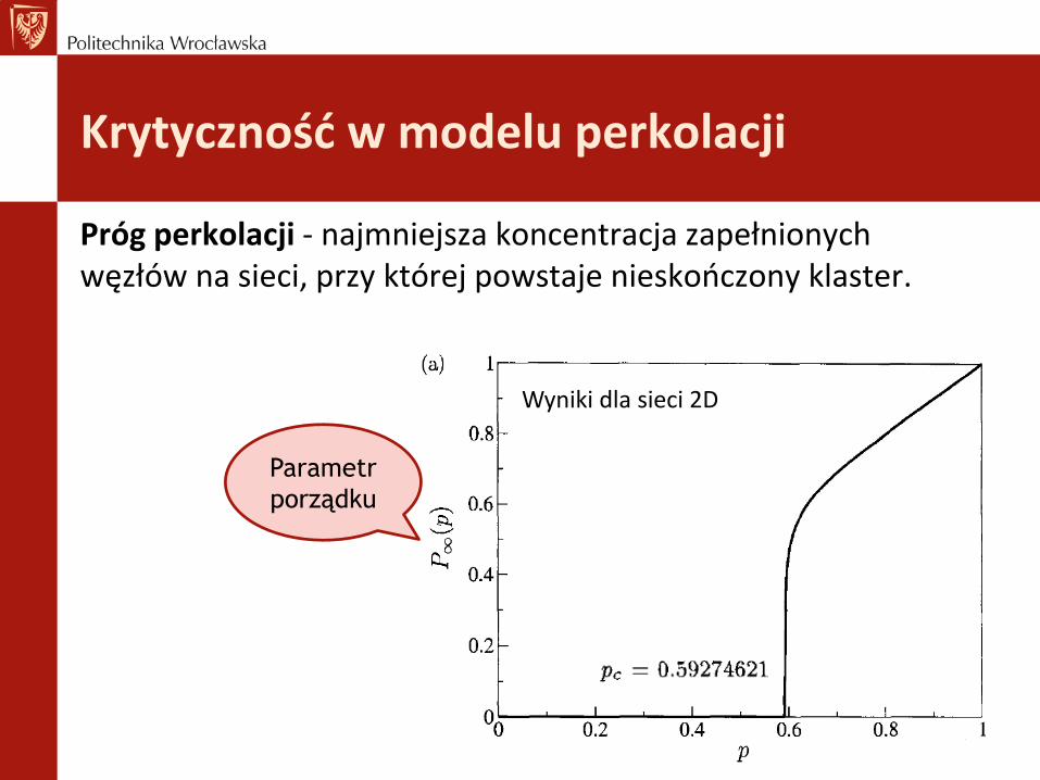
Krytyczność w modelu perkolacji

Próg perkolacji - najmniejsza koncentracja zapełnionych węzłów na sieci, przy której powstaje nieskończony klaster.

Wyniki dla sieci 2D

Parametr

porządku

Krytyczność w modelu perkolacji

• Próg perkolacji dla problemu site to najmniejsza koncentracja zapełnionych węzłów na sieci, przy której powstaje nieskończony klaster.

• Próg perkolacji dla problemu bond to najmniejsza koncentracja zapełnionych połączeń między węzłami sieci, przy której powstaje nieskończony klaster.

Próg perkolacji nie jest uniwersalny!

sieć site bond

heksagonalna 0.696 2 0.652 71

kwadratowa 0.592 75 0.500 00

trójkątna 0.500 00 0.347 29

diamond 0.428 0.388

Prosta

kubiczna

0.311 7 0.249 2

BCC 0.245 0.178 5

FCC 0.198 0.119

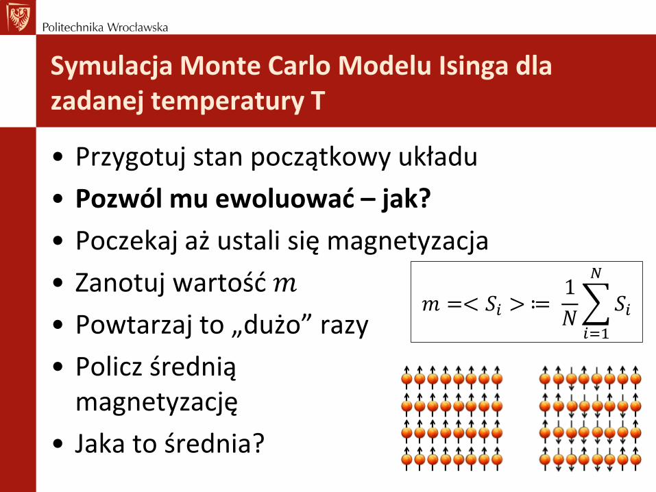
Symulacja Monte Carlo Modelu Isinga dla zadanej temperatury T

• Przygotuj stan początkowy układu

• Pozwól mu ewoluować – jak?

• Poczekaj aż ustali się magnetyzacja

• Zanotuj wartość 𝑚

• Powtarzaj to „dużo” razy

• Policz średnią magnetyzację

• Jaka to średnia?

𝑚 =< 𝑆𝑖 >≔1

𝑁

𝑖=1

𝑁

𝑆𝑖

Średnia po czasie

Śred

nia

po

zes

po

le

Średnia po czasie i średnia po zespole

Układ ergodyczny to średnia po zespole = średnia po czasie

Algorytm Metropolisa

Algorytm Metropolisa – 1MCS = N losowań

• Wylosuj jeden spin 𝑆𝑖

• Oblicz energię E = 𝐸(𝑆𝑖) = −𝑆𝑖𝐽 σ𝑗∈𝑛𝑛 𝑆𝑗

• Oblicz energię E′ = 𝐸(−𝑆𝑖) = 𝑆𝑖𝐽 σ𝑗∈𝑛𝑛 𝑆𝑗

• Oblicz zmianę energii ΔE = E′ − E

• Jeżeli ΔE ≤ 0 to 𝑆𝑖 → −𝑆𝑖• Jeżeli ΔE > 0 to wylosuj 𝑟 z przedziału [0,1] i akceptuj

nową konfigurację jeżeli:

𝑟 < 𝑝 = 𝑒𝑥𝑝 −Δ𝐸

𝑘𝐵𝑇, 𝑘𝐵 = 𝐽 = 1

Wylosuj spin 𝑆𝑖

Oblicz Δ𝐸obrotu 𝑆𝑖 → −𝑆𝑖

Δ𝐸 < 0? Wylosuj 𝑥 ∼ 𝑈(0,1)Obróć spin𝑆𝑖 → −𝑆𝑖

TAK NIE

𝑥 < exp(−Δ𝐸/𝑇)?Obróć spin𝑆𝑖 → −𝑆𝑖

TAK NIE

𝑖𝑡𝑒𝑟 ≥ 𝑁?

Oblicz magnetyzację

TAKNIE

Trajektorie dla T=1.85, L=100 (symulacje Jakub Pawłowski)

Trajektorie dla T=2.26(symulacje Jakub Pawłowski)

Przejście fazowe w modelu Isinga(symulacje Maciej Tabiszewski)

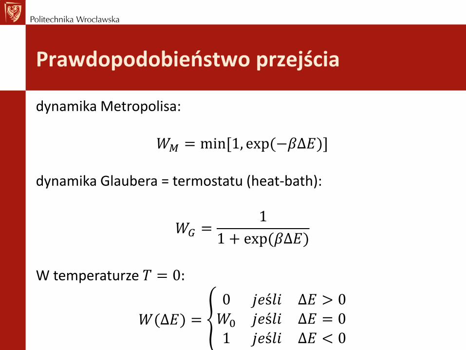
Prawdopodobieństwo przejścia

dynamika Metropolisa:

𝑊𝑀 = min[1, exp(−𝛽Δ𝐸)]

dynamika Glaubera = termostatu (heat-bath):

𝑊𝐺 =1

1 + exp(𝛽Δ𝐸)

W temperaturze 𝑇 = 0:

𝑊(Δ𝐸) = ൞

0 𝑗𝑒ś𝑙𝑖 Δ𝐸 > 0𝑊0 𝑗𝑒ś𝑙𝑖 Δ𝐸 = 01 𝑗𝑒ś𝑙𝑖 Δ𝐸 < 0

Dynamiki w modelu Isinga

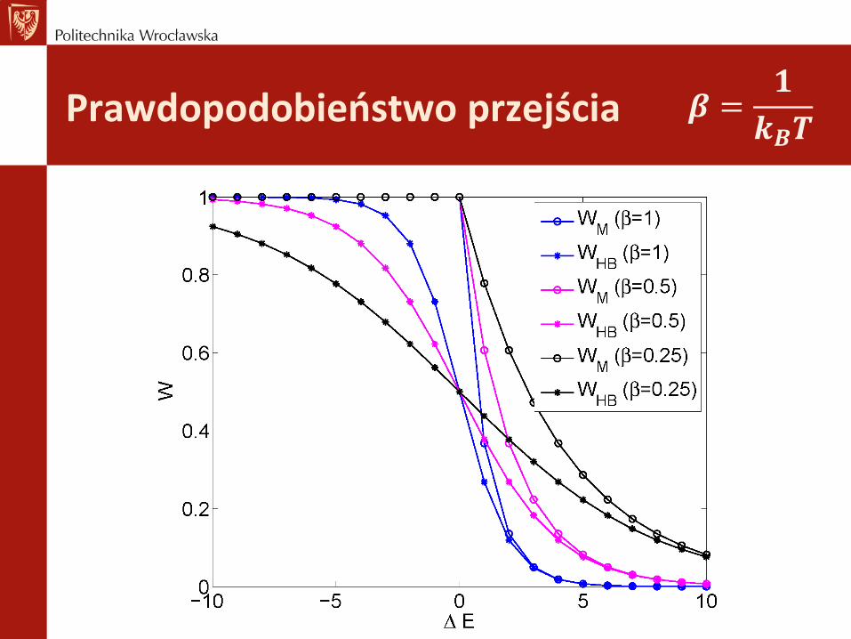
Prawdopodobieństwo przejścia 𝜷 =𝟏

𝒌𝑩𝑻

Ewolucja gęstości prawdopodobieństwa

𝑑𝑃𝑟𝑑𝑡

=

𝑠≠𝑟

𝑊𝑠→𝑟𝑃𝑠 −

𝑠≠𝑟

𝑊𝑟→𝑠𝑃𝑟

𝑑𝑃𝑟𝑑𝑡

=

𝑠≠𝑟

𝑊𝑠→𝑟𝑃𝑠 −𝑊𝑟→𝑠𝑃𝑟 = 0

𝑾𝒔→𝒓𝑷𝒔 = 𝑾𝒓→𝒔𝑷𝒓

𝑷𝒓 = 𝒁𝒆𝒙𝒑 −𝜷𝑬𝒓

𝑾𝒔→𝒓

𝑾𝒓→𝒔=𝑃𝑟𝑃𝑠=𝑍𝑒𝑥𝑝 −𝛽𝐸𝑟𝑍𝑒𝑥𝑝 −𝛽𝐸𝑆

= 𝐞𝐱𝐩(−𝜷𝚫𝑬)

Warunek stacjonarności

Warunek równowagi szczegółowej

Rozkład w równowadze

Rozkład magnetyzacji w czasie dla T=1.85(symulacje Jakub Pawłowski)

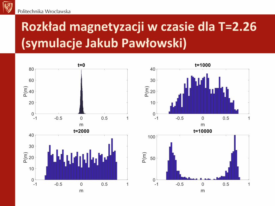
Rozkład magnetyzacji w czasie dla T=2.26(symulacje Jakub Pawłowski)

Relaksacja w T=0 z aktualizacją sekwencyjną

Literatura

• D. W. Heermann, Podstawy symulacji komputerowych w fizyce, WNT 1997

• D. P. Landau, K. Binder, A Guide to Monte Carlo Simulations in Statistical Physics, Cambridge University Press 2005

• Klaster perkolujący – rozciąga się w nieskończoność

• Rozważmy spacer po perkolującym nieskończonym klastrze

• Kontynuując spacer z węzła 𝑖-tego możemy pójść w 𝑧 − 1 kierunkach

• Tylko 𝑝(𝑧 − 1) jest wolnych

• Czyli musi być przynajmniej jedna wolna

• 𝑝 𝑧 − 1 ≥ 1 → 𝑝𝑐 =1

𝑧−1

Trzewo (sieć) Bethego (z=3)

Perkolacja na sieci kwadratowej (bond): dualność sieci

mogę przejść

nie mogę przejść

p

q=1-p

Sieć wyjściowa:

nie mogę przejść

mogę przejść

p

q=1-p

Sieć dualna:

5.0*

***,1*

**

**

p

pqpq

qqpp

qqpp

Samodualność sieci kwadratowej

Metoda Średniego Pola (MFA) – perkolacja wiązań (bond)

• Pytanie: Jaka jest krytyczna wartość koncentracji wiązań (mostów), przy której powstanie nieskończony klaster?

• Oznaczenia:

– prawdopodobieństwo tego, że dwa dowolne węzły sieci są połączone (tzn. że istnieje wiązanie): 𝑝

– prawdopodobieństwo, że 𝑖-ty węzeł należy do nieskończonego klastra: P𝑖

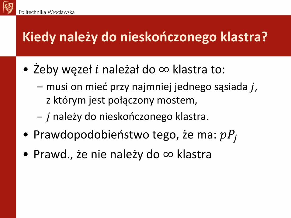
Kiedy należy do nieskończonego klastra?

• Żeby węzeł 𝑖 należał do ∞ klastra to:

– musi on mieć przy najmniej jednego sąsiada 𝑗, z którym jest połączony mostem,

– 𝑗 należy do nieskończonego klastra.

• Prawdopodobieństwo tego, że ma: 𝑝𝑃𝑗

• Prawd., że nie należy do ∞ klastra

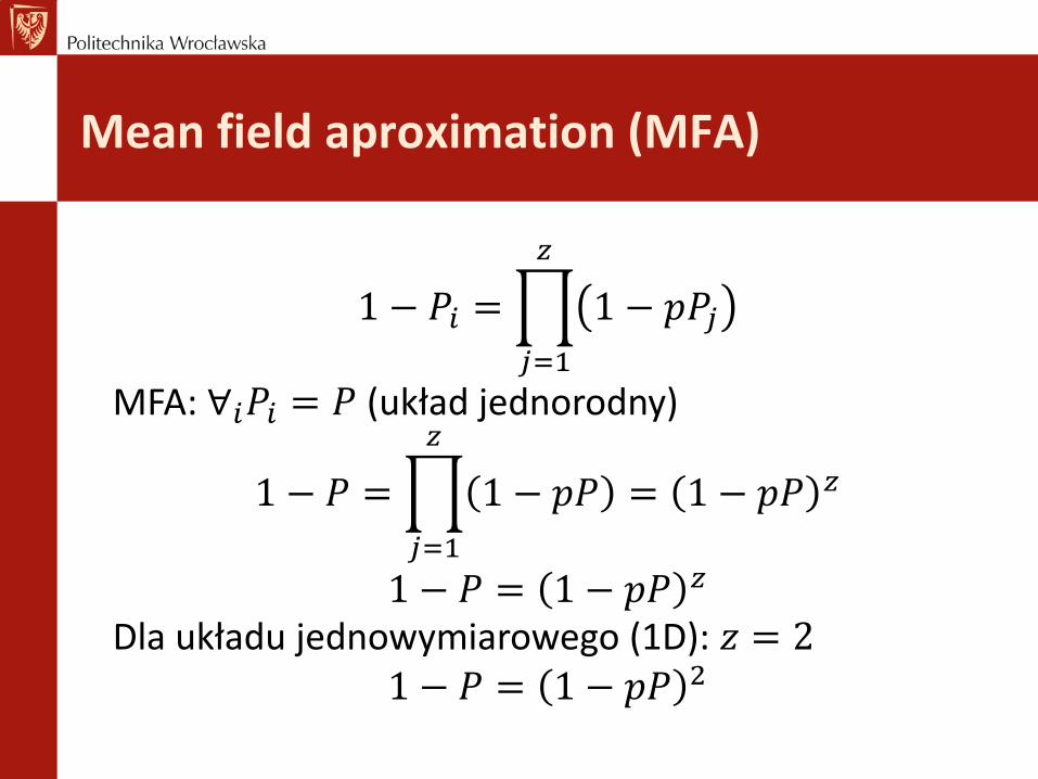
Mean field aproximation (MFA)

1 − 𝑃𝑖 =ෑ

𝑗=1

𝑧

1 − 𝑝𝑃𝑗

MFA: ∀𝑖𝑃𝑖 = 𝑃 (układ jednorodny)

1 − 𝑃 =ෑ

𝑗=1

𝑧

1 − 𝑝𝑃 = 1 − 𝑝𝑃 𝑧

1 − 𝑃 = 1 − 𝑝𝑃 𝑧

Dla układu jednowymiarowego (1D): 𝑧 = 21 − 𝑃 = 1 − 𝑝𝑃 2

Układ jednowymiarowy, 𝑧 = 2

1 − 𝑃 = 1 − 𝑝𝑃 2

Pytanie: Czy istnieje takie 𝑝, żeby 𝑃 > 0?

1 − 𝑃 = 1 − 2𝑝𝑃 + 𝑝2𝑃2

𝑝2𝑃2 + 1 − 2𝑝 𝑃 = 0𝑃(𝑝2𝑃 + 1 − 2𝑝 ) = 0

𝑝2𝑃 + 1 − 2𝑝 = 0 → 𝑃 =2𝑝 − 1

𝑝2

𝑃 =2𝑝 − 1

𝑝2> 0 → 2𝑝 − 1 > 0 → 𝑝 >

1

2

p

p’

42

3

22

4

2

)1(4

)1(2

'

pp

pp

pp

pp

Grupa renormalizacyjna (decymacja): Perkolacja na sieci kwadratowej

p=0 p’=0 p’’=0 …

p=1 p’=1 p’’=1 …

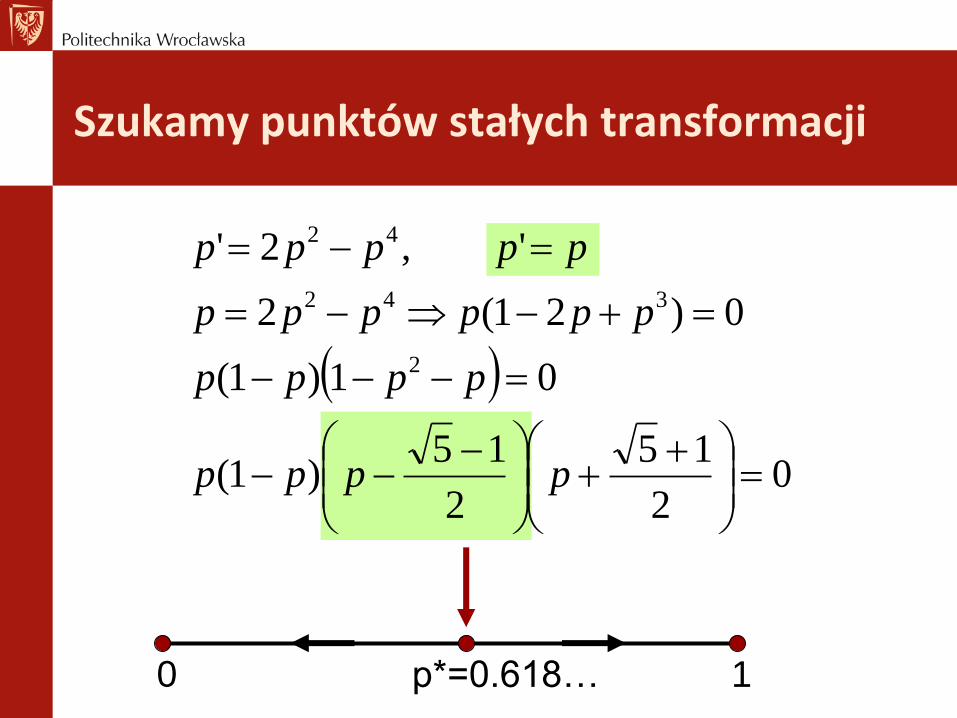
02

15

2

15)1(

01)1(

0)21(2

',2'

2

342

42

pppp

pppp

pppppp

ppppp

0 p*=0.618… 1

Szukamy punktów stałych transformacji

Grupa renormalizacyjna (majority rule): Perkolacja na sieci trójkątnej

𝑝 – prawdopodobieństwo𝑝′ – prawdopodobieństwo𝑝′ = 𝑝3 + 3𝑝2 1 − 𝑝

𝑝′ = 𝑝𝑝 = 𝑝3 + 3𝑝2 1 − 𝑝

−2𝑝3 + 3𝑝2 − 𝑝 = 0𝑝(−2𝑝2 + 3𝑝 − 1) = 0

𝑝 1 − 𝑝1

2− 𝑝 = 00 𝑝𝑐 =

1

21