Nikolaus H. R. Howe

Abstract

In this paper, we propose a technique to identify the absolute timing information (T0) of any inter-action in the MicroBooNE detector. We achieve this by means of a point-matching technique. A singlepoint is assigned to each interation recorded by the PMTs by using energy and position information.Similarly, a single point is assigned to each interaction recorded by the TPC by weighting by energy anddistance to detector. Finally, these points are matched based on their position. Aquisition of timinginformation allows us to reconstruct the absolute 3D position of an interaction in the detector, which isessential for event visualization and removal of cosmic ray data.

Introduction

MicroBooNE is an experiment on the Booster Neutrino Beamline (BNB) at Fermilab which studies the quan-tum mechanical phenomenon on neutrino oscillation. The characteristics of this oscialltion are determined bythe differences between different non-zero neutrino masses. The most accepted description of neutrino oscilla-tion involves only 3 different mass eigenstates, but MicroBooNE seeks for a possible fourth mass eigenstate bymeasuring a flavour oscillation of a muon type neutrino into an electron type neutrino. The neutrino sourcefor the experiment is the BNB at Fermilab, which produces a high purity muon type neutrino beam. Theexperiment employs a Liquid Argon Time Projection Chamber (LArTPC) to identify neutrino interactionswith Argon nuclei in the detector. The LArTPC allows us to obtain high resolution images of the paths ofcharged particles inside the decetor, and provides rich calorimetric information together with detailed dE/dxalong a particle’s trajectory points. Particles’ topology and interaction classification is particularly importantfor distinguishing a real electron type neutrino signal, which creates an electron, against backgrounds suchas cosmic ray muons, muon type neutrinos and such.

Starting Out

The first data used in this study were mc-simulated single muon tracks (one per event). Each event contains anumber of flashes. We first try plotting the differences in the flash z and y position with the truth informationwe get from Monte Carlo (mc) data. Plots of these differences can be seen in Figures 1 and 2.

1

Nikolaus H. R. Howe

Figure 1: Difference in truth and flash recon-structed y position.

Figure 2: Difference in truth and flash recon-structed z position.

In the y direction we note an almost flat distribution ranging from −116cm to +116cm (the height of thedetector). This gives us little information on the vertical position of the interaction to which these flashesare matched. The z direction appears more promising: there is a peak around 0 and the graph has a sharppeak at 0, suggesting that the distribution may be made up of two or more distributions. If we can find someway to isolate the central distribution, that would provide useful position information from the flash z PMTinformation.

This plot reveals a couple of other noteworthy points. First, there are ∼ 106 entries in the histogram,but only ∼ 104 events. Dividing number of entries by number of events, we estimate there should be ∼ 40

flashes per event. A rough estimate of the area under the ‘tighter curve’ suggests no more than a few tensof thousands of entries. Since there are ten thousand events, this suggests that each event has no more thana few ‘useful’ flashes (the rest are noise). Before we attempt to isolate these useful flashes, however, let uspause to make sure we understand what is happening in the detector itself, with reference to Figure 2.

Figure 3: 2D picture of first event in detector. Figure 4: 2D picture of second event in detector.

2

Nikolaus H. R. Howe

Figure 5: 2D picture of third event in detector. Figure 6: 2D picture of fourth event in detector.

Figures 3 through 6 show graphical represntations for the y-z plane of the first four (of ten thousand)simulated events. The x axis shows the logitudinal detector direction; the y axis shows the vertical direction.The green and red points represent the truth start and end poisition of the interaction. Each blue dotrepresents a flash received by the PMTs. It is clearly visible that many, if not most, of the flashes do notcarry accurate position information. We may still obtain useful information from the flashes—we just needsome way to separate data from noise. Since we are working with PMTs, whose reliability improves themore photoelectrons are recorded∗, we try choosing only flashes that make a certain energy cut. For no goodreason†, we choose the cut value to be 5 photoelectons (PE).

Figure 7: 2D picture of event 0 in detector with5PE cut.

Figure 8: 2D picture of event 1 in detector with5PE cut.

∗I’ll come back to this†I’ll come back to thiso ne too....

3

Nikolaus H. R. Howe

Figure 9: 2D picture of event 2 in detector with5PE cut.

Figure 10: 2D picture of event 3 in detector with5PE cut.

With the 5PE cut, not only is the number of points per event reduced in most cases to one or two, but theremaining points fall very close to the truth start and end, at least in the z direction (we weren’t expectingmuch from the y direction anyway). Table 1 shows the breakdown of number of points per event which makethe cut.

# flashes # events0 681 91822 6943 454 9

> 4 1

Table 1: Number of flashes per event after 5PE cut.

As seen in Table 1, the vast majority of events (blue) now have only flash. This puts us well on ourway to having a single point per event in the detector, which we will need in order to assign a T0 to eachTPC-reconstructed event. About 7% of the data, however (red) still have more than one point. We willaddress this problem later—for now, let us take a step back and remind ourselves of the overarching processof which this is a part‡.

Overall Procedure

So far we have concerned ourselves with flash data, but our overall goal of finding T0 for any interactioninvolves more than PMT analysis. With reference to Figure 12, we now outline the overarching procedure.‡The 68 events with no flashes above 5PE actually had no interaction within the detector, and hence have no flash above the

cut value.

4

Nikolaus H. R. Howe

Figure 11: Workflow schematic.

On the right side, we see the PMT side of things. Once we have a list of candidate flashes (providedby the 5PE cut) for each event, we need some way to assign a single flash-point to each interaction. Thisis managed by the Flash Selection Algorithm, which we will examine in more detail later. The TPC sideoccupies the left portion of the flowchart. Using a Point Estimator Algorithm, which we will also describelater, we assign a point to each reconstructed track. Finally, with the Flash Match Algorithm, we match thePMT and TPC points, so that every interaction has a T0. We now examine the Flash Selection algorithm.

PMT Points

As seen earlier, when we cut at 5PE, we eliminate most of the noise, but many events still have more thanone flash. Since we need a single point per interaction, we must reduce this number to one flash per event.Before we address this problame, let us examine the energy spectrum of each event.

Figure 12: PE values of all flashes in event 0. Figure 13: PE values of all flashes in event 1.

5

Nikolaus H. R. Howe

Figure 14: PE values of all flashes in event 2. Figure 15: PE values of all flashes in event 3.

As shown in Figures 13 through 16, every event seems to have one single flash with much greater energythan the rest. We also note that every one of these ‘max points’ occurs very soon after the trigger time (i.e.just after 0 on the time axis). Since the interaction likely releases the greatest amount of energy in its firstinteraction§, and the ‘first interaction’ occurs at trigger time, we take the maximum #PE value point in eachevent as a good way, at least initially, to assign a single point to each interaction. The diagrams also explainwhy the 5PE cut did such a good job of reducing noise: all noise seems to occur at ∼ 3PE.

Finding the best cut value

The cut value of 5PE did an initial good job of removing noise and isolating useful data. It was, however,chosen somewhat arbitrarily, and we should check other values to see if we get better results. In Figure 13,we examine the effect of different #PE values, which range on the x axis from 5 to 100PE.

Figure 16: Width of histogram and efficiency for different cut values.

Figure 11 shows that even as #PE approaches 100, the width of the histogram (blue) does not changemuch. The efficiency (red), which measures the amount of available data that was actually used in the§I guess it would be good to explain why this is

6

Nikolaus H. R. Howe

analysis, decreases significantly. Thus, we decide that the preliminary cut of 5PE is, for the time being, agood cut value, as it is high enough to remove most noise (which occurs around 3PE), yet low enough tomaintain ∼ 99% efficiency.

Dealing with multiple-interaction events

We must address one final problem: how to approach events that have multiple interactions, and thereforemultiple valid flashes. We do so by using an algorithm called MaxNPEWindow. We now examine how thealgorithm works with reference to Figure 17.

Figure 17: Illustration of Event Analysis with MaxNPEWindow.

First, all flashes in an event are ordered in terms of #PE. Flashes are then looped over from higher tolower PE value. A window is opened in time¶ around the first flash. If the next flash falls within the window,it is ignored; if it does not, then a new window is opened around it. The algorithm continues in such a fashionuntil the PE cut value is reached.

Now that we have a way to assign PMT points, we shift our focus to methods for finding a TPC pointper interaction. We will do so with the QWeightPoint algorithm, with reference to the diagram in Figure 18.

Figure 18: Illustration of Event Analysis with QWeightPoint.

TPC Points

The diagram in Figure 18 represents a single particle track in the detector, broken into segments during whichthe particle was travels without changing direction (in reality these will be on the ∼ 3mm scale). First, thealgorithm finds the midpoint of each segment, and assigns to it the difference in energy between its endpoints.¶an upgrade to this algorithm would open the window in z-space as well

7

Nikolaus H. R. Howe

Now, we want to ultimately match this point to our PMT point, so we need a way to get the energy levelsbehaving similarly to as they would with a PMT. We know that the intensity read by a PMT drops off asr−2, so we divide each energy-weighted midpoint of our TPC track, the distance to the detector squared.This leaves us with a number of weighted midpoints, but we ultimately want a single point per interaction.To reduce these to a single point, we take the average position of the midpoints in y and z, weighted by thedistance-weighted value found earlier.

While our technique seems reasonable, does it give good results? In Figure 18, we compare the resolutionof results obtained from two different TPC point-finding techniques.

Figure 19: Comparison of resolution with old (start point) vs new (QWeightPoint) TPC point-finding tech-niques.

The red histogram is constructed by taking the difference in MC start position and the z position of theflash-with-max-PE point. The blue histogram shows a similar difference, but in place of MC start, uses thenew technique for reconstructing the point. The plot strongly suggests that, with a tighter width around 0and a higher peak, this new technique does a better job than the simple one we were using before.

Matching Points

Now that we have methods to find both the PMT and TPC points, we can finally combine them to achieveour goal of finding a T0 for every interaction. The most immediate method is simply to match points basedon position. This process is outlined in Figure 20.

8

Nikolaus H. R. Howe

Figure 20: Matching PMT and TPC points.

First, all points in an event are ordered in #PE. Then, looping over the points from greatest to least#PE, each PMT point is assigned to the TPC point that is closest to it in the z direction (remember that wefound earlier that the y information is not very reliable). The process is continued until no points remain.

Cosmic Analysis

Of course, our analysis does not end with a single muon track—real neutrino beams will be much morecomplex. The next step in our analysis is to examine how well our algorithms perform with cosmic events.We now analyze a number of events, each of which contain not only multiple tracks per interaction, but alsomultiple interactions per event.

To start off our analysis, we find the difference in Z position between our reconstructed points and truthinformation, just as with the single muon track.

Figure 21: Z flash position for cosmics.

As shown in Figure 21, our algorithms translate very well from the single-track to the cosmic events. Wehave a nice peak centered around 0, with a width of ∼50cm.

Now, our primary goal in this study is T0 reconstruction. Given that our matching algorithm dependson Z position accuracy, we expect that our T0 matching should also be accurate. To test this expectation,we plot difference in truth and reconstructed time in Figure 22.

9

Nikolaus H. R. Howe

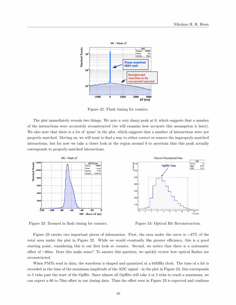
Figure 22: Flash timing for cosmics.

The plot immediately reveals two things. We note a very sharp peak at 0, which suggests that a numberof the interactions were accurately reconstructed (we will examine how accurate this assumption is later).We also note that there is a lot of ‘grass’ in the plot, which suggests that a number of interactions were notproperly matched. Moving on, we will want to find a way to either correct or remove the improperly-matchedinteractions, but for now we take a closer look at the region around 0 to ascertain that this peak actuallycorresponds to properly-matched interactions.

Figure 23: Zoomed in flash timing for cosmics. Figure 24: Optical Hit Reconstruction.

Figure 23 carries two important pieces of information. First, the area under the curve is ∼47% of thetotal area under the plot in Figure 22. While we would eventually like greater efficiency, this is a goodstarting point, considreing this is our first look at cosmics. Second, we notice that there is a systematicoffset of ∼60ns. Does this make sense? To answer this question, we quickly review how optical flashes arereconstructed.

When PMTs read in data, the waveform is shaped and quantized at a 64MHz clock. The time of a hit isrecorded as the time of the maximum amplitude of the ADC signal—in the plot in Figure 24, this correspondsto 5 ticks past the start of the OpHit. Since almost all OpHits will take 4 or 5 ticks to reach a maximum, wecan expect a 60 to 70ns offset in our timing data. Thus the offset seen in Figure 23 is expected and confirms

10

Nikolaus H. R. Howe

our understanding of the region around 0.

Conclusion

In this paper we have examined how to find a T0 for any interaction in MicroBooNE (or any comparableLArTPC detector). By taking a 5PE cut, and then finding the maximum-#PE flash per event, we identifieda single PMT-point per interaction. Using our QWeightPoint algorithm, we identified a single TPC-pointper interaction. Finally, we matched them up to find our T0. The specific software used for this study is notparticularly important: rather, we care that we now have an effective, modular system that can be upgradedas needed, piece by piece.

One potential upgrade would be in our TPC-point identification. The move to weighting by distancesquared helped immensely, but other considerations could improve our data even more. One such thoughtis that, while the TPC is a plane, the PMT array is better thought of as a number of points. Thus,distance calculations from PMTs are not as simple as dropping the normal to the y-z plane, which is thecurrent distance-weighting techinque. A more advanced TPC-point weighting technique would take intoconsideration the positions of the individual PMTs, and weight not based on distance to the plane, but tosome subset of the PMT array (for example, to the 8 closest PMTs). In this way, it is expected that the PMTinformation would match up even more precisely to the TPC points, allowing for more precise T0 assignmentand event reconstruction.

Our PMT-point algorithm could also be improved. The current algorithm opens a window in time aroundthe flash point, but we could do a better job if we also opened a window in space, thus greatly reducing thechance of losing multiple interactions that occured at similar times.

Finally, it is worth mentioning that it would be nice to have some Y position information. While addressingother issues may lead to greater reliability of the proposed matching technique, it seems that finding a way toget useful position information in the Y direction (even if somewhat inaccurate) could provide more positionalcertainty and again help improve matching.

11