Mixed-scale Jump Regressions with Bootstrap Inference∗

Jia Li,† Viktor Todorov,‡ George Tauchen§ and Rui Chen¶

January 2, 2016

Abstract

We develop an efficient mixed-scale estimator for jump regressions using high-frequency assetreturns. A fine time scale is used to accurately identify the locations of large rare jumps inthe explanatory variables such as the price of the market portfolio. A coarse scale is then usedin the estimation in order to attenuate the effect of trading frictions in the dependent variablesuch as the prices of potentially less liquid assets. The proposed estimator has a non-standardasymptotic distribution that cannot be made asymptotically pivotal via studentization. Wepropose a novel bootstrap procedure for feasible inference and justify its asymptotic validity.We show that the bootstrap provides an automatic higher-order asymptotic approximation byaccounting for the sampling variation in estimates of nuisance quantities that are used in ef-ficient estimation. The Monte Carlo analysis indicates good finite-sample performance of thegeneral specification test and confidence intervals based on the bootstrap. We apply the methodto a high-frequency panel of Dow stock prices together with the market index defined by theS&P 500 index futures over the period 2007–2014. We document remarkable temporal stabil-ity in the way that stocks react to market jumps. However, this relationship for many of thestocks in the sample is significantly noisier and more unstable during sector-specific jump events.

Keywords: bootstrap, high-frequency data, jumps, regression, semimartingale, specificationtest, stochastic volatility.

JEL classification: C51, C52, G12.

∗We thank the guest editors and anonymous referees as well as Torben Andersen, Snehal Banerjee, Tim Bollerslev,Anna Cieslak, Silvia Goncalves, Andrew Patton and Brian Weller for helpful discussions and comments. We alsothank Rob Engle and other participants of the 6th French Econometrics Conference celebrating Professor Gourieroux’sContribution to Econometrics. Li’s and Todorov’s research have been partially supported by NSF grants SES-1326819and SES-0957330, respectively.†Department of Economics, Duke University, Durham, NC 27708; e-mail: jl410@duke.edu.‡Department of Finance, Kellogg School of Management, Northwestern University, Evanston, IL 60208; e-mail:

v-todorov@northwestern.edu.§Department of Economics, Duke University, Durham, NC 27708; e-mail: george.tauchen@duke.edu.¶Department of Economics, Duke University, Durham, NC 27708; e-mail: rui.chen@duke.edu.

1 Introduction

The availability of high-frequency data has led to new ways of estimating an asset’s exposures

to systematic risks such as the aggregate stock market return in the standard CAPM. The high-

frequency estimation approach (Andersen, Bollerslev, Diebold, and Vega (2003); Barndorff-Nielsen

and Shephard (2004a); Andersen, Bollerslev, Diebold, and Wu (2006); Mykland and Zhang (2009))

uses realized variation measures to infer beta over a fixed period of time, usually a day or a month,

and then tracks these estimates over non-overlapping sample periods. More recent practice is to

conduct estimation using jump-robust measures of variation and covariation (Todorov and Boller-

slev (2010); Gobbi and Mancini (2012)). All of the above mentioned beta measures (with or without

truncation) mainly pertain to the locally Gaussian diffusive moves in the market, because the large

number of small diffusive moves are known to account for a major part of the market variation.

Economically speaking, these small moves in part reflect the market’s gradual price discovery pro-

cess of distilling minor news on fundamentals from noise trading (Kyle (1985)) which can lead to

a situation with low signal to noise ratio and temporal instability.1 Li, Todorov, and Tauchen

(2014), on the other hand, suggest an opposite approach that mainly uses abrupt and locally large

jump moves to generate an effective measure of beta.2,3 Such moves are typically related to impor-

tant market-wide shocks which include, but are not limited to, macro announcements, geopolitical

events and natural disasters. [See Chapter 8 of Hasbrouck (2015) for more discussion.]

The use of large rare jumps in a regression setting requires new ways of thinking about regression

and inference. On the one hand, in any given fixed span of time, there are only a finite number

of jumps. This means that the number of informative observations in a jump regression is finite

and does not increase to infinity asymptotically.4 Therefore, the common intuition underlying the

law of large numbers does not apply here. On the other hand, we recognize that the jumps are of

fixed size regardless of the sampling frequency, whereas the diffusive moves are on the order ∆1/2n ,

where ∆n is the sampling interval which goes to zero asymptotically. The diffusive moves in the

1Indeed, Kalnina (2013) and Reiss, Todorov, and Tauchen (2015) document that spot betas remain constant onlyover very short periods of time, usually a week or, at best, a month.

2Jump betas have been first introduced in Todorov and Bollerslev (2010). Todorov and Bollerslev (2010) usehigher order power variations to identify the jump betas from the high-frequency data. This approach, unlike Li,Todorov, and Tauchen (2014), makes use of all of the high-frequency increments. Of course, the role of the incrementswithout jumps vanishes asymptotically in the higher order power variations.

3Theoretically, the betas at jump and non-jump times do not need to coincide.4Even if the asset price process has infinitely active jumps, the number of jumps that have sizes greater than any

fixed level remains finite.

2

vicinity of jumps can be viewed as measurement errors induced by discrete sampling, and they

play the role of random disturbances in classical regressions. The magnitude of such measurement

error shrink at the parametric rate with well-behaved asymptotic properties, which can be further

used for studying the asymptotics of our estimators. In the same vein, the correct specification of

a linear jump regression model amounts to a perfect fitting (i.e., R2 = 1) of the dependent jumps

in the continuous-time limit. This test can be carried out by examining whether the observed R2

is statistically significantly below unity.

This paper develops a new mixed-scale strategy for jump regressions, which addresses a natural

asymmetry between the explanatory and dependent variables seen in applications.5 On the one

hand, the explanatory variables are often returns of highly liquid assets such as market index

futures. We sample these variables at a fine scale, which greatly improves the accuracy of jump

detection. On the other hand, the dependent variables are typically returns of less liquid assets

such as individual stocks, which are subject to a slower price discovery process for incorporating

new information. Realistically speaking, due to the trading mechanisms on the exchanges, a jump

typically cannot be observed instantly. Rather, it needs to be realized through a sequence of

transactions. See Barndorff-Nielsen, Hansen, Lunde, and Shephard (2009) for a discussion of what

they term “gradual jumps.” It is therefore prudent to sample these asset prices at a coarse scale

when estimating the jump regression model, at the cost of statistical efficiency. The mixed-scale

approach provides a flexible way of using data that play distinct roles in the jump regression. The

fact that the jump detection step and the jump regression step are performed under two (possibly)

distinct scales also leads to novel asymptotic results (cf. Li, Todorov, and Tauchen (2014)). In

addition, we present all theory here in a multivariate setting so as to facilitate applications to

multi-factor models of risk exposure.

Compared to Li, Todorov, and Tauchen (2014), an additional key econometric contribution

of the current paper is to provide a bootstrap method for conducting feasible inference for the

mixed-scale jump regression. We show that the bootstrap is asymptotically valid. Moreover, the

bootstrap provides a conceptually different alternative to the refined inference in Li, Todorov, and

Tauchen (2014). The latter is based on direct higher-order asymptotic approximations while the

current bootstrap method is aimed at approximating the finite sample distribution of the estimator

using simulated data. Our motivation for using the bootstrap is that the asymptotic distribution of

5Our mixed-scale strategy is designed to improve the accuracy of jump detection for a subvector of a multivariatesemimartingale process, so the goal here is to reduce the misclassification (i.e., jump or non-jump) error. This isfundamentally different from the multi-scale method of Zhang, Mykland, and Aıt-Sahalia (2005), which conducts ajackknife bias-correction using realized variances computed at subsamples with different frequencies in the estimationof integrated volatility.

3

the estimator of jump beta is non-standard because volatility may co-jump at the jump times of the

explanatory variable(s); see, for example, Jacod and Todorov (2010), Todorov and Tauchen (2011)

and Bandi and Reno (2015). In fact, the limiting distribution of the estimator is not Gaussian

even conditional on the underlying information set. The asymptotic covariance matrix alone is

thereby insufficient for asymptotically valid inference; in particular, the conventional t-statistic

is not asymptotically pivotal. We therefore propose a bootstrap method that is very simple to

implement. The user only needs to repeatedly compute the estimator in a bootstrap sample that

consists of small sub-samples within local windows of the detected jump times. The bootstrap

sample size is much smaller than the original sample size, resulting in a significant reduction in

computational time. The same bootstrap sample can also be used to compute critical values for the

specification test. The bootstrap procedure achieves a higher-order refinement over the asymptotic

approximations to the usual order. Our bootstrap refinement is atypical because it does not concern

Edgeworth expansions for asymptotically pivotal statistics; instead, here, the refinement accounts

for the higher-order sampling variability in the weights of the efficient regression procedure. Monte

Carlo evidence shows good finite-sample performance of the bootstrap.

The bootstrap has been first introduced to the high-frequency literature by Goncalves and

Meddahi (2009) in the context of estimating integrated volatility. Since we focus on the inference

about jumps, which is well known to be very different from the inference about volatility, the

proposed bootstrap method and the associated asymptotic theory deviate significantly from prior

work. To the best of our knowledge, the current paper is the first to study the bootstrap inference

for jumps using high-frequency data. Although the bootstrap method is presented in the context

of jump regressions, it can be readily extended to many other contexts concerning jumps as well.

We apply the mixed-scale jump regression method to a high-frequency one-minute panel of Dow

stock prices together with the S&P 500 E-mini futures price for the market index over the period

2007–2014. We start with concrete examples of how individual asset prices react, either promptly

or gradually, to news events generating market jumps, so as to illustrate the empirical relevance of

the mixed-scale approach. We further provide evidence that using a coarse scale of 3–5 minutes is

sufficiently conservative in the jump regression step for these blue-chip stocks. We then proceed

to conduct stock-by-stock tests of the key hypothesis that R2 = 1.6 A striking finding is that by

sampling the data on a slightly coarse scale in the regression step, the null hypothesis is rejected

much less frequently. This reduction cannot be fully explained by pure statistical reasons. Instead,

6Earlier work by Roll (1987) have documented relatively low R2-s of time series regressions of stocks’ returnson their systematic risk exposures, even after excluding days with firm-specific news (and hence more idiosyncraticnoise).

4

it reaffirms the usefulness of the mixed-scale approach in the testing context. Using the efficient

estimator, we document how the market jump risk exposure varies across stocks and over time.

Lastly, we study the sensitivity of various stocks to market risk at alternative jump times defined

by sector-specific jumps in the nine industry ETFs for the S&P 500 composite index. For many

of the stocks in our sample, we find the relationship between individual stocks and the market

to be significantly noisier and more unstable at the sector-specific jump times than it is at the

market-wide jump times.

The rest of the paper is organized as follows. Section 2 describes the econometric framework

and Section 3 presents the main theorems. Section 4 contains the Monte Carlo evaluation and

Section 5 shows the empirical results. Section 6 concludes. All proofs are given in Section 7.

2 The setting for mixed-scale jump regressions

We describe the formal high-frequency asymptotic setting in Section 2.1 and the mixed-scale jump

regression setting in Section 2.2. The following notations are used in the sequel. We denote the

transpose of a matrix A by A> and denote its (j, k) component by Ajk. All vectors are column

vectors. For notational simplicity, we write (a, b) in place of (a>, b>)>. For two vectors a and

b, we write a ≤ b if the inequality holds component-wise. The Euclidean norm of a linear space

is denoted by ‖ · ‖. The cardinality of a (possibly random) set P is denoted by |P|. The largest

smaller integer function is b·c. For two sequences of positive real numbers an and bn, we write

an bn if bn/c ≤ an ≤ cbn for some constant c ≥ 1 and all n. All limits are for n → ∞. We useP−→ and

L-s−→ to denote convergence in probability and stable convergence in law, respectively.

2.1 The formal setup

We proceed with the formal setup. Let Y and Z be defined on a filtered probability space

(Ω,F , (Ft)t≥0,P) which take values in R and Rdz , respectively. Throughout the paper, all pro-

cesses are assumed to be cadlag (i.e., right continuous with left limit) adapted. Let X ≡ (Y, Z) and

d ≡ dz+1. The d-dimensional process X is observed at discrete times i∆n, for i ∈ 0, . . . , bT/∆nc,within the fixed time interval [0, T ], where the sampling interval ∆n → 0 asymptotically. We denote

the increments of X by

∆ni X ≡ Xi∆n −X(i−1)∆n

, i ∈ In ≡ 1, . . . , bT/∆nc . (2.1)

Our basic assumption is that X is a d-dimensional Ito semimartingale (see, e.g., Jacod and

5

Protter (2012), Section 2.1.4) of the formXt = Xc

t + Jt,

Xct = X0 +

∫ t

0bsds+

∫ t

0σsdWs (continuous component),

Jt =

∫ t

0

∫Rδ (s, u)µ (ds, du) (jump component),

(2.2)

where the drift bt takes value in Rd; the volatility process σt takes value in Md, the space of

d-dimensional positive definite matrices; W is a d-dimensional standard Brownian motion; δ(·) ≡(δY (·), δZ(·)) : Ω × R+ × R 7→ Rd is a predictable function; µ is a Poisson random measure on

R+ ×R with its compensator ν (dt, du) = dt⊗ λ (du) for some measure λ on R. The jump of X at

time t is denoted by

∆Xt ≡ Xt −Xt−, where Xt− ≡ lims↑t

Xs. (2.3)

We denote the spot covariance matrix of X at time t by ct ≡ σtσ>t . Our basic regularity condition

for X is the following.

Assumption 1. (a) The process (bt)t≥0 is locally bounded; (b) ct is nonsingular for t ∈ [0, T ]

almost surely; (c) ν ([0, T ]× R) <∞.

The only nontrivial restriction in Assumption 1 is the assumption of finite-activity jumps in X.

This assumption is used mainly to simplify our technical exposition because our empirical focus

in this paper are the big jumps. Technically speaking, this means that we can drop Assumption

1(c) and focus on jumps with size bounded away from zero. Doing so automatically verifies the

finite-activity assumption, but with very little effect on the empirical investigation in the current

paper.

2.2 Mixed-Scale Jump Regressions

The jump regression is based on the following (population) relationship between the jumps of Y

and Z:

∆Yτ = β∗>g (∆Zτ ) , τ ∈ T , (2.4)

where g(·) : Rdz 7→ Rq is a deterministic function, τ is a jump time of the process Z, and T collects

these jump times. We stress that the restriction (2.4) is only postulated at the jump times of Z.

In particular, we allow Y to have idiosyncratic jumps, i.e., jumps that do not occur at the same

times as those of Z. Therefore, in general (provided g(0) = 0) we have

∆Yt = β∗>g (∆Zt) + ∆εt, ∆Zt∆εt = 0, t ∈ [0, T ], (2.5)

6

with εt capturing the idiosyncratic jump risk in the asset Y . We note that this type of model for

the jump parts of assets naturally arises in economies in which the market-wide pricing kernel is

specified as a function of systematic factors (containing jumps) and the cash flows of the assets

contain in addition idiosyncratic jump shocks in the sense of Merton (1976). We refer to Li,

Todorov, and Tauchen (2014) for more discussion of our deterministic jump model.

We refer to the coefficient β∗ as the jump beta, which is the parameter of interest in our

econometric analysis. As in Li, Todorov, and Tauchen (2014), we are mainly interested in the

linear specification g(∆Zτ ) = ∆Zτ because it turns out to deliver quite good fitting in practice.

That being said, the general form (2.4) is also of economic interest. For example, with g(∆Zτ ) =(∆Zτ1∆Zτ>0,∆Zτ1∆Zτ<0

), (2.4) conveniently allows for asymmetric response of Y with respect

to positive and negative jumps in Z. Assumption 2, below, ensures the identification of the jump

beta. It also imposes some mild smoothness condition on g(·) that facilitates the asymptotic

analysis.

Assumption 2. (a) The matrix∑

τ∈T g (∆Zτ ) g (∆Zτ )> is nonsingular almost surely.

(b) For each t, the measure defined by A 7→ λ(u : δZ (t, u) ∈ A \ 0) is atomless. Moreover,

g(·) is continuously differentiable almost everywhere.

In finite samples, neither the times nor the magnitudes of jumps are directly observable. Em-

pirically, we need to use discretely sampled data ∆ni X = (∆n

i Y,∆ni Z) to make statistical inference

based on model (2.4). Since (2.4) only concerns the jump moves of the asset prices, it is concep-

tually natural to first select observed returns that contain jumps. We do so using a thresholding

method (Mancini (2001)) as follows. We consider a sequence of thresholds (un)n≥1 ⊂ Rdz such that

uj,n ∆$n , for some $ ∈ (0, 1/2) and all 1 ≤ j ≤ dz.

We then collect the jump returns using

Jn ≡ In \ i : −un ≤ ∆ni Z ≤ un . (2.6)

Time-invariant choice for un, although asymptotically valid, leads to very bad results in practice

as it does not account for the time-varying diffusive spot covariance matrix ct. Hence, a sensible

choice for un should take into account the variation of ct in an adaptive, data-driven way. We refer

to our application in Sections 4 and 5 for the details of such a way of constructing un using the

bipower variation estimator (Barndorff-Nielsen and Shephard (2004b)).

Under Assumption 1, it can be shown that Jn consistently locates the sampling intervals that

7

contain jumps.7 That is,

P (Jn = J ∗n )→ 1, where J ∗n≡i : τ ∈ ((i− 1) ∆n, i∆n] for some τ ∈ T . (2.7)

Parallel to (2.4), the jump regression equation is then given by

∆ni Y = β∗>g (∆n

i Z) + εni , i ∈ Jn, (2.8)

with the error term εni being implicitly defined by (2.8).

Despite the apparent similarity between the jump regression equation (2.8) and the classical

regression, there are fundamental differences. We first observe that (2.8) only concerns a finite

number of large jump returns even asymptotically (recall (2.7)). This means, the intuition under-

lying the classical law of large numbers and the central limit theorem does not apply here. The

reason is that the finite number of error terms (εni )i∈Jn would not “average out.” However, we

observe that these error terms are actually asymptotically small. Indeed, under (2.4), we have for

each i ∈ J ∗n ,

εni = ∆ni Y

c − β∗> (g (∆Zτ + ∆ni Z

c)− g (∆Zτ )) ,

where τ is the unique (which holds true at high frequency) jump time that occurs in ((i− 1) ∆n, i∆n].

Since the diffusive moves (∆ni Y

c,∆ni Z

c) are of order Op(∆1/2n ), so is εni . In addition, these small er-

ror terms have well-behaved asymptotic properties, which we use to derive the asymptotic property

of our inference procedures.

In empirical work, the use of high-frequency data are confounded by various trading frictions

that make the transaction price deviate from the efficient price. A common solution is to sample

the multivariate process X sparsely so as to mitigate such issues. The proper sampling scheme of

course depends on the asset of interest. For example, in our applications, we take Y to be the price

of a blue-chip stock and take Z to be the price of a futures contract on a major market index. It

is common to sparsely sample the stocks at, say, every 3–5 minutes, while the highly liquid index

futures can be safely sampled at shorter intervals such as every minute.

The difference in liquidity of the left- and the right-hand side assets hence creates an interesting

tradeoff in the choice of the sampling scheme. On the one hand, sampling at high frequency (e.g., 1

minute) greatly increases the accuracy for jump detection and, hence, reduces jump-misclassification

bias in finite samples. On the other hand, sampling at such frequency is unlikely to be conservative

enough for mitigating microstructure effects in Y . Indeed, as we shall illustrate with concrete

examples in Section 5, individual stocks may take longer time than the market to fully incorporate

7See, for example, Proposition 1 of Li, Todorov, and Tauchen (2014).

8

new information that leads to a visible jump in the market index. See Barndorff-Nielsen, Hansen,

Lunde, and Shephard (2009) for additional discussions on this type of gradual jumps.

We propose to break the tension between these two conflicting effects using a mixed-scale jump

regression procedure: we maintain the jump detection (2.6) at the fine sampling scale ∆n, but

implement the jump regression at a (possibly) coarser scale k∆n for some k ≥ 1. By doing so, we

maintain high precision in detecting market jumps and reduce the concern of “breaking” gradual

jumps. More precisely, we denote ∆ni,kX = (∆n

i,kY,∆ni,kZ), where

∆ni,kX = X(i−1+k)∆n

−X(i−1)∆n.

The mixed-scale jump regression is then given by, with εni,k implicitly defined below,

∆ni,kY = β∗>g

(∆ni,kZ

)+ εni,k, i ∈ Jn. (2.9)

Clearly, (2.8) is a special case of (2.9) with k = 1. The fact that the jump detection and the

jump regression are performed at different sampling scales leads to notable differences between

the inference procedures proposed below and those in the single-scale setting of Li, Todorov, and

Tauchen (2014), mainly because of the presence of volatility-price co-jumps. We now turn to the

details.

3 Asymptotic theory

3.1 The efficient estimation of jump beta

In this subsection, we describe a class of mixed-scale estimators for the jump beta and derive their

asymptotic properties. In view of (2.9), a natural estimator of β∗ is the mixed-scale ordinary least

square (OLS) estimator given by

βn ≡

(∑i∈Jn

g(∆ni,kZ

)g(∆ni,kZ

)>)−1(∑i∈Jn

g(∆ni,kZ

)∆ni,kY

).

However, since the error terms (εni,k)i∈Jn can exhibit arbitrary heteroskedasticity due to both time-

varying volatility and jump size, the mixed-scale OLS estimator is not efficient. Following Li,

Todorov, and Tauchen (2014), we consider efficient estimation using a semiparametric two-step

weighted estimator.

To construct the weights, we first nonparametrically estimate the spot covariance matrices

before and after each detected jump. To this end, we pick an integer sequence kn of block sizes

such that

kn →∞ and kn∆n → 0. (3.1)

9

We also pick a Rd-valued sequence u′n of truncation thresholds that satisfies

u′j,n ∆−$n , for some $ ∈ (0, 1/2) and all 1 ≤ j ≤ d.

We then set the index set of the diffusive returns to be

Cn =i ∈ In : −u′n ≤ ∆n

i X ≤ u′n. (3.2)

For each i ∈ Jn, we estimate the pre-jump and the post-jump spot covariance matrices usingcn,i− ≡

∑kn−1j=0 (∆n

i−kn+jX)(∆ni−kn+jX)>1i−kn+j∈Cn

∆n∑kn−1

j=0 1i−kn+j∈Cn,

cn,i+ ≡∑kn−1

j=0 (∆ni+k+jX)(∆n

i+k+jX)>1i+k+j∈Cn

∆n∑kn−1

j=0 1i+k+j∈Cn.

(3.3)

We consider a weight function w : Md ×Md × Rdz × Rq 7→ (0,∞) such that w (c−, c+, z, β)

is continuously differentiable at β = β∗, all c−, c+ ∈ Md and almost every z ∈ Rdz . To simplify

notation, we denote

wn,i = w(cn,i−, cn,i+,∆

ni,kZ, βn

).

The mixed-scaled WLS estimator is then given by

βn (w) ≡

(∑i∈Jn

wn,ig(∆ni,kZ

)g(∆ni,kZ

)>)−1(∑i∈Jn

wn,ig(∆ni,kZ

)∆ni,kY

). (3.4)

In order to describe the asymptotic behavior of βn (w), we introduce some auxiliary random

variables. Let (τp)p≥1 denote the successive jump times of Z. We consider random variables

(κp, ξp−, ξp+)p≥1 that are mutually independent and are independent of F such that κp is uniformly

distributed on [0, 1] and the variables (ξp−, ξp+) are d-dimensional standard normal. We then

denote, for p ≥ 1, ςp ≡(

1,−β∗>∂g(∆Zτp

))(√κpστp−ξp− +

√k − κpστpξp+

),

wp ≡ w(cτp−, cτp ,∆Zτp , β

∗) . (3.5)

Finally, we set

Ξ (w) ≡∑p∈P

wpg(∆Zτp

)g(∆Zτp

)>, Λ (w) ≡

∑p∈P

wpg(∆Zτp

)ςp.

Theorem 1, below, describes the stable convergence in law of βn (w).

Theorem 1. Under Assumptions 1 and 2, ∆−1/2n (βn (w)− β∗) L-s−→ Ξ (w)−1 Λ (w).

10

Theorem 1 shows that βn (w) is a ∆−1/2n -consistent estimator of the jump beta, with F-

conditional asymptotic covariance matrix given by

Σ (w) ≡ Ξ (w)−1

∑p∈P

w2pE[ς2p |F

]g(∆Zτp

)g(∆Zτp

)>Ξ (w)−1 ,

where

E[ς2p |F

]=(

1,−β∗>∂g(∆Zτp

))(1

2cτp− +

(k − 1

2

)cτp

)(1,−β∗>∂g

(∆Zτp

))>.

It is easy to see that Σ (w) can be minimized using the weight function

w (c−, c+, z, β) ≡ 1

(1,−β>∂g (z))(

12c− +

(k − 1

2

)c+

)(1,−β>∂g (z))

> .

We refer to the associated estimator as the optimally weighted estimator.

By construction, the optimally weighted estimator is generally more efficient than an unweighted

estimator. Moreover, Li, Todorov, and Tauchen (2014) establish the semiparametric efficiency

bound for estimating the jump beta in the case without volatility-price cojump. In this case, the

optimally weighted estimator defined above attains the efficiency bound computed for the coarsely

sampled data.

3.2 Bootstrap inference and higher-order refinement

We now introduce a bootstrap procedure for constructing confidence sets for β∗. With a mild ad-

justment, the same bootstrap sample can also be used to compute critical values for the specification

test developed in Section 3.3. The bootstrap was first introduced to the high-frequency setting by

Goncalves and Meddahi (2009) and Dovonon, Goncalves, and Meddahi (2013) for making inference

for integrated variance and covariance matrices; also see Hounyo (2013) and Dovonon, Hounyo,

Goncalves, and Meddahi (2014). We apply here the bootstrap to make inference for jumps, which

is therefore very different from prior work that concerns volatility inference.8

Our motivation for using the bootstrap is as follows. First, we observe from Theorem 1 that the

asymptotic distribution of ∆−1/2n (βn (w)−β∗) is nonstandard. Importantly, it is not F-conditional

Gaussian because of the uniform variables (κp)p≥1 in Λ (w). This means that the jump beta

estimator generally cannot be made asymptotically pivotal by studentization. In other words, a

consistent estimator for the asymptotic covariance matrix is not sufficient for conducting inference

8Dovonon, Hounyo, Goncalves, and Meddahi (2014) consider an application of the bootstrap for approximatingthe null asymptotic distribution of jump tests, which mainly concerns the jump-robust inference for the integratedvariance, rather than the jump process itself.

11

even if it is available. Second, the bootstrap is conceptually simple to grasp in the sense that

the empirical worker only needs to repeatedly compute the mixed-scale OLS or WLS estimator

in the bootstrap samples. Third, we show that the bootstrap procedure automatically achieves a

higher-order refinement over the asymptotic distribution characterized by Theorem 1. This type of

refinement is nonstandard and theoretically interesting because the bootstrap is not applied to an

asymptotically pivotal statistic.9 Instead, here, the refinement accounts for a higher-order sampling

variability from the nonparametrically constructed weights (due to spot covariance estimation) that

are used for efficient estimation. Finally, we note that Li, Todorov, and Tauchen (2014) also achieve

a similar asymptotic refinement by directly constructing higher-order approximation terms seen in

the asymptotic distribution. The bootstrap proposed here provides an alternative way of attaining

the asymptotic refinement by resampling the estimator and, hence, is conceptually different from

Li, Todorov, and Tauchen (2014).10

To formalize the discussion on refinement, we start with a higher-order asymptotic expansion

for ∆−1/2n (βn (w)− β∗), for which we need an additional assumption.

Assumption 3. The process σt is also an Ito semimartingale of the form

σt = σ0 +

∫ t

0bsds+

∫ t

0σsdWs +

∫ t

0

∫Rδ (s, u) 1‖δ(s,u)‖>1µ (ds, du)

+

∫ t

0

∫Rδ (s, u) 1‖δ(s,u)‖≤1 (µ− ν) (ds, du) ,

where the processes bt and σt are locally bounded and for a sequence of stopping times (Tm)m≥1

increasing to infinity and a sequence (Jm)m≥1 of λ-integrable bounded functions, ‖δ (t, u) ‖2 ∧ 1 ≤Jm (u) for all t ≤ Tm and u ∈ R.

We also need some additional notation. We consider d×d random matrices (ζp−, ζp+)p≥1 which,

conditional on F , are centered Gaussian, mutually independent and independent of (κp, ξp−, ξp+)p≥1,

with conditional covariances given by E[ζjkp−ζlmp−|F ] = cjlτp−c

kmτp− + cjmτp−c

klτp−,

E[ζjkp+ζlmp+|F ] = cjlτpc

kmτp + cjmτp c

klτp ,

1 ≤ j, k, l,m ≤ d.

We denote the first differential of w by dw (c−, c+, z, b) = w(c−, c+, z, b; dc−, dc+, dz, db) and then

set, for p ≥ 1,

wp ≡ w(cτp−, cτp ,∆Zτp , β

∗; ζp−, ζp+, 0, 0).

9See Section 3.2 of Horowitz (2001) for a review of standard results on the asymptotic refinement of the bootstrapfor asymptotically pivotal statistics.

10See Section 2 of Horowitz (2001) for further discussions on the conceptual difference between inference based onbootstrap and asymptotic distribution theory.

12

Finally, for notational simplicity, we setΞ (w) ≡

∑p∈P

wpg(∆Zτp

)g(∆Zτp

)>, Λ (w) ≡

∑p∈P

wpg(∆Zτp

)ςp,

Ξ (w) ≡∑p∈P

wpg(∆Zτp

)g(∆Zτp

)>, Λ (w) ≡

∑p∈P

wpg(∆Zτp

)ςp.

Theorem 2. Suppose Assumptions 1, 2 and 3, and kn ∆−an for some a ∈ (0, 1/2). Then we can

decompose

∆−1/2n

(βn (w)− β∗

)= Ln (w) + k−1/2

n Hn (w) + op(k−1/2n ), (3.6)

such that

(Ln (w) ,Hn (w))L-s−→ (L (w) ,H (w)) ,

where L (w) ≡ Ξ (w)−1 Λ (w) ,

H (w) ≡ Ξ (w)−1 Λ (w)− Ξ (w)−1 Ξ (w) Ξ (w)−1 Λ (w) .

Theorem 2 presents an asymptotic expansion of the estimator βn(w), which extends the result

of Li, Todorov, and Tauchen (2014) to the current mix-scaled setting. The term Ln (w) is the

leading term with asymptotic distribution characterized by L (w), as shown in Theorem 1. The F-

conditional variability of L(w) is solely contributed by the variables (ςp)p≥1 that capture sampling

errors from the estimation of jumps. The higher-order term in (3.6), that is, k−1/2n Hn (w), is of sharp

order k−1/2n . The associated limiting variable H (w) concerns not only (ςp)p≥1 but also (wp)p≥1,

where the latter captures the sampling variability in the weights due to the spot variance estimates.

We now introduce a bootstrap algorithm and show that (see Theorem 3 below) it provides the

higher-order approximation described in Theorem 2.

Algorithm 1 (Bootstrapping βn(w)).

Step 1. In each bootstrap sample, we generate a d-dimensional standard Brownian motion W ∗ and

random times (τ∗i )i∈Jn which are mutually independent and independent of the data, such that

each τ∗i is drawn uniformly from [(i− 1)∆n, i∆n].11 Set the diffusive return for each i ∈ Jn as

∆ni,kX

∗c ≡

∆ni,kY

∗c

∆ni,kZ

∗c

= c1/2n,i−(W ∗τ∗i −W

∗(i−1)∆n

) + c1/2n,i+(W ∗(i−1+k)∆n

−W ∗τ∗i ). (3.7)

Step 2. Set ∆ni,kZ

∗ = ∆ni,kZ + ∆n

i,kZ∗c and ∆n

i,kY∗ = βn (w)> g(∆n

i,kZ) + ∆ni,kY

∗c for i ∈ Jn.

Compute β∗n as the OLS estimator by regressing ∆ni,kY

∗ on g(∆ni,kZ

∗) in the subsample i ∈ Jn.

11We note that the Gaussian increments of W ∗ are only needed within two-sided kn-windows around the jumpreturns. This fact is useful for reducing the computational cost in practice.

13

Step 3. For each i ∈ Jn, set

∆ni−kn+jX

∗c = c1/2n,i−∆n

i−kn+jW∗, ∆n

i+k+jX∗c = c

1/2n,i+∆n

i+k+jW∗, 0 ≤ j ≤ kn − 1, (3.8)

and compute (c∗n,i−, c∗n,i+) asc∗n,i− ≡ 1

kn∆n

∑kn−1j=0

(∆ni−kn+jX

∗c)(

∆ni−kn+jX

∗c)>

,

c∗n,i+ ≡ 1kn∆n

∑kn−1j=0

(∆ni+k+jX

∗c)(

∆ni+k+jX

∗c)>

.

(3.9)

Step 4. Compute β∗n (w) in the bootstrap sample using (3.4) with(

∆ni,kY,∆

ni,kZ, wn,i

)i∈Jn

replaced

by (∆ni,kY

∗,∆ni,kZ

∗, w∗n,i)i∈Jn , where w∗n,i ≡ w(c∗n,i−, c∗n,i+,∆

ni,kZ

∗, β∗n).

In summary, Algorithm 1 suggests computing β∗n (w) in the same way as βn(w) using the

bootstrap sample. One exception is that the computation of the spot covariances (see (3.9)) does

not require truncation, because we only use the diffusive returns in the bootstrap. It is important

to observe that the spot covariance matrices and the weights are also resampled so as to capture

their sampling variability in the higher-order asymptotics.

Theorem 3, below, describes the convergence in probability of the F-conditional law of the

bootstrap estimator β∗n (w). For a sequence of random variables An, we write AnL|F−→ A if the

F-conditional law of An converges in probability to that of A under any metric for the weak

convergence of probability measures.12

Theorem 3. Suppose the same conditions as in Theorem 2. Then we can decompose

∆−1/2n

(β∗n (w)− βn (w)

)= L∗n (w) + k−1/2

n H∗n (w) + op(k−1/2n ), (3.10)

such that

(L∗n (w) ,H∗n (w))L|F−→ (L (w) ,H (w)) ,

where (L (w) ,H (w)) are defined as in Theorem 2.

Theorem 3 justifies using the F-conditional distribution of ∆−1/2n (β∗n (w)− βn (w)) to approxi-

mate the F-conditional limiting distribution of ∆−1/2n (βn (w)−β∗). Importantly, the approximation

not only captures the leading term L (w), but also the higher-order term k−1/2n H (w). We further

note that both L (w) and H (w) are F-conditionally symmetric. Therefore, the basic bootstrap and

the percentile bootstrap (see, e.g., Davison and Hinkley (1997)) can both be used for constructing

bootstrap confidence intervals.

12We note that AnL|F−→ A amounts to the convergence of F-conditional law in a weak sense, namely the convergence

is in probability for measure-valued random elements. This convergence is weaker than the almost sure convergenceof the F-conditional law of An towards that of A, but is stronger than the stable convergence in law.

14

3.3 Specification testing and its bootstrap implementation

We now describe a specification test for (2.4), which generalizes the test of Li, Todorov, and Tauchen

(2014) into a multivariate mixed-scale setting. Since (2.4) is no longer assumed to be correct, we

introduce the pseudo-true parameter

β ≡

(∑τ∈T

g (∆Zτ ) g (∆Zτ )>)−1(∑

τ∈Tg (∆Zτ ) ∆Yτ

).

Clearly, β coincides with β∗ whenever (2.4) is correctly specified, but β remains well-defined even

under misspecification. Formally, the testing problem is to decide in which of the following two

sets the observed sample path falls:13 Ω0 ≡

∆Yτ = β>g (∆Zτ ) for all τ ∈ T∩ |P| > q , (Null Hypothesis)

Ωa ≡

∆Yτ 6= β>g (∆Zτ ) some τ ∈ T∩ |P| > q , (Alternative Hypothesis).

(3.11)

We note that the event |P| > q rules out the degenerate situation where (2.4) holds trivially

(recall that q is the dimension of g (·)). Like in the classical setting, this condition says that β∗ is

overidentified, so that a specification test is possible.

We carry out the test by examining whether the sum of squared residuals (SSR) of a linear

regression is “close enough” to zero. The SSR statistic is given by

SSRn ≡∑i∈Jn

(∆ni,kY − g

(∆ni,kZ

)>βn

)2. (3.12)

We reject the null hypothesis that (2.4) is correctly specified at significance level α ∈ (0, 1) if SSRn

is greater than a critical value cvαn that is described in Algorithm 2 below. In practice, it may be

useful to report the test in terms of the R2 of the regression (2.9), that is,

R2n ≡ 1− SSRn∑

i∈Jn ∆ni,kY

2.

We reject the null hypothesis when 1−R2n is greater than cvαn/

∑i∈Jn(∆n

i,kY )2.

Algorithm 2 (Bootstrapping Critical Values for the Specification Test).

Step 1. Generate (∆ni,kX

∗c)i∈Jn as in step 1 of Algorithm 1.

Step 2. Set ∆ni,kZ

∗ = ∆ni,kZ + ∆n

i,kZ∗c and ∆n

i,kY∗ = β>n g(∆n

i,kZ) + ∆ni,kY

∗c for i ∈ Jn.

Step 3. Set cvαn to be the (1 − α)-quantile of SSR∗n of the bootstrap sample, where SSR∗n is the

SSR obtained from regressing ∆ni,kY

∗ on g(∆ni,kZ

∗).

13Specifying hypotheses in terms of random events is unlike the classical setting of hypothesis testing (e.g.,Lehmann and Romano (2005)), but is standard in the study of high frequency data; see Jacod and Protter (2012),and references and discussions therein.

15

Theorem 4. Under Assumptions 1 and 2, the following statements hold.

(a) In restriction to Ω0, ∆−1n SSRn converges stably in law to

∑p∈P

ς2p −

∑p∈P

g(∆Zτp

)ςp

>∑p∈P

g(∆Zτp

)g(∆Zτp

)>−1∑p∈P

g(∆Zτp

)ςp

.

In restriction to Ωa, SSRn converges in probability to

∑p∈P

∆Y 2τp −

∑p∈P

g(∆Zτp

)∆Yτp

>∑p∈P

g(∆Zτp

)g(∆Zτp

)>−1∑p∈P

g(∆Zτp

)∆Yτp

.

(b) The test associated with the critical region SSRn > cvαn has asymptotic level α under the

null hypothesis and asymptotic power one under the alternative hypothesis, that is,

P (SSRn > cvαn |Ω0)→ α, P (SSRn > cvαn |Ωa)→ 1.

4 Simulation Results

We now examine the asymptotic theory above in simulations that mimic our empirical setting in

Section 5. We set the sample span T = 1 year, or equivalently, 250 trading days. Each day contains

m = 400 high-frequency returns, roughly corresponding to 1-minute sampling. Each Monte Carlo

sample contains n = 100, 000 returns, which are expressed in annualized percentage terms. We set

the fine scale ∆n = 1/n and implement the mixed-scale jump regression at the coarse scale k∆n,

for k = 3, 5 and 10. While our main focus is on results with mixed scales, we also report results

for k = 1 as a benchmark. There are 2,000 Monte Carlo trials.

We consider a data generating process that allows for important features such as leverage effect

and price-volatility co-jumps. For independent Brownian motions W1,t, W2,t, B1,t and B2,t, we set

d log(V ∗1,t)

= −λNµFdt+ 0.5 (dB1,t + JV,tdNt) , V ∗1,0 = V1,

log(V ∗2,t)

= log(V2 − β2

C V1

)+B2,t,

V1,t = TODtV∗

1,t, V2,t = TODtV∗

2,t,

dZt =√V1,t

(ρdB1,t +

√1− ρ2dW1,t

)+ ϕZ,tdNt,

dYt = βC√V1,t

(ρdB1,t +

√1− ρ2dW1,t

)+√V2,tdW2,t + ϕY,tdNt,

(4.1)

where TODt is a daily periodic function that captures the time-of-day effect in volatility.14 The

jump regression relationship is given by

ϕY,t = βJϕZ,t, (4.2)

14The time-of-day effect is calibrated using the data in our empirical study by averaging across days for each fixedsampling time within a day.

16

and the parameters are, in annualized terms,

V1 = 182, V2 = 262, ρ = −0.7, βC = 0.89, βJ = 1,

JV,ti.i.d.∼ Exponential (µF ) , µF = 0.1,

ϕZ,t|V1,ti.i.d.∼ N

(0,φ2V1,t

n

), φ = 7.5, 10, or 12.5,

Nt is a Poisson process with intensity λN = 20.

(4.3)

These parameters are calibrated to match some key features of the data used in Section 5. In

particular, the signal-to-noise ratio parameter φ controls the relative size of price jumps with respect

to that of the (local) 1-minute diffusive returns, which is about 10.3 in our empirical sample. The

jump intensity λN is calibrated so that the average number of detected jumps in the simulation is

close to what we observe in the data, which is about 10.6 jumps per year. When φ = 7.5, 10 and

12.5, the average number of detected jumps in the simulation are 8.7, 11.9 and 14.2, respectively.

In order to examine the power of the specification test, we also implement the test under the

following alternative model:

ϕY,t = βJϕZ,t −γ

φ√V1/n

ϕ2Z,t1ϕZ,t<0,

where the normalization via the average jump size φ√V1/n makes the interpretation of the param-

eter γ comparable across simulations. We note that the correctly specified model (4.2) corresponds

to γ = 0. We generate the misspecified model by setting γ = 1 or 2.

Tuning parameters are chosen as follows. We set kn = 60, corresponding to a one-hour local

window for spot covariance estimation. For each trading day t ∈ 1, . . . , 250, the truncation

thresholds for Z are chosen adaptively as

un,t = 7m−0.49√BVt, u′n,t = 4m−0.49

√BVt.

Here, BVt is a slightly modified version of the Bipower Variation estimator of Barndorff-Nielsen

and Shephard (2004b):

BVt ≡m

m− 4

∑i

|∆ni Z|

∣∣∆ni+1Z

∣∣ ,where the sum is over all returns in day t but with the largest 3 summand excluded.15 The

truncation threshold for Y is computed similarly. Finally, we use the procedure detailed in the

supplemental material of Todorov and Tauchen (2012) to adjust the time-of-day effect.

15In empirical applications, there may be large consecutive returns with similar magnitude but opposite signs (i.e.,bouncebacks). The bipower variation estimator is sensitive to such issues. Removing the largest three summand is asimple but effective finite-sample robustification in this respect.

17

In Table 1, we report the finite-sample rejection rates of the specification test described in

Theorem 4. Under the null hypothesis (i.e., γ = 0), we see that the rejection rates are fairly close

to the nominal levels across various jump sizes and mixed scales. Under the alternative model (i.e.,

γ = 1 or 2), the rejection rates are well above the nominal level. Not surprisingly, the finite-sample

power decreases as we use coarser scale (i.e. larger k), but it is interesting to note that the drop of

power from k = 1 to k = 3 is not severe. As φ and γ increase, the rejection rates approach one.

In Table 2, we report some summary statistics for the mixed-scale OLS and WLS estimators of

the jump beta. We see that the WLS estimator is always more accurate than the OLS estimator

as measured by the root mean squared error (RMSE). Moreover, the coverage rates of confidence

intervals (CI) constructed using Algorithm 1 and the percentile bootstrap are generally very close

to the nominal levels, regardless of the sampling scale and the jump size. Coverage results based

on the basic bootstrap are very similar to the percentile bootstrap and, hence, are omitted for

brevity.

5 Empirical application

We use the developed tools to study the systematic jump risk in the stocks comprising the Dow

Jones Industrial Average Index in December 2014, except Visa Inc. (V) is replaced by Bank of

America (BAC) to make a balanced panel covering January 3, 2007 to December 12, 2014. The

proxy for the market is the front-month E-mini S&P 500 index futures contract, which is among

the most liquid instruments in the world.16 In some of our analysis we also make use of the ETFs

on the nine industry portfolios comprising the S&P 500 index. We remove market holidays and half

trading days. We also remove the two “Flash Crashes” (May 6, 2010 and April 23, 2013) because

the dramatic market fluctuations in these days are known to be due to market malfunctioning. The

resultant sample contains 1982 trading days. The intraday observations are sampled at 1-minute

frequency from 9:35 to 15:55 EST; the prices at the first and the last 5 minutes are discarded

to guard against possible adverse microstructure effects at market open and close. Finally, the

truncation and the window size for the local volatility estimation are set as in the Monte Carlo,

after adjusting for the intraday diurnal pattern of volatility.17 For this choice of the truncation

(corresponding to a move slightly higher than 7 standard deviations), we detect a total of 85 market

jumps in our sample.

We start with illustrating how stocks react to market jumps using four representative market

16Hasbrouck (2003) estimates that 90% of U.S. equity price formation takes place in the E-mini market futuresmarket.

17We use the procedure detailed in the supplemental material of Todorov and Tauchen (2012).

18

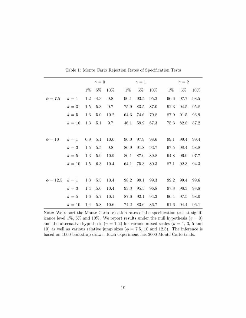
Table 1: Monte Carlo Rejection Rates of Specification Tests

γ = 0 γ = 1 γ = 2

1% 5% 10% 1% 5% 10% 1% 5% 10%

φ = 7.5 k = 1 1.2 4.3 9.8 90.1 93.5 95.2 96.6 97.7 98.5

k = 3 1.5 5.3 9.7 75.9 83.5 87.0 92.3 94.5 95.8

k = 5 1.3 5.0 10.2 64.3 74.6 79.8 87.9 91.5 93.9

k = 10 1.3 5.1 9.7 46.1 59.9 67.3 75.3 82.8 87.2

φ = 10 k = 1 0.9 5.1 10.0 96.0 97.9 98.6 99.1 99.4 99.4

k = 3 1.5 5.5 9.8 86.9 91.8 93.7 97.5 98.4 98.8

k = 5 1.3 5.9 10.9 80.1 87.0 89.8 94.8 96.9 97.7

k = 10 1.5 6.3 10.4 64.1 75.3 80.3 87.1 92.3 94.3

φ = 12.5 k = 1 1.3 5.5 10.4 98.2 99.1 99.3 99.2 99.4 99.6

k = 3 1.4 5.6 10.4 93.3 95.5 96.8 97.8 98.3 98.8

k = 5 1.6 5.7 10.1 87.6 92.1 94.3 96.4 97.5 98.0

k = 10 1.4 5.8 10.6 74.2 83.6 86.7 91.6 94.4 96.1

Note: We report the Monte Carlo rejection rates of the specification test at signif-icance level 1%, 5% and 10%. We report results under the null hypothesis (γ = 0)and the alternative hypothesis (γ = 1, 2) for various mixed scales (k = 1, 3, 5 and10) as well as various relative jump sizes (φ = 7.5, 10 and 12.5). The inference isbased on 1000 bootstrap draws. Each experiment has 2000 Monte Carlo trials.

19

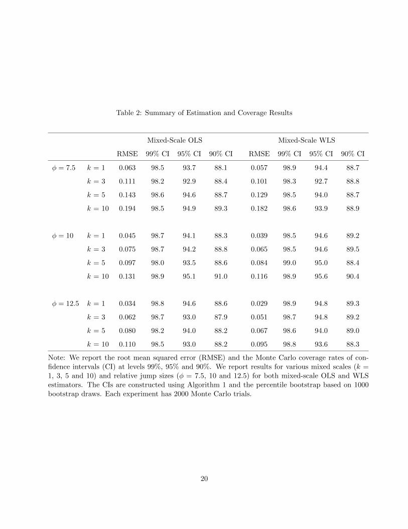
Table 2: Summary of Estimation and Coverage Results

Mixed-Scale OLS Mixed-Scale WLS

RMSE 99% CI 95% CI 90% CI RMSE 99% CI 95% CI 90% CI

φ = 7.5 k = 1 0.063 98.5 93.7 88.1 0.057 98.9 94.4 88.7

k = 3 0.111 98.2 92.9 88.4 0.101 98.3 92.7 88.8

k = 5 0.143 98.6 94.6 88.7 0.129 98.5 94.0 88.7

k = 10 0.194 98.5 94.9 89.3 0.182 98.6 93.9 88.9

φ = 10 k = 1 0.045 98.7 94.1 88.3 0.039 98.5 94.6 89.2

k = 3 0.075 98.7 94.2 88.8 0.065 98.5 94.6 89.5

k = 5 0.097 98.0 93.5 88.6 0.084 99.0 95.0 88.4

k = 10 0.131 98.9 95.1 91.0 0.116 98.9 95.6 90.4

φ = 12.5 k = 1 0.034 98.8 94.6 88.6 0.029 98.9 94.8 89.3

k = 3 0.062 98.7 93.0 87.9 0.051 98.7 94.8 89.2

k = 5 0.080 98.2 94.0 88.2 0.067 98.6 94.0 89.0

k = 10 0.110 98.5 93.0 88.2 0.095 98.8 93.6 88.3

Note: We report the root mean squared error (RMSE) and the Monte Carlo coverage rates of con-fidence intervals (CI) at levels 99%, 95% and 90%. We report results for various mixed scales (k =1, 3, 5 and 10) and relative jump sizes (φ = 7.5, 10 and 12.5) for both mixed-scale OLS and WLSestimators. The CIs are constructed using Algorithm 1 and the percentile bootstrap based on 1000bootstrap draws. Each experiment has 2000 Monte Carlo trials.

20

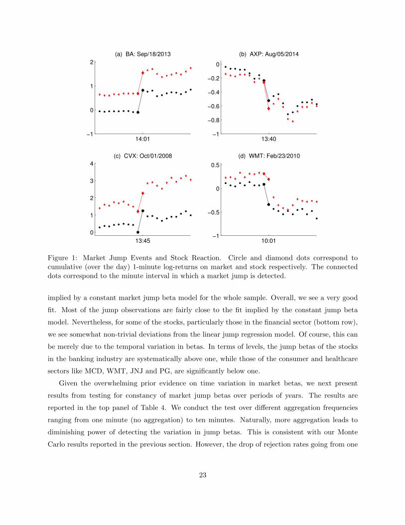
jumps in our sample (two positive and two negative). On Figure 1, we plot the prices of the market

and a set of selected stocks before and after the market jump event. The top left panel shows the

behavior around the market jump on September 18, 2013 which was associated with the (positive)

surprise by the Fed of not tapering its QE programs. In this case, both the market and the BA stock

reacted within the same minute and fully adjusted to their new higher levels. A similar example,

but in the opposite direction, is illustrated on the top right panel of the figure. This panel plots

the market and AXP prices around the market jump on August 5, 2014. There were growing fears

on this day associated with the impact of geopolitical risks on the economy along with concerns

among investors that the Fed might raise interest rates sooner than expected in the wake of signs

that the economy is gaining strength. In this example, like the previous one, both the market and

the stock adjust to their lower level within the minute. Our third example of a market jump is of

October 1, 2008 in the midst of the recent financial crisis. In this case, the CVX stock appeared

to take more than one minute to fully incorporate the positive market jump, a seemingly delayed

reaction which could be driven by market microstructure issues (e.g., stale limit orders). Another

example of this type is the reaction of the WMT stock to the market jump on February 23, 2010

which is displayed on the bottom right panel of Figure 1. This market jump was associated with

a surprisingly weak consumer confidence index reflecting the pessimism among investors for the

strength of the economic recovery. While the market reacted within the minute of the release of

the negative consumer confidence data, the WMT stock took at least 2 minutes to fully incorporate

the bad news.

Overall, the above four examples suggest that, in general, the stocks in our sample react quickly

to the news triggering the market jumps. However, in some instances market microstructure related

issues can confound the reaction of stocks to the market jumps. These issues, however, seem to be

fairly short-lived. To verify that this is indeed the case, in Table 3, we report the jump beta estimates

for all the stocks in the sample using aggregation of 3 and 5 minutes for the beta estimation (and

using the whole sample). In the absence of confounding market microstructure effects, the two beta

estimates should not be statistically different from each other. The results of the table show that

this is largely the case. Indeed, the two beta estimates are fairly close with the median difference

between the 5-minute and 3-minute estimates being only 0.01. The largest difference of 0.14 in our

data set is for the DD stock, and this difference is only marginally statistically significant. Given

this evidence, for the results that follow we will focus attention on the beta estimates based on

three minute aggregation of returns following the market jump.

On Figure 2, we present scatter plots of stock jumps versus market jumps along with the fit

21

Table 3: Full sample WLS beta estimates

Ticker β 95% CI β 95% CI

k = 3 k = 5

AXP 1.15 [1.08; 1.20] 1.17 [1.09; 1.22]

BA 0.99 [0.92; 1.03] 1.02 [0.94; 1.07]

BAC 1.36 [1.27; 1.43] 1.36 [1.25; 1.44]

CAT 1.06 [0.99; 1.11] 1.08 [1.00; 1.13]

CSCO 0.84 [0.77; 0.90] 0.89 [0.82; 0.97]

CVX 0.99 [0.94; 1.03] 0.98 [0.92; 1.02]

DD 1.09 [1.03; 1.14] 1.23 [1.15; 1.27]

DIS 0.97 [0.92; 1.01] 0.98 [0.91; 1.02]

GE 1.16 [1.09; 1.21] 1.17 [1.08; 1.23]

GS 1.20 [1.12; 1.25] 1.21 [1.11; 1.27]

HD 1.05 [0.98; 1.09] 1.07 [0.99; 1.12]

IBM 0.81 [0.76; 0.84] 0.81 [0.75; 0.84]

INTC 0.88 [0.81; 0.94] 0.93 [0.85; 0.99]

JNJ 0.67 [0.62; 0.70] 0.67 [0.62; 0.70]

JPM 1.31 [1.24; 1.37] 1.29 [1.20; 1.34]

KO 0.70 [0.65; 0.74] 0.66 [0.60; 0.70]

MCD 0.51 [0.47; 0.54] 0.50 [0.46; 0.54]

MMM 1.00 [0.95; 1.03] 1.04 [0.97; 1.07]

MRK 0.94 [0.87; 0.97] 0.91 [0.84; 0.95]

MSFT 0.81 [0.75; 0.85] 0.81 [0.75; 0.87]

NKE 0.78 [0.72; 0.83] 0.82 [0.75; 0.87]

PFE 0.87 [0.80; 0.92] 0.88 [0.80; 0.94]

PG 0.68 [0.63; 0.71] 0.65 [0.59; 0.68]

T 0.84 [0.78; 0.88] 0.82 [0.75; 0.86]

TRV 0.94 [0.88; 0.97] 0.86 [0.79; 0.90]

UNH 0.86 [0.80; 0.91] 0.92 [0.84; 0.97]

UTX 1.02 [0.96; 1.05] 1.04 [0.97; 1.08]

VZ 0.72 [0.67; 0.76] 0.71 [0.65; 0.76]

WMT 0.64 [0.59; 0.67] 0.62 [0.57; 0.66]

XOM 0.98 [0.93; 1.02] 0.97 [0.91; 1.01]

Note: We report the efficient k-mixed-scale (k = 3 or 5) WLS estimates and their 95% confidence intervals(CI) of the 30 Dow stocks over the full sample. The CIs are from the percentile bootstrap using 1000 draws.

22

14:01−1

0

1

2

(a) BA: Sep/18/2013

13:40−1

−0.8

−0.6

−0.4

−0.2

0

(b) AXP: Aug/05/2014

13:45

0

1

2

3

4

(c) CVX: Oct/01/2008

10:01−1

−0.5

0

0.5

(d) WMT: Feb/23/2010

Figure 1: Market Jump Events and Stock Reaction. Circle and diamond dots correspond tocumulative (over the day) 1-minute log-returns on market and stock respectively. The connecteddots correspond to the minute interval in which a market jump is detected.

implied by a constant market jump beta model for the whole sample. Overall, we see a very good

fit. Most of the jump observations are fairly close to the fit implied by the constant jump beta

model. Nevertheless, for some of the stocks, particularly those in the financial sector (bottom row),

we see somewhat non-trivial deviations from the linear jump regression model. Of course, this can

be merely due to the temporal variation in betas. In terms of levels, the jump betas of the stocks

in the banking industry are systematically above one, while those of the consumer and healthcare

sectors like MCD, WMT, JNJ and PG, are significantly below one.

Given the overwhelming prior evidence on time variation in market betas, we next present

results from testing for constancy of market jump betas over periods of years. The results are

reported in the top panel of Table 4. We conduct the test over different aggregation frequencies

ranging from one minute (no aggregation) to ten minutes. Naturally, more aggregation leads to

diminishing power of detecting the variation in jump betas. This is consistent with our Monte

Carlo results reported in the previous section. However, the drop of rejection rates going from one

23

−101

BA CAT CSCO CVX DD

−101

DIS GE HD IBM INTC

−101

JNJ KO MCD MMM MRK

−101

MSFT NKE PFE PG T

−101

UNH UTX VZ WMT XOM

−1 0 1

−202 AXP

−1 0 1

BAC

−1 0 1

GS

−1 0 1

JPM

−1 0 1

TRV

Figure 2: Scatter of Stock versus Market Returns at Market Jump Times of the Full Sample.

24

Table 4: Specification testing results for 30 DJIA stocks

2007 2008 2009 2010 2011 2012 2013 2014

Cross-Sectional Rejection Rate

k = 1 0.80 0.77 0.77 0.50 0.50 0.93 0.70 0.77

k = 3 0.50 0.43 0.07 0.17 0.10 0.40 0.33 0.17

k = 5 0.27 0.03 0.00 0.10 0.17 0.40 0.10 0.10

k = 10 0.17 0.10 0.10 0.00 0.00 0.17 0.07 0.03

Cross-Sectional Median of R2

k = 1 0.90 0.90 0.93 0.93 0.97 0.90 0.96 0.91

k = 3 0.86 0.80 0.87 0.92 0.95 0.88 0.95 0.86

k = 5 0.83 0.75 0.87 0.93 0.91 0.88 0.97 0.85

k = 10 0.82 0.81 0.93 0.86 0.87 0.82 0.97 0.81

Note: On the top panel, we report the cross-sectional rejection rate ofthe specification test at 1% significance level for the k-mixed samplesyear-by-year. On the bottom panel, we report the cross-sectionalmedian of the R2s of the 30 stocks for the k-mixed samples.

to three minutes evident from Table 4 is too big to be solely explained by the statistical effect of

losing power when aggregating returns for the jump beta estimation. Instead, the relatively high

rejection rates of the test for one minute aggregation are likely due to market microstructure effects

like the ones illustrated on the bottom panels of Figure 1. At the three minute aggregation level,

the rejection rates of the test are relatively low except for years 2007, 2008 and 2013. Some of

these rejections can be still due to microstructure issues. However, some of the rejections probably

reflect genuine variation of market jump betas, particularly during the period of the recent global

financial crisis.

To further gauge the performance of the year-by-year linear jump regression model, the second

panel of Table 4 reports the R2 of the model fit at the market jump events. As seen from the table,

the R2 numbers are generally very high. For example, the time series average of R2 at one- and

25

three-minute aggregation are 0.93 and 0.89 respectively. As expected from theory, when increasing

aggregation from one minute to ten minutes, the R2 drops because the volatility of the diffusive

aggregated increments around the jumps increases. Nevertheless, we see that with the exception

of year 2008, the loss of R2 going from one-minute to three-minute aggregation is quite moderate.

Comparing the two panels of Table 4, we notice that there is no direct correspondence between the

rejection rates and the magnitude of the R2 of the linear jump regression. For example, focusing

at the three-minute aggregation results, we can see that year 2007 is associated with the highest

rejection rate of the linear jump regression model and yet has relatively high R2. On the other

hand, year 2008 is associated with high rejection rate and is the lowest in the sample R2 (using

again the three-minute aggregation results). This difference can be explained with the different

magnitude of the volatility around the jump event: it is relatively higher in 2008 than in 2007 and,

as a result, the inference in the latter is sharper than the former.

To better assess the time variation in market jump betas, we plot next their time series (using

yearly estimation intervals) on Figure 3. There are some clearly distinguishable time-series patterns

evident from the figure. For example, the market jump betas of stocks in the financial sector, such

as AXP, BAC and JPM, increase in the first two years in our sample and gradually decrease

afterwards. On the other hand, stocks such as INTC and WMT exhibit very little time variation.

The analysis so far has been based at the market jump times. We next investigate how stocks

react to other systematic jump events. In particular, we focus attention on jump events in the nine

industries comprising the S&P 500 index (our proxy for the market index) which are not detected

as market jump events. In a market jump model in which the jumps in stocks are of two types,

idiosyncratic and market, aggregate portfolios, such as the nine industry portfolios, should contain

only jumps at the times when the market jump (as the idiosyncratic jumps get diversified away).

However, some systematic jump events can have much bigger impact on a particular industry

sector than on the market as a whole and, hence, the magnitude of an industry jump can be much

bigger than that of the market co-jump. In such instances, given our discrete setting and high

truncation level, we can fail to detect such jump events on the market level but still find them in a

particular industry sector portfolio. Hence, we label jump events in an industry sector, which are

not detected as market jump times, as sector-specific jumps. These jumps have relatively much

bigger importance for the particular sector than for the market.

To study the reaction of stocks to sector-specific jump events, we first associate with each of the

stocks in our analysis the industry sector it belongs to.18 In Table 5 we report the R2 for a linear

18The stocks in our study are all part of the S&P 500 index during the sample period. We, therefore, use theindustry classification that is used to split the stocks in the S&P 500 index into nine industry portfolio ETFs.

26

0

1

2 BA CAT CSCO CVX DD

0

1

2 DIS GE HD IBM INTC

0

1

2 JNJ KO MCD MMM MRK

0

1

2 MSFT NKE PFE PG T

0

1

2 UNH UTX VZ WMT XOM

0

1

2 AXP BAC GS JPM TRV

Figure 3: Time Series of Yearly Jump Betas, 2007–2014. The dots correspond to the yearly WLSbeta estimates and the shaded areas correspond to the associated 95% confidence intervals.

27

Table 5: R2 of the market factor for two types of jumps.

R2 of Market-wide Jumps

AXP 0.81 HD 0.92 NKE 0.84

BA 0.75 IBM 0.84 PFE 0.84

BAC 0.81 INTC 0.87 PG 0.74

CAT 0.77 JNJ 0.73 T 0.87

CSCO 0.82 JPM 0.70 TRV 0.78

CVX 0.90 KO 0.83 UNH 0.71

DD 0.84 MCD 0.72 UTX 0.85

DIS 0.89 MMM 0.81 VZ 0.85

GE 0.84 MRK 0.81 WMT 0.87

GS 0.72 MSFT 0.84 XOM 0.85

R2 of Sector-specific Jumps

AXP 0.45 HD 0.35 NKE 0.39

BA 0.33 IBM 0.22 PFE 0.46

BAC 0.75 INTC 0.48 PG 0.61

CAT 0.46 JNJ 0.50 T 0.53

CSCO 0.72 JPM 0.83 TRV 0.42

CVX 0.29 KO 0.31 UNH 0.21

DD 0.32 MCD 0.68 UTX 0.52

DIS 0.49 MMM 0.62 VZ 0.58

GE 0.46 MRK 0.32 WMT 0.29

GS 0.45 MSFT 0.78 XOM 0.33

28

jump regression model of the stock jump against the market jump at the sector-specific jump events

for each of the stocks based on the whole sample. For comparison we also report the corresponding

R2 for the linear market jump model at the market jump times. The results present a rather mixed

picture for the performance of the linear market jump model at the sector-specific jump events.

For some stocks such as BAC, JPM, MCD and MSFT, the performance of the linear regression

at the sector-specific jump events in terms of R2 is comparable to its performance at the market

jump events. However, for stocks like CVX, IBM, WMT and XOM, the R2 of the regression at the

sector-specific jump times is very low. Some of the loss of fit when comparing the performance of

the linear jump model at market-wide jump events and sector-specific jump events can be due to

the “signal” being smaller, that is, the market jump size at the sector-specific jump events being

smaller in absolute value. This, however, cannot be the sole explanation, since as explained above,

for some of the stocks in our sample the drop in R2 is quite small. Another reason for the worsening

fit at the sector-specific jump events can be due to larger “noise”, i.e., the diffusive volatility around

the sector-specific jump events can be much bigger than around market-wide jump events for some

of the stocks. Yet a third reason can be that the linear market jump model does not hold at the

sector-specific jump events.

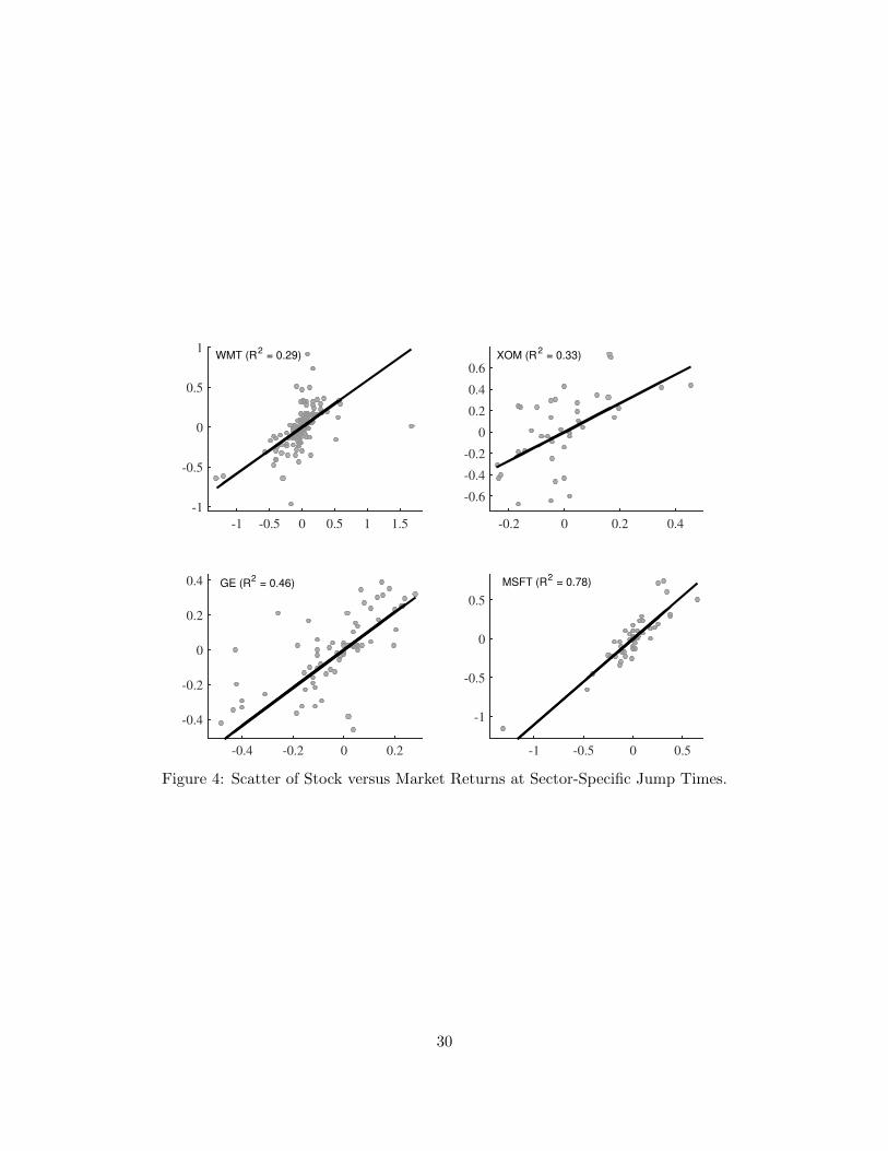
To get further insight in the performance of the linear market jump model at the sector-specific

jump events, we display on Figure 4 scatter plots of the stock jumps against the market jumps at

the sector-specific jump events for four representative (in terms of R2) stocks. As seen from the

figure, the performance of the model for IBM is very good with the observations being very close

to the linear fit. On the other hand, for GE we notice that the jump observations are much more

dispersed around the linear fit. This is suggestive of larger diffusive volatility around the sector-

specific jump events for GE which consequently lowers the R2 of the regression. Similar reasoning

can explain the low R2 for XOM. For this stock, however, we can also notice a few outliers in the

lower left corner of the plot which are indicative of model failure, i.e., that the market jumps cannot

solely explain the XOM jumps at the sector-specific jump events. Finally, the fit for WMT is fairly

poor with no strong association between the stock and market jumps at the sector-specific jump

events. This is in sharp contrast with the performance of the linear jump market model for this

stock at the market jump events.

Overall, we can conclude that for some stocks the linear market jump model continues to work

well at the sector-specific jump events. For many of the stocks, however, this is also associated

with increased diffusive volatility around the sector-specific jump events which makes inference for

the market jump beta at these events much noisier when compared with inference conducted at the

29

-1 -0.5 0 0.5 1 1.5

-1

-0.5

0

0.5

1WMT (R

2 = 0.29)

-0.2 0 0.2 0.4

-0.6

-0.4

-0.2

0

0.2

0.4

0.6

XOM (R2 = 0.33)

-0.4 -0.2 0 0.2

-0.4

-0.2

0

0.2

0.4 GE (R2 = 0.46)

-1 -0.5 0 0.5

-1

-0.5

0

0.5

MSFT (R2 = 0.78)

Figure 4: Scatter of Stock versus Market Returns at Sector-Specific Jump Times.

30

market-wide jump events. Finally, for some of the stocks, the linear market jump model fails to

account for behavior of the stock market jumps at the sector-specific jump events and other factors

are probably needed.

6 Conclusion

We propose a new mixed-scale jump regression framework for studying deterministic dependencies

among jumps in a multivariate setting. A fine time scale is used to identify with high accuracy the

times of large rare jumps in the explanatory variable(s). A coarser scale is then used to conduct

the estimation in order to attenuate the effects of trading friction noise. We derive the asymptotic

properties of an efficient estimator of the jump regression coefficients and a test for its specification.

The limiting distributions of the estimator and the test statistic are non-standard, but a simple

bootstrap method is shown to be valid for feasible inference. We further show that the bootstrap

provides a higher-order refinement that accounts for the sampling variation in spot covariance

estimates which are used to construct the efficient estimator. In a realistically calibrated Monte

Carlo setting, which features leverage effects and price-volatility co-jumps, we report good size and

power properties of the general specification test and good coverage properties of the confidence

intervals.

The empirical application employs a 1-minute panel of Dow stock prices together with the

front-month E-mini S&P 500 stock market index futures over the period 2007–2014. The 1-minute

market index is used to locate jump times, and subsequent 3-minute sampling around the jump

times is used to conduct the jump regression. We find a strong relationship between market jumps

and stock price moves at market jump times. The market jump betas exhibit remarkable temporal

stability and the jump regressions have very high observed R2s. On the other hand, for many of

the stocks in the sample, the relationship between stock and market jumps at sector-specific jump

times is significantly noisier, and temporally more unstable, than the tight relationship seen at

market jump times.

7 Appendix: Proofs

We now prove the theorems in the main text. Throughout this appendix, we use K to denote a

generic positive constant that may change from line to line; we sometimes emphasize the dependence

of this constant on some parameter q by writing Kq. Below, the convergence (ξn,p)p≥1 → (ξp)p≥1, as

n→∞, is understood to be under the product topology. We write w.p.a.1 for “with probability ap-

proaching one.” Recall that (τp)p≥1 are the successive jump times of Z and P = p ≥ 1 : τp ∈ [0, T ].

31

We use i (p) to denote the unique integer such that τp ∈ ((i− 1) ∆n, i∆n].

By a standard localization procedure (see Section 4.4.1 of Jacod and Protter (2012)), we can

respectively strengthen Assumptions 1 and 3 to the following stronger versions without loss of

generality.

Assumption 4. We have Assumption 1. The processes Xt, bt and σt are bounded.

Assumption 5. We have Assumption 3. The processes bt and σt are bounded. Moreover, there

exists some bounded λ-integrable function J such that ‖δ(t, u)‖2 ≤ J (u) for all t ∈ [0, T ] and u ∈ R.

7.1 Proof of Theorem 1

Proof of Theorem 1. By Proposition 1 of Li, Todorov, and Tauchen (2014),

P(Jn = Cn = J ∗n

)→ 1, (7.1)

where Cn is the complement of Cn. Since the jumps of X have finite activity, differences between

distinct indices in Jn can be bounded below by 2kn w.p.a.1 and, hence,cn,i(p)− =

1

kn∆n

kn−1∑j=0

(∆ni(p)−kn+jX)(∆n

i(p)−kn+jX)>1i(p)−kn+j∈Cn,

cn,i(p)+ =1

kn∆n

kn−1∑j=0

(∆ni(p)+k+jX)(∆n

i(p)+k+jX)>1i(p)+k+j∈Cn.

Then, by Theorem 9.3.2 in Jacod and Protter (2012) and ∆ni(p),kZ −→ ∆Zτp , we derive(

cni(p)−, cni(p)+,∆

ni(p),kZ

)P−→(cτp−, cτp ,∆Zτp

).

By (7.1), we see that the following holds w.p.a.1,

βn (w)− β∗

=

∑p∈P

wn,i(p)g(∆ni(p),kZ)g(∆n

i(p),kZ)>

−1∑p∈P

wn,i(p)g(∆ni(p),kZ)εni(p),k

.(7.2)

By Assumption 2, g(·) is continuously differentiable at ∆Zτp almost surely. Then, noting that

∆ni(p),kZ

c = Op(∆1/2n ), we derive

∆−1/2n εni(p),k = ∆−1/2

n

(∆ni(p),kY

c − β∗>(g(∆Zτp + ∆n

i(p),kZc)− g(∆Zτp)

))= ∆−1/2

n

(∆ni(p),kY

c − β∗>∂g(∆Zτp

)∆ni(p),kZ

c)

+ op(1). (7.3)

32

By a straightforward adaptation of Proposition 4.4.10 of Jacod and Protter (2012), we have

∆−1/2n

(∆ni(p),kX

c)p≥1

L-s−→(√

κpστp−ξp− +√k − κpστpξp+

)p≥1

. (7.4)

By (7.3) and (7.4),

∆−1/2n

(εni(p),k

)p≥1

L-s−→ (ςp)p≥1 . (7.5)

From (7.2) and (7.5), it is easy to see that βnP−→ β∗. Hence, wn,i(p)

P−→ wp for each p ≥ 1. From

here, as well as (7.2) and (7.5), we derive

∆−1/2n

(βn (w)− β∗

)L-s−→ Ξ (w)−1 Λ (w)

as asserted. Q.E.D.

7.2 Proof of Theorem 2

Proof of Theorem 2. By Theorem 13.3.3 in Jacod and Protter (2012), we have(k1/2n (cn,i(p)− − cτp−), k1/2

n (cn,i(p)+ − cτp))p≥1

L-s−→ (ζp−, ζp+)p≥1 . (7.6)

This convergence indeed holds jointly with (7.5) because ∆ni,kX

c and (cn,i−, cn,i+) involve non-

overlapping returns. Recall that w(·) is the first differential of w(·), that is, as(c′−, c

′+, z

′, b′)→ 0,

w(c− + c′−, c+ + c′+, z + z′, b+ b′

)− w (c−, c+, z, b)

= w(c−, c+, z, b; c

′−, c′+, z

′, b′)

+ o(∥∥c′−∥∥+

∥∥c′+∥∥+∥∥z′∥∥+

∥∥b′∥∥) .Recall that wp ≡ w

(cτp−, cτp+,∆Zτp , β

∗; ζp−, ζp+, 0, 0). By the delta method, we derive from (7.5),

(7.6), ∆ni(p),kZ = ∆Zτp +Op(∆

1/2n ) and βn = β∗ +Op(∆

1/2n ) that(

k1/2n

(wn,i(p) − wp

),∆−1/2

n εni(p),k

)p≥1

L-s−→ (wp, ςp)p≥1 . (7.7)

We now note that, w.p.a.1,

∆−1/2n

(βn (w)− β∗

)=

∑p∈P

wn,i(p)g(∆ni(p),kZ)g(∆n

i(p),kZ)>

−1∑p∈P

wn,i(p)g(∆ni(p),kZ)∆−1/2

n εni(p),k

=

Ξ (w) +∑p∈P

(wn,i(p) − wp

)g(∆Zτp

)g(∆Zτp

)>+ op(k

−1/2n )

−1

×

∑p∈P

wpg(∆Zτp

)∆−1/2n εni(p),k +

∑p∈P

(wn,i(p) − wp

)g(∆Zτp

)∆−1/2n εni(p),k + op(k

−1/2n )

= Ln (w) + k−1/2

n Hn (w) + op(k−1/2n ),

33

where

Ln (w) ≡ Ξ (w)−1∑p∈P

wpg(∆Zτp

)∆−1/2n εni(p),k,

Hn (w) ≡ Ξ (w)−1∑p∈P

k1/2n

(wn,i(p) − wp

)g(∆Zτp

)∆−1/2n εni(p),k

−Ξ (w)−1

∑p∈P

k1/2n

(wn,i(p) − wp

)g(∆Zτp

)g(∆Zτp

)>Ξ (w)−1

×

∑p∈P

wpg(∆Zτp

)∆−1/2n εni(p),k

.

From (7.7), we have (Ln (w) ,Hn (w))L-s−→ (L (w) ,H (w)) as asserted. Q.E.D.

7.3 Proof of Theorem 3

Proof of Theorem 3. We consider the following set of sample paths

Ωn ≡ Jn = Cn = J ∗n ∩ |i− j| > 2kn for any i, j ∈ Jn with i 6= j .

From (7.1), it is easy to see that P (Ωn) → 1. Hence, we can restrict the calculation below on the

sample paths in Ωn without loss of generality.

Since cn,i(p)± = Op(1), E[‖∆n

i(p),kX∗c‖2

∣∣∣F] = Op(∆n),

E[‖g(∆n

i(p),kZ∗)− g(∆n

i(p),kZ)‖2∣∣∣F] = Op(∆n).

(7.8)

Since βn − βn (w) = Op(∆1/2n ) and kn∆n → 0, we further have

k1/2n

(∆ni(p),kY

∗ − β>n g(∆ni(p),kZ

∗))

= op(1). (7.9)

Note that, w.p.a.1,

k1/2n

(β∗n − βn

)=

∑p∈P

g(∆ni(p),kZ

∗)g(∆ni(p),kZ

∗)>

−1

×

∑p∈P

g(∆ni(p),kZ

∗)k1/2n

(∆ni(p),kY

∗ − β>n g(∆ni(p),kZ

∗)) .

From (7.9), we deduce

k1/2n

(β∗n − βn

)= op(1). (7.10)

34

Next, we observe from (3.9) that c∗n,i(p)± − cn,i(p)± are averages of F-conditionally independent

mean-zero variables with stochastically bounded fourth F-conditional moments. We further note

that

E[(c∗jkn,i(p)± − c

jkn,i(p)±

)(c∗lmn,i(p)± − c

lmn,i(p)±

)∣∣∣F] =1

kn

(cjln,i(p)±c

kmn,i(p)± + cjmn,i(p)±c

kln,i(p)±

),

E[(c∗jkn,i(p)± − c

jkn,i(p)±

)(c∗lmn,i(p)∓ − c

lmn,i(p)∓

)∣∣∣F] = 0.

Upon using a subsequence characterization of convergence in probability and applying Lindeberg’s

central limit theorem under the F-conditional probability, we derive

k1/2n

(c∗n,i(p)− − cn,i(p)−, c

∗n,i(p)+ − cn,i(p)+

)p≥1

L|F−→ (ζp−, ζp+)p≥1 . (7.11)

By (7.8), (7.10) and (7.11), we use the delta method to deduce

k1/2n

(w∗n,i(p) − wn,i(p)

)p≥1

L|F−→ (wp)p≥1 . (7.12)

We now set

εn∗i,k = ∆ni,kY

∗c − βn (w)>(g(∆ni,kZ

∗)− g (∆ni,kZ

)).

Recall the F-conditional distribution of ∆ni,kX

∗c from Algorithm 1. Since βn (w)P−→ β∗ and

∂g(∆ni(p),kZ)

P−→ ∂g(∆Zτp

), we further deduce

∆−1/2n

(εn∗i(p),k

)p≥1

L|F−→ (ςp)p≥1 . (7.13)

Note that, in restriction to Ωn, c∗n,i(p)± and εn∗i(p),k are F-conditionally independent because they do

not involve overlapping increments of W ∗. Hence, (7.12) and (7.13) hold jointly, yielding(∆−1/2n εn∗i(p),k, k

1/2n

(w∗n,i(p) − wn,i(p)

))p≥1

L|F−→ (ςp, wp)p≥1 . (7.14)

For notational simplicity, we denote

Ξn ≡∑p∈P

wn,i(p)g(∆ni(p),kZ)g(∆n

i(p),kZ)>,

Ξ∗n ≡∑p∈P

w∗n,i(p)g(∆ni(p),kZ

∗)g(∆ni(p),kZ

∗)>,

Λ∗n ≡ ∆−1/2n

∑p∈P

w∗n,i(p)g(∆ni(p),kZ

∗)εn∗i(p),k.

Note that, w.p.a.1,

∆−1/2n

(β∗n (w)− βn(w)

)= Ξ∗−1

n Λ∗n. (7.15)

35

By w∗n,i(p) = Op(1) and (7.8), we have

Ξ∗n = Ξn +∑p∈P

(w∗n,i(p) − wn,i(p)

)g(∆n

i(p),kZ)g(∆ni(p),kZ)> +Op(∆

1/2n ).

Therefore,

Ξ∗−1n = Ξ−1

n − Ξ−1n Ξ∗nΞ−1

n + op(k−1/2n ), (7.16)

where Ξ∗n ≡∑

p∈P(w∗n,i(p) − wn,i(p))g(∆ni(p),kZ)g(∆n

i(p),kZ)>.

We decompose

Λ∗n =∑p∈P

wn,i(p)g(∆ni(p),kZ

∗)∆−1/2n εn∗i(p),k

+∑p∈P

(w∗n,i(p) − wn,i(p)

)g(∆n

i(p),kZ∗)∆−1/2

n εn∗i(p),k. (7.17)

Note that Ξ∗n and the second term on the right-hand side of (7.17) are both Op(k−1/2n ). Therefore,

from (7.15), (7.16) and (7.17), we obtain the decomposition

∆−1/2n

(β∗n (w)− βn(w)

)= L∗n (w) + k−1/2

n H∗n (w) + op(k−1/2n ),

where

L∗n (w) ≡ Ξ−1n

∑p∈P

wn,i(p)g(∆ni(p),kZ

∗)∆−1/2n εn∗i(p),k,

H∗n (w) ≡ Ξ−1n

∑p∈P

k1/2n

(w∗n,i(p) − wn,i(p)

)g(∆n

i(p),kZ∗)∆−1/2

n εn∗i(p),k

−Ξ−1n Ξ∗nΞ−1

n

∑p∈P

wn,i(p)g(∆ni(p),kZ

∗)∆−1/2n εn∗i(p),k

.

From (7.14), it is easy to deduce (L∗n (w) ,H∗n (w))L|F−→ (L (w) ,H (w)) as asserted. Q.E.D.

7.4 Proof of Theorem 4

Proof of Theorem 4. (a) Since ∆ni(p),kX

P−→ ∆Xτp , it is easy to see from (2.7) that

SSRnP−→∑p∈P

∆Y 2τp −

∑p∈P

g(∆Zτp

)∆Yτp

>

×

∑p∈P

g(∆Zτp

)g(∆Zτp

)>−1∑p∈P

g(∆Zτp

)∆Yτp

.

36

In particular, the second assertion of part (a) holds. It remains to show the first assertion of part

(a). It is easy to see that

SSRn =∑i∈Jn

∆ni,kY

2 −

(∑i∈Jn

∆ni,kY g

(∆ni,kZ

))>

×

(∑i∈Jn

g(∆ni,kZ

)g(∆ni,kZ

)>)−1(∑i∈Jn

∆ni,kY g

(∆ni,kZ

)).

(7.18)

Plug (2.9) into (7.18). After some elementary algebra, we derive

SSRn =∑i∈Jn

(εni,k)2 −(∑

i∈Jn

εni,kg(∆ni,kZ

))>

×

(∑i∈Jn

g(∆ni,kZ

)g(∆ni,kZ

)>)−1(∑i∈Jn

εni,kg(∆ni,kZ

)).

(7.19)

By (2.7), (7.19) holds w.p.a.1 with Jn replaced by J ∗n . By (7.5) and g(∆ni(p),kZ)

P−→ g(∆Zτp

), we

derive the first assertion of part (a).

(b) Similar to (7.18), we have

SSR∗n =∑i∈Jn

∆ni,kY

∗2 −

(∑i∈Jn

∆ni,kY

∗g(∆ni,kZ

∗))>

×

(∑i∈Jn

g(∆ni,kZ

∗) g (∆ni,kZ

∗)>)−1(∑i∈Jn

∆ni,kY

∗g(∆ni,kZ

∗)) .We now set

εn∗i,k ≡ ∆ni,kY

∗ − β>n g(∆ni,kZ

∗) .After some elementary algebra, we can rewrite

SSR∗n =∑i∈Jn

(εn∗i,k)2 −(∑

i∈Jn

εn∗i,kg(∆ni,kZ

∗))>

×

(∑i∈Jn

g(∆ni,kZ

∗) g (∆ni,kZ

∗)>)−1(∑i∈Jn

εn∗i,kg(∆ni,kZ

∗)) . (7.20)

We further observe εn∗i,k = ∆ni,kY

∗c − β>n (g(∆ni,kZ

∗) − g(∆ni,kZ)). It is easy to show that βn

P−→ β.

From the construction of ∆ni,kX

∗c described in Algorithm 1, as well as the fact that cn,i(p)±P−→ cτp±,

we deduce

∆−1/2n

(εn∗i(p),k

)p≥1

L|F−→ (ςp)p≥1 , (7.21)

37

where ςp ≡(1,−β>∂g

(∆Zτp

))(√κpστp−ξp− +

√k − κpστpξp+). By (7.20) and (7.21), we deduce

∆−1n SSR∗n

L|F−→∑p∈P

ς2p −

∑p∈P

g(∆Zτp

)ςp

>

×

∑p∈P

g(∆Zτp

)g(∆Zτp

)>−1∑p∈P

g(∆Zτp

)ςp

.

(7.22)

In restriction to Ω0, the limiting distribution characterized by (7.22) coincides with the limiting

distribution of ∆−1n SSRn. We further note that, conditionally on F , this limiting distribution is

atomless with positive density on (0,∞). Therefore, the F-conditional (1 − α)-quantile of this

limiting distribution can be consistently estimated by ∆−1n cvαn . From here and part (a) of this

theorem, it readily follows that P (SSRn > cvαn |Ω0)→ α.

In restriction to Ωa, we see from part (a) that the probability limit of SSRn is strictly positive.

Moreover, the sequence ∆−1n cvαn is still tight because of (7.22). The assertion P (SSRn > cvαn |Ωa)→

1 readily follows. Q.E.D.

References

Andersen, T. G., T. Bollerslev, F. X. Diebold, and C. Vega (2003): “Micro Effects of MacroAnnouncements: Real-Time Price Discovery in Foreign Exchange,” The American Economic Review,93(1), 251 – 277.

Andersen, T. G., T. Bollerslev, F. X. Diebold, and G. Wu (2006): “Realized Beta: Persistenceand Predictability.,” in , vol. 20 (Part 2) of Advances in Econometrics: Econometric Analysis of Financialand Economic Time Series, pp. 1–39. Emerald Group Publishing Limited.

Bandi, F., and R. Reno (2015): “Price and Volatility Co-jumps,” Journal of Financial Economics,Forthcoming.

Barndorff-Nielsen, O., P. Hansen, A. Lunde, and N. Shephard (2009): “Realized kernels in prac-tice: trades and quotes,” The Econometrics Journal, 12(3), C1–C32.

Barndorff-Nielsen, O. E., and N. Shephard (2004a): “Econometric Analysis of Realized Covariation:High Frequency Based Covariance, Regression, and Correlation in Financial Economics.,” Econometrica,72(3), 885 – 925.

Barndorff-Nielsen, O. E., and N. Shephard (2004b): “Power and Bipower Variation with StochasticVolatility and Jumps,” Journal of Financial Econometrics, 2, 1–37.

Davison, A. C., and D. V. Hinkley (1997): Bootstrap Methods and their Application, Cambridge Seriesin Statistical and Probabilistic Mathematics. Cambridge University Press.

Dovonon, P., S. Goncalves, and N. Meddahi (2013): “Bootstrapping Realized Multivariate VolatilityMeasures,” Journal of Econometrics, 172(1), 49 – 65.

Dovonon, P., U. Hounyo, S. Goncalves, and N. Meddahi (2014): “Bootstrapping High FrequencyJump Tests,” Discussion paper, Toulouse School of Economics.

38

Gobbi, F., and C. Mancini (2012): “Identifying the Brownian Covariation from the Co-Jumps givenDiscrete Observations,” Econometric Theory, 28, 249–273.

Goncalves, S., and N. Meddahi (2009): “Bootstrapping Realized Volatility,” Econometrica, 77, 283–306.

Hasbrouck, J. (2003): “Intraday Price Formation in U.S. Equity Index Markets,” The Journal of Finance,58(6), 2375–2399.

Hasbrouck, J. (2015): “Securities Trading: Procedures and Principles,” Discussion paper, New YorkUniversity.

Horowitz, J. L. (2001): “The Bootstrap,” in Handbook of Econometrics, vol. 5. Elsevier.

Hounyo, U. (2013): “Bootstrapping Realized Volatility and Realized Beta under a Local GaussianityAssumption,” Discussion paper, University of Oxford.

Jacod, J., and P. Protter (2012): Discretization of Processes. Springer.

Jacod, J., and V. Todorov (2010): “Do Price and Volatility Jump Together?,” Annals of AppliedProbability, 20, 1425–1469.

Kalnina, I. (2013): “Nonparametric Tests of Time Variation in Betas,” Discussion paper, University ofMontreal.

Kyle, A. S. (1985): “Continuous Auctions and Insider Trading,” Econometrica, 53(6), pp. 1315–1335.

Lehmann, E. L., and J. P. Romano (2005): Testing Statistical Hypothesis. Springer.

Li, J., V. Todorov, and G. Tauchen (2014): “Jump Regression,” Discussion paper, Duke Univeristy.

Mancini, C. (2001): “Disentangling the Jumps of the Diffusion in a Geometric Jumping Brownian Motion,”Giornale dell’Istituto Italiano degli Attuari, LXIV, 19–47.

Merton, R. C. (1976): “Option Pricing When Underlying Stock Returns Are Discontinuous.,” Journal ofFinancial Economics, 3(1/2), 125 – 144.

Mykland, P., and L. Zhang (2009): “Inference for Continuous Semimartingales Observed at High Fre-quency,” Econometrica, 77, 1403–1445.

Reiss, M., V. Todorov, and G. Tauchen (2015): “Nonparametric Test for a Constant Beta betweenIto Semimartingales based on High-Frequency Data,” Stochastic Processes and their Applications, 125,2955–2988.

Roll, R. (1987): “R2,” Journal of Finance, 43, 541–566.

Todorov, V., and T. Bollerslev (2010): “Jumps and Betas: A New Framework for Disentangling andEstimating Systematic Risks,” Journal of Econometrics, 157, 220–235.

Todorov, V., and G. Tauchen (2011): “Volatility Jumps,” Journal of Business and Economic Statistics,29, 356–371.

(2012): “The Realized Laplace Transform of Volatility,” Economtrica, 80, 1105–1127.

Zhang, L., P. A. Mykland, and Y. Aıt-Sahalia (2005): “A Tale of Two Time Scales: DeterminingIntegrated Volatility with Noisy High-Frequency Data,” Journal of the American Statistical Association,100, 1394–1411.

39