modeling and verification of early age thermal stress in

Modeling and verification of early age thermal stress in secondlining concrete of NATM tunnels.Chamila Kumara Rankoth, Akira Hosoda Keitai Iwama,Journal of Advanced Concrete Technology, volume ( ), pp.15 2017 213-226

Analysis of Crack Propagation due to Thermal Stress in Concrete Considering Solidified ConstitutiveModelWorapong Srisoros, Hikaru Nakamura Minoru Kunieda, , Yasuaki IshikawaJournal of Advanced Concrete Technology, volume ( ), pp.5 2007 99-112

Multiscale model for creep of shotcrete- from logarithmic-type viscous behavior of CSH at the μm-scaleto macroscopic tunnel analysisChristian Pichler , Roman Lackner Herbert A. Mang,Journal of Advanced Concrete Technology, volume ( ), pp.6 2008 91-110

https://www.jstage.jst.go.jp/article/jact/5/1/5_1_99/_pdf

https://www.jstage.jst.go.jp/article/jact/6/1/6_1_91/_pdf

http://www.editorialmanager.com/jact/default.aspx

http://www.j-act.org/index.html

Journal of Advanced Concrete Technology Vol. 15, 213-226, June 2017 / Copyright © 2017 Japan Concrete Institute 213

Scientific paper

Modeling and Verification of Early Age Thermal Stress in Second Lining Concrete of NATM Tunnels Chamila K. Rankoth1*, Akira Hosoda2 and Keitai Iwama3

Received 5 February 2017, accepted 31 May 2017 doi:10.3151/jact.15.213

Abstract The objective of this research is to establish proper modeling of FEM simulation for early thermal stress in second lin-ing concrete of NATM tunnels. The proposed model was verified by field measurements. Stresses at the crown and at the sides close to the invert of the second lining were investigated using the established FEM model. First, a simulation scheme was proposed considering thermal behaviors in detail and was sufficiently verified using tunnel monitoring data obtained from a previous study. It was observed that accurate modeling was indispensable for the variation of air tem-perature and for thermal properties of waterproofing membrane to obtain dependable temperature simulation results. Second, appropriate modeling for several kinds of joints and important inputs related to early thermal stress such as effective Young’s modulus, autogenous shrinkage development, and setting of hardening time were proposed. Simula-tion results of structural strain and stress were verified by measurement data in a recently constructed tunnel. Slight dif-ference between simulation results and measurement might be partially due to the material model idealizations and due to the structural imperfections in actual structures. From the stress distributions extracted from the simulation results, it was observed that the crown cracks might be non-penetrating cracks and the cracks close to invert might be penetrating cracks.

1. Introduction

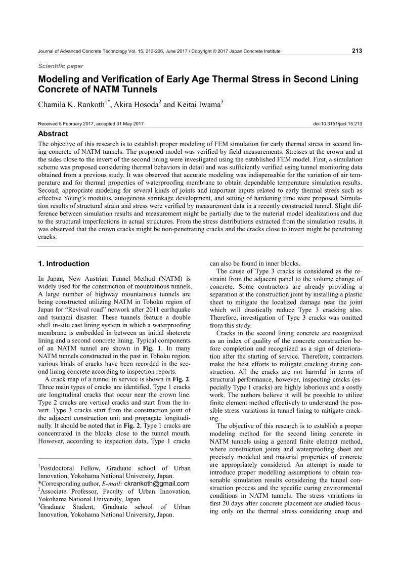
In Japan, New Austrian Tunnel Method (NATM) is widely used for the construction of mountainous tunnels. A large number of highway mountainous tunnels are being constructed utilizing NATM in Tohoku region of Japan for “Revival road” network after 2011 earthquake and tsunami disaster. These tunnels feature a double shell in-situ cast lining system in which a waterproofing membrane is embedded in between an initial shotcrete lining and a second concrete lining. Typical components of an NATM tunnel are shown in Fig. 1. In many NATM tunnels constructed in the past in Tohoku region, various kinds of cracks have been recorded in the sec-ond lining concrete according to inspection reports.

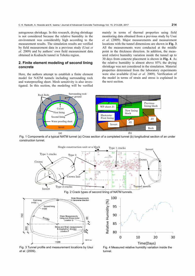
A crack map of a tunnel in service is shown in Fig. 2. Three main types of cracks are identified. Type 1 cracks are longitudinal cracks that occur near the crown line. Type 2 cracks are vertical cracks and start from the in-vert. Type 3 cracks start from the construction joint of the adjacent construction unit and propagate longitudi-nally. It should be noted that in Fig. 2, Type 1 cracks are concentrated in the blocks close to the tunnel mouth. However, according to inspection data, Type 1 cracks

can also be found in inner blocks. The cause of Type 3 cracks is considered as the re-

straint from the adjacent panel to the volume change of concrete. Some contractors are already providing a separation at the construction joint by installing a plastic sheet to mitigate the localized damage near the joint which will drastically reduce Type 3 cracking also. Therefore, investigation of Type 3 cracks was omitted from this study.

Cracks in the second lining concrete are recognized as an index of quality of the concrete construction be-fore completion and recognized as a sign of deteriora-tion after the starting of service. Therefore, contractors make the best efforts to mitigate cracking during con-struction. All the cracks are not harmful in terms of structural performance, however, inspecting cracks (es-pecially Type 1 cracks) are highly laborious and a costly work. The authors believe it will be possible to utilize finite element method effectively to understand the pos-sible stress variations in tunnel lining to mitigate crack-ing.

The objective of this research is to establish a proper modeling method for the second lining concrete in NATM tunnels using a general finite element method, where construction joints and waterproofing sheet are precisely modeled and material properties of concrete are appropriately considered. An attempt is made to introduce proper modelling assumptions to obtain rea-sonable simulation results considering the tunnel con-struction process and the specific curing environmental conditions in NATM tunnels. The stress variations in first 20 days after concrete placement are studied focus-ing only on the thermal stress considering creep and

1Postdoctoral Fellow, Graduate school of Urban Innovation, Yokohama National University, Japan. *Corresponding author, E-mail: [email protected] Professor, Faculty of Urban Innovation, Yokohama National University, Japan. 3Graduate Student, Graduate school of Urban Innovation, Yokohama National University, Japan.

C. K. Rankoth, A. Hosoda and K. Iwama / Journal of Advanced Concrete Technology Vol. 15, 213-226, 2017 214

autogenous shrinkage. In this research, drying shrinkage is not considered because the relative humidity in the environment was considerably high according to the measurement results. The simulation results are verified by field measurement data in a previous study (Usui et al. 2009) and by authors’ own field measurement data obtained in Kodsuchi tunnel in Tohoku region.

2. Finite element modeling of second lining concrete

Here, the authors attempt to establish a finite element model for NATM tunnels including surrounding rock and waterproofing sheet. Mesh sensitivity is also inves-tigated. In this section, the modeling will be verified

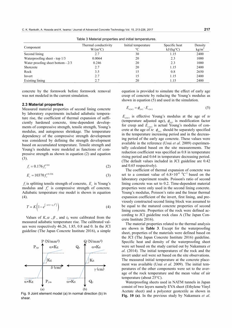
mainly in terms of thermal properties using field monitoring data obtained from a previous study by Usui et al. (2009). Major measurements and measurement locations with the tunnel dimensions are shown in Fig. 3. All the measurements were conducted at the middle point in the thickness direction. In addition, the meas-ured relative humidity variation inside the tunnel up to 30 days from concrete placement is shown in Fig. 4. As the relative humidity is almost above 85% the drying shrinkage was not considered in the simulation. Material properties determined from the laboratory experiments were also available (Usui et al. 2009). Verification of the model in terms of strain and stress is explained in the next section.

Surrounding rock/ ground

Rock Bolts

Second lining

Water proofing sheet

Invert

Crown First lining

Shotcrete-First lining

New lining block

Previous lining block

Rock

WP sheet J1

J3 J2

Invert

(a) (b) Fig. 1 Components of a typical NATM tunnel (a) Cross section of a completed tunnel (b) longitudinal section of an under construction tunnel.

Type 1 cracks

Type 2 cracks

Type 3

Tunnel mouth

Crown

Invert

Crown line

Invert

Crown

Type 1 cracks Single construction unit or a block

Fig. 2 Crack types of second lining of NATM tunnels.

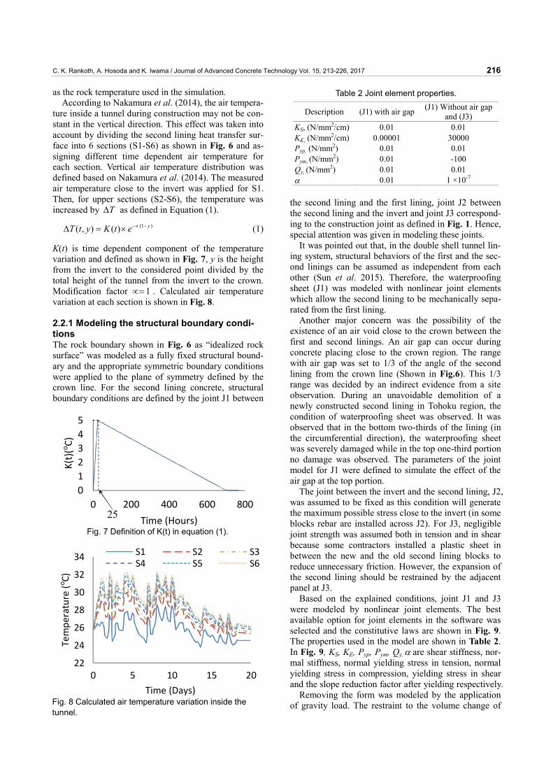
Fig. 3 Tunnel profile and measurement locations by Usui et al. (2009).

80

85

90

95

100

0 10 20 30

Relative Hum

idity

(%)

Time(Days)Fig. 4 Measured relative humidity variation inside the tunnel.


2.1 Simulation software A commercial finite element package (ASTEA-MACS, Version 8.5.3), specially designed for thermal stress analysis of concrete structures was utilized in the study. Thermal analysis is followed by the structural stress analysis. Linear hexahedral isoparametric elements were utilized in both thermal and structural analysis. 2.2 Finite element model and boundary condi-tions A three-dimensional model is essential for studying the stress conditions pertaining to Type 1 and Type 2 cracks. Only a half of the tunnel was modeled considering the symmetry along the crown line. The completed model is shown in Fig. 5 with the heat transfer boundary condi-tions. A detailed cross -section is shown in Fig. 6. The length of the modeled second lining block was 12.2m and the thickness was 0.3 m. The thicknesses of the in-vert, rock layer, and shotcrete were 0.45 m, 2 m, and 0.15 m respectively. The length of the previously con-creted lining was 6.1m. 2.2.1 Modeling the thermal boundary condi-tions Thermal boundary conditions were carefully defined based on actual site conditions and referring past re-search results. The heat transfer surface definition is shown in Fig. 5.

The heat transfer coefficients related to all the sur-faces are shown in Table 1. In the case of second lining surface, the recommended value by the The Japan Con-crete Institute (2016) for both steel formwork surface

and concrete surface after formwork removal is 14 W/m2k-1. However, based on previous studies (Naka-mura et al. 2014; Ohno and Hosoda 2012), it was ob-served that the heat transfer coefficient of the concrete surface can be lower than the recommended value in many cases. Therefore, it was set to 6 W/m2k-1 before formwork removal based on the study by Ohno and Ho-soda (2012). After formwork removal, heat transfer co-efficient was set to 10 W/m2k-1 considering the special environmental conditions inside tunnels where concrete surface is less frequently subjected to moving air due to special curing methods (for example, Fig.18).

Especially in tunnels, the heat transfer coefficient of the formwork surface can be reduced in some cases be-cause concreting is done in a covered environment. Heat transfer coefficient of the invert surface was also set to a lower value considering the fact that this surface is cov-ered by soil at the starting of second lining construction.

The modeled thickness of the rock should be large enough to represent the thermal behavior to an acceptable level and should be small enough not to in-crease analysis time substantially. Furthermore, if a very large soil thickness is used in the modeling, the soil de-formation due to self-weight was found to be generating unusual simulation results in the second lining. The thickness was decided as 2m based on a parametric study and a convection surface was assigned to the back surface of the rock to prevent thermal accumulation in the rock layer. The surface temperature for this heat transfer surface was assigned as 15°C which was same

Table 1 Heat transfer coefficients related to heat transfer surfaces.

Heat Transfer Coefficient (W/m2k-1) Component Before formwork removal After formwork removal

Reference/ Reason

Second lining surface 6 10 Ohno and Hosoda (2012) Invert surface 6 6 covered in soil Existing lining surface 14 14 Surface of the first lining 14 14 Japan Concrete Institute (2016)

Idealized surface of the rock 3.5 3.5 parametric study

S5S6S4

S2S1

Invert

Rock

S3

Shotcrete –First lining

Waterproofing sheet without air gap

Waterproofing sheet with air gap

Second lining

Second lining surface divided to 6 sections S1—S6 – different air temperature assigned

Idealized rock surface

1/3 of lining angle

Fig. 6 Cross section and the components of the model (components are exaggerated).

Invert surface

Existing lining surface

Surface of the first lining (Shotcrete)

Second lining surface

Idealized rock surface

2m

12.2 m

Fig. 5 Established model and the heat transfer surfaces.


as the rock temperature used in the simulation. According to Nakamura et al. (2014), the air tempera-

ture inside a tunnel during construction may not be con-stant in the vertical direction. This effect was taken into account by dividing the second lining heat transfer sur-face into 6 sections (S1-S6) as shown in Fig. 6 and as-signing different time dependent air temperature for each section. Vertical air temperature distribution was defined based on Nakamura et al. (2014). The measured air temperature close to the invert was applied for S1. Then, for upper sections (S2-S6), the temperature was increased by TΔ as defined in Equation (1).

(1 )( , ) ( ) yT t y K t e−∝ −Δ = × (1)

K(t) is time dependent component of the temperature variation and defined as shown in Fig. 7, y is the height from the invert to the considered point divided by the total height of the tunnel from the invert to the crown. Modification factor 1∝= . Calculated air temperature variation at each section is shown in Fig. 8.

2.2.1 Modeling the structural boundary condi-tions The rock boundary shown in Fig. 6 as “idealized rock surface” was modeled as a fully fixed structural bound-ary and the appropriate symmetric boundary conditions were applied to the plane of symmetry defined by the crown line. For the second lining concrete, structural boundary conditions are defined by the joint J1 between

the second lining and the first lining, joint J2 between the second lining and the invert and joint J3 correspond-ing to the construction joint as defined in Fig. 1. Hence, special attention was given in modeling these joints.

It was pointed out that, in the double shell tunnel lin-ing system, structural behaviors of the first and the sec-ond linings can be assumed as independent from each other (Sun et al. 2015). Therefore, the waterproofing sheet (J1) was modeled with nonlinear joint elements which allow the second lining to be mechanically sepa-rated from the first lining.

Another major concern was the possibility of the existence of an air void close to the crown between the first and second linings. An air gap can occur during concrete placing close to the crown region. The range with air gap was set to 1/3 of the angle of the second lining from the crown line (Shown in Fig.6). This 1/3 range was decided by an indirect evidence from a site observation. During an unavoidable demolition of a newly constructed second lining in Tohoku region, the condition of waterproofing sheet was observed. It was observed that in the bottom two-thirds of the lining (in the circumferential direction), the waterproofing sheet was severely damaged while in the top one-third portion no damage was observed. The parameters of the joint model for J1 were defined to simulate the effect of the air gap at the top portion.

The joint between the invert and the second lining, J2, was assumed to be fixed as this condition will generate the maximum possible stress close to the invert (in some blocks rebar are installed across J2). For J3, negligible joint strength was assumed both in tension and in shear because some contractors installed a plastic sheet in between the new and the old second lining blocks to reduce unnecessary friction. However, the expansion of the second lining should be restrained by the adjacent panel at J3.

Based on the explained conditions, joint J1 and J3 were modeled by nonlinear joint elements. The best available option for joint elements in the software was selected and the constitutive laws are shown in Fig. 9. The properties used in the model are shown in Table 2. In Fig. 9, KS, KE, Pyp, Pym, Qy, α are shear stiffness, nor-mal stiffness, normal yielding stress in tension, normal yielding stress in compression, yielding stress in shear and the slope reduction factor after yielding respectively.

Removing the form was modeled by the application of gravity load. The restraint to the volume change of

Table 2 Joint element properties.

Description (J1) with air gap (J1) Without air gap and (J3)

KS, (N/mm2/cm) 0.01 0.01 KE, (N/mm2/cm) 0.00001 30000 Pyp, (N/mm2) 0.01 0.01 Pym, (N/mm2) 0.01 -100 Qy, (N/mm2) 0.01 0.01 α 0.01 1 ×10-7

012345

0 200 400 600 800

Time (Hours)25

K(t)(oC)

Fig. 7 Definition of K(t) in equation (1).

22

24

26

28

30

32

34

0 5 10 15 20

Tempe

rature (oC)

Time (Days)

S1 S2 S3S4 S5 S6

Fig. 8 Calculated air temperature variation inside the tunnel.


concrete by the formwork before formwork removal was not modeled in the current simulation.

2.3 Material properties Measured material properties of second lining concrete by laboratory experiments included adiabatic tempera-ture rise, the coefficient of thermal expansion of suffi-ciently hardened concrete, time-dependent develop-ments of compressive strength, tensile strength, Young’s modulus, and autogenous shrinkage. The temperature dependency of the compressive strength development was considered by defining the strength development based on accumulated temperature. Tensile strength and Young’s modulus were modeled as functions of com-pressive strength as shown in equation (2) and equation (3).

0.80.176t cf f ′= (2)

0.32610370c cE f ′= (3)

tf is splitting tensile strength of concrete, cE is Young’s modulus and cf ′ is compressive strength of concrete. Adiabatic temperature rise model is shown in equation (4).

( )( )0( )1 t tT K eβα− −

= − (4)

Values of K, α , β , and t0 were calibrated from the measured adiabatic temperature rise. The calibrated val-ues were respectively 46.26, 1.85, 0.8 and 0. In the JCI guideline (The Japan Concrete Institute 2016), a simple

equation is provided to simulate the effect of early age creep of concrete by reducing the Young’s modulus as shown in equation (5) and used in the simulation.

( ) ( ) ( )e te te c teE Eφ= ⋅ (5)

( )e teE is effective Young’s modulus at the age of te (temperature adjusted age), ( )teφ is modification factor for creep and ( )c teE is actual Young’s modulus of con-crete at the age of te. ( )teφ should be separately specified in the temperature increasing period and in the decreas-ing period of the early age concrete. These values were available in the reference (Usui et al. 2009) experimen-tally calculated based on the site measurements. The reduction coefficient was specified as 0.8 in temperature rising period and 0.64 in temperature decreasing period. (The default values included in JCI guideline are 0.42 and 0.65 respectively).

The coefficient of thermal expansion of concrete was set to a constant value of 6.8×10-6 oC-1 based on the laboratory experiment results. Poisson's ratio of second lining concrete was set to 0.2. Time-dependent material properties were only used in the second lining concrete. Young’s modulus, Poisson’s ratio and the linear thermal expansion coefficient of the invert, first lining, and pre-viously constructed second lining block was assumed to be equal to the matured concrete properties of second lining concrete. Properties of the rock were defined ac-cording to JCI guideline rock class A (The Japan Con-crete Institute 2016).

The material properties related to the thermal analysis are shown in Table 3. Except for the waterproofing sheet, properties of the materials were defined based on the JCI (The Japan Concrete Institute 2016) guideline. Specific heat and density of the waterproofing sheet were set based on the study carried out by Nakamura et al. (2014). The initial temperatures of the rock and the invert under soil were set based on the site observations. The measured initial temperature at the concrete place-ment was available (Usui et al. 2009). The initial tem-peratures of the other components were set to the aver-age of the rock temperature and the mean value of air temperature (about 25°C).

Waterproofing sheets used in NATM tunnels in Japan consist of two layers namely EVA sheet (Ethylene Vinyl Acetate sheet) and a polyester geotextile as shown in Fig. 10 (a). In the previous study by Nakamura et al.

Table 3 Material properties and initial temperatures.

Component Thermal conductivity W/(m°C)

Initial temperature °C

Specific heat kJ/(kg°C)

Density kg/m3

Second lining 2.7 30 1.15 2400 Waterproofing sheet - top 1/3 0.0064 20 2.3 1000 Water proofing sheet bottom - 2/3 0.246 20 2.3 1000 Shotcrete 2.7 20 1.15 2400 Rock 3.5 15 0.8 2650 Invert 2.7 15 1.15 2400 Existing lining 2.7 20 1.15 2400

KE

α×KE Pyp

Pym α×KE

P (N/mm2)

δ (cm)

KS

α×KSQy

-Qy α×KS

Q (N/mm2)

γ (cm)

(a) (b) Fig. 9 Joint element model (a) In normal direction (b) In shear.


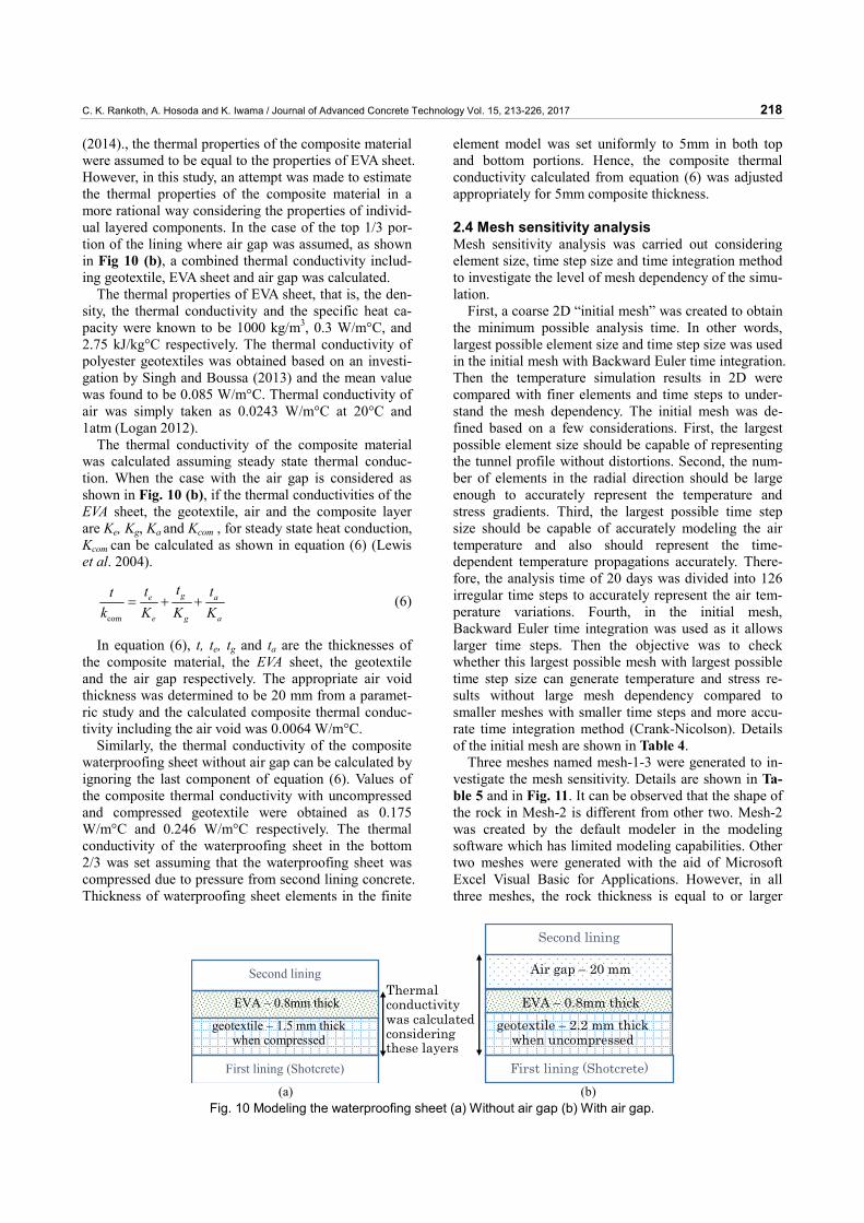
(2014)., the thermal properties of the composite material were assumed to be equal to the properties of EVA sheet. However, in this study, an attempt was made to estimate the thermal properties of the composite material in a more rational way considering the properties of individ-ual layered components. In the case of the top 1/3 por-tion of the lining where air gap was assumed, as shown in Fig 10 (b), a combined thermal conductivity includ-ing geotextile, EVA sheet and air gap was calculated.

The thermal properties of EVA sheet, that is, the den-sity, the thermal conductivity and the specific heat ca-pacity were known to be 1000 kg/m3, 0.3 W/m°C, and 2.75 kJ/kg°C respectively. The thermal conductivity of polyester geotextiles was obtained based on an investi-gation by Singh and Boussa (2013) and the mean value was found to be 0.085 W/m°C. Thermal conductivity of air was simply taken as 0.0243 W/m°C at 20°C and 1atm (Logan 2012).

The thermal conductivity of the composite material was calculated assuming steady state thermal conduc-tion. When the case with the air gap is considered as shown in Fig. 10 (b), if the thermal conductivities of the EVA sheet, the geotextile, air and the composite layer are Ke, Kg, Ka and Kcom , for steady state heat conduction, Kcom can be calculated as shown in equation (6) (Lewis et al. 2004).

com

ge a

e g a

tt ttk K K K

= + + (6)

In equation (6), t, te, tg and ta are the thicknesses of the composite material, the EVA sheet, the geotextile and the air gap respectively. The appropriate air void thickness was determined to be 20 mm from a paramet-ric study and the calculated composite thermal conduc-tivity including the air void was 0.0064 W/m°C.

Similarly, the thermal conductivity of the composite waterproofing sheet without air gap can be calculated by ignoring the last component of equation (6). Values of the composite thermal conductivity with uncompressed and compressed geotextile were obtained as 0.175 W/m°C and 0.246 W/m°C respectively. The thermal conductivity of the waterproofing sheet in the bottom 2/3 was set assuming that the waterproofing sheet was compressed due to pressure from second lining concrete. Thickness of waterproofing sheet elements in the finite

element model was set uniformly to 5mm in both top and bottom portions. Hence, the composite thermal conductivity calculated from equation (6) was adjusted appropriately for 5mm composite thickness.

2.4 Mesh sensitivity analysis Mesh sensitivity analysis was carried out considering element size, time step size and time integration method to investigate the level of mesh dependency of the simu-lation.

First, a coarse 2D “initial mesh” was created to obtain the minimum possible analysis time. In other words, largest possible element size and time step size was used in the initial mesh with Backward Euler time integration. Then the temperature simulation results in 2D were compared with finer elements and time steps to under-stand the mesh dependency. The initial mesh was de-fined based on a few considerations. First, the largest possible element size should be capable of representing the tunnel profile without distortions. Second, the num-ber of elements in the radial direction should be large enough to accurately represent the temperature and stress gradients. Third, the largest possible time step size should be capable of accurately modeling the air temperature and also should represent the time-dependent temperature propagations accurately. There-fore, the analysis time of 20 days was divided into 126 irregular time steps to accurately represent the air tem-perature variations. Fourth, in the initial mesh, Backward Euler time integration was used as it allows larger time steps. Then the objective was to check whether this largest possible mesh with largest possible time step size can generate temperature and stress re-sults without large mesh dependency compared to smaller meshes with smaller time steps and more accu-rate time integration method (Crank-Nicolson). Details of the initial mesh are shown in Table 4.

Three meshes named mesh-1-3 were generated to in-vestigate the mesh sensitivity. Details are shown in Ta-ble 5 and in Fig. 11. It can be observed that the shape of the rock in Mesh-2 is different from other two. Mesh-2 was created by the default modeler in the modeling software which has limited modeling capabilities. Other two meshes were generated with the aid of Microsoft Excel Visual Basic for Applications. However, in all three meshes, the rock thickness is equal to or larger

geotextile – 1.5 mm thick when compressed

EVA – 0.8mm thick

First lining (Shotcrete)

Second lining Thermal conductivity was calculated considering these layers

geotextile – 2.2 mm thick when uncompressed

EVA – 0.8mm thick

First lining (Shotcrete)

Second lining

Air gap – 20 mm

(a) (b)

Fig. 10 Modeling the waterproofing sheet (a) Without air gap (b) With air gap.


than 2m. Hence, the different rock shapes have little effect on the simulation results.

Considering the thermal propagation, time step size depends on the minim dimension of the smallest ele-ment. Time step sizes considering changed element sizes were calculated using equation (7) (Research Cen-ter of Computational Mechanics. Inc. 2015)

2( 1)4

Ct ρλ

ΔΔ = (7)

tΔ is the required minimum time step size in hours, lΔ is the element smallest dimension in governing tem-

perature propagation direction in meters, ρ is the mate-rial density in kg/m3, C is the specific heat capacity of

the material in kcal/kg°C, and λ is the thermal conduc-tivity of the material in kcal/mh°C. It was found that the governing elements considering the thermal propagation are elements in the bottom section of the waterproofing sheet which required the time step size to be as small as 0.016 hours according to equation (7). Therefore, the analysis time of 20 days was divided in to uniform 32000 steps for Mesh-1 and Mesh-2.

Then, the mesh sensitivity analysis was carried out using three-dimensional models to investigate the mesh size in the longitudinal direction. Again, three models were created as 3DMesh-1-3 and the details are shown Fig. 12. In all three meshes vertical element size was approximately 200 mm. However, the longitudinal ele-ment size of the 3DMesh-1 (created using default mod-eler in ASTEA-MACS) had a maximum length of about

Table 4 Details of the Initial mesh.

Component Approximate minimum size – mm (Radial × Circumferential)

Number of Elements- (Radial × Circumferential)

Second lining 50 × 200 288-(6×48) Waterproofing sheet 5 × 200 (Joint element) 48-(1×48) Shotcrete 50 × 200 144-(3×48) Invert 50 × 200 160-(10×16) Rock 225 × 200 288-(4×64) Total number of elements 928

Table 5 Purposes of different types of meshes.

Mesh Purpose Features Mesh - 1 Investigate the effect of the mesh density in rock region Rock with finer elements. Maximum thickness in radial

direction was 100mm Mesh - 2 Effect of mesh size in the second lining Second lining element size was reduced to 16mm × 80 mm. Mesh - 3 Effect of aspect ratio in 2D Second lining element size 50 mm x 50 mm

Mesh -1 Mesh -2 Mesh -3

Aspect ratio of Second lining kept as 1

Fine mesh in Second lining

Fine mesh in rock in radial direction

(a) (b) (c)

Fig. 11 Three types of meshes used for mesh sensitivity analysis.

Element size is changing in longitudinal direction

Element size is 200 mm in longitudinal direction

50mm elements where air temperature changes

(a) (b) (c) Fig. 12.Three dimensional meshes used in the mesh sensitivity analysis. (a) 3DMesh-1 (b) 3DMesh-2 (c) 3DMesh-3.


660 mm (aspect ratio 3.3) other two meshes had a uni-form longitudinal element size of 200 mm. In 3DMesh-3, smaller elements were created where air temperature changed as shown in Fig. 12.

Comparison of the simulated time dependent varia-tions of four selected 2D models is shown in Fig. 13, and the comparison of the estimated maximum tempera-ture at the section during the total analysis time is shown in Table 6. The naming of each series of Fig. 13 (a) follows as time integration method – number of time steps – model name. CN stands for Crank-Nicholson time integration and BE stands for Backward Euler time integration. For example, CN-32000-Mesh-1 stands for Crank-Nicholson time integration method used with 32000 time steps to analyze Mesh-1. From the time-dependent temperature variations at selected locations, it was observed that the mesh dependency of the ther-mal analysis is negligible. At the same time, according to Table 6, the error in the estimation of maximum tem-perature was 0.3% which could also be negligible. Fig-ure 13 (b) shows the crown transverse stress variation calculated by the initial mesh and Mesh-3. It could be observed that the mesh dependency considering the stresses in the transverse direction was negligible.

Longitudinal mesh sensitivity of the stress variations is shown in Fig. 14. The estimated longitudinal stress at 20 days by 3DMesh-1 was 8% lower than the estimation obtained from the 3DMesh-2. The estimated stress by 3DMesh-2 and 3DMesh-3 was almost same. Even though the mesh dependency was not very high, 3DMesh-3 was used as the final mesh for analysis. From the obtained results, it could be observed that the element aspect ratio could affect the longitudinal stress.

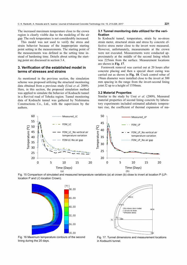
2.5 Verification of the model in terms of tem-perature Comparison of the simulated and the measured tempera-ture variations are shown in Fig. 15. It was observed that the measured temperature at crown was considera-bly higher than that at location P. It could be observed that the established model with assumptions could simu-late the temperature variations to an acceptable level. However, the temperature simulation at Location P was slightly overestimated.

The temperature simulation results without consider-ing the air gap at crown region and without assuming the vertical air temperature distribution (shown in Fig. 8) are also shown in Fig. 15. As shown in Fig. 15 (a), if the air gap was not modeled, the simulated crown tem-perature showed a considerable difference in the peak temperature. Similarly, if the air temperature distribu-tion in the vertical direction was not modeled, the simu-lated temperature distribution at the crown was consid-erably underestimated during the temperature decreas-ing period from about 3days onwards. However, as shown in Fig. 15 (b), temperature distribution simulated at location p overlapped in all three cases meaning that these assumptions did not affect the temperature varia-tion close to the invert.

Maximum temperature contours in the second lining during the analysis time of 20 days are shown in Fig. 16.

Table 6 Error in estimated maximum temperature.

Mesh Maximum Temperature (°C) Error Initial 55.04 -0.29%

Mesh-1 55.22 0.04% Mesh-2 55.2 _ Mesh-3 55.22 0.04%

20

30

40

50

60

0 5 10 15 20

Tempe

rature (0C)

Time (Days)

BE‐126‐Initial

CN‐32000‐Mesh‐1CN‐32000‐Mesh‐2CN‐3000‐Mesh‐3

‐1

0

1

0 5 10 15 20

Stress (N

/mm

2 )

Time (Days)

Initial‐Surface Initial‐InnerMesh‐3‐Surface Mesh‐3‐Inner

(a) (b) Fig. 13 Mesh sensitivity analysis. (a) Temperature variation at crown surface (b) Crown stress variation in initial and mesh-3 (surface – at lining surface. Inner – inside the second lining close to the waterproofing sheet).

‐0.5

0

0.5

1

1.5

2

0 5 10 15 20

Stress (N

/mm

2 )

Time (Days)

3DMesh‐1

3DMesh‐2

3DMesh‐3

Fig. 14 Comparison of longitudinal stresses of 3D meshes.


The increased maximum temperature close to the crown region is clearly visible due to the modeling of the air gap. The rock temperature is not considerably increased.

This model was not used to verify the stress and strain behavior because of the inappropriate starting point setting in the measurements. The starting point of the measurements was defined as the setting time in-stead of hardening time. Details about setting the start-ing point are discussed in section 3.4.

3. Verification of the established model in terms of stresses and strains

As mentioned in the previous section, the simulation scheme was proposed utilizing the structural monitoring data obtained from a previous study (Usui et al. 2009). Here, in this section, the proposed simulation method was applied to simulate the behavior of Kodsuchi tunnel in a Revival road of Tohoku region. Tunnel monitoring data of Kodsuchi tunnel was gathered by Nishimatsu Constructions Co., Ltd., with the supervision by the authors.

3.1 Tunnel monitoring data utilized for the veri-fication In Kodsuchi tunnel, temperature, strain by no-stress strain meter, structural strain and stress by concrete ef-fective stress meter close to the invert were measured. However, unfortunately, measurements at the crown were not executed. Measurements were conducted ap-proximately at the middle of the second lining which was 225mm from the surface. Measurement locations are shown in Fig. 17.

Formwork removal was carried out at 20 hours after concrete placing and then a special sheet curing was carried out as shown in Fig. 18. Crack control rebar of 19mm diameter were installed close to the invert at 300 mm spacing in the range from the invert-second lining joint J2 up to a height of 1550mm.

3.2 Material Properties Similar to the study by Usui et al. (2009), Measured material properties of second lining concrete by labora-tory experiments included estimated adiabatic tempera-ture rise, the coefficient of thermal expansion of ma-

20

25

30

35

40

45

50

55

60

0 5 10 15 20

Tempe

rature (0C)

Time (Days)

Measured_LC

FEM_LC

FEM_LC_No vertical airtemperature variation

FEM‐LC‐No air gap

20

25

30

35

40

45

50

0 5 10 15 20

Tempe

rature (0C)

Time (Days)

Measured_LP

FEM_LP

FEM_LP_No vertical airtemperature variation

FEM_LP_No air gap

(a) (b) Fig. 15 Comparison of simulated and measured temperature variations (a) at crown (b) close to invert at location P (LP- location P and LC-location Crown).

Fig. 16 Maximum temperature contours of the second lining during the 20 days.

Fig. 17. Tunnel dimensions and measurement locations in Kodsuchi tunnel.


tured concrete, and time-dependent development of compressive strength. The time-dependent tensile strength and Young’s modulus were not obtained from the laboratory experiments. Hence, the constants used in equation (2) and equation (3) were set based on the JCI standard (Japan Concrete Institute 2016). The material constants for the adiabatic temperature rise model shown in equation (4) were obtained from laboratory experiments and K =45.9, 1.91α = , 1β = , and t0 = 0.

The modification factor for creep deformation ( )teφ was calculated from the measurement data using equa-tion (8).

( )( )

( )

t Actualte

t JCI

EE

φ = (8a)

( )( )

( )

t efft Actual

t eff

Eσε

Δ=

Δ (8b)

( )( ) ( ) ( ) ( )t eff t Str t Temp t Volε ε ε ε= − + (8c)

( )t JCIE = the Young’s modulus calculated according to equation (3), ( )t ActualE = actual Young’s modulus of the structure at time step t, ( )t effσΔ = measured effective stress increment, ( )t effεΔ = calculated effective strain increment. Effective strains can be calculated by equa-tion (8c). ( )t Strε = measured structural strain, ( )t Tempε = temperature strain, and ( )t Volε = volumetric strain given by autogenous shrinkage in the current analysis. The quantity given by ( )( ) ( )t Temp t Volε ε+ can be directly ob-tained as the measurement from the no-stress strain me-ter.

The modification factor for creep deformation ( ( )teφ ) calculated from equation (8) for each time interval is

shown in Fig. 19 with the two constant values used in the simulation. In the modeling software, only two val-ues can be defined for the modification factor for creep in temperature increasing period and temperature de-creasing period. 0.88 was selected for temperature in-creasing period and 0.5 was selected for temperature decreasing period by observing the scattered calculation results. Mainly the calculated ( )teφ values before 7 days were considered for selecting appropriate ( )teφ because stress increment after that was very small.

The coefficient of thermal expansion measured in the laboratory was 6.22×10-6 °C-1. As the autogenous shrinkage of the concrete was not obtained from labora-tory tests, it was calculated using equation (9) from no-stress strain meter measurements assuming the constant coefficient of thermal expansion. Then the JCI autoge-nous shrinkage equation shown in equation (10) was scaled down to obtain the calculated autogenous shrink-age. The modification factor cη was set to 0.59 to ob-tain appropriate measured autogenous shrinkage strain. Calculated and used modified JCI model for autogenous

Plastic sheets

Fig. 18 Sheet curing in Kodsuchi tunnel.

intervals

Intervals

Up

Calculated

‐1

‐0.5

0

0.5

1

1.5

0 5 10 15 20

Mod

ificatio

n factor fo

r Creep(Ø(te))

Time (Days)

Creep factor Input Creep factor

to 0.6 Days‐1Hour Up to 2 Days‐6Hour intervals

to 7 Days‐12Hour Up to 20 Days‐48Hour Intervals Fig. 19 Calculated creep factors for each time interval using measured data and the two creep factors used for the simu-lation.


shrinkage are shown in Fig. 20. The initial part of the calculated autogenous shrinkage showed an expansion strain. However, this was thought to be due to the as-sumed constant coefficient of thermal expansion which might be smaller than the actual value in the initial stage. The calculated autogenous shrinkage was not directly used in the modeling because it will not simulate the temperature dependency of autogenous shrinkage.

( ) ( ) ( )t Vol t Nm Tε ε αΔ = Δ − Δ (9)

where, ( )t VolεΔ is the autogenous shrinkage strain in-crement, ( )t NmεΔ is the increment in the no-stress strain meter strain, TΔ is the temperature increment and α is the coefficient of thermal expansion.

( ) ( ) ( )sh te c sh sh teε η ε β∝= × × (10)

( )sh teε is the autogenous shrinkage at time et expressed in time adjusted age according to JCI standard. cη is the modification factor for cement type. ( )sh teβ Indicates the effect of time dependent development of autogenous shrinkage.

Due to the special sheet curing, the relative humidity close to the concrete surface was kept above 90% ac-cording to the measurements. Hence, the drying shrink-age was omitted from the simulation similar to the pre-vious case explained in section 2.

The initial concreting temperature was 26.5°C and the air temperature close to the invert was measured. All other material properties and initial conditions except for modeling of the reinforcing bars were set according to the modeling method proposed in Section 2. Regard-ing the analysis conditions such as time integration method, time step size and element size, these were set exactly equal to the analysis in section 2. Since the boundary conditions were not drastically different, it was expected that using the same settings should be appropriate.

3.3 Modeling of reinforcement It is known that reinforcement can be ignored in thermal stress analysis. However, for completeness, the crack control reinforcement was modeled using one-dimensional elements. Properties were set according to the JCI standard (Japan Concrete Institute 2016). The modeled reinforcing bars are shown in Fig. 21, and the constitutive law of 1D truss element is shown in Fig. 22. Respective properties used in 1D elements are listed in Table 7. The 1D truss elements should follow the nodes in the 3D mesh. In the actual structure, reinforcement was located with 300 mm spacing. In the model the re-bar was modeled with 200 mm spacing and the bar area was modified to maintain the actual reinforcement ratio.

3.4 Defining the starting time of the measure-ments and the simulation In the actual tunnel monitoring, the measurement was started after few minutes from the concrete placing. However, during the very initial period of early age concrete before hardening, it behaves as a plastic mate-rial with a very large coefficient of thermal expansion and a large deformation capability. The measured results before the hardening consist of very large strains and comparatively smaller stresses due to this plastic nature. These early stage measurements can also include unde-sirable strains due to formwork movement etc. Consid-

Table 7 Properties of one dimensional elements used for rebar.

Property Value Cross sectional area 1.91 cm2 Yielding stress ( yσ ) 250 N/mm2

Young’s modulus (E) 200000 N/mm2

Slope reduction factor after yielding (α) 0.001 Coefficient of thermal expansion (CTE) 10×10-6 °C-1

‐150

‐100

‐50

0

50

0 5 10 15 20

Strain(×

10‐6)

Time(Days)

Calculation

Modified JCI model

Fig. 20 Estimation of the autogenous shrinkage.

Second lining elements

Reinforcement modelled with 1Dtruss elements 1550 mm

Fig. 21 Modeling of reinforcement with 1D elements.

E

α×E yσ

σ (N/mm2)

ε

Fig. 22 Constitutive law of 1D elements.


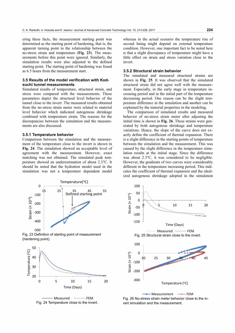
ering these facts, the measurement starting point was determined as the starting point of hardening, that is, the apparent turning point in the relationship between the no-stress strain and temperature (Fig. 23). The meas-urements before this point were ignored. Similarly, the simulation results were also adjusted to the defined starting point. The starting point of hardening was found as 6.5 hours from the measurement start.

3.5 Results of the model verification with Kod-suchi tunnel measurements Simulated results of temperature, structural strain, and stress were compared with the measurements. These parameters depict the structural level behavior of the tunnel close to the invert. The measured results obtained from the no-stress strain meter were related to material level behavior which indicated autogenous shrinkage combined with temperature strain. The reasons for the discrepancies between the simulation and the measure-ments are also discussed. 3.5.1 Temperature behavior Comparison between the simulation and the measure-ment of the temperature close to the invert is shown in Fig. 24. The simulation showed an acceptable level of agreement with the measurement. However, exact matching was not obtained. The simulated peak tem-perature showed an underestimation of about 2.3°C. It should be noted that the hydration model used in the simulation was not a temperature dependent model

whereas in the actual scenario the temperature rise of second lining might depend on external temperature condition. However, one important fact to be noted here is that a slight discrepancy of temperature might have a little effect on strain and stress variation close to the invert. 3.5.2 Structural strain behavior The simulated and measured structural strains are shown in Fig. 25. It was observed that the simulated structural strain did not agree well with the measure-ment. Especially, in the early stage in temperature in-creasing period and in the initial part of the temperature decreasing period. One reason can be the slight tem-perature difference in the simulation and another can be explained by the material properties in the modeling.

The comparison of simulated results and measured behavior of no-stress strain meter after adjusting the initial time is shown in Fig. 26. These strains were gen-erated by both autogenous shrinkage and temperature variations. Hence, the slope of the curve does not ex-actly define the coefficient of thermal expansion. There is a slight difference in the starting points of temperature between the simulation and the measurement. This was caused by the slight difference in the temperature simu-lation results at the initial stage. Since the difference was about 2.3°C, it was considered to be negligible. However, the gradients of two curves were considerably different in the temperature increasing period. This indi-cates the coefficient of thermal expansion and the ideal-ized autogenous shrinkage adopted in the simulation

‐500

‐400

‐300

‐200

‐100

015 25 35 45 55

Strain (×

10‐6)

Temperature(oC)

Defined starting point

Fig. 23 Definition of starting point of measurement (hardening point).

20

30

40

50

0 5 10 15 20

Tempe

rature (oC)

Time (Days)

Measured FEM Fig. 24 Temperature close to the invert.

‐150

‐100

‐50

0

50

100

0 5 10 15 20

Strain (×

10‐6)

Time (Days)

Measured FEM Fig. 25 Structural strain close to the invert.

‐300

‐200

‐100

0

100

20 25 30 35 40 45

Strain (×

10‐6)

Temperature (oC)

Measurement FEM Fig. 26 No-stress strain meter behavior close to the in-vert simulation and the measurement.


could not represent the material behavior sufficiently. The major part of this discrepancy might be due to the utilization of the constant coefficient of thermal expan-sion measured in matured concrete. In the initial stage, the coefficient of thermal expansion can be much larger.

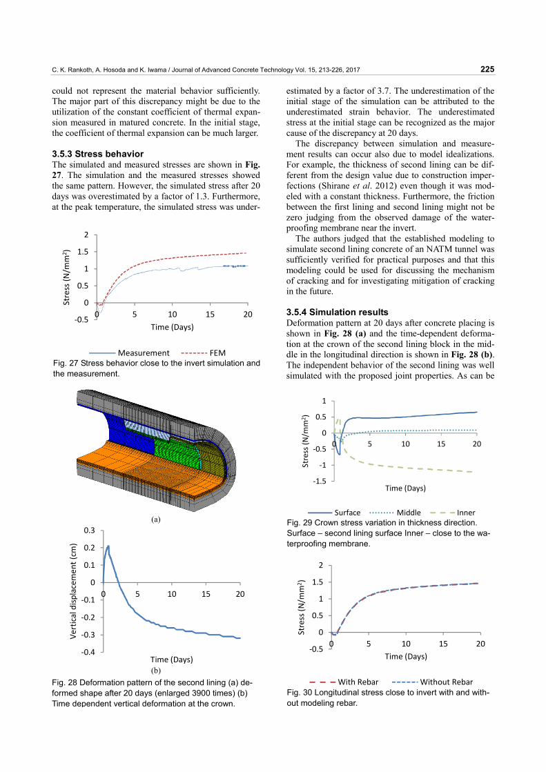
3.5.3 Stress behavior The simulated and measured stresses are shown in Fig. 27. The simulation and the measured stresses showed the same pattern. However, the simulated stress after 20 days was overestimated by a factor of 1.3. Furthermore, at the peak temperature, the simulated stress was under-

estimated by a factor of 3.7. The underestimation of the initial stage of the simulation can be attributed to the underestimated strain behavior. The underestimated stress at the initial stage can be recognized as the major cause of the discrepancy at 20 days.

The discrepancy between simulation and measure-ment results can occur also due to model idealizations. For example, the thickness of second lining can be dif-ferent from the design value due to construction imper-fections (Shirane et al. 2012) even though it was mod-eled with a constant thickness. Furthermore, the friction between the first lining and second lining might not be zero judging from the observed damage of the water-proofing membrane near the invert.

The authors judged that the established modeling to simulate second lining concrete of an NATM tunnel was sufficiently verified for practical purposes and that this modeling could be used for discussing the mechanism of cracking and for investigating mitigation of cracking in the future.

3.5.4 Simulation results Deformation pattern at 20 days after concrete placing is shown in Fig. 28 (a) and the time-dependent deforma-tion at the crown of the second lining block in the mid-dle in the longitudinal direction is shown in Fig. 28 (b). The independent behavior of the second lining was well simulated with the proposed joint properties. As can be

‐0.5

0

0.5

1

1.5

2

0 5 10 15 20

Stress (N

/mm

2 )

Time (Days)

Measurement FEM Fig. 27 Stress behavior close to the invert simulation and the measurement.

(a)

‐0.4

‐0.3

‐0.2

‐0.1

0

0.1

0.2

0.3

0 5 10 15 20

Vertical displacem

ent (cm

)

Time (Days) (b)

Fig. 28 Deformation pattern of the second lining (a) de-formed shape after 20 days (enlarged 3900 times) (b) Time dependent vertical deformation at the crown.

‐1.5

‐1

‐0.5

0

0.5

1

0 5 10 15 20

Stress (N

/mm

2 )

Time (Days)

Surface Middle Inner Fig. 29 Crown stress variation in thickness direction. Surface – second lining surface Inner – close to the wa-terproofing membrane.

‐0.5

0

0.5

1

1.5

2

0 5 10 15 20

Stress (N

/mm

2 )

Time (Days)

With Rebar Without Rebar Fig. 30 Longitudinal stress close to invert with and with-out modeling rebar.


seen from Fig. 28 (b), due to the assumption of the exis-tence of air gap close to the crown part, the top portion of the lining moved in vertically upward direction in temperature increasing period and then moved in vertically downward direction with the decrease of tem-perature and with the gravity load (gravity load was added into the simulation after 20 hours from the start).

Stress variations in the transverse direction at the crown are shown in Fig. 29.The stress near the surface of the second lining was in tension while the stresses of inner elements were in compression. A crack can occur at the crown if the tensile stress at the surface exceeds the tensile strength. However, this crack might be a non-penetrating crack in the thickness direction as the inner portion of the second lining is in compression. Similarly, when the stress distribution in thickness direction close to the invert was examined, it was observed that after 20 days tensile stresses were generated in the whole section which indicated a risk of generating a penetrating crack close to the invert.

Finally, the effect of modeling the crack control rebar close to the invert is shown in Fig. 30. As expected, modelling the reinforcing bars showed a negligible ef-fect on the longitudinal thermal stress. However, model-ing the reinforcing bars was thought to be essential in terms of future studies taking in to account the effect of drying shrinkage.

4. Conclusions

A modeling method was proposed for early age thermal stress analysis in second lining concrete of NATM tun-nels using finite element method. The modeling was sufficiently verified with field measurement data. Con-clusions that can be drawn from the study are as follows. 1. The sensitivity of the mesh size was not so large in

terms of thermal analysis. However, in terms of the stress in the longitudinal direction, mesh sensitivity was not negligible.

2. The early age temperature behaviors could be simu-lated to an acceptable level based on the thermal properties suggested for the waterproofing sheet in-cluding the existence of air void, and based on other conditions such as thermal boundary conditions and the modeled thickness of the rock.

3. The modeling of air void close to the crown and the modeling of the vertical air temperature distribution were indispensable to simulate the proper tempera-ture variation of the second lining concrete.

4. Assumed joint conditions could simulate the inde-pendent behavior of second lining to an acceptable level.

5. Important inputs related to early thermal stress such as effective Young’s modulus, autogenous shrinkage development, and setting of hardening time were proposed based on measurement results. The slight difference between the simulation results and the measurement could be explained by the imperfec-

tions of the tunnel lining as well as by the idealiza-tions made in the modeling.

6. From the simulated stress results, it was observed that the crown cracks might be non-penetrating cracks while the cracks close to invert might be pene-trating cracks.

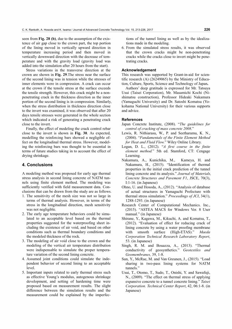
Acknowledgement This research was supported by Grant-in-aid for scien-tific research (A) (26249065) by the Ministry of Educa-tion, Culture, Sports, Science and Technology of Japan.

Authors’ deep gratitude is expressed for Mr. Tatsuya Usui (Taisei Corporation), Mr. Masamichi Kochi (Ni-shimatsu construction), Professor Hideaki Nakamura (Yamaguchi University) and Dr. Satoshi Komatsu (Yo-kohama National University) for their various supports and advice.

References Japan Concrete Institute, (2008). “The guidelines for

control of cracking of mass concrete 2008.” Lewis, R. Nithiarasu, W., P. and Seetharamu, K. N.,

(2004). “Fundamentals of the Finite Element Method for Heat and Fluid Flow.” Wiley Online Library.

Logan, D. L., (2012). “A first course in the finite element method.” 5th ed. Stamford, CT: Cengage Learning.

Nakamura, A., Kunichika, M., Kameya, H. and Nakamura, H., (2015). “Identification of thermal properties in the initial crack prediction of the tunnel lining concrete and its analysis.” Journal of Materials, Concrete Structures and Pavement F1, JSCE, 70(3), I:1-16. (in Japanese)

Ohno, U. and Hosoda, A., (2012). “Analysis of database of actual structures in Yamaguchi Prefecture with thermal stress simulation.” Proceedings of JCI, 34(1), 1288-1293. (in Japanese)

Research Center of Computational Mechanics. Inc., (2015). “ASTEA MACS for Windows Ver. 8 User manual.” (in Japanese)

Shirane, Y., Kagawa, M., Kikuchi, A. and Komatsu, T., (2012). “Evaluation of effect for reducing crack of lining concrete by using a water proofing membrane with smooth surface (High-ETAS).” Maeda Corporation Technical Research Laboratory Report, 53. (in Japanese)

Singh, R. M. and Bouazza, A., (2013). “Thermal conductivity of geosynthetics.” Geotextiles and Geomembranes, 39, 1-8.

Sun, Y., McRae, M. and Van Greunen, J., (2015). “Load sharing in two-pass lining systems for NATM tunnels.”

Usui, T., Otomo, T., Sudo, T., Onishi, Y. and Sawafuji, N., (2009). “The effect on thermal stress of applying expansive concrete to a tunnel concrete lining.” Taisei Corporation. Technical Center Report, 42, 06:1-8. (in Japanese)

modeling and verification of early age thermal stress in

Documents