modeling sequential information acquisition behavior in ...tavana.us/publications/ds-sia.pdf ·...
TRANSCRIPT
Decision SciencesVolume 47 Number 4August 2016
© 2016 Decision Sciences Institute
Modeling Sequential InformationAcquisition Behavior in Rational DecisionMaking∗Madjid Tavana†Business Systems and Analytics Department, Distinguished Chair of Business Analytics, LaSalle University, Philadelphia, PA 19141 and Business Information Systems Department,Faculty of Business Administration and Economics, University of Paderborn, D-33098Paderborn, Germany, e-mail: [email protected]
Debora Di CaprioDepartment of Mathematics and Statistics, York University, Toronto M3J 1P3, Canada andPolo Tecnologico IISS G. Galilei, Via Cadorna 14, 39100, Bolzano, Italy,e-mail: [email protected]
Francisco J. Santos ArteagaDepartamento de Economıa Aplicada II, Facultad de Economicas, Universidad Complutensede Madrid, Campus de Somosaguas, 28223 Pozuelo, Spain, e-mail: [email protected]
ABSTRACT
Most real-life decisions are made with less than perfect information and there is oftensome opportunity to acquire additional information to increase the quality of the deci-sion. In this article, we define and study the sequential information acquisition processof a rational decision maker (DM) when allowed to acquire any finite amount of in-formation from a set of products defined by vectors of characteristics. The informationacquisition process of the DM depends both on the values of the characteristics observedpreviously and the number and potential realizations of the remaining characteristics.Each time an observation is acquired, the DM modifies the probability of improvingupon the products already observed with the number of observations available. We con-struct two real-valued functions whose crossing points determine the decision of how toallocate each available piece of information. We provide several numerical simulationsto illustrate the information acquisition incentives defining the behavior of the DM. Ap-plications to knowledge management and decision support systems follow immediatelyfrom our results, particularly when considering the introduction and acceptance of new
∗The authors would like to thank the anonymous reviewers and the editor for their insightful comments andsuggestions.
Subject Classification Scheme for the OR/MS Index: Decision analysis (risk, sequential); Util-ity/preference (multiattribute); Information systems (decision support systems).
†Corresponding author.
720
Tavana, Di Caprio, and Arteaga 721
technological products and when formalizing online search environments. [Submitted:December 15, 2014. Revised: September 15, 2015. Accepted: October 20, 2015.]
Subject Areas: Forward-Looking Behavior, Rationality, Search Process,Sequential Information Acquisition, and Utility.
INTRODUCTION
Consider a situation where a decision maker (DM) has to check a finite numberof characteristics from a set of two dimensional products. In the words of Beardenand Connolly (2007), a DM must “continuously decide when to stop searchingwithin an option—to get a better estimate of its value—and when to stop searchingbetween options—to find one of high value. Striking a balance between depth(within-option) and breadth (between-option) search presents a complex problem.”
The standard information acquisition process generally considered bythe operations research and management literatures is described in Figure 1.The subscripts of each observation denote the characteristic of the product, ei-ther the first or the second. Each superscript indicates the product being observedafter the initial one. In particular,m refers to the second product observed,m+ 1 tothe third one, and so on. Whenever a DM acquires information sequentially he mustchoose between continuing with the latest product observed (upper arrow leavingfrom each node when a choice must me made) or start acquiring information on anew product (lower arrow leaving from each node).
The first characteristic of a product has been assumed to be more importantthan the second one, leading the DM to start acquiring information on the firstcharacteristic of each new product instead of the second one. This is the casebecause acquiring information on the first characteristic provides a higher expectedutility than doing so on the second, as follows trivially from the informationacquisition context that will be described in the article.
The behavior of the DM and the resulting stopping rule depend on the ex-pected value derived from the next characteristic to be observed and the informationacquisition costs faced by the DM. The DM rarely considers recalling previouspartially observed products and the information acquisition algorithm does not de-pend on the number of observations remaining to be acquired or the set of potentialimprovements that may be realized relative to the products previously observed.The inclusion of these search features is particularly important when analyzingonline search environments, where the costs of recalling a previous alternativeamong those displayed by the search engine is considerably low. On the otherhand, the cognitive costs required on the side of the DM increase substantiallydepending on the amount of information that must be acquired and the capacity ofthe DM to assimilate this information.
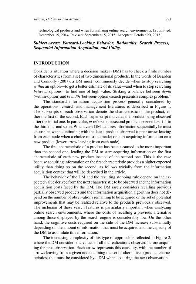
The increasing complexity of this type of approach is reflected in Figure 2,where the DM considers the values of all the realizations observed before acquir-ing the next observation. Each arrow represents this causality, with the number ofarrows leaving from a given node defining the set of alternatives (product charac-teristics) that must be considered by a DM when acquiring the next observation.

722 Modeling Sequential Information Acquisition Behavior
Figure 1: Standard sequential information acquisition process—absent recall andindependent from the number of observations remaining to be acquired.
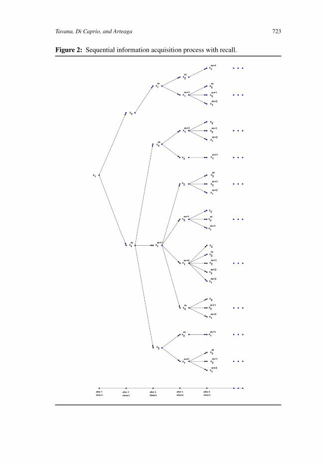
At the same time, when defining his information acquisition process, theDM should consider the number and potential realizations of all the remainingobservations, together with the probability that they lead to a product deliveringa higher utility than the best among the observed ones. In order to illustrate thecomplexity and nonrecursivity of the information acquisition process that mustbe defined by the DM, consider the space of potential realizations that should beanalyzed when a total of two observations are acquired. Figure 3 illustrates thisscenario.
In this case, before deciding how to allocate his second (and final) observa-tion, the DM must account for all the combinations of the first observation froman initial product, x1, with both the second characteristic of this product, x2, andthe first characteristic from a new product, xm1 .
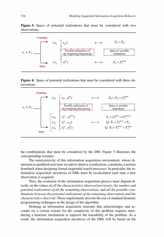
A similar, though more complex, intuition follows from a setting where theDM acquires three observations. As illustrated in Figure 4, the space of potentialrealizations that must be analyzed when three observations are acquired becomesmore complex because a larger amount of potential combinations must be consid-ered by the DM.
Note how each new observation produces a set of possible combinations thatmust be accounted for by the DM when acquiring the first observation. Despitethis fact, the setting with three observations can still be analyzed within a threedimensional space that determines the information acquisition incentives of theDM based on all the potential realizations of x1 andxm1 .
However, the set of potential realizations that must be analyzed when fourobservations are acquired requires a higher dimensional space to account for
Tavana, Di Caprio, and Arteaga 723
Figure 2: Sequential information acquisition process with recall.
724 Modeling Sequential Information Acquisition Behavior
Figure 3: Space of potential realizations that must be considered with twoobservations.
Figure 4: Space of potential realizations that must be considered with three ob-servations.
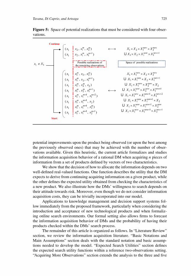
the combinations that must be considered by the DM. Figure 5 illustrates thecorresponding scenario.
The nonrecursivity of this information acquisition environment, whose di-mension is modified each time we add or observe a realization, constitutes a seriousdrawback when designing formal sequential search processes. In particular, the in-formation acquisition incentives of DMs must be recalculated each time a newobservation is acquired.
Thus, the evolution of the information acquisition process must depend di-rectly on the values of all the characteristics observed previously, the number andpotential realizations of all the remaining observations, and all the possible com-binations between the potential realizations of the remaining observations and thecharacteristics observed. These requirements prevent the use of standard dynamicprogramming techniques in the design of the algorithm.
Defining an information acquisition structure that acknowledges and ac-counts (to a certain extent) for the complexity of this problem requires intro-ducing a heuristic mechanism to improve the tractability of the problem. As aresult, the information acquisition incentives of the DMs will be based on the
Tavana, Di Caprio, and Arteaga 725
Figure 5: Space of potential realizations that must be considered with four obser-vations.
potential improvements upon the product being observed (or upon the best amongthe previously observed ones) that may be achieved with the number of obser-vations available. Given this heuristic, the current article formalizes and studiesthe information acquisition behavior of a rational DM when acquiring n pieces ofinformation from a set of products defined by vectors of two characteristics.
We show that the decision of how to allocate the information depends on twowell-defined real-valued functions. One function describes the utility that the DMexpects to derive from continuing acquiring information on a given product, whilethe other defines the expected utility obtained from checking the characteristics ofa new product. We also illustrate how the DMs’ willingness to search depends ontheir attitude towards risk. Moreover, even though we do not consider informationacquisition costs, they can be trivially incorporated into our model.
Applications to knowledge management and decision support systems fol-low immediately from the proposed framework, particularly when considering theintroduction and acceptance of new technological products and when formaliz-ing online search environments. Our formal setting also allows firms to forecastthe information acquisition behavior of DMs and the probability of having theirproducts checked within the DMs’ search process.
The remainder of this article is organized as follows. In “Literature Review”section, we review the information acquisition literature. “Basic Notations andMain Assumptions” section deals with the standard notation and basic assump-tions needed to develop the model. “Expected Search Utilities” section definesthe expected search utility functions within a reference two-observations setting.“Acquiring More Observations” section extends the analysis to the three and five
726 Modeling Sequential Information Acquisition Behavior
observations environments while “The Proposed Information Acquisition Struc-ture with n Observations” section defines the information acquisition structurewhen any finite number of observations can be acquired by the DM. “Framingand Reference Products” section illustrates the consequences from modifying thereference product employed in the design of the algorithm. “The Information Ac-quisition Process” section describes the sequential information acquisition processof the DM. “Conclusions and Managerial Significance” section summarizes themain findings and highlights their managerial significance. An elaborate examplebased on the results displayed by an online search engine when the DM acquiresa total of five observations is presented in the Online Appendix.
LITERATURE REVIEW
The elimination of uncertainty and its transformation into risk provides themain motivation for the development of information acquisition algorithms (DiCaprio, Santos Arteaga, & Tavana, 2014b). The design and study of algorithmicinformation acquisition processes constitutes one of the main focuses of the oper-ations research literature (MacQueen & Miller, 1960; MacQueen, 1964). Indeed,the management and operations research literatures have been considering the op-timal information gathering problem of DMs for quite some time, in particularwhen analyzing the acquisition of a new technology (McCardle, 1985; Lippman &McCardle; 1991). These authors build rational information gathering algorithmswhere the decision of which information to acquire is based on the utility gainsexpected to be obtained by the DM. The use of dynamic programming techniquesto illustrate the existence of optimal decision threshold values requires imposingseveral formal restrictions on the corresponding return functions. These constraintshelp understand the structural complexities involved in designing optimal infor-mation acquisition and evaluation processes.
This research line remains focused on the importance that search costs havein limiting the information processing capacity of generally risk neutral DMs whendeciding whether to continue or to stop their search within settings defined by theacceptance of a given investment opportunity or the adoption of a technology(Levesque & Maillart, 2008; Ulu & Smith, 2009; Smith & Ulu, 2012). Extensionsof this framework are provided by Shepherd and Levesque (2002), who endow theDM with basic memory capacities when computing the evolution of the expectedprofits derived from a given business opportunity. At the same time, the decisiontheoretical branch of operations research has also extended this type of models toallow for comparisons between different technologies (Cho & McCardle, 2009;Kwon, 2010).
Consider now the potential applications of these information acquisitionmodels within the decision support and consumer choice literatures. As was thecase with their theoretical counterparts, applications of multi-attribute informationacquisition algorithms to these branches of the literature rely on simplifying mech-anisms that allow for the use of dynamic programming techniques to obtain optimalsequential choice policies. For example, Feinberg and Huber (1996) implementeda screening heuristic limiting the number of alternatives evaluated by the DM.

Tavana, Di Caprio, and Arteaga 727
Lim, Bearden, and Smith (2006) eliminated recall and concentrated on linear ad-ditive value functions. Bearden and Connolly (2007) accounted for the sequentialinformation acquisition structure determining the search process of DMs but didnot derive the corresponding optimal thresholds or analyze their behavior. Thisis also the case in Wilde (1980) when defining the optimal choice behavior of aDM for the search and experience characteristics of two dimensional products andin Ratchford (1982) when considering deviations from an unidentified optimumchoice value.
A considerable amount of research relates to the applicability of informationacquisition algorithms in the design of tools that customize the online shoppingenvironment to the individual preferences of DMs (Haubl & Trifts, 2000). Themain lines of research opened by management scholars find their way into thedecision support literature dealing with online search environments. In this regard,this literature concentrates on creating decision support tools that allow the DM tocompare attributes among different online alternatives (Abrahams & Barkhi, 2013).At the same time, Browne, Pitts, and Wetherbe (2007) illustrate how DMs stopsearching for information online depending on the search task being performed.From a supply perspective, Wang, Wei, and Chen (2013) proposed a methodto estimate the probability that a product is considered for purchase after beinginspected by a consumer, while Dou, Lim, Su, Zhou, and Cui (2010) analyzed howfirms can employ their ranking position in the result pages of online search enginesto differentiate their products from those of the competitors.
BASIC NOTATIONS AND MAIN ASSUMPTIONS
The main assumptions on which the expected search utilities are built correspondto those described by Di Di Caprio, Santos Arteaga, and Tavana (2014a). In orderto keep the current article self-contained, we restate them below.
Let X be a nonempty set and � a preference relation defined on X. A utilityfunction representing a preference relation � on X is a function u : X → � suchthat
∀x, y ∈ X, x �∼ y ⇔ u(x) ≥ u(y). (1)
We use the symbol ≥ to denote the standard partial order on the reals. WhenX ⊆ � and � coincides with ≥, we say that u is a utility function on X.
Henceforth, G will denote the set of all products. We let X1 and X2, respec-tively, represent the sets of all possible variants for the first and second character-istics of a product in G. Also, X = X1 ×X2, so that every product in G can bedescribed by a pair < x1, x2 > in X. Note that, Xk is called the kth characteristicfactor space, with k = 1, 2, while X stands for the characteristic space.
We work under the following assumptions.
Assumption 1: For every k = 1, 2, there exist αk , βk > 0, with αk �= βk , suchthat Xk = [αk, βk], where αk and βk are the minimum and maximum of Xk .
Assumption 2: The characteristic space X is endowed with a strict preferencerelation �.
728 Modeling Sequential Information Acquisition Behavior
This assumption guarantees the rationality of the DM. The model introducedin this article requires the DM to be endowed only with a standard strict preferencerelation (complete and transitive, thus, rational; Mas-Colell, Whinston, & Green,1995) that allows him to order the set of products and choose between two of them.
Assumption 3: There exist a continuous additive utility function u representing� on X such that each one of its components uk : Xk → �, where k = 1, 2 is acontinuous utility function onXk . A utility function u : X → � representing � onX = X1 ×X2 is called additive (Wakker, 1989) if there exist uk : Xk → �, wherek = 1, 2, such that ∀ < x1, x2 >∈ X1 ×X2, u(< x1, x2 >) = u1(x1) + u2(x2).
The sequential property of the information acquisition process provides anintuitive justification for the additive separability assumption imposed on the utilityfunction. However, it seems perfectly reasonable to consider products whose com-plementarity among characteristics requires a nonseparable utility representation.An immediate example could relate to the purchase of a house, whose evaluationdoes not only depend on features related to the house itself but also to externallocation type factors, both of which are usually interrelated. In this sense, therelationship between both types of characteristics could be interpreted such thatthe second dimension represents the portion of the second characteristic that is notexplained by the first one. In this regard, as illustrated by Tavana, Di Caprio, andSantos Arteaga (2014), each characteristic can also be interpreted as a category ac-counting for different related properties of a product. As a result, search processeswould be defined by observable (X1) and experience (X2) components, the latterrequiring a more detailed inspection of the product to be verified (Nelson, 1970).
Assumption 4: For every k = 1, 2, μk : Xk → [0, 1] is a continuous probabilitydensity on Xk , whose support, the set {xk ∈ Xk : μk(xk) �= 0}, will be denoted bySupp(μk).
The probability densities μ1 and μ2 represent the subjective “beliefs” of theDM. That is, for k = 1, 2, μk(Yk) is the subjective probability that a randomlyobserved product fromG displays an element xk ∈ Yk ⊆ Xk as its kth characteris-tic. The probability densities μ1 and μ2 are assumed to be independent. However,the information acquisition structure described in the article allows for subjectivecorrelations to be defined between different characteristics within a given prod-uct. Considering a correlated environment would not modify the main theoreticalstructure built in the article though it would lead to different quantitative resultsthrough the numerical simulations.
Note that the characteristics and probabilities associated with different prod-ucts depend on the type of product under consideration. For example, the char-acteristics that are important to a DM when choosing a laptop computer may bequite different from those considered when choosing a desktop one. It should beemphasized that the DM will not solve a classic optimization problem but searchesfor a sufficiently good product given his subjective preferences and beliefs. In thissense, our model is in line with the empirical psychological literature on consumerchoice based on bounded rationality and the limited capacity of DMs to assimilateall the information available (Samiee, Shimp, & Sharma, 2005; Diab, Gillespie, &Highhouse, 2008)
Tavana, Di Caprio, and Arteaga 729
Finally, following the standard economic theory of choice under uncertainty,we assume that the DM elicits the kth certainty equivalent (CE) value induced byμkand uk as the reference point against which to compare the information collected onthe kth characteristic of a given product. Given k = 1, 2, the certainty equivalentof μk and uk , denoted by cek , is a characteristic in Xk that the DM is indifferent toaccept in place of the expected one to be obtained through μk and uk . That is, forevery k = 1, 2, cek = u−1
k (Ek), where Ek denotes the expected value of uk . Theexistence and uniqueness of the kth CE value cek are guaranteed by the continuityand strict increasingness of uk , respectively.
EXPECTED SEARCH UTILITIES
Two Observations Reference Setting
The set of all products, G, is identified with a compact and convex subset of the2-dimensional real space �2. In the current setting, after observing the value of thefirst characteristic from an initial product, the DM has to decide whether to checkthe second characteristic from the same product, or to check the first characteristicfrom a different new product. In this regard, DMs are tacitly assumed to have awell-defined preference order both within and between characteristics. That is, thefirst characteristic will be assumed to be more important and, as a result, providea higher expected utility to the DM than the second one.
We show below that the decision of how to allocate the second availablepiece of information depends on two real-valued functions defined onX1. The DMconsiders the sum E1 + E2, corresponding to the expected utility values of thepairs < u1, μ1 > and < u2, μ2 >, as the main reference value when calculatingboth these functions.
Assume that the DM has already checked the first characteristic from aninitial product, x1, and that he uses his remaining piece of information to observethe second characteristic from this product, x2. Clearly, the expected utility gainover E1 + E2 varies with the value of x1 observed. That is, for every x1 ∈ X1, let
P+(x1) = { x2 ∈ X2 ∩ Supp(μ2) : u2(x2) > E1 + E2 − u1(x1)} (2)
and
P−(x1) = { x2 ∈ X2 ∩ Supp(μ2) : u2(x2) ≤ E1 + E2 − u1(x1)} , (3)
where P+(x1) and P−(x1) define the set of x2 values from the initial productsuch that their combination with x1 delivers a higher or lower equal utility than arandomly chosen product from G, respectively.
Let F : X1 → � be defined by
F (x1)def=∫P+(x1)
μ2(x2) (u1(x1) + u2(x2)) dx2 +∫P−(x1)
μ2(x2) (E1 + E2) dx2,
(4)
where F (x1) describes the DM’s expected utility derived from checking the secondcharacteristic of the initial product after observing that the value of the first char-acteristic is given by x1. Note that, if u1(x1) + u2(x2) ≤ E1 + E2, then choosing a

730 Modeling Sequential Information Acquisition Behavior
product fromG randomly delivers an expected utility ofE1 + E2 to the DM, whichis higher than the utility obtained from choosing the initially observed product,that is, u1(x1) + u2(x2).
Consider now the expected utility that the DM could gain over the initial(partially observed) product if the second piece of information is used to observethe first characteristic from a different product, xm1 . For every x1 ∈ X1, defineH : X1 → � as follows:
H (x1)def= (u1(x1) + E2) + C, (5)
where
Cdef= μ1
(xm1 ≤ x1
)(E1 + E2) + μ1
(xm1 > x1
)(u1(xm1)+ E2
). (6)
H (x1) describes the expected utility derived from checking the first characteristicof a new product after observing x1. If xm1 ≤ x1, then the new product observed bythe DM does not deliver a higher utility than the initial one and the payoff obtainedfrom such an event is set equal to E1 + E2. This reference value has been chosento generate a similar payoff environment to the one defined by the function F (x1).
Note however that the payoffs assigned to the x1 > xm1 ≥ ce1 and the ce1 >
xm1 > x1 outcomes within C may seem counterintuitive. In the former case, thenew observation is located above the CE value but does not improve upon theinitial product, leading to a payoff of E1 + E2. A similar intuition applies whenconsidering the latter case, with the new observation located below the CE value butits expected utility accounted for as a payoff (because xm1 > x1). We will analyzethe main consequences derived from modifying the reference values consideredby the DM in “Framing and Reference Products” section.
The current approach to the information acquisition behavior of DMs con-siders only potential improvements relative to the initial reference product, whosevalue is determined by x1. In this case, the function F (x1) completely eliminatesany uncertainty regarding the initial product, while DMs only observe the initialproduct partially withinH (x1). However, the functionH (·) allows for an additionalproduct to be observed relative to F (·). This observational advantage distorts theincentives of DMs when a small number of observations is considered, with largeramounts eliminating the resulting effect, as intuition prescribes and the numericalsimulations will illustrate.
In order to account for the set of potential improvements based on the numberof remaining observations, we rewrite the expression for C within H (x1) in thefollowing way:
C = ψ1(1, 0, μ1) (E1 + E2) + ψ1(1, 1, μ1)(u1(xm1)+ E2
). (7)
We will motivate this notational modification in the following section.Finally, note that the expected search utilities F and H determine the in-
formation acquisition behavior of the DM. That is, after observing x1, the DMwill either continue acquiring information on the initial product or start acquiringinformation on a new one depending on whether it is F or H the function takingthe highest value at x1. It may also happen that F (x∗
1 ) = H (x∗1 ) at a given x∗
1 ∈ X1,making the DM indifferent between continuing with the initial product and
Tavana, Di Caprio, and Arteaga 731
starting with a new one. These x∗1 values behave as information acquisition thresh-
olds that partition X1 in subintervals whose values induce the DM to either con-tinue acquiring information on the initial product or to switch and start observing anew one.
Numerical Simulations
This section presents numerical simulations that illustrate the information acqui-sition behavior of DMs when acquiring two observations. Simulations will beprovided for risk neutral and risk averse DMs, while keeping in mind that a largeset of potential scenarios can be studied numerically following the theoreticalsetting introduced in the article.
Consider, as the basic reference cases, the two observations acquisition be-havior that follows from a standard risk neutral and a risk averse utility func-tion when uniform probabilities are assumed on both X1 and X2. The followingparameter values will be used in all the numerical simulations presented in thearticle:
(i) Characteristic spaces: X1 = [5, 10], X2 = [0, 10];
(ii) Risk neutral utility functions: ∀x1 ∈ X1, u1(x1) = x1; ∀x2 ∈ X2,u2(x2) = x2;
(iii) Risk averse utility functions: ∀x1 ∈ X1, u1(x1) = √x1; ∀x2 ∈ X2,
u2(x2) = √x2;
(iv) Risk seeking utility functions: ∀x1 ∈ X1, u1(x1) = (x1)3/2; ∀x2 ∈ X2,u2(x2) = (x2)3/2;
(v) Probability densities: ∀x1 ∈ X1, μ1(x1) = 15 ; ∀x2 ∈ X2, μ2(x2) = 1
10 .
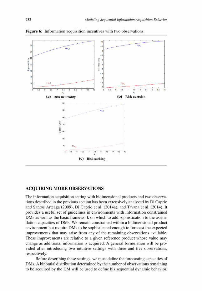
The basic reference risk neutral, risk averse and risk seeking settings are rep-resented in Figures 6a–c, respectively. In all figures, the horizontal axis representsthe set of x1 realizations that may be observed by the DM, with the correspondingsubjective expected utilities defined on the vertical axis. Observe the completedominance of the function H (x1) over F (x1) when two observations are consid-ered. As we will see through the rest of the numerical simulations, this initial effectwears off as a higher number of observations become available to the DM. Clearly,when only two observations are acquired, continuing with the initial product ob-served implies ending up with a unique product: either the initial one if it providesa utility higher than 〈ce1, ce2〉 or a randomly chosen product if the utility derivedfrom the initial one is below that of 〈ce1, ce2〉.
However, when acquiring information on a new product, the DM will havetwo products to choose from, the initial and a new one, both partially observed.The new product is added to the total utility of the DM, biasing his incentivestowards observing a product other than the initial one. This effect is eliminated inDi Caprio and Santos Arteaga (2009), where a unique final product is accounted forin the choice set of DMs through both functions F and H . The current frameworkis designed to accommodate a large amount of potential observations and it is tobe treated as such, with a large bias towards diversification arising when a smallnumber of observations are acquired.
732 Modeling Sequential Information Acquisition Behavior
Figure 6: Information acquisition incentives with two observations.
ACQUIRING MORE OBSERVATIONS
The information acquisition setting with bidimensional products and two observa-tions described in the previous section has been extensively analyzed by Di Caprioand Santos Arteaga (2009), Di Caprio et al. (2014a), and Tavana et al. (2014). Itprovides a useful set of guidelines in environments with information constrainedDMs as well as the basic framework on which to add sophistication to the assim-ilation capacities of DMs. We remain constrained within a bidimensional productenvironment but require DMs to be sophisticated enough to forecast the expectedimprovements that may arise from any of the remaining observations available.These improvements are relative to a given reference product whose value maychange as additional information is acquired. A general formulation will be pro-vided after introducing two intuitive settings with three and five observations,respectively.
Before describing these settings, we must define the forecasting capacities ofDMs. A binomial distribution determined by the number of observations remainingto be acquired by the DM will be used to define his sequential dynamic behavior.
Tavana, Di Caprio, and Arteaga 733
The probability that l among the remaining n observations improve upon theobserved characteristic x1 and deliver an expected product better than the one thathas been partially observed is given by the following binomial distribution:
ψ1(n, l, μ1
(xm1 > x1
)) =(n
l
)μ1(xm1 > x1
)l(1 − μ1
(xm1 > x1
))n−l, (8)
where μ1(xm1 > x1) is the probability that a new randomly selected product isendowed with a better first characteristic than the currently observed one, whichis endowed with x1. Similarly, when the second characteristic is considered, allpossible combinations delivering an improvement over the initial partially observedproduct should be accounted for
ψ2(n, l, μ2(xm2 ∈ P+(x1)))=(n
l
)μ2(xm2 ∈ P+(x1))l(1−μ2(xm2 ∈P+(x1)))n−l ,(9)
where μ2(xm2 ∈ P+(x1)) is the probability that a new randomly selected producthas a second characteristic belonging to the set P+(x1) determined by the observedx1 realization.
The combination ofψ1(n, l, μ1(xm1 > x1)) andψ2(n, l, μ2(xm2 ∈ P+(x1)))determines the probability that a randomly selected product is endowed with anexpected set of characteristics from X1 and X2 better than the partially observedproduct defined by (x1, P
+(x1)). In order to simplify notation, we will refer to boththese binomials by ψ1(n, l, μ1) and ψ2(n, l, μ2), respectively, while accountingfor the corresponding values of n and 1. Moreover, we will allow for the initialreference points to be modified in “Framing and Reference Products” section,where the notation will be adjusted accordingly.
The Proposed Information Acquisition Structure with ThreeObservations
The information acquisition scenario with three observations is introduced toprovide some basic intuition on the transition from the two observations setting toa general one with a total of n observations.
Consider the information acquisition problem faced by a DM after havinggathered the first observation from an initial product, given by x1, when a totalof three observations can be acquired. In this case, the DM must calculate twoenhanced versions of the original functions F (x1) and H (x1). These new func-tions must account for the two observations left to be acquired by the DM andthe probability that such observations provide a product better than the initiallyobserved one, which will be used through this section and the following one asthe main reference value. When calculating the enhanced function F (x1), we mustaccount for the fact that the DM uses the second piece of information available toacquire x2 and observe the initial product fully, that is, the DM observes 〈x1, x2〉.As a result, the payoff obtained by the DM depends on the expected realization ofx2 and that of xm1 , that is, the first characteristic from the new product observed,with the following combinations being considered regarding the third and finalobservation:

734 Modeling Sequential Information Acquisition Behavior
(1-0) This option corresponds to the subcase defined by the binomial probabil-ity ψ1(1, 0, μ1). It implies that after fully observing the initial product,the final observation xm1 does not provide a characteristic higher than x1.As a result, because the final observation does not improve upon the initialone and the DM has not yet observed x2, the expected outcome followingfrom this event is defined by the CE product: ψ1(1, 0, μ1)(E1 + E2).That is, the default payoff derived from an unsuccessful search is as-sumed to be given by the CE product.
(1-1) This option corresponds to the subcase defined by the binomial probabil-ity ψ1(1, 1, μ1). It implies that after fully observing the initial product,the final observation xm1 provides a characteristic higher than x1. As aresult, because the final observation improves upon the initial one andthe DM has not yet observed x2, the expected outcome following fromthis event is given by ψ1(1, 1, μ1)(u1(xm1 ) + E2).
When defining the enhanced version of function H (x1), we must accountfor the fact that the DM has one more observation left to acquire than in theF (x1) setting, because the second observation has not been used to acquire x2.Thus, the sets of possible combinations that must be considered when definingthe enhanced versions of function H (x1) always include one observation morethan those defining the enhanced F (x1) setting. The following combinations arisefrom the set of two observations that the DM has left to acquire within the currentsetting, with the notation describing the same type of sequential pattern as the oneintroduced in the subcases above.
(2-0) This option implies that none of the two observations left provides axm1 > x1. Therefore, the expected outcome following from this event isdefined by the CE product: ψ1(2, 0, μ1)(E1 + E2).
(2-1) This option implies that only one of the two observations left provides axm1 > x1. It also implies that the observation leading to xm1 > x1 must bethe second one. That is, if the observation providing xm1 > x1 would havebeen the first one, then the second observation would have been used bythe DM to acquire xm2 , leading to the (1-1) subcase described below. Thus,the DM ends up with a partially observed product 〈xm1 , ce2〉 The resultingexpected payoff is therefore given by: ψ1(2, 1, μ1)(u1(xm1 ) + E2).
(1-1) This option implies that the first observation acquired leads to acharacteristic xm1 > x1, which allows the DM to use the remainingobservation to acquire xm2 , that is, the second characteristic fromthe new product observed. This is trivially the optimal way to pro-ceed because xm1 > x1 and all second characteristics are equally dis-tributed. Note that the set of possible outcomes derived from observ-ing xm2 is defined by (1-0) and (1-1). The resulting expected payoff istherefore given by ψ1(1, 1, μ1)[ψ2(1, 1, μ2)
(u1(xm1)+ u2
(xm2))+
ψ2(1, 0, μ2)(E1 + E2)].
Even though we will modify the reference points defining the correspondingenhanced functions F (x1) and H (x1) and allow for alternative payoff scenarios
Tavana, Di Caprio, and Arteaga 735
based on the expected realizations of x2 in “Framing and Reference Products”section, several comments are due now. The basic reference product upon which theDM is expected to improve through the information acquisition process is given by(x1, P
+(x1)). That is, the characteristic initially observed determines the referencepoint on which the information acquisition process is based. The consequencesfor the information acquisition process of DMs will become evident below, as wedescribe the different sections composing the algorithm. The intuitive explanationfor this assumption may range from framing and context effects together withoptimism or pessimism on the side of the DMs (Kahneman & Tversky, 2000;Novemsky, Dhar, Schwarz, & Simonson, 2007) to subjective motivations basedon the value of the information being acquired (Diehl, 2005; Santos Arteaga, DiCaprio, & Tavana, 2014). Moreover, when acquiring three or more observations,shifting the reference points to the CE product implies forcing the DM to ignorecombinations of products that could potentially improve upon the CE one. We willhowever provide numerical simulations accounting for different reference-basedsettings. The rationale for the current environment will become clearer through thenext section.
We are now able to write an expression for the functions F (x1) andH (x1) ina setting with three observations. We will denote these functions by F (x1|3) andH (x1|3), respectively.
F (x1|3)def=
∫P+(x1)
μ2(x2) (u1(x1) + u2(x2)) dx2 + A(x1|3)
+∫
P−(x1)
μ2(x2) (E1 + E2) dx2 + B(x1|3), (10)
where
A(x1|3)def=
∫P+(x1)
μ2(x2)[ψ1(1, 0, μ1)(E1 + E2)
+ψ1(1, 1, μ1)(u1(xm1 ) + E2)]dx2, (11)
B(x1|3)def=
∫P−(x1)
μ2(x2)[ψ1(1, 0, μ1)(E1 + E2)
+ ψ1(1, 1, μ1)(u1(xm1 ) + E2)]dx2. (12)
The reference value framework assumed in the current section implies thatthe set of acceptable expected outcomes within B relates directly to the potentialrealizations of x2 ∈ P+(x1). That is, the realizations of the second characteristicfrom the initial product have a reference effect on the resulting expected payoffsderived from the posterior observations calculated within both A and B. As wewill see later, the current framework makes more intuitive sense as the numberof observations increases. This is the case even though it may however seemintuitively correct to define the expected improvements to be achieved relative
736 Modeling Sequential Information Acquisition Behavior
to the CE product. That is, with the new characteristic xm1 being located abovethe value ce1 and the corresponding set P+(xm1 ) requiring that xm2 > ce2 whenadded to xm1 . These requirements, x1 > ce1 and xm2 > ce2, would also imply that asubstantial amount of potential combinations of characteristics leading to expectedproducts with a higher utility than the CE one would be eliminated. Clearly, in asequential information acquisition setting, as the DM observes products leading toa higher utility than the CE one, the highest among these products will be used asthe reference one on which improvements must be defined. We return to this topiclater in the article.
Consider now the function H (x1|3).
H (x1|3)def= (u1(x1) + E2) + C(x1|3), (13)
where
C(x1|3)def= ψ1(2, 0, μ1)(E1 + E2) + ψ1(2, 1, μ1)(u1(xm1 ) + E2)
+ ψ1(1, 1, μ1)[ψ2(1, 1, μ2)(u1(xm1 )
+ u2 (xm2 )) + ψ2(1, 0, μ2)(E1 + E2)]. (14)
Note that in the functionH (x1|3) case, the improvements must be calculatedwith respect to the partially observed product defined by x1. The additional ob-servation available to the DM modifies the set of potential improvements whencompared to the function F (x1|3). This latter one is based on the weighted aver-age that follows from the expected realizations of x2 and the corresponding setsP+(x1). Here, improvements are based on a new observed product calculated withrespect to the set P+(x1) defined by the partially observed first product absent anypotential x2 realization.
We should emphasize that the heuristic constraint imposed on the informa-tion assimilation and cognitive capacities of the DM could be relaxed. That is, theinformation acquisition environment described in the current article takes a givenobserved product as a reference and assumes that the DM tries to improve uponthis product using the remaining information available. The resulting sequentialstructure allows us to condense this process into a two dimensional setting deter-mined by the realizations of the first characteristic of the product that is currentlybeing observed by the DM.
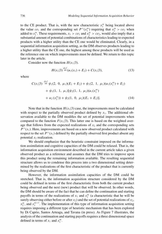
However, the information assimilation capacities of the DM could bestretched. That is, the information acquisition structure considered by the DMcould be defined in terms of the first characteristic from both the current productbeing observed and the next (new) product that will be observed. In other words,the DM should be aware of the fact that he can define the continuation and startingpayoffs in terms of the realizations of x1 and xm1 (a characteristic that he will besurely observing either before or after x2) and the set of potential realizations of x2,xm2 , and xm+1
1 . The implementation of this type of information acquisition settingrequires imposing a different type of heuristic mechanism that has been exploredby Di Caprio, Santos Arteaga, and Tavana (in press). As Figure 7 illustrates, theanalysis of the continuation and starting payoffs requires a three dimensional spacedefined in terms of x1 and xm1 .
Tavana, Di Caprio, and Arteaga 737
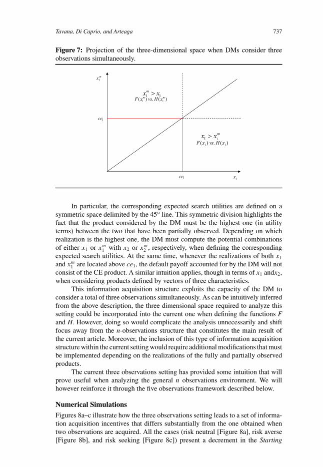
Figure 7: Projection of the three-dimensional space when DMs consider threeobservations simultaneously.
1ce
mx1
1x
11 xxm > )(.)( 11
mm xHvsxF
1ce
mxx 11 > )(.)( 11 xHvsxF
In particular, the corresponding expected search utilities are defined on asymmetric space delimited by the 45° line. This symmetric division highlights thefact that the product considered by the DM must be the highest one (in utilityterms) between the two that have been partially observed. Depending on whichrealization is the highest one, the DM must compute the potential combinationsof either x1 or xm1 with x2 or xm2 , respectively, when defining the correspondingexpected search utilities. At the same time, whenever the realizations of both x1
and xm1 are located above ce1, the default payoff accounted for by the DM will notconsist of the CE product. A similar intuition applies, though in terms of x1 andx2,when considering products defined by vectors of three characteristics.
This information acquisition structure exploits the capacity of the DM toconsider a total of three observations simultaneously. As can be intuitively inferredfrom the above description, the three dimensional space required to analyze thissetting could be incorporated into the current one when defining the functions Fand H. However, doing so would complicate the analysis unnecessarily and shiftfocus away from the n-observations structure that constitutes the main result ofthe current article. Moreover, the inclusion of this type of information acquisitionstructure within the current setting would require additional modifications that mustbe implemented depending on the realizations of the fully and partially observedproducts.
The current three observations setting has provided some intuition that willprove useful when analyzing the general n observations environment. We willhowever reinforce it through the five observations framework described below.
Numerical Simulations
Figures 8a–c illustrate how the three observations setting leads to a set of informa-tion acquisition incentives that differs substantially from the one obtained whentwo observations are acquired. All the cases (risk neutral [Figure 8a], risk averse[Figure 8b], and risk seeking [Figure 8c]) present a decrement in the Starting

738 Modeling Sequential Information Acquisition Behavior
Figure 8: Information acquisition incentives with three observations.
dominance pattern obtained within the two observations environment. The Start-ing option still dominates the Continuing one through most of the domain X1 butto a much lesser extent than in the two observations case.
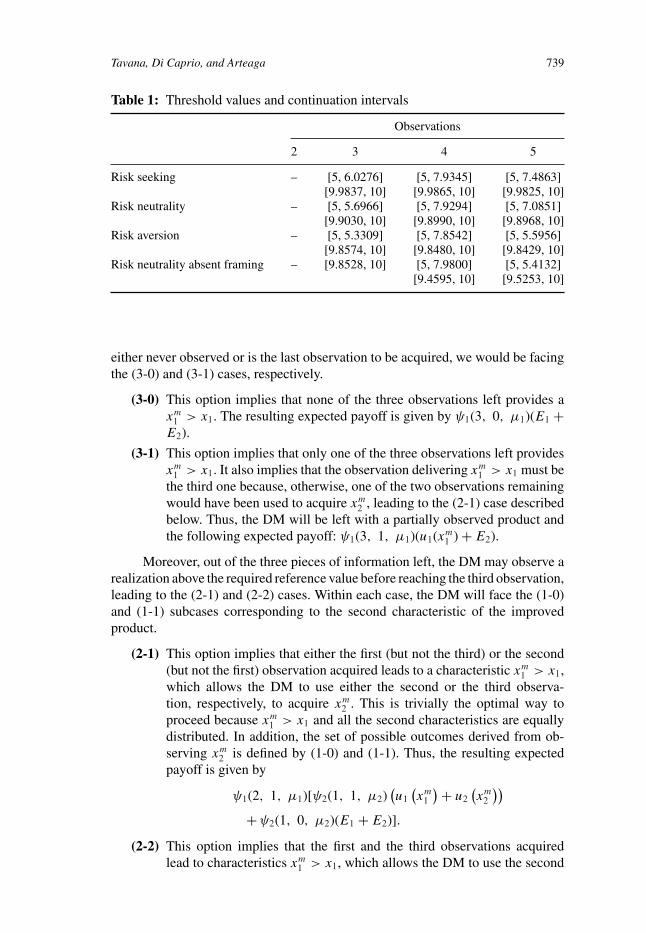
Thus, when having a third observation to acquire, DMs will favor the ac-quisition of information on a new product over continuing with the one initiallyobserved. At the same time, note how the dominant tendency extends over a widerinterval in the risk averse case, followed by the risk neutral and the risk seekingone, respectively. The exact interval values are presented in Table 1.
Finally, as will become explicit in the setting with five observations, we haveassumed the DM to account for the possibility of selecting the best product amongthe potentially acceptable ones expected to be observed.
The Proposed Information Acquisition Structure with Five Observations
Similarly to the three observations case, when calculating the function F (x1|5) wemust consider the following set of combinations based on the three observationsthat remain to be acquired after gathering two observations on the first product:(3-0), (3-1), (2-1), and (2-2). If the realization required (to be higher than x1) is
Tavana, Di Caprio, and Arteaga 739
Table 1: Threshold values and continuation intervals
Observations
2 3 4 5
Risk seeking – [5, 6.0276] [5, 7.9345] [5, 7.4863][9.9837, 10] [9.9865, 10] [9.9825, 10]
Risk neutrality – [5, 5.6966] [5, 7.9294] [5, 7.0851][9.9030, 10] [9.8990, 10] [9.8968, 10]
Risk aversion – [5, 5.3309] [5, 7.8542] [5, 5.5956][9.8574, 10] [9.8480, 10] [9.8429, 10]
Risk neutrality absent framing – [9.8528, 10] [5, 7.9800] [5, 5.4132][9.4595, 10] [9.5253, 10]
either never observed or is the last observation to be acquired, we would be facingthe (3-0) and (3-1) cases, respectively.
(3-0) This option implies that none of the three observations left provides axm1 > x1. The resulting expected payoff is given by ψ1(3, 0, μ1)(E1 +E2).
(3-1) This option implies that only one of the three observations left providesxm1 > x1. It also implies that the observation delivering xm1 > x1 must bethe third one because, otherwise, one of the two observations remainingwould have been used to acquire xm2 , leading to the (2-1) case describedbelow. Thus, the DM will be left with a partially observed product andthe following expected payoff: ψ1(3, 1, μ1)(u1(xm1 ) + E2).
Moreover, out of the three pieces of information left, the DM may observe arealization above the required reference value before reaching the third observation,leading to the (2-1) and (2-2) cases. Within each case, the DM will face the (1-0)and (1-1) subcases corresponding to the second characteristic of the improvedproduct.
(2-1) This option implies that either the first (but not the third) or the second(but not the first) observation acquired leads to a characteristic xm1 > x1,which allows the DM to use either the second or the third observa-tion, respectively, to acquire xm2 . This is trivially the optimal way toproceed because xm1 > x1 and all the second characteristics are equallydistributed. In addition, the set of possible outcomes derived from ob-serving xm2 is defined by (1-0) and (1-1). Thus, the resulting expectedpayoff is given by
ψ1(2, 1, μ1)[ψ2(1, 1, μ2)(u1(xm1)+ u2
(xm2))
+ψ2(1, 0, μ2)(E1 + E2)].
(2-2) This option implies that the first and the third observations acquiredlead to characteristics xm1 > x1, which allows the DM to use the second
740 Modeling Sequential Information Acquisition Behavior
observation to acquire xm2 , that is, the second characteristic from thesecond product observed, while a third product with xm+1
1 > x1 remainspartially observed, its second characteristic defined by the CE value.Due to the partial observation of the third and final product, the set ofpotential outcomes derived from observing xm2 is given by (1-0) and(1-1). Therefore, the corresponding expected payoff is given by
ψ1(2, 2, μ1)[ψ2(1, 1, μ2) max
{(u1(xm1 ) + u2(xm2 )),
(u1(xm+1
1
)+ E2)}
+ψ2(1, 0, μ2)(u1(xm+1
1
)+ E2) ].
Note that the two possibilities regarding the potential realizations of xm2 mustbe accounted for separately. That is, ψ2(1, 1, μ2) implies that the realization ofxm2 delivers an observation located within P+(x1), leading to an expected payoffdefined by the fully observed new product m and the partially observed newproduct m+ 1. Both these products are the result of the search process and theDM must choose the product providing the highest (expected) utility. Similarly,the probability ψ2(1, 0, μ2) indicates that xm2 does not deliver a product locatedwithin P+(x1) and the DM is therefore left with the partially observed productm+ 1.
Consider now the four remaining observations that define the functionH (x1|5). As already explained in the previous subsection, the DM has an ex-tra unit of information available to acquire in this setting relative to the F (x1|5)one. The DM has to account for the following set of potential outcomes: (4-0),(4-1), (3-1), (3-2), and (2-2). If the realization required (to be higher than x1) iseither never observed or is the last observation to be acquired, we would be facingthe (4-0) and (4-1) cases, respectively.
(4-0) This option implies that none of the four observations left provides axm1 > x1. The resulting expected payoff is given by ψ1(4, 0, μ1)(E1 +E2).
(4-1) This option implies that only one of the four observations left providesa xm1 > x1. It also implies that the observation providing a xm1 > x1
must be the fourth one. Otherwise, any of the other three observationsavailable would have been used to acquire xm2 , leading to the (3-1)subcase described below. In other words, if the observation deliveringxm1 > x1 was not the last one but, for example, the third one, the lastobservation available would have been used to acquire information onxm2 , an event described by the (3-1) subcase. Thus, in the (4-1) case theDM observes a partially improved product, leading to an expected payoffgiven by: ψ1(4, 1, μ1)(u1(xm1 ) + E2).
Moreover, out of the four pieces of information left, the DM may observeonly one realization above the required reference value before reaching the fourthobservation, leading to the (3-1) case. Within this case, the DM will face the (1-0)and (1-1) subcases corresponding to the second characteristic of the improvedproduct.
(3-1) This option implies that only one of the first three observationsprovides a xm1 > x1, which allows the DM to use one of the remaining
Tavana, Di Caprio, and Arteaga 741
observations to acquire xm2 , that is, the second characteristic fromthe new observed product. Clearly, the set of possible outcomesderived from observing xm2 is defined by (1-0) and (1-1). The corre-sponding expected payoff must therefore be based on combinationsof xm1 and xm2 leading to products located above the referenceone (x1, P
+(x1)): ψ1(3, 1, μ1)[ψ2(1, 1, μ2)(u1(xm1 ) + u2(xm2 ))+ψ2(1, 0, μ2)(E1 + E2)].
Finally, out of the four pieces of information left, the DM may observe tworealizations located above the required reference value, leading to the (3-2) and(2-2) cases. Within each case, the DM will face different subcases correspondingto the second characteristic of the improved product(s).
(3-2) This option implies that either the first and the fourth or the second andthe fourth observations lead to a characteristic xm1 > x1, which allowsthe DM to use one of the remaining observations (the second or the thirdone, respectively) to acquire xm2 , that is, the second characteristic fromthe new observed product, while a second new product with xm+1
1 > x1
remains partially observed, its second characteristic defined by the CEvalue. As in the previous subcase, the set of possible outcomes derivedfrom observing xm2 is defined by (1-0) and (1-1). The resulting expectedpayoff is therefore given by
ψ1(3, 2, μ1)[ψ2(1, 1, μ2) max
{(u1(xm1)+ u2
(xm2)),(
u1(xm+1
1
)+ E2)}+ ψ2(1, 0, μ2)(u1(xm+1
1 ) + E2)].
(2-2) This option implies that the first and the third observations acquired leadto a characteristic xm1 > x1, which allows the DM to use the second andfourth observations to acquire xm2 and xm+1
2 , respectively, that is, thesecond characteristic from the first and second new observed products.Similarly to the previous subcases, the set of possible outcomes derivedfrom observing xm2 and xm+1
2 is defined by (2-0), (2-1), and (2-2). Thecorresponding expected payoff is given by
ψ1(2, 2, μ1)[ψ2(2, 2, μ2) max{(u1(xm1 ) + u2(xm2 )),
(u1(xm+11 ) + u2(xm+1
2 ))} + ψ2(2, 1, μ2)(u1(xm1 ) + u2(xm2 ))+ψ2(2, 0, μ2)(E1 + E2)].
Note that the DM must account for the three potential search outcomesseparately. First, ψ2(2, 2, μ2) implies that both observations xm2 and xm+1
2 deliverrealizations located within P+(x1), leading to an expected payoff defined by thenew products, m and m+ 1, being fully observed. These products are the resultof the search process and the DM must choose the one providing the highestutility. Second, ψ2(2, 1, μ2) implies that only one of the observations xm2 andxm+1
2 delivers a realization located within P+(x1), leading to an expected payoffdefined by either the new productm or the new productm+ 1 being fully observed.Without loss of generality, we have used them notation to refer to the fully observedproduct. Finally,ψ2(2, 0, μ2) indicates that none of the second observations from
742 Modeling Sequential Information Acquisition Behavior
the new products delivers a realization located within P+(x1) and the DM istherefore left with the random CE outcome.
We are now able to write an expression for the functionsF (x1|5) andH (x1|5).The former reads as follows:
F (x1|5)def=
∫P+(x1)
μ2(x2) (u1(x1) + u2(x2)) dx2 + A(x1|5)
+∫
P−(x1)
μ2(x2) (E1 + E2) dx2 + B(x1|5), (15)
where
A(x1|5)def=
∫P+(x1)
μ2(x2)[ψ1(3, 0, μ1)(E1 + E2) + ψ1(3, 1, μ1)(u1(xm1 ) + E2)
+ ψ1(2, 1, μ1)[ψ2(1, 1, μ2)(u1(xm1 ) + u2(xm2 )) + ψ2(1, 0, μ2)(E1 + E2)]
+ ψ1(2, 2, μ1)[ψ2(1, 1, μ2) max{(u1(xm1 ) + u2(xm2 )), (u1(xm+11 ) + E2)}
+ ψ2(1, 0, μ2)(u1(xm+11 ) + E2)]]dx2, (16)
B(x1|5)def=
∫P−(x1)
μ2(x2)[ψ1(3, 0, μ1)(E1 + E2) + ψ1(3, 1, μ1)(u1(xm1 ) + E2)
+ ψ1(2, 1, μ1)[ψ2(1, 1, μ2)(u1(xm1 ) + u2(xm2 )) + ψ2(1, 0, μ2)(E1 + E2)]
+ ψ1(2, 2, μ1)[ψ2(1, 1, μ2) max{(u1(xm1 ) + u2(xm2 )), (u1(xm+11 ) + E2)}
+ ψ2(1, 0, μ2)(u1(xm+11 ) + E2)]]dx2. (17)
Note that the integration sets, P+(x1) and P−(x1), depend on the initialobservation acquired, which defines the (expected) product that must be improvedupon through the information acquisition process. In the function F case, potentialimprovements of the second characteristic are defined with respect to P+(x1). Ifwe were to use P+(xm1 ), with xm1 > x1, then some acceptable characteristics ofX2 would be lower than those defined within P+(x1). However, we are assumingthrough this section that DMs only consider full potential improvements relativeto the reference (partially observed) product given by (x1, P
+(x1)). As a result,xm1 must be located above x1 and xm2 must be potentially at least as good asx2 ∈ P+(x1). Defining improvements on the function H (x1|5) is subject to thesame type of [subjective] constraint.
H (x1|5)def= (u1(x1) + E2) + C(x1|5) (18)
Tavana, Di Caprio, and Arteaga 743
with
C(x1|5)def= ψ1(4, 0, μ1)(E1 + E2) + ψ1(4, 1, μ1)(u1(xm1 ) + E2)
+ ψ1(3, 1, μ1)[ψ2(1, 1, μ2)(u1(xm1 ) + u2(xm2 )) + ψ2(1, 0, μ2)(E1 + E2)]
+ ψ1(3, 2, μ1)[ψ2(1, 1, μ2) max{(u1(xm1 ) + u2(xm2 )), (u1(xm+11 ) + E2)}
+ ψ2(1, 0, μ2)(u1(xm+11 ) + E2)]
+ ψ1(2, 2, μ1)[ψ2(2, 2, μ2) max{(u1(xm1 ) + u2(xm2 )), (u1(xm+11 )+u2(xm+1
2 ))}
+ ψ2(2, 1, μ2)(u1(xm1 ) + u2(xm2 )) + ψ2(2, 0, μ2)(E1 + E2)]. (19)
The improvements in the functionH case are clearly based on the x1 realiza-tion acquired, which defines the partially observed product that must be improvedupon. In this regard, the reference value determining the product to improve isgiven by P+(x1). However, we may also assume that the set of potential improve-ments is determined either by 〈ce1, ce2〉, whenever x1 ≤ ce1, or by 〈x1, ce2〉,whenever x1 > ce1. In this case, the new product must improve upon both, theobserved variable and the expected utility from the unobserved one. We considerthis possibility in “Framing and Reference Products” section.
Numerical Simulations
When computing the functions F (x1|5) andH (x1|5) numerically, we have made adistinction among the expected utility levels that may be achieved from differentpotential final choice sets such as, for example,
max{(u1(xm1 ) + u2(xm2 )), (u1(xm+11 ) + u2(xm+1
2 ))};max{(u1(xm1 ) + u2(xm2 )), (u1(xm+1
1 ) + E2)};(u1(xm1 ) + u2(xm2 )).
(20)
The DM does not know the exact products that he will be observing, justthe intervals containing them and the number of improved products he will get toobserve. Clearly, observing ten products from the intervals (x1, β1) and P+(x1)should provide a different expected payoff from observing only one product. Inother words, the probability of obtaining a better product from a given subsetshould increase in the number of products observed, with the DM subjectivelyaccounting for this fact when computing his expected search payoffs. While theconsumer psychology literature has extensively analyzed the effects of optimismand pessimism on expectations (Kahneman & Tversky, 2000), we opt for a rela-tively simple rule to determine the expected utility obtained when several productscontained within the intervals (x1, β1) and P+(x1) are observed.
For example, given xm1 > x1 and xm2 ∈ P+(x1), assume that each Xk , k =1, 2 is uniformly distributed on its domain [αk, βk]. We have applied the followingrule when calculating the expected utility obtained by the DM after observing n
744 Modeling Sequential Information Acquisition Behavior
products within the intervals (x1, β1) and P+(x1):
β1+x1
2∫x1
(1 − n−1
100
β1 − x1
)u1(xm1 )dxm1 +
β1∫β1+x1
2
⎛⎜⎝1 + n− 1
100β1 − x1
⎞⎟⎠ u1(xm1 )dxm1
+
u−12 (u2(β2)+E1+E2−u1(x1))
2∫u−1
2 (E1+E2−u1(x1))
(1 − n−1
100
β2 − u−12 (E1 + E2 − u1(x1))
)u2(xm2 )dxm2
+β2∫
u−12 (u2(β2)+E1+E2−u1(x1))
2
(1 + n−1
100
β2 − u−12 (E1 + E2 − u1(x1))
)u2(xm2 )dxm2 .(21)
That is, after expecting to observe n products providing a higher utility thanthe initial [reference] one, we have assumed that the DM shifts probability massfrom the lower half of the uniform distribution to the upper one at a rate of 1
100 .Here n accounts for the number of fully observed products providing a higherexpected utility than the reference [initially observed] one. In other words, if theDM expects to fully observe one product better than the reference one, then n = 1;if he expects to fully observe one product and another one partially, then n = 1.5,that is, a partially observed product adds 0.5 to the probability shift, while expectingto fully observe two products leads to n = 2. We have assumed that after expectingto fully observe n = 101 products, the DM shifts the whole mass from the lowerhalf of the uniform distribution defined by x1 to the upper one.
Clearly, the expected improvement defined on the first characteristic is muchsimpler to compute than the improvement on the second one, because the shapeof the utility function determines the lower limit point defining the set P+(x1).Thus, as intuition suggests, risk taking, risk neutral and risk averse DMs will havedifferent information acquisition incentives and behavior. Note that the functionalform assumed above generates a relatively small distortion on the expected utilityderived from the set of potential improved products. In this regard, DMs could beassumed to be either more optimistic or pessimistic or completely unaware of thisadjustment.
Figures 9a–c illustrate the risk neutral, risk averse and risk seeking environ-ments, respectively, when four observations are acquired by the DMs. Similarly,Figures 10a–c account for these respective environments within the five obser-vations setting. The diversity of scenarios obtained is considerable, with all thesettings being almost identical in information acquisition incentives when fourobservations are considered, while differing significantly in the five observationscase, see the corresponding entries in Table 1.
We should highlight the decrease in the width of the continuation intervalsas we move from a risk seeking environment towards a risk averse one. That is,risk seekers are more prone to continue acquiring information on the product being
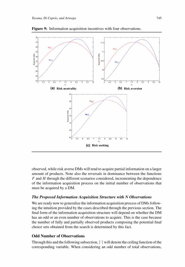
Tavana, Di Caprio, and Arteaga 745
Figure 9: Information acquisition incentives with four observations.
observed, while risk averse DMs will tend to acquire partial information on a largeramount of products. Note also the reversals in dominance between the functionsF andH through the different scenarios considered, incrementing the dependenceof the information acquisition process on the initial number of observations thatmust be acquired by a DM.
The Proposed Information Acquisition Structure with N Observations
We are ready now to generalize the information acquisition process of DMs follow-ing the intuition provided by the cases described through the previous section. Thefinal form of the information acquisition structure will depend on whether the DMhas an odd or an even number of observations to acquire. This is the case becausethe number of fully and partially observed products composing the potential finalchoice sets obtained from the search is determined by this fact.
Odd Number of Observations
Through this and the following subsection, �·� will denote the ceiling function of thecorresponding variable. When considering an odd number of total observations,

746 Modeling Sequential Information Acquisition Behavior
Figure 10: Information acquisition incentives with five observations.
as in the cases described through the previous section, we have the followingexpressions for the functions F and H .
Function F
The total that must be considered by the DM equals �n−12 �, with n consisting of
the total number of observations that will be gathered by the DM. In this case, theDM must account for the acquisition of the remaining n− 2 observations (i.e., 9in the case with a total of 11, 3 in the case with a total of 4) following the patterndescribed below for the potential combinations (n− j -j − 2), (n− j -j − 1),where j = 2, . . . , �n2 �.∫P+(x1)
μ2(x2)[ψ1(n− j, j − 2, μ1(xm1 > x1))
[ψ2(j − 2, 0, μ2(xm2 ∈ P+(x1)))(E1 + E2)
+
Tavana, Di Caprio, and Arteaga 747
ψ2(j − 2, 1, μ2(xm2 ∈ P+(x1)))(u1(xm1 ) + u2(xm2 ))
+ψ2(j − 2, 2, μ2(xm2 ∈ P+(x1)))
max{(u1(xm1 ) + u2(xm2 )), (u1(xm+11 ) + u2(xm+1
2 ))}+ · · · +ψ2(j − 2, j − 2, μ2(xm2 ∈ P+(x1)))
max{(u1(xm1 ) + u2(xm2 )), . . . , (u1(xm+j−31 ) + u2(xm+j−3
2 ))}]]dx2, (22)
+∫P+(x1)
μ2(x2)[ψ1(n− j, j − 1, μ1(xm1 > x1))
[ψ2(j − 2, 0, μ2(xm2 ∈ P+(x1)))(u1(xm+j−21 ) + E2)
+ψ2(j − 2, 1, μ2(xm2 ∈ P+(x1))) max{(u1(xm1 ) + u2(xm2 )), (u1(xm+j−2
1 ) + E2)}+
ψ2(j − 2, 2, μ2(xm2 ∈ P+(x1)))
max{(u1(xm1 ) + u2(xm2 )), (u1(xm+11 ) + u2(xm+1
2 )), (u1(xm+j−21 ) + E2)}
+ · · · +ψ2(j − 2, j − 2, μ2(xm2 ∈ P+(x1))) max(u1(xm1 ){u2(xm2 ))
, . . . , (u1(xm+j−31 ) + u2(xm+j−3
2 )), (u1(xm+j−21 ) + E2)}]]dx2. (23)
Note that we have only considered the section of the function F definedwithin the set P+(x1), because the complementary section based on P−(x1) hasthe same structure. The notation and intuition describing the function follow fromthe ones used to describe the scenarios with three and five observations. The maindifference arising in the general case is the division of the function in two separateblocks, which follows from the potential combinations of fully and partially ob-served products located above the reference one. A similar description applies tothe function H , whose extra observation leads to a third block of potential combi-nations having to be considered. Clearly, the above blocks compose part A(x1|n)of the function F (x1|n), while the three blocks introduced below compose partC(x1|n) of the function H (x1|n).
Function H
The total number of combinations that must be considered by the DM equals �n2 �,with n consisting of the total number of observations that will be gathered by the
748 Modeling Sequential Information Acquisition Behavior
DM. The DM must account for the acquisition of the remaining n− 1 observations(i.e., 10 in the case with a total of 11, 4 in the case with a total of 5) following thepattern described below for the potential combinations (n− j -j − 1), (n− j - j ),where j = 1, ..., �n2 � − 1.
ψ1(n− j, j − 1, μ1(xm1 > x1))
[ψ2(j − 1, 0, μ2(xm2 ∈ P+(x1)))(E1 + E2)
+ ψ2(j − 1, 1, μ2(xm2 ∈ P+(x1)))(u1(xm1 ) + u2(xm2 ))
+ ψ2(j − 1, 2, μ2(xm2 ∈ P+(x1)))
max{(u1(xm1 ) + u2(xm2 )), (u1(xm+11 ) + u2(xm+1
2 ))}+ ...+ ψ2(j − 1, j − 1, μ2(xm2 ∈ P+(x1)))
max{(u1(xm1 ) + u2(xm2 )), ..., (u1(xm+j−21 ) + u2(xm+j−2
2 ))}]+
(24)
ψ1(n− j, j, μ1(xm1 > x1))
[ψ2(j − 1, 0, μ2(xm2 ∈ P+(x1)))(u1(xm+j−11 ) + E2)
+ ψ2(j − 1, 1, μ2(xm2 ∈ P+(x1))) max{(u1(xm1 ) + u2(xm2 )), (u1(xm+j−11 ) + E2)}
+ ψ2(j − 1, 2, μ2(xm2 ∈ P+(x1)))
max{(u1(xm1 ) + u2(xm2 )), (u1(xm+11 ) + u2(xm+1
2 )), (u1(xm+j−11 ) + E2)}
+...+ ψ2(j − 1, j − 1, μ2(xm2 ∈ P+(x1)))max{(u1(xm1 ) + u2(xm2 )), ..., (u1(xm+j−2
1 ) + u2(xm+j−22 )), (u1(xm+j−1
1 ) + E2)}]+
(25)
ψ1(n− ⌈
n2
⌉,⌈n2
⌉− 1, μ1(xm1 > x1))
[ψ2(⌈
n2
⌉− 1, 0, μ2(xm2 ∈ P+(x1)))
(E1 + E2)
+ ψ2(⌈
n2
⌉− 1, 1, μ2(xm2 ∈ P+(x1)))
(u1(xm1 ) + u2(xm2 ))
+ ψ2(⌈
n2
⌉− 1, 2, μ2(xm2 ∈ P+(x1)))
max{(u1(xm1 ) + u2(xm2 )),
(u1(xm+11 ) + u2(xm+1
2 ))} + ...+ ψ2(⌈
n2
⌉− 1,⌈n2
⌉− 1, μ2(xm2 ∈ P+(x1)))
max{(u1(xm1 ) + u2(xm2 )), ..., (u1(xm+
⌈n2
⌉−2
1 ) + u2(xm+
⌈n2
⌉−2
2 ))}].
(26)
As in the function F case, the division of the function H in three separateblocks follows from the potential combinations of fully and partially observedproducts located above the initial reference one.
Even Number of Observations
Consider now an even number of total observations. For illustrative purposes,assume that the DM may acquire a total of four or six observations. The followingcombinations, leading to the corresponding expressions for F and H , must beaccounted for.
The potential combinations faced by the DM when computing the functionFin the setting with four observations are (2-0), (2-1), and (1-1), while the functionHrequires (3-0), (3-1), (2-1), and (2-2). Similarly, in the setting with six observations,the potential combinations faced by the DM when computing the function F are(4-0), (4-1), (3-1), (3-2), and (2-2), while the function H requires (5-0), (5-1),(4-1), (4-2), (3-2), and (3-3). The intuition in all these cases is identical to the

Tavana, Di Caprio, and Arteaga 749
one employed to describe the environments with an odd number of observations.However, in the current setting, the function F will be the one composed by threedifferent blocks, while H remains composed by only two.
In order to simplify the presentation, we will only describe theψ2(·, 0, μ2(xm2 ∈ P+(x1))) and ψ2(·, ·, μ2(xm2 ∈ P+(x1))) potential out-comes, because the remaining ones can be easily inferred from the context.Moreover, we have already provided additional potential outcomes for eachblock composing the functions F and H when describing the odd number ofobservations environment above.
Function F
The total number of combinations that must be considered by the DM equals �n2 �,with n consisting of the total number of observations that will be gathered by theDM. In this case, the DM must account for the acquisition of the remaining n− 2observations (i.e., 8 in the case with a total of 10, 4 in the case with a total of6) following the pattern described below for the potential combinations (n− j -j − 2), (n− j - j − 1), where j = 2, ..., � n+1
2 � − 1.∫P+(x1)
μ2(x2)[ψ1(n− j, j − 2, μ1(xm1 > x1))
[ψ2(j − 2, 0, μ2(xm2 ∈ P+(x1)))(E1 + E2)++...+ ψ2(j − 2, j − 2, μ2(xm2 ∈ P+(x1)))
max{(u1(xm1 ) + u2(xm2 )), ..., (u1(xm+j−31 ) + u2(xm+j−3
2 ))}]]dx2+
(27)
∫P+(x1)
μ2(x2)[ψ1(n− j, j − 1, μ1(xm1 > x1))
[ψ2(j − 2, 0, μ2(xm2 ∈ P+(x1)))(u1(xm+j−21 ) + E2)
+...+ ψ2(j − 2, j − 2, μ2(xm2 ∈ P+(x1)))
max{(u1(xm1 ) + u2(xm2 )), ..., (u1(xm+j−31 ) + u2(xm+j−3
2 )), (u1(xm+j−21 ) + E2)}]]dx2+
(28)
∫P+(x1)
μ2(x2)[ψ1
(n−
⌈n+ 1
2
⌉,⌈n
2
⌉− 1, μ1(xm1 > x1)
)
[ψ2
(⌈n2
⌉− 1, 0, μ2(xm2 ∈ P+(x1))
)(E1 + E2)
+...+ ψ2
(⌈n2
⌉− 1,
⌈n2
⌉− 1, μ2(xm2 ∈ P+(x1))
)max{(u1(xm1 ) + u2(xm2 )), ..., (u1(x
m+⌈n2
⌉−2
1 ) + u2(xm+
⌈n2
⌉−2
2 ))}]]dx2.
(29)
Function H
The total number of combinations that must be considered by the DM equals �n2 �,with n consisting of the total number of observations that will be gathered by theDM. In this case, the DM must account for the acquisition of the remaining n− 1observations (i.e., 9 in the case with a total of 10, 5 in the case with a total of
750 Modeling Sequential Information Acquisition Behavior
6) following the pattern described below for the potential combinations (n− j -j − 1), (n− j - j ), where j = 1, ..., � n2 �.
ψ1(n− j, j − 1, μ1(xm1 > x1))
[ψ2(j − 1, 0, μ2(xm2 ∈ P+(x1)))(E1 + E2)
+...+ ψ2(j − 1, j − 1, μ2(xm2 ∈ P+(x1)))
max{(u1(xm1 ) + u2(xm2 )), ..., (u1(xm+j−21 ) + u2(xm+j−2
2 ))}]+
(30)
ψ1(n− j, j, μ1(xm1 > x1))
[ψ2(j − 1, 0, μ2(xm2 ∈ P+(x1)))(u1(xm+j−11 ) + E2)
+...+ ψ2(j − 1, j − 1, μ2(xm2 ∈ P+(x1)))
max{(u1(xm1 ) + u2(xm2 )), ..., (u1(xm+j−21 ) + u2(xm+j−2
2 )), (u1(xm+j−11 ) + E2)}].
(31)
FRAMING AND REFERENCE PRODUCTS
Until now, the set of potential improvements upon the reference realization hasbeen defined with respect to the pair (x1, P
+(x1)). This assumption can be justifiedas follows. First, it accounts for any framing effect that may result from the(partial) observation of the initial product. Second, it conditions improvements onthe information available to the DM, who does not know the outcome from thesecond observation but is able to compute the set of acceptable realizations. In thisregard, all potential improvements are consistently based on the first characteristicobserved, x1, even those defining section B within the corresponding function F.We refer to this scenario as the framing environment. It assumes that initial andrealized observations condition the information acquisition behavior of the DM bydefining the set of acceptable expected ones.
We can however redefine this environment by modifying the acceptancerequirements of DMs regarding the expectations relative to the first and secondcharacteristics whenever x1 ≤ ce1. That is, acceptable improvements could bedefined relative to the pair of expected values 〈ce1, ce2〉. This would clearlymodify the information acquisition incentives of DMs. In this case, two typesof improvement would be required on the initial product before having actuallyobserved it fully. If x1 > ce1, we will assume that the DM considers the referencepair (x1, P
+(x1)). However, if x1 ≤ ce1, then the DM would shift his referencerequirements to the pair 〈ce1, ce2〉, due to the absence of an acceptable observedproduct.
The framing approach focuses on the potential improvements derived fromthe information acquisition process while the elimination of framing shifts the focusof the search process to the set of acceptable products expected to be obtained.Though relatively small, the effect of framing [or its absence] is noticeable on theinformation acquisition behavior of DMs even when only three observations areacquired. However, its main consequences are better understood when using, as abasic example, an explicit formulation of this setting, which is described by the
Tavana, Di Caprio, and Arteaga 751
following set of equations:
F (x1|3)def=
∫P+(x1)
μ2(x2) (u1(x1) + u2(x2)) dx2 + A(x1|3)
+∫
P−(x1)
μ2(x2) (E1 + E2) dx2 + B(x1|3), (32)
A(x1|3)def=
∫P+(x1)
μ2(x2)[ψ1(1, 0, μ1(xm1 > x1))(E1 + E2)
+ ψ1(1, 1, μ1(xm1 > x1))(u1(xm1 ) + E2)]dx2, (33)
B(x1|3)def=
∫P−(x1)
μ2(x2)[ψ1(1, 0, μ1(xm1 > x1))(E1 + E2)
+ ψ1(1, 1, μ1(xm1 > x1))(u1(xm1 ) + E2)]dx2. (34)
Note how we have emphasized explicitly withinμ1(·) that the reference pointconsidered by the DM when defining potential improvements is given by x1. Thisreference choice constitutes the framing effect that determines improvements withrespect to the pair (x1, P
+(x1)). Clearly, part A remains unaffected by the fram-ing effect, as expected improvements are defined on the fully observed productsproviding a higher utility than the CE one. However, the framing effect becomesevident within part B, which allows for potential improvements over x1, the initialobservation serving as a reference point, even if they deliver products that willnot be chosen by the DM. To see why this is the case, consider the alternativesetting without framing, where the DM accounts explicitly for the realization ofthe second characteristic (whether either about to be actually observed, as in Aand B, or expected, as in C) when determining his optimal information acquisitionstrategy
F (x1|3)def=
∫P+(x1)
μ2(x2) (u1(x1) + u2(x2)) dx2 + A(x1|3)
+∫
P−(x1)
μ2(x2) (E1 + E2) dx2 + B(x1|3), (35)
A(x1|3)def=
∫P+(x1)
μ2(x2)[ψ1(1, 0, μ1(xm1 > x1))(E1 + E2)
+ ψ1(1, 1, μ1(xm1 > x1))(u1(xm1 ) + E2)]dx2,
(36)
752 Modeling Sequential Information Acquisition Behavior
B(x1|3)def=
∫P−(x1)
μ2(x2)[ψ1(1, 0, μ1(xm1 > ce1))(E1 + E2)
+ ψ1(1, 1, μ1(xm1 > ce1))(u1(xm1 ) + E2)]dx2.
(37)
Note the immediate change in part B, where the reference point has beenshifted within μ1(·) to the ce1-based product. That is, after the fully observedinitial product delivers a utility below the CE one, the DM has to start acquiringinformation without a reference product to improve upon. As a result, the DMis assumed to use the coordinates of the CE product, that is, 〈ce1, ce2〉, as thecorresponding reference values.
Thus, the new first characteristic xm1 must be located above the value ce1
and the corresponding set P+(xm1 ) should require that xm2 > ce2. These differencesbecome much more evident when analyzing part C within function H . The fram-ing environment considers the product partially observed as the main referencepoint defining the improvements expected to be obtained from the informationacquisition process.
H (x1|3)def= (u1(x1) + E2) + C(x1|3), (38)
C(x1|3)def= ψ1(2, 0, μ1(xm1 > x1))(E1 + E2) + ψ1(2, 1, μ1(xm1 > x1))(u1(xm1 ) + E2)
+ ψ1(1, 1, μ1(xm1 > x1))[ψ2(1, 1, μ2(xm2 ∈ P+(x1)))(u1(xm1 ) + u2(xm2 ))
+ ψ2(1, 0, μ2(xm2 ∈ P+(x1)))(E1 + E2)].
(39)
When eliminating the framing effect, part C must be divided in two differ-entiated subcases. The first one is defined for x1 ∈ [α1, ce1]. Observing an initialrealization within this interval implies that xm1 must improve upon the value ce1
and xm2 should be based on the corresponding potential realizations that improveupon ce2, that is, μ2(xm2 ∈ P+(xm1 )|xm2 > ce2).
C(x1|3)def= ψ1(2, 0, μ1(xm1 > ce1))(E1 + E2) + ψ1(2, 1, μ1(xm1 > ce1))(u1(xm1 ) + E2)
+ ψ1(1, 1, μ1(xm1 > ce1))[ψ2(1, 1, μ2(xm2 ∈ P+(xm1 )|xm2 > ce2))
×(u1(xm1 ) + u2(xm2 )) + ψ2(1, 0, μ2(xm2 ∈ P+(xm1 )|xm2 > ce2))
×(E1 + E2)]. (40)
Note that both xm1 and xm2 must constitute improvements upon the CE ref-erence product defined by ce1 and ce2, respectively. This required improvementis based on the fact that the initial product observed, (x1 ≤ ce1, E2), does notprovide a higher utility than the CE one.
The second subcase is defined for x1 ∈ [ce1, β1], which implies that xm1must improve upon the initial value x1 and xm2 should be based on the correspond-ing potential realizations improving upon the CE product while constrained byμ2(xm2 ∈ P+(x1)|xm2 > ce2). That is, because x2 remains unobserved through H ,though it is expected to be observed when defining F , the resulting reference valuewill be given by ce2. In other words, potential improvements are defined withrespect to the initial product observed, which is given by the first characteristic
Tavana, Di Caprio, and Arteaga 753
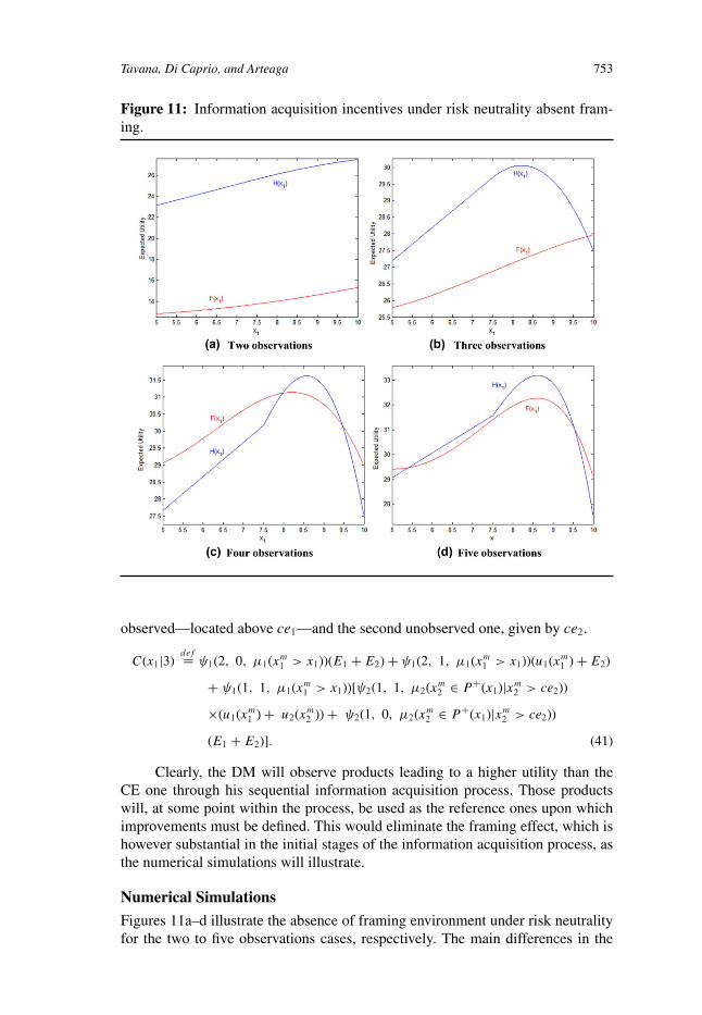
Figure 11: Information acquisition incentives under risk neutrality absent fram-ing.
observed—located above ce1—and the second unobserved one, given by ce2.
C(x1|3)def= ψ1(2, 0, μ1(xm1 > x1))(E1 + E2) + ψ1(2, 1, μ1(xm1 > x1))(u1(xm1 ) + E2)
+ ψ1(1, 1, μ1(xm1 > x1))[ψ2(1, 1, μ2(xm2 ∈ P+(x1)|xm2 > ce2))
×(u1(xm1 ) + u2(xm2 )) + ψ2(1, 0, μ2(xm2 ∈ P+(x1)|xm2 > ce2))
(E1 + E2)]. (41)
Clearly, the DM will observe products leading to a higher utility than theCE one through his sequential information acquisition process. Those productswill, at some point within the process, be used as the reference ones upon whichimprovements must be defined. This would eliminate the framing effect, which ishowever substantial in the initial stages of the information acquisition process, asthe numerical simulations will illustrate.
Numerical Simulations
Figures 11a–d illustrate the absence of framing environment under risk neutralityfor the two to five observations cases, respectively. The main differences in the
754 Modeling Sequential Information Acquisition Behavior
width of the continuation intervals with respect to the framing environment aredescribed in Table 1. Trivially, there is no difference between both settings whenonly two observations are acquired. However, the differences become already evi-dent within the three observations case. Note that without framing the continuationinterval widens in the upper part of the distribution. The behavior of the lower partdepends on the number of observations that must be acquired.
The steeper descend of the function H observed in Figures 11b–d for highrealizations of the initial variable is due to the stronger requirements of the DM tostart acquiring information. Absent framing, any second observation acquired mustbe higher than ce2 and not simply contained within P+(x1), which, for x1 > ce1,provides a larger set of potential improvements over the CE reference product. Notethe expected (due to its division in two differentiated subcases) abrupt change inthe behavior of the function H taking place at the value ce1 = 7.5, particularly inFigures 11c and d, as the framing effect disappears.
THE INFORMATION ACQUISITION PROCESS
The analysis introduced through the article describes the information acquisitionincentives of the DM either when he starts acquiring information or after fullyobserving a given number of products. In this case, the observation about tobe acquired on a new product constitutes the variable defined on the x axis ofthe figures. Moreover, the reference payoffs to be improved upon are given by theproduct providing the highest utility within the set of previously observed products.These assumptions determine the behavior of the corresponding functionsF andH .
The information acquisition process must be adjusted when the set of prod-ucts observed by the DM contains partially observed ones. In this case, the functionsF and H will be conditioned by x1, the first characteristic from the highest utilityproviding product that has been fully observed. Both functions must be used bythe DM to determine whether he continues acquiring information on one of thepartially observed products or starts acquiring information on a new product.
Note that the DM performs pairwise comparisons between continuing withthe highest utility providing product partially observed, that is, the one with thehighest x1 realization, and the starting with a new product payoff. It is trivial toshow why the DM considers only the product with the highest x1 observed overany other partially observed product. Intuitively, the higher the value of x1, thehigher the number of x2 combinations leading to an expected utility above thatof the CE product or, if a different product is used as the reference one, abovethe utility provided by this reference product. We will denote by P+(x1, x2) theset of second characteristics leading to an improvement over the highest utility-providing product that has been fully observed. With this in mind, we can introducethe functions F andH defining the continuing with the partially observed productand the starting with a new product payoffs.
Example with Two Remaining Observations
For comparability purposes with the three observations environment, considerthe following example where two observations are left to be acquired. A moreelaborate example based on the results displayed by an online search engine when
Tavana, Di Caprio, and Arteaga 755
the DM acquires a total of five observations is presented in the Online Appendix.It should be emphasized that the DM always performs pairwise comparisonsbetween two products and does not consider additional combinations with any ofthe remaining partially observed ones. This restriction should however be relaxedwhen accounting for products defined by more than two characteristics.
Assume, to simplify the presentation, that u1(x1) + u2(x2) > E1 + E2. Theexpressions for part A and part B within the corresponding function F would berespectively given by
μ2(xm2 ∈P+(x1, x2))[(u1(xm1 ) + u2(xm2 )) + ψ1(1, 0, μ1(xm+11 > xm1 ))(E1 + E2)
+ ψ1(1, 1, μ1(xm+11 > xm1 ))(u1(xm+1
1 ) + E2)] (42)
with x1 = xm1 , because u1(xm1 ) + u2(xm2 ) > u1(x1) + u2(x2) > E1 + E2 within A,and
[1 − μ2(xm2 ∈ P+(x1, x2))][(E1 + E2) + ψ1(1, 0, μ1(xm+11 > x1))(E1 + E2)
+ ψ1(1, 1, μ1(xm+11 > x1))(u1(xm+1
1 ) + E2)] (43)
with x1 being the first characteristic from the fully observed u1(x1) + u2(x2) >E1 + E2 product, which remains as the reference one within B.
Consider the expression for partB. Note that observing a product that does notbelong to P+(x1, x2) does not imply that it provides a utility lower than E1 + E2.However, we have equated the search outcome to E1 + E2 because it leads to alower utility than the reference product determining the set P+(x1, x2). Moreover,acquiring the last piece of information may lead to u1(xm+1
1 ) + E2 < E1 + E2.This would be the case for a relatively low (below ce1) value x1 compensated bya high x2. In this case, the DM would not accept the resulting product becauseu1(x1) + u2(x2) > E1 + E2 > u1(xm+1
1 ) + E2.We could justify this valuation structure through the remnant uncertainty
when observing u1(xm+11 ) + E2. Indeed, this last partially observed product could
be located either above or below the reference (and, therefore, the CE) one. Inthis case, because the uncertainty is not completely resolved, there is still valuableinformation that could modify the reference product considered by the DM. How-ever, when continuing with xm2 , all uncertainty regarding the currently observedproduct is resolved. Note that the reference values could be constrained to belocated above the CE ones, which would lead to a discussion similar to the onedescribed in the previous section.
A similar set of comments applies to the function H , whose expression forpart C is described below. It should be emphasized that, similarly to the function Fcase, the value of the reference product would depend on whether or not xm1 > x1.
ψ1(2, 0, μ1(xm+11 > x1))(E1 + E2) + ψ1(2, 1, μ1(xm+1
1 > x1))(u1(xm+11 ) + E2)
+ ψ1(1, 1, μ1(xm+11 > x1))[ψ2(1, 1, μ2(xm+1
2 ∈ P+(x1, x2))) (44)
(u1(xm+11 ) + u2(xm+1
2 )) + ψ2(1, 0, μ2(xm+12 ∈ P+(x1, x2)))(E1 + E2)].

756 Modeling Sequential Information Acquisition Behavior
Figure 12: Initial stages of the sequential information acquisition process with nobservations.
Note that a general form can be provided for these equations, as we havedone in “The Proposed Information Acquisition Structure with n Observations”section for the ones based on a set of fully observed products.
Sequential Information Acquisition
Finally, we describe how the information acquisition process evolves sequentially.After acquiring the first observation, x1, the DM must choose between continuing(CT) acquiring information on the product observed and starting (ST) acquiringinformation on a new product.
Tavana, Di Caprio, and Arteaga 757
CT: Assume that the DM acquires the first observation x1 and decides to continuewith the initial product observed. After this, he will have observed the initialproduct fully, 〈x1, x2〉, and must start acquiring information on a new secondproduct, whose first characteristic, xm1 , will be treated as we have done in thegeneral formulation section of the article but with the reference values definedrelative to the initial fully observed product if it provides a utility higher than theCE one. The same continuing versus starting decision must be made by the DMafter observing xm1 .
ST: Consider now the case where, instead of continuing with the initial product,the DM decides to start acquiring information on a new one. In this case, hewill have partially observed two products, whose first characteristics are givenby x1 and xm1 . It should be clear that even if the DM prefers to start acquiringinformation on a new product instead of continuing with x1, this decision maydiffer as the number of observations left to be acquired decreases and as theproducts observed modify the reference values considered by the DM. The DMmust decide now between continuing with either x1 or xm1 or starting with a newproduct. As already stated, he will consider the highest value between x1 and xm1to define the corresponding functions F and H .CT: If the DM continues with a partially observed product, he will observe it fully
and then face once again the problem of either continuing with the remainingpartially observed product or starting with a new one.
ST: If, on the other hand, he decides to start with a new product, then he willobserve xm+1
1 from a third product. Given the potential realizations of thischaracteristic, the DM must define again the corresponding functions F andH based on the highest value among the partially observed products and thenumber of remaining observations.
The information acquisition process of the DM proceeds according to theseguidelines until he runs out of information to acquire. Figure 12 provides anintuitive description of the initial decision stages of the information acquisitionalgorithm.
CONCLUSIONS AND MANAGERIAL SIGNIFICANCE
The current article has formalized the optimal information acquisition behavior of arational DM when acquiring n pieces of information from a set of products definedby vectors of two characteristics. Our model requires the DM to be endowed onlywith a standard strict preference relation that allows him to order the set of prod-ucts and choose between two of them. The model allows to investigate empiricallythe effect of changes in the degree of risk aversion of the DM, which are directlyreflected on the shape of the utility function. As we have illustrated, different riskattitudes on the side of the DM lead to very different information acquisition incen-tives. A similar implication follows when considering the information assimilationcapacity assumed on the DM, with different incentives obtained depending on thenumber of observations being acquired.
We have also shown how our model allows to account for and identifyframing effects when different reference products are considered by the DM to
758 Modeling Sequential Information Acquisition Behavior
be improved upon. Moreover, the model can be used to analyze the effects thatmodifications in the subjective probabilities assigned by the DM to the expectedpayoffs from the search have on his information acquisition incentives. That is,a direct link to the consumer psychology literature, dealing with the effects ofoptimism and pessimism on expectations, can be established.
As already emphasized, in line with the bounded rationality hypothesis andthe empirical psychological literature on consumer choice, the DM does not solve aclassic optimization problem but searches for a sufficiently good product given hissubjective preferences and beliefs. Therefore, in addition to the management andoperations research literatures, the current model can be applied to the consumerchoice and economics ones.
For example, the model could be used to analyze the equilibrium implica-tions derived from the strategic transmission of information within oligopolisticscenarios, extending into the game theoretical branch of operations research (Rein-ganum, 1981; Mamer & McCardle, 1987; Erat & Kavadias, 2006). Furthermore,as emphasized in the Online Appendix, the results displayed by an online searchengine can be easily interpreted as two dimensional objects, composed by a briefdescriptive link and additional information that requires accessing the correspond-ing page to be acquired. Our model provides a formal reference framework to studyonline search processes and, for example, compute the probability of accessing agiven link based on its relative position within the ranking displayed by the searchengine.
Clearly, from a formal point of view, the main extension of the current modelshould consist of increasing the dimension of the products on which observationsare acquired. As the dimension of the product increases, the set of possible combi-nations and expected payoffs that must be considered by the DMs also increases,which increments the sophistication requirements on the assimilation capacitiesof DMs. Moreover, in this case, framing should have an even stronger effect onthe information acquisition incentives of DMs, allowing for multiple possibilitiesleading to very different results depending on the assumptions made.
Finally, the model can be easily extended to account for information acquisi-tion tradeoffs among products and characteristics when search costs, frictions andsignals modifying the beliefs of the DM are explicitly considered. For example, theintroduction of information acquisition costs within the sequential search processdescribed in the article is straightforward. In particular, different possibilities couldbe considered depending on the level of sophistication required from the DM. Thesimplest possibility would consist of assigning a fixed cost incurred by the DMwhen acquiring the next observation and comparing it to the expected payoff de-rived from the search. A more demanding possibility would consist of assigning agiven cost to continuing acquiring information on a given product and a differentone (either lower or higher, depending on the case being considered) to startingwith a new product. These costs should then be subtracted from the correspondingfunctions F and H , leading to different downward shifts of both functions thatwould modify the corresponding continuation regions obtained when zero costsare assumed.
Tavana, Di Caprio, and Arteaga 759
REFERENCES
Abrahams, A. S., & Barkhi, R. (2013) Concept comparison engines: a new frontierof search. Decision Support Systems, 54, 904–918.
Bearden, J. N., & Connolly, T. (2007) Multi-attribute sequential search. Organi-zational Behavior and Human Decision Processes, 103, 147–158.
Browne, G. J., Pitts, M. G., & Wetherbe, J. C. (2007) Cognitive stopping rules forterminating information search in online tasks. MIS Quarterly, 31, 89–104.
Cho, S., & McCardle, K. F. (2009) The adoption of multiple dependent technolo-gies. Operations Research, 57, 157–169.
Diab, D. L., Gillespie, M. A., & Highhouse, S. (2008) Are maximizers really un-happy? The measurement of maximizing tendency. Judgment and DecisionMaking, 3, 364–370.
Di Caprio, D., & Santos Arteaga, F. J. (2009) An optimal information gatheringalgorithm. International Journal of Applied Decision Sciences, 2, 105–150.
Di Caprio, D., Santos Arteaga, F. J., & Tavana, M. (2014a) The optimal sequentialinformation acquisition structure: a rational utility-maximizing perspective.Applied Mathematical Modelling, 38, 3419–3435.
Di Caprio, D., Santos Arteaga, F. J., & Tavana, M. (2014b) Information acquisitionprocesses and their continuity: transforming uncertainty into risk. Informa-tion Sciences, 274, 108–124.
Di Caprio, D., Santos Arteaga, F. J., & Tavana, M. (2015) Choice manipulationthrough comparability in markets with verifiable multi-attribute products.International Journal of Information Technology & Decision Making, 14,339–374.
Di Caprio, D., Santos Arteaga, F. J., & Tavana, M. (In press) An optimal sequentialinformation acquisition model subject to a heuristic assimilation constraint.Benchmarking: An International Journal.
Diehl, K. (2005) When two rights make a wrong: searching too much in orderedenvironments. Journal of Marketing Research, XLII, 313–322.
Dou, W., Lim, K. H., Su, C., Zhou, N., & Cui, N. (2010) Brand positioning strategyusing search engine marketing. MIS Quarterly, 34, 261–279.
Erat, S., & Kavadias, S. (2006) Introduction of new technologies to competingindustrial customers. Management Science, 52, 1675–1688.
Feinberg, F. M., & Huber, J. (1996) A theory of cutoff formation under imperfectinformation. Management Science, 42, 65–84.
Haubl, G., & Trifts, V. (2000) Consumer decision making in online shoppingenvironments: the effects of interactive decision aids. Marketing Science, 19,4–21.
Kahneman, D., & Tversky, A. (2000) Choices, values, and frames. Cambridge,United Kingdom: Cambridge University Press.
Kwon, H. D. (2010) Invest or exit? Optimal decisions in the face of a decliningprofit stream. Operations Research, 58, 638–649.
760 Modeling Sequential Information Acquisition Behavior
Levesque, M., & Maillart, L. M. (2008) Business opportunity assessment withcostly, imperfect information. IEEE Transactions on Engineering Manage-ment, 55, 279–291.
Lim, C., Bearden, J. N., & Smith, J. C. (2006) Sequential search with multi-attributeoptions. Decision Analysis, 3, 3–15.
Lippman, S. A., & McCardle, K. F. (1991) Uncertain search: a model of searchamong technologies of uncertain values. Management Science 37, 1474–1490.
Mamer, J. W., & McCardle, K. F. (1987) Uncertainty, competition and the adoptionof new technology. Management Science, 33, 161–177.
MacQueen, J. B. (1964), Optimal policies for a class of search and evaluationproblems. Management Science, 10, 746–759.
MacQueen, J., & Miller, R. G. (1960) Optimal persistence policies, OperationsResearch, 8, 362–380.
Mas-Colell, A., Whinston, M. D., & Green, J. R. (1995) Microeconomic theory.New York: Oxford University Press.
McCardle, K. F. (1985) Information acquisition and the adoption of new technol-ogy. Management Science, 31, 1372–1389.
Nelson, P. (1970) Information and consumer behavior. The Journal of PoliticalEconomy, 78, 311–329.
Novemsky, N., Dhar, R., Schwarz, N., & Simonson, I. (2007) Preference fluencyin choice. Journal of Marketing Research, XLIV, 347–356.
Ratchford, B.T. (1982) Cost-benefit models for explaining consumer choice andinformation seeking behavior. Management Science, 28, 197–212.
Reinganum, J. (1981) On the diffusion of new technology: a game theoretic ap-proach. Review of Economic Studies, 48, 395–405.
Samiee, S., Shimp, T. A., & Sharma, S. (2005) Brand origin recognition accuracy:its antecedents and consumers’ cognitive limitations. Journal of InternationalBusiness Studies, 36, 379–397.
Santos Arteaga, F. J., Di Caprio, D., & Tavana, M. (2014) A self-regulating informa-tion acquisition algorithm for preventing choice regret in multi-perspectivedecision making. Business and Information Systems Engineering, 6, 165–175.
Shepherd, D. A., & Levesque, M. (2002) A search strategy for assessing a businessopportunity. IEEE Transactions on Engineering Management, 49, 140–154.
Smith, J. E., & Ulu, C. (2012) Technology adoption with uncertain future costsand quality. Operations Research, 60, 262–274.
Tavana, M., Di Caprio, D., & Santos Arteaga, F. J. (2014) An optimal informationacquisition model for competitive advantage in complex multiperspectiveenvironments. Applied Mathematics and Computation, 240, 175–199.
Ulu, C., & Smith, J. E. (2009) Uncertainty, information acquisition, and technologyadoption. Operations Research, 57, 740–752.
Tavana, Di Caprio, and Arteaga 761
Wakker, P. (1989) Additive representations of preferences, a new foundation ofdecision analysis. Dordrecht: Kluwer Academic Publishers.
Wang, H., Wei, Q., & Chen, G. (2013) From clicking to consideration: a businessintelligence approach to estimating consumers’ consideration probabilities.Decision Support Systems, 56, 397–405.
Wilde, L.L. (1980). On the formal theory of inspection and evaluation in productmarkets. Econometrica, 48, 1265–1279.
Madjid Tavana is Professor and Distinguished Chair of Business Analytics at LaSalle University, where he serves as Chairman of the Business Systems and Ana-lytic Department. He is Distinguished Research Fellow at Kennedy Space Center,Johnson Space Center, Naval Research Laboratory at Stennis Space Center, and AirForce Research Laboratory. He was recently honored with the prestigious SpaceAct Award by NASA. He holds a MBA, PMIS, and PhD in Management Infor-mation Systems and received his Post-Doctoral Diploma in Strategic InformationSystems from the Wharton School at the University of Pennsylvania. He is theEditor-in-Chief of Decision Analytics, International Journal of Applied DecisionSciences, International Journal of Management and Decision Making, Interna-tional Journal of Knowledge Engineering and Data Mining, International Journalof Strategic Decision Sciences, and International Journal of Enterprise Informa-tion Systems. He has published 10 books and over 200 research papers in scholarlyacademic journals.
Debora Di Caprio is visiting researcher at the Department of Mathematics andStatistics of York University (Canada), researcher in the INTBM InternationalBusiness and Markets Group at the Universidad Complutense de Madrid (Spain)and tenure in Mathematics at the Polo Tecnologico G. Galilei of Bolzano (Italy).She holds a MS and PhD in Pure Mathematics from York University (Canada)and has been researcher and contract professor in Italy at the Seconda Universitadi Napoli, the Free University of Bolzano and the Universita di Trento. She hasover 50 papers in international journals on mathematics, operational research, anddecision theory.
Francisco J. Santos-Arteaga is an assistant professor at the Free University ofBolzano in Italy. He is also a researcher in the INTBM International Business andMarkets Group at the Universidad Complutense de Madrid in Spain. He holds aPhD in Mathematical Economics from York University in Canada where he wasalso awarded a MS degree in Economics and the Dean’s Academic ExcellenceAward. He also holds a PhD in Applied Economics from the Universidad Com-plutense de Madrid in Spain. His research interests include systemic risk, innova-tions, choice, and information theory. He has over 50 publications in internationalmathematical and economic journals.