Monitoring Disinfection Byproducts in Drinking Water: Strategies for Small Utilities

Bree Carlson and David A. Reckhow

Department of Civil and Environmental Engineering

University of Massachusetts

Amherst, MA 01003

Massachusetts Water Resources Research Center

June 2003

Table of Contents

INTRODUCTION ........................................................................................................................................................ 3

OBJECTIVES AND SCOPE...................................................................................................................................... 4

MATERIALS AND METHODS................................................................................................................................ 6 DESCRIPTION OF FIELD SITE........................................................................................................................................ 6 INITIAL DATA COLLECTION AND MODEL DEVELOPMENT......................................................................................... 6 DESCRIPTION OF SAMPLING RUNS.............................................................................................................................. 9 INSTRUMENTS AND METHODS USED:.......................................................................................................................11 KINETICS TESTS:........................................................................................................................................................13

RESULTS.....................................................................................................................................................................14 OCTOBER 16, 2001 SAMPLING RUN: ........................................................................................................................14 FEBRUARY 5, 2002 SAMPLING RUN: ........................................................................................................................26 JUNE 28, 2002 WELL SAMPLING: .............................................................................................................................38 FEBRUARY 2, 2003 ANION ANALYSIS......................................................................................................................40 MARCH 4, 2003 SAMPLING RUN: .............................................................................................................................41

DATA ANALYSIS & DISCUSSION.......................................................................................................................47 OCTOBER 16, 2001 SAMPLING RUN .........................................................................................................................47 FEBRUARY 5, 2002 SAMPLING RUN: ........................................................................................................................52 JUNE 28, 2002 WELL SAMPLING: .............................................................................................................................55 FEBRUARY 2, 2003 ANION ANALYSIS......................................................................................................................55 MARCH 4, 2003 SAMPLING RUN ..............................................................................................................................56

CONCLUSIONS.........................................................................................................................................................57

APPENDICES.............................................................................................................................................................58

2

INTRODUCTION

Disinfection by-products (DBPs) are formed when chlorine is added to water that contains naturally-occurring aquatic organic matter. The DBPs created by this reaction include two important groups: haloacetic acids (HAAs) and trihalomethanes (THMs). Both are of significant concern because they include known or suspected human carcinogens

On September 6, 2000 US stakeholders in EPA’s regulatory negotiation process signed an “agreement in principle” on the Stage 2 M/DBP rules. Under this new agreement utilities of all sizes must monitor for disinfection byproducts and report these data to the appropriate state environmental agency. They will be considered out of compliance if their locational running annual averages (LRAA) exceed the maximum contaminant level (MCL). These MLCs are 80 µg/L for total trihalomethanes (THMs) and 60 µg/L for the sum of 5 haloacetic acids (HAA5).

Despite this federal mandate, most utilities serving fewer than 50,000 people are ill equipped to monitor their own systems for the regulated DBPs. Tthey will be forced to contract with commercial firms to collect samples, analyze for the DBPs and interpret the results. Without in-house analytical and monitoring capabilities for DBPs, smaller utilities can lose some measure of control over their systems. They will also experience delays that could prove costly if they are in danger of falling out of compliance.

If small to medium sized utilities can be given the tools to monitor their DBPs, they will profit in many ways. First they will be able to more quickly respond to excursions in DBP concentrations. Second, they will develop a better in-house understanding of how system operation affects DBP concentrations. Third, they will be less dependent on outside enterprises for meeting their mandate of protecting the public health.

Barriers to in-house DBP monitoring are chiefly related to the sophisticated equipment required to analyze for these compounds and the high level of training needed for operators of that equipment. There are also cost and personnel considerations related to sampling, especially for geographically extended systems. The USEPA requires that formal compliance monitoring be conducted by approved laboratories using established methodology. However, non-compliance monitoring is not constrained in this way. Furthermore, non-compliance monitoring is a critical component in the management of drinking water systems, which is often overlooked by smaller utilities.

A very powerful technique that is just starting to be used by larger utilities is mathematical modeling of DBP formation. Power function models have

3

been widely applied to complex and poorly understood chemical systems such as the reactions between chlorine and disinfection byproduct precursors. An example is the general multiparameter model that includes terms for quantity of organic matter (TOC), reactivity of organic matter (UV abs), time, chlorine dose, pH, bromide and temperature (Amy et al., 1987). A common form of this model is shown below:

( ) ( ) ( ) ( ) ( ) ( ) ( )ihgfecb TempTimedoseClpHdBrUVTOCaDBP 2254 +=

This general approach has been applied to large compilations of DBP data obtained from laboratory tests. As a result there is an extensive experience with the use and calibration of these models. Other promising approaches to DBP modeling include the chemical kinetic formulations (e.g., McClellan et al., 2000). These borrow classical chemical kinetic reaction models that take the form of simultaneous differential equations. While more complex, these models are better suited to dynamic systems where concentration are falling as well as rising.

In this research, we proposed to combine mathematical modeling with some existing and some new field analytical methods to make DBP monitoring more accessible to small and medium sized utilities.

OBJECTIVES and SCOPE

The main objective of this project was to determine cost effective ways for medium and small drinking water utilities to assess TTHM and HAA concentrations at given points in their water distribution system. The medium sized drinking water utility selected for this study was the Northampton, MA water system, which is fed by two reservoirs and supplemented by two groundwater sources.

Several strategies were evaluated during this research: hydraulic and water quality monitoring, statistical modeling of UV absorbance and chlorine demand, a field analysis colorimetric THM test, and natural organic matter (NOM) fractionation using Solid Phase Extraction (SPE). Hydraulic modeling was performed using WaterCad, a water distribution system modeling program, and was evaluated in terms of cost, ease of use, and modeling results. Several mathematical models were created using SigmaStat, a statistical correlation program, and examined the relationship between disinfection by-product (DBP) formation and a

4

combination of chlorine residual, pH, temperature, total organic carbon (TOC), and UV absorbance. Solid Phase Extraction (SPE) tubes were also tested for fractionation of organic matter and tested for applicability to the project. Additionally, the HACH THM method was evaluated using their DR/4000 UV-VIS Spectrophotometer.)

5

Materials and Methods

Description of Field Site

The city of Northampton is located in Western Massachusetts, in the Pioneer Valley. The municipal water system serves approximately 30,000 residents, with an average of approximately 3.5 MGD of unfiltered water. Water is drawn from four primary locations: the Frances P. Ryan Reservoir (Ryan Reservoir), the Mountain Street Reservoir, and two groundwater wells located approximately one mile apart. Water from the Ryan Reservoir is chlorinated at the reservoir site, and travels by 36” main to the Corrosion Control Facility (CCF). Water from the Mountain Street Reservoir is chlorinated about a mile after the initial intake, and travels by 20” main to the CCF. At the CCF, zinc orthophosphate and sodium hydroxide are added for corrosion control and pH adjustment. From there, both pipelines feed directly into the distribution system. The wells are located in the Florence section of Northampton, and provide untreated water. The wells are primarily used during periods of greatest use, providing less than 1 MGD over several hours.

Initial Data Collection and Model Development

Using information supplied by the Northampton Water Department, a database containing temperature, pH, chlorine residual, alkalinity, and conductivity data for many sites through Northampton was created with data from January 2000 onward. The database included information about the chlorination stations (such as the biweekly volume of water treated, the amount of chlorine used, and the calculated chlorine demand), and incorporated all of the data gathered from sampling runs. Trihalomethane and haloacetic acid concentrations from 1997 to the present, TOC, total metals, and alkalinity data for the Mountain Street, Ryan, and West Whately Reservoirs from 1993 to 1995 were also included.

Pertinent data (such as average demand and chlorine addition) from the database was then entered into WaterCad to create a base model of the system. This base model was then modified to include both reservoirs, the chlorination stations, and the corrosion control facility. When the preliminary output from the model was close to the observed data, a sampling run was planned. The WaterCad model was updated throughout the course of the project as new data (such as accurate demand data and the addition of the two groundwater sources) became available.

Sites were selected for the sampling run based on geographical location in the city, presence of existing data, and on current sampling schedule.

6

Twenty-three sites were selected, including the raw and treated waters for both reservoirs and the input and output at the Leeds Chlorinator. The majority of the sites selected are monitored bimonthly for chlorine residual and coliform counts, and three of the selected sites are being monitored quarterly for disinfection byproduct concentration. Table 1 shows the selected sites, along with the pipeline composition, and special notes. Table 1 also gives each site a unique site number based on increasing distance from the sources.

7

Table 1: Site Information

Site Name Site # Pipeline

Composition Comments

20" Mtn. St. RAW 1 CI1 At first chlorination facility 36" Ryan Res. RAW 2 DI At first chlorination facility 20" Mtn. St. Chlorinated 3 CI At CCF 36" Ryan Res. Chlorinated 4 DI At CCF

Leeds Chlorinator Inflow 5 AC At tap Leeds Chlorinator Outflow 6 AC At tap

Manufacturing Plant 1 7 CI Tap in bathroom, large volume water use, close to Leeds Chlorinator

Business 1 8 DI Tap in bathroom, next to large flow area Florence Fire Station 9 CI Tap in bathroom, large service connection

Business 2 10 CI Tap in bathroom, large volume water use, measurement taken near boiler

Business 3 11 CI Tap in kitchen Water Dept. 12 DI Tap in bathroom Business 4 13 DI Tap in bathroom, residential area City Hall 14 CI Tap in kitchen

Manufacturing Plant 2 15 DI Tap on pipe coming into facility, large volume water use, large service connection

State Hospital 16 AC Tap in bathroom, suspected miles of pipes throughout unused section of facility

State Police Barracks 17 CI Tap in kitchen, near end of distribution system

Business 5 18 CI Tap in kitchen, restaurant Hampshire County Jail 19 CI Tap in bathroom off of main lobby Business 6 20 DI Tap in bathroom

Business 7 21 CI Near end of distribution system, tap extremely close to main

Business 8 22 CI Near end of distribution system Business 9 23 CI Near end of distribution system

1 CI = cast iron; DI = ductile iron; AC = asbestos cement

8

Description of Sampling Runs

A preliminary sampling run took place on October 2, 2001, and was used to help the researchers become better acquainted with the equipment and field site. Only six sites were visited. The selection of these sites was based on ease of access. Data collected on-site included chlorine residual (tested by titration method) and temperature, and samples were taken back to the lab to be analyzed for TOC, DOC, pH, UV absorbance, THAAs, and TTHMs. Data was analyzed in a timely manner, although it is not included in the final analysis in this report.

On October 16th, 2001, water samples were collected from 22 sites in Northampton, including raw and immediately chlorinated waters. On-site measurements of temperature and chlorine residual were made, the latter by means of a HACH colorimetric test. Water samples were taken from indoor and outdoor taps and analyzed for TOC, DOC, pH, UV absorbance, HAAs, and THMs. Additionally, several gallons of water were collected from the Corrosion Control Facility and the chlorination stations for a kinetics test.

Another sampling run took place on February 5th, 2002. Water samples were collected from 22 sites in Northampton, including raw and immediately chlorinated waters. On-site measurements of temperature and chlorine residual were made, the latter by means of a HACH colorimetric test. Water samples were analyzed for TOC, DOC, pH, UV absorbance, THAAs, TTHMs, and Hach TTHM. Additionally, several gallons of water were collected from the Corrosion Control Facility and the chlorination stations for a kinetics test.

On June 28th, 2002, the two supplemental wells were sampled and several gallons of water were collected for a kinetics test. In addition, samples were collected for complete inorganic analysis. This was done with the purpose of finding a chemical tracer to use in keeping track of the movement of the well source water throughout the Northampton distribution system. It is significant to note that during the summer of 2002 a drought was ongoing, so the wells were being used at a higher rate than normal.

Pre-chlorinated and fully treated samples were also taken from the Ryan Reservoir and Mountain Street water mains, as well as samples of the zinc orthophosphate and sodium hydroxide used to treat the water.

The use of SPE resins to determine DBP concentration was examined throughout the summer and fall of 2002, and a method was established for their use. Initially seven resins were tested with lab-chlorinated reservoir

water. A statistical analysis was then performed on the seven resins, and three were ultimately eliminated from further consideration. Additional testing reduced the number of resins down to two. This work required that potential sources of contamination from the resin cartridges be identified and eliminated. One such problem with linked to the polyethylene frit used in some of the resin tubes.

Raw water samples from both reservoirs on February 2nd, 2003 were analyzed for anion concentrations using ion chromatography. The purpose of this analysis was to establish whether fluoride (or any other inorganic ion) concentration in one reservoir was significantly different than that of the other reservoir. Preliminary data suggested that this was the case. If true, it might serve as a tracer for the different reservoir sources.

On March 4th, 2003, water samples were collected from 22 sites in Northampton, including raw and immediately chlorinated waters. On-site measurements of temperature and chlorine residual were made, the latter by means of the HACH colorimetric test. Water samples were analyzed for pH, UV absorbance, NOM fractionation, THAAs, and TTHMs.

Table 2 shows a summary of all five sampling runs, including the number of sites for each sampling date, along with the measurements performed on-site and in the laboratory.

Table 2: Summary of Field Sampling Events

Sampling Dates # of sites Types of Measurements Comments

10/2/2001 6 Cl2 Residual, TOC, temperature, DOC, pH, absorbance, DBPs Chlorine residual measured by titration

10/16/2001 22 Cl2 Residual, TOC, temperature, DOC, pH, absorbance, DBPs, kinetics sample

2/5/2002 22 Cl2 Residual, TOC, temperature, DOC, pH, absorbance, DBPs, Hach TTHM, kinetics sample

6/28/2002 4 Temperature, pH absorbance, DBPs, kinetics sample, anion/cation samples

Sampling at both wells and at the finished water at the Corrosion Control Facility

02/03/03 2 Cation samples Raw water samples from both reservoirs

3/4/2003 22 Cl2 Residual, pH, temperature, UV absorbance, DBPs, Hach TTHM, NOM fractionation, kinetics sample

10

Instruments and Methods Used:

Field Testing

All of the onsite analysis performed in this project included temperature and chlorine residual measurements. Temperature was measured using a glass thermometer, and was taken at least three times for each flowing sample just prior to collection. When the temperature stabilized, one additional reading was taken. For the October 2nd sampling run, the chlorine residual was measured using a method based on Standard Methods #4500Cl F (DPD ferrous titrimetric method). Problems stemming from the fragility of the burette rendered this titrimetry as an impractical field method. In further sampling runs, the chlorine residual was measured using a colorimetric color test kit (used by the Northampton DPW employees). Somewhere between the February 5th, 2002 and March 4th, 2003 sampling runs the Northampton DPW employees switched to an EPA certified instrumental colorimetric chlorine residual test kit (Hach Chemical Co.). The chlorine residual data from final sampling run was collected using the instrumental Hach test kit.

Laboratory Testing

Samples of water were brought back to the lab to be analyzed for pH, UV-absorbance, TOC, DOC, TTHM, and HAA concentration. pH was measured using a calibrated Orion research Expandable ion Analyzer EA 940. UV-absorbance was measured using a Hewlett Packard 8452A diode array spectrophotometer. The baseline was established using a 1-cm path length cuvette filled with Super-Q water, and was checked after every 5 samples. Absorbance was measured from 190 to 820 nm, in increments of 2 nm, and the data stored electronically. Samples were filtered through a Whatman GF/C glass fiber filter that had been prewashed with Super-Q water prior to analysis. When the Hewlett Packard 8452A diode array spectrophotometer was not available, a Hach DR-4000 spectrophotometer was used. In this case the procedure discussed above was used, with one change. Instead of measuring absorbance over a wide variety of wavelengths, only 254 and 272 nm were used.

TOC and DOC were measured using a Shimadzu TOC-5000A. Samples were quenched with 100 µL of 6N HCl per 100 mL of the samples and run with three standards made of 5, 2, and 0 ppm of TOC. The DOC samples were then filtered through a Whatman FG/C glass fiber filter that had been pre-washed with Super-Q water, and measured using the same instrument.

The Hach DR-4000 was used to analyze samples for TTHM concentration using Hach method #10132. The samples were quenched with one drop

11

of 1N Sodium Thiosulfate and analyzed within 14 days of collection. The process involves the THM compounds reacting with specific reagents under heated and cooled conditions. When the sample is ready for analysis, the absorbance at 515 nm is measured and is proportional to THM concentration.

The samples set aside for THAA and TTHM analysis were prepared for analysis using procedures that varied only slightly from the approved EPA methods. The THAA method was based on US EPA method 552.2. In the method followed for this project, samples were quenched with NH4Cl crystals and were held for no more than 14 days at 4 °C. The detailed method for sample extraction and preparation for GC analysis can be found in the UMass Environmental Engineering Laboratory SOP Document on “Analysis of Haloacetic Acids.” The TTHM method was based on US EPA method 551.1. In the method used for this project, samples were quenched with approximately 40 mg of NH4Cl, buffered with one measure of phosphate buffer, and stored headspace-free in brown 40 ml vials. The detailed method for sample extraction and preparation for GC analysis can be found in the corresponding laboratory SOP document (Analysis of Trihalomethanes as performed at the University of Massachusetts, Environmental Engineering Research Laboratory). Samples were analyzed using two Hewlett-Packard 5890 series II GCs.

The final solid phase extraction method involved two resins: LC-SAX and LC-DIOL. These two resins were chosen because they showed the best correlation between effluent absorbance and DBP formation. The method for the LC-SAX and LC-DIOL resins differ in three ways. First, the resins are conditioned using 25 mL of pH adjusted Super Q water. Next, 50 mLs of each sample, which are also pH adjusted, are passed through the resins at a specific rate and collected in clean 60 mL vials. The LC-SAX method requires that the sample and the conditioning water both be adjusted to a pH of 7. The filter rate for this process is 2 mL/min, resulting in a total time of 25 minutes. The LC-DIOL method requires both the conditioning solvent and the sample to have a pH of 2. The sample is passed through the resin at a rate of 5 mL/min, for a total time of 10 minutes. An aliquot of the effluent is then passed through a Whatman GF/C glass fiber filter and the initial sample (after pH adjustment), the filtered sample, and the unfiltered sample are examined using a UV-spectrophotometer at 254 and 272 nm.

For this project, ion chromatographic analysis was performed on two separate sets of samples. While the first was contracted out to the Environmental Analysis Lab, the second was analyzed using the Dionex IC located in 5 Marcus Hall. Samples were kept in airtight containers until analysis. When the baseline for the IC stabilized, 100 µL of standards (fluoride and sulfide) were injected into the IC to create a standard curve. Once the standard curve had been obtained, 100 µL of each sample was

12

injected into the IC. Final concentrations were calculated using the standard curve.

Kinetics Tests:

Two kinds of kinetics tests were performed on the water samples taken from the chlorination stations, the corrosion control facility, and the wells. In the first kind of kinetics test a sample of water that was chlorinated at the chlorination station and corrosion control facility (site chlorinated) was held without quenching, thus allowing the residual to decay over time. Sub samples were collected and quenched for residual chlorine at 0, 6, 24, 48, 72, 120, 144, and 168 hours, and were analyzed for THM and HAA concentration.

The second kind of kinetics test involved chlorinating the raw waters in the laboratory at a dose of 3.0 mg/L and partitioning the chlorinated water into three sets. The first set was left at ambient pH, whereas the second was adjusted to a pH of 7, and the third was adjusted to a pH of 7.8 (the target pH was 8.5, but it was not reached). A buffer was not added to these samples. Subsamples were then taken from each set of the lab-chlorinated waters at reaction times of 1, 2, 3, 5, and 7 days, and then analyzed for pH, chlorine residual, and THM and HAA concentration.

13

RESULTS

October 16, 2001 Sampling Run:

The following data was collected on-site and analyzed in the laboratory for the 10/16/01 sampling run: pH, temperature, chlorine residual, absorbance, TTHM, and THAA. Table 2 presents a summary of the data for this experiment. The full set of analytical data for this sampling run can be found in Appendix B.

Table 2: Summary of 10/16/01 Sampling Run

Parameter Average S.D. Low High Max Error

Temperature (°C) 17.5 1.68 15 21 (+/-) 0.1

pH 7.13 0.52 6.55 8.71 (+/-) 0.01

Chlorine Residual (mg/L) 0.77 0.62 0.1 2.2 (+/-) 0.2

Absorbance (254 nm) 0.0743 0.0224 0.0344 0.1110 (+/-) 0.001

Absorbance (272 nm) 0.0645 0.0204 0.0298 0.0975 (+/-) 0.001

TOC (ppm) 2.08 .295 1.10 2.42 (+/-) 0.01

TTHM 61.7 15.3 29.9 88.9 (+/-) 0.01

CHCl3 54.4 14.1 25.7 80.0 (+/-) 0.01

THAA 49.4 13.9 16.1 68.6 (+/-) 0.01

TCAA 36.4 9.67 13.9 50.5 (+/-) 0.01

Temperature

The site with the lowest temperature was the Florence Fire Station (15 °C), and the site with the highest temperature was the State Hospital (21 °C). The temperature measured at the Business 4 (17.5 °C) was the closest to the average temperature (17.5 °C). Business 4 is located approximately in the middle of the water distribution system. It is believed that the maximum error associated with the thermometers used for these measurements is (+/-) 0.1 °C. Figure 1 shows the temperature as a function of water age, which was determined by the WaterCad program. Temperature data was not collected for the raw and chlorinated reservoir waters.

14

Figure 1: Water Age vs. Temperature (10/16/01)Water Age (hrs)

0 20 40 60 80 100 120 140 160

Tem

pera

ture

(o C)

14

15

16

17

18

19

20

21

22

pH

The lowest pH was measured at 15 West Farms Rd, where the service main composition is both ductile and cast iron. The highest pH was measured at the Florence Fire Station site and was found to be 8.71. The composition of the water main that feeds the Florence Fire Station is cast iron, although the service connection composition is mostly asbestos cement. The diameter of the service connection is unusually large at 6 inches. Additionally, Business 8 had a significantly elevated pH value of 8.5. Business 8 is located near the edge of the system, and is fed by a 12” main composed of cast iron. The average pH in the system was calculated to be 7.13; the Manufacturer 2 and Business 5 sites represent the average (having pH values of 7.12 and 7.15, respectively). The maximum error associated with the pH meter is believed to be (+/-) 0.01. Figure 2 shows the relationship between pH and water age.

15

Figure 2: Water Age vs. pH (10/16/01)

Water Age (hrs)

0 20 40 60 80 100 120 140 160

pH

6.0

6.5

7.0

7.5

8.0

8.5

9.0

Chlorine Residual

The highest chlorine residual was measured leaving the Leeds Chlorinator (2.20 mg/L), and the lowest chlorine residual (0.10 mg/L) was measured at three sites: the State Hospital, Business 8, and Business 7. The average chlorine residual was calculated to be 0.77 mg/L, which is close to the Business 3 site (0.80 mg/L). The error of the residual is estimated at (+/-) 0.2 mg/L, because the measurements were made using a Hach colorimeter and were based on how well the user could match two colors. It is expected that different users would match the colors differently. Figure 3 shows the chlorine residual data vs. water age.

16

Figure 3: Water Age vs. Measured Chlorine Residual (10/16/01)

Water Age (hours)

0 20 40 60 80 100 120 140 160

Chl

orin

e R

esid

ual (

mg/

L)

0.0

0.5

1.0

1.5

2.0

2.5

Differential UV spectroscopy

The absorbance was measured over a variety of wavelengths, although only 254 nm and 272 nm are discussed within this report. The absorbance for all measured wavelengths can be found in Appendix B. Samples were taken from nearly every site, excluding the raw water sources. Samples from the Leeds Chlorinator, and the State Police Barracks were lost during analysis. Samples for differential UV analysis were not quenched, but were passed through a Whatman FG/C glass fiber filter and analyzed within one day of collection. The site with the highest absorbance at both 254 nm and 272 nm was the Business 4 (0.111, 0.0975, respectively), and the site with the lowest absorbance at both 254 nm and 272 nm was the sample taken from the Mountain Street water main (0.0344, 0.0298 nm, respectively) after the last chlorination input. The average absorbance for both wavelengths was calculated (as seen in Table 2), and the site that corresponds with the average absorbance is Business 9, which had an absorbance of 0.0752 at 254 nm

17

and 0.0648 at 272 nm. Figure 4 shows the relationship between the measured UV absorbances at 254 and 272 nm and water age.

Figure 4: Water Age vs. UV Absorbance (10/16/01)

Water Age (hours)

0 20 40 60 80 100 120 140 160

Abso

rban

ce

0.02

0.04

0.06

0.08

0.10

0.12

254 nm272 nm

TOC

Total organic carbon samples were collected in 300 mL BOD bottles and acidified upon return to the laboratory. Samples were run on the Shimadzu 5000A TOC/DOC Analyzer following the procedure discussed earlier. The site with the highest TOC (2.42 ppm) was taken from the 20” Mountain Street water main after the last chlorination input at the Corrosion Control Facility. The State Hospital had the lowest TOC (1.10 ppm). The average TOC was calculated to be 2.08 ppm, which corresponds with the State Police Barracks site (2.07 ppm). Figure 5 shows the relationship between TOC and water age.

18

Figure 5: Water Age vs. TOC (10/16/01)

Water Age (hours)

0 20 40 60 80 100 120 140 160

TOC

(ppm

)

1.0

1.2

1.4

1.6

1.8

2.0

2.2

2.4

2.6

DOC

The total organic carbon samples were filtered through a Whatman FG/C glass fiber filter to get the dissolved organic carbon samples. Due to instrument error, the DOC data was lost.

TTHM and THAA

Samples were collected in duplicate following the procedure described previously. Raw water samples from both reservoirs were not collected. While the THM samples were analyzed within two weeks after collection, the HAA samples were held for almost two months while the necessary equipment was repaired. This exceeded the recommended holding time. Consequently, data from the HAAs may not be as accurate as desired. In addition, there was an analytical problem with two of the THM samples—Manufacturer 2 and Business 6, and so they are omitted from the graphs and calculations. The site with the lowest TTHM and CHCl3 concentrations (29.9 ppb and 25.7 ppb, respectively) was the initially chlorinated Ryan Reservoir water main, and the site with the highest concentrations (88.9 ppb and 80.0 ppb, respectively) was the Hampshire

19

County Jail. The site with the lowest THAA and TCAA concentrations (16.1 ppb and 13.1 ppb, respectively) was the State Hospital, and the site with the largest (68.6 ppb and 50.5 ppb, respectively) was Business 2. Figure 6 shows the relationship between DBP formation and water age.

Figure 6: Water Age vs. Disinfection By-Products (10/16/01)Water Age (hours)

0 20 40 60 80 100 120 140 160

Dis

infe

ctio

n By

-Pro

duct

s (p

pb)

0

20

40

60

80

100

THAATTHM

Distribution System Model

WaterCad, a water distribution system modeling program created by Haestad Methods, was used to analyze Northampton’s water distribution system. The model of Northampton’s water distribution system was originally created by Tighe and Bond, an engineering consulting company based in Westfield, MA. Parameters entered into the model included pipe composition, length, elevation, and geographical location. Not included in this version of the model were some system modifications related to the corrosion control station, the two groundwater wells that supplement the system, accurate water demand for each node, and several connecting pipes that were omitted by Tighe and Bond. The WaterCad distribution system model generated three output files showing Northampton’s water distribution system with respect to water age, chlorine residual, and water origin (trace). The output files for the model are in Appendix B of this report. Table 3 shows the modeled water age, chlorine residual, and

20

origin for every site in the system. Because authentic (i.e., directly assessed) age and trace data are not available for the water distribution system, neither could be evaluated for modeling accuracy. However, a comparison between the modeled and measured chlorine residual was deemed as a useful way to evaluate the utility of the model for DBP assessment. This comparison is shown in Figure 7. The two are not necessarily expected to match each other perfectly as the operative rate constants may be quite different. Nevertheless, they should show parallel behavior.

Figure 7: Water Ag vs Measured and Modeled Chlorine Residual (10/16/01)

Water Age (hours)

0 20 40 60 80 100 120 140 160

Cl 2 R

esid

ual (

mg/

L)

0.0

0.5

1.0

1.5

2.0

2.5

3.0

3.5

Measured Cl2 ResidualModeled Cl2 Residual

y = 2.956*e 0.01953; r2 = 0.9580y = 1.792*e0.01605; r2 = 0.6313

21

Table 3: Summary of Model Output

Trace Chlorine Residual

(mg/L) Site Name Water Age

(hrs) % Ryan % Mtn. St. Modeled

20" Mtn. St. CCF 0 100 0 2.9

36" Ryan Res. CCF 0 0 100 3.1

Leeds Chlorinator Inflow 15.5 0 100 2.2 Manufacturing Plant 1 16.0 0 100 2.1 Business 1 22.1 0 100 1.8 Florence Fire Station 45.5 90.4 9.5 1.5 Business 2 49.1 78.9 21 1.2 Business 3 51.4 35.5 64.4 0.9 Water Dept. 53.6 82 17.8 1.1 Business 4 60.7 99.9 0 0.9 City Hall 62.0 99.6 0.3 0.7 Manufacturing Plant 2 75.7 49.8 50 0.5 State Hospital 78.7 99.9 0 0.6 State Police Barracks 82.2 36.8 63.1 0.3 Business 5 90.4 83 16.8 0.5 Hampshire County Jail 98.3 99.9 0 0.6 Business 6 105.3 49.7 50 0.3 Business 7 107.0 70.5 29.4 0.3 Business 8 146.6 99.7 0 0.5 Business 9 150.9 95.6 4.2 0.5

Kinetics

The kinetics study was divided up into two parts: site chlorinated water from both reservoirs and lab chlorinated water from both reservoirs. The site chlorinated data can be seen in Figures 8a and 8b. Due to miscommunication, the water used for the lab chlorinated kinetics study was not untreated raw water, but instead was chlorinated water collected from the Corrosion Control Facility. The lab chlorinated samples were dosed at 3 mg/L and 6mg/L of chlorine and were left at ambient pH. Figures 9a and 9b show the results of the lab-chlorinated kinetics test. Using a commercially-available statistical software package (SigmaStat, SPSS), a series of useful power function models was developed. These took on the form of a relationship between DBP formation, water retention time (from the WaterCad model), and chlorine dose for: the site-chlorinated and the lab-chlorinated samples. The form of the model created is shown below in equation 1:

DBP = 10A*[Time (hrs)]B*[Cl2 dose (mg/L)]C (1)

22

Figure 8a: Site Chlorinated Kinetics Study of Water Age vs. TTHMs (10/16/01)

Water Age (hours)

0 50 100 150 200 250

TTH

M (p

pb)

40

45

50

55

60

65

70

75

Ryan ReservoirMountain Street Reservoir

Figure 8b: Site Chlorinated Kinetics Study of Water Age vs. THAAs (10/16/01)

Water Age (hours)

0 50 100 150 200 250

THA

A (p

pb)

20

30

40

50

60

70

80

23

Figure 9a: Lab Chlorinated Kinetics Study of Water Age vs. TTHMs (10/16/01)

Water Age (hours)

0 20 40 60 80 100 120 140 160

TTH

M (p

pb)

25

30

35

40

45

50

55Ryan Reservoir, 3 mg/L doseRyan Reservoir 6 mg/L doseMountain Street Reservoir, 3 mg/L doseMountain Street Reservoir, 6 mg/L dose

Figure 9b: Lab Chlorinated Kinetics Study of Water Age vs. THAAs (10/16/01)

Water Age (hours)

0 20 40 60 80 100 120 140 160

THAA

(ppb

)

30

35

40

45

50

55

60

65

70

Ryan Reservoir, 3 mg/L doseRyan Reservoir 6 mg/L doseMountain Street Reservoir, 3 mg/L doseMountain Street Reservoir, 6 mg/L dose

24

Table 4 shows the power coefficients A, B, and C used in the statistical model of DBP formation (see equation 1)

Table 4: Values for power function model for DBP formation

Parameter Values Independent Variable

A B C r2

TTHM 1.210 0.151 0.189 0.895 Ryan Reservoir LAB Cl2 HAA6 1.200 0.217 0.120 0.813

TTHM 1.344 0.0883 0.0690 0.150 Mountain St. Reservoir LAB Cl2 HAA6 1.488 0.0432 0.217 0.379

TTHM 1.713 0.0604 - 0.932 Ryan Reservoir SITE Cl2 HAA6 1.379 0.174 - 0.758

TTHM 1.610 0.0929 - 0.967 Mountain St. Reservoir SITE Cl2 HAA6 1.723 0.0376 - 0.358

The times and calculated doses (based on the percentage of water at each site coming from the reservoirs) were inserted into the power function model to get a comparison between the modeled values for TTHM and HAA concentrations and the measured values. A sample calculation of this blending is below:

Predicted TTHM using site chlorinated data:

TTHM = (%Ryan) * (101.713) * (Time0.0604) + (%Mtn. St.) * (101.610) * (Time0.0929) (2)

Predicted TTHM using lab chlorinated data:

TTHM = (%Ryan)*(101.210)*(Time0.151)*(Cl2dose0.189) +

(%Mtn.St.)*(101.610)*(Time0.0929)*(Cl2dose0.189) (3)

Similar equations were created to model the HAA6 concentration for all cases.

25

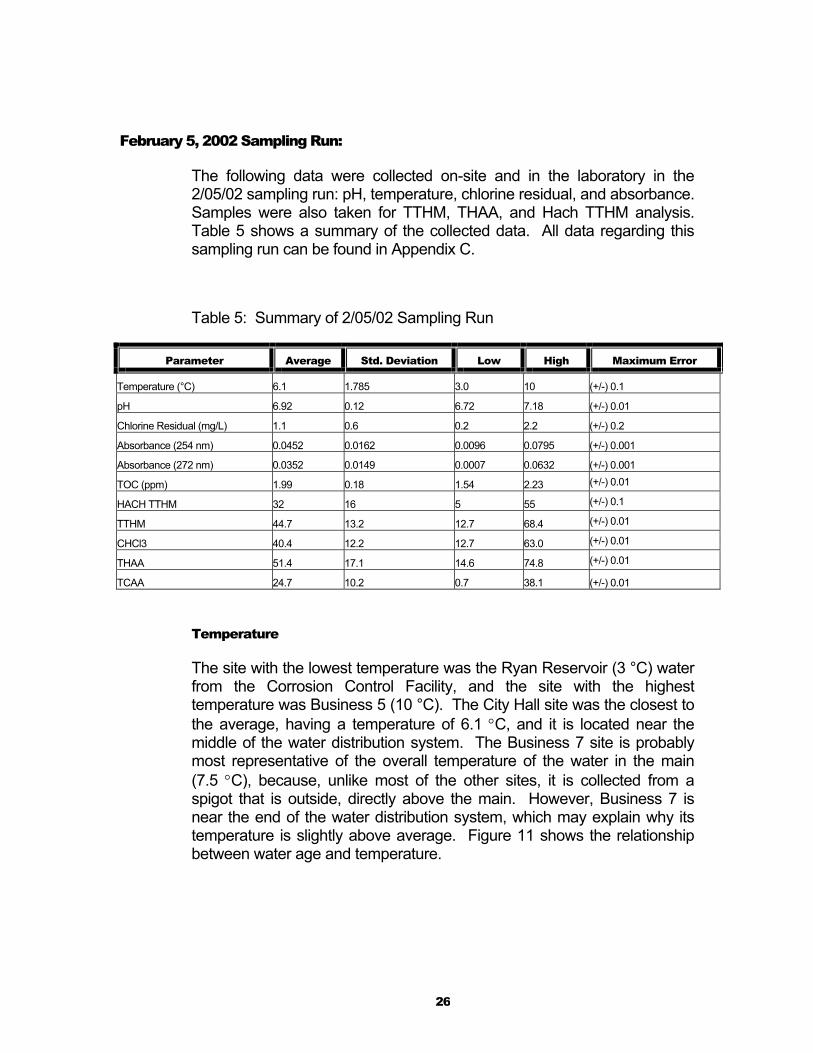
February 5, 2002 Sampling Run:

The following data were collected on-site and in the laboratory in the 2/05/02 sampling run: pH, temperature, chlorine residual, and absorbance. Samples were also taken for TTHM, THAA, and Hach TTHM analysis. Table 5 shows a summary of the collected data. All data regarding this sampling run can be found in Appendix C.

Table 5: Summary of 2/05/02 Sampling Run

Parameter Average Std. Deviation Low High Maximum Error

Temperature (°C) 6.1 1.785 3.0 10 (+/-) 0.1

pH 6.92 0.12 6.72 7.18 (+/-) 0.01

Chlorine Residual (mg/L) 1.1 0.6 0.2 2.2 (+/-) 0.2

Absorbance (254 nm) 0.0452 0.0162 0.0096 0.0795 (+/-) 0.001

Absorbance (272 nm) 0.0352 0.0149 0.0007 0.0632 (+/-) 0.001

TOC (ppm) 1.99 0.18 1.54 2.23 (+/-) 0.01

HACH TTHM 32 16 5 55 (+/-) 0.1

TTHM 44.7 13.2 12.7 68.4 (+/-) 0.01

CHCl3 40.4 12.2 12.7 63.0 (+/-) 0.01

THAA 51.4 17.1 14.6 74.8 (+/-) 0.01

TCAA 24.7 10.2 0.7 38.1 (+/-) 0.01

Temperature

The site with the lowest temperature was the Ryan Reservoir (3 °C) water from the Corrosion Control Facility, and the site with the highest temperature was Business 5 (10 °C). The City Hall site was the closest to the average, having a temperature of 6.1 °C, and it is located near the middle of the water distribution system. The Business 7 site is probably most representative of the overall temperature of the water in the main (7.5 °C), because, unlike most of the other sites, it is collected from a spigot that is outside, directly above the main. However, Business 7 is near the end of the water distribution system, which may explain why its temperature is slightly above average. Figure 11 shows the relationship between water age and temperature.

26

Figure 11: Water Age vs. Temperature (02/05/02)

Water Age (hours)

0 20 40 60 80 100 120 140 160

Tem

pera

ture

(o C)

2

4

6

8

10

12

pH

The highest pH was measured to be 7.18 at the Florence Fire Station. Business 8 also had a relatively high pH (7.15). The lowest pH recorded was 6.72 and was measured at the Water Department, where the service main is ductile iron. Business 3 represents the average of the system, with a pH of 6.93. Figure 12 shows how pH varies throughout the system.

27

Figure 12: Water Age vs. pH (02/05/02)

Water Age (hours)

0 20 40 60 80 100 120 140 160

pH

6.6

6.7

6.8

6.9

7.0

7.1

7.2

7.3

Chlorine Residual

The highest chlorine residual was measured to be 2.2 mg/L of free chlorine and was found to be in the water leaving the Leeds Chlorinator and at Manufacturer 1. The lowest chlorine residual was measured at Business 8 and was found to be 0.2 mg/L. The sites that are closest to the average chlorine residual (1.1 mg/L) are the Florence Fire Station, City Hall, Business 4, and the Hampshire County Jail, each having a measured chlorine residual of 1.0 mg/L. Figure 13 shows the relationship between measured chlorine residual and water age.

28

Figure 13: Water Age vs. Measured Chlorine Residual (02/05/02)Water Age (hours)

0 20 40 60 80 100 120 140 160

Chl

orin

e R

esid

ual (

mg/

L)

0.0

0.5

1.0

1.5

2.0

2.5

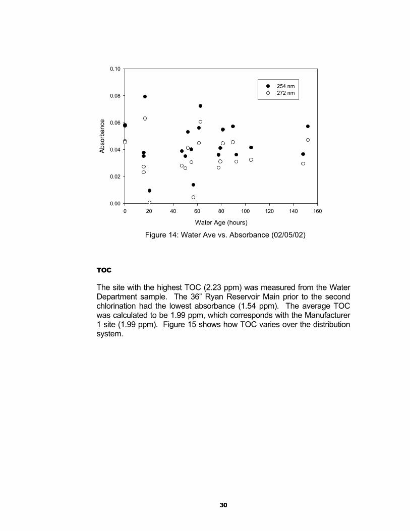
Differential UV spectroscopy

Samples for UV analysis were taken from every site, including the raw water sources, and were quenched with NH4Cl crystals. The site with the highest absorbance at both 254 nm and 272 nm was the Manufacturer 1 (0.0795 and 0.0632, respectively), and the site with the lowest absorbance at both 254 nm and 272 nm was the sample taken from Business 1 (0.0096, 0.0007 nm, respectively) after the last chlorination input. The average absorbance was calculated to be 0.0452 and 0.0352 at 254 nm and 272 nm, respectively. None of the samples are within (+/-) 0.004 of the calculated average absorbance. Figure 14 shows the relationship between water age and absorbance for 254 and 272 nm.

29

Water Age (hours)

0 20 40 60 80 100 120 140 160

Abso

rban

ce

0.00

0.02

0.04

0.06

0.08

0.10

254 nm272 nm

Figure 14: Water Ave vs. Absorbance (02/05/02)

TOC

The site with the highest TOC (2.23 ppm) was measured from the Water Department sample. The 36” Ryan Reservoir Main prior to the second chlorination had the lowest absorbance (1.54 ppm). The average TOC was calculated to be 1.99 ppm, which corresponds with the Manufacturer 1 site (1.99 ppm). Figure 15 shows how TOC varies over the distribution system.

30

Figure 15: Water Age vs. TOC (02/05/02)

Water Age (hours)

0 20 40 60 80 100 120 140 160

TOC

(ppm

)

1.7

1.8

1.9

2.0

2.1

2.2

2.3

Colorimetric TTHM Analysis

The results on this test were inconclusive because some of the data was lost. The data was analyzed on two separate dates (02/06/02 and 02/07/02) and the data from 02/07/02 was lost, leaving only 11 sites with measurements. The average concentration of TTHMs was 32.4 ppm, which had no corresponding value in the dataset. The minimum TTHM concentration was recorded at Business 6 (5 ppm), and the maximum concentration was recorded at the State Hospital (55 ppm). The relationship between the remaining data and the modeled water residence time is shown in Figure 16.

31

Figure 16: Water Age vs. Hach TTHM Concentration (02/05/02)

Water Age (hours)

0 20 40 60 80 100 120 140 160

TTH

M (p

pb)

0

10

20

30

40

50

60

TTHM and THAA

TTHM and THAA data were collected in duplicate and analyzed within two weeks of collection. Samples from the inflow to the Leeds Chlorinator and the initially chlorinated 36” Ryan Reservoir water main were lost, and thus are not included in this analysis. The site with the lowest TTHM and CHCl3 concentrations (12.7 ppb and 12.7 ppb, respectively) was the field- chlorinated 20” Mountain Street water main, and the site with the highest concentrations (68.4 ppb and 63.0 ppb, respectively) was the Florence Fire Station. The site with the lowest THAA and TCAA concentrations (14.6 ppb and 0.7 ppb, respectively) was the 20” Mountain Street water main, and the site with the largest (74.8 ppb and 37.7 ppb, respectively) was Manufacturer 1. Business 9 also had significantly high THAA and TCAA levels (72.5 ppb and 38.1 ppb, respectively). Figure 17 shows the relationship between DBP formation and water age in the distribution system.

32

Figure 17: Water Age vs. DBP Concentrations (02/05/02)

Water Age (hours)

0 20 40 60 80 100 120 140 160

DBP

(ppb

)

20

30

40

50

60

70

80

TTHMTHAA

TTHM and THAA Kinetics Data

Water samples were taken from the Corrosion Control Facility for a kinetics test. Pre-corrosion control water (that is, water that was chlorinated at the reservoirs yet had no additional treatment) was taken for the lab-chlorinated kinetics test. Post-corrosion control water (i.e., water that had undergone pH adjustment and additional chlorination at the CCF and goes to Northampton without further treatment) was also taken from the CCF. The post-CC water sample was brought to the lab and allowed to continue its reactions under well-controlled circumstances (samples were held headspace-free in a light-blocking incubator at 20 °C). Samples were taken at approximately 2, 6, 24, 48, 96, 120, 144, and 168 hours. Figures 18a and 18b show the results of the post-CC water chlorination kinetics tests. The pre-CC water samples were chlorinated at 3.0 mg/L and partitioned into three sets (these samples are referred to as “lab-chlorinated”). The first set had no pH adjustment done to it, the second was adjusted to a pH of 7, and the third was adjusted to a pH of 7.8 (the target pH was 8.5, but it was not reached). Sub-samples were then taken from each set of the lab-chlorinated water at 1, 2, 3, 5, and 7 days, and were analyzed for pH, chlorine residual, and THM and HAA concentration. Due to experimental difficulties, the 168 hour non pH adjusted sample was lost. Samples without pH adjustment tended to be extremely close to pH

33

7, so the data for the non-adjusted samples was averaged with pH=7 samples. Consequently, Figures 19a and 19b show only pH 7 and pH 8.5

Figure 18a: Site Chlorinated Kinetics TTHM Concentration (02/05/02)

Water Age (hours)

0 20 40 60 80 100 120 140 160 180 200

TTH

M (p

pb)

30

40

50

60

70

80

90

100

Ryan ReservoirMountain Street Reservoir

Figure 18b: Site Chlorinated Kinetics THAA Concentration (02/05/02)

Water Age (hours)

0 20 40 60 80 100 120 140 160 180

THAA

(ppb

)

30

40

50

60

70

80

90

34

Figure 19a: Lab Chlorinated and pH Adjusted Kinetics TTHM Concentrations (02/05/02)Water Age (hours)

0 20 40 60 80 100 120 140 160 180

TTH

M (p

pb)

25

30

35

40

45

50

55

60

65 Ryan Reservoir, pH 7Ryan Reservoir, pH 7.8Mountain Street Reservoir, pH 7Mountain Street Reservoir, pH 7.8

Figure 19b: Lab Chlorinated and pH Adjusted Kinetics THAA Concentrations (02/05/02)

Water Age (hours)

0 20 40 60 80 100 120 140 160 180

THAA

(ppb

)

10

20

30

40

50

60

Model

Several changes were made to the previously discussed version of the water distribution system model. First, accurate demands were assigned to each node that historically consumed large volumes of water (such as the local college and Manufacturer 2). The accurate demands were

35

determined by examining the water records for each site in town. The water volume remaining was divided over the remaining nodes, thus creating uniform demand for all other points in the distribution system. Other changes include the addition of the two wells into the model, as well as the addition of several service connections that are found in Northampton, although were not included in the model. Table 6 shows the water age, chlorine residual, and trace from the model with respect to each site.

Table 6: Summary of Model Output

Trace

Site Name Water Age (hrs) % Ryan % Mtn. St. % Well

1 % Well 2

Chlorine Residual (mg/L)

20" Mtn. St. RAW N/A 0 0 100.0 0.0 0

36" Ryan Res. RAW N/A 0 100 0.0 0.0 0

20" Mtn. St. CCF 0 100 0 0.0 0.0 1.8

36" Ryan Res. CCF 0 0 100 0.0 0.0 1.3

Leeds Chlorinator Inflow 15.5 0 100 0.0 4.1 1.2

Leeds Chlorinator Outflow 15.5 0 100 0.0 4.1 1.2

Manufacturing Plant 1 16.6 0 100 0.0 4.6 1.1

Business 1 20.4 0 100 0.0 4.1 1.1

Florence Fire Station 47.4 90.4 9.5 0.0 0.9 0.8

Business 2 50.2 78.9 21 0.0 7.7 0.7

Business 3 52.3 35.5 64.4 0.0 6.1 0.6

Water Dept. 55.1 82 17.8 0.0 6.2 0.6

Business 4 61.4 99.9 0 0.0 0.1 0.6

City Hall 62.8 99.6 0.3 3.2 0.1 0.6

Manufacturing Plant 2 79.3 49.8 50 0.0 5.7 0.4

State Hospital 77.7 99.9 0 15.8 0.1 0.3

State Police Barracks 81.4 36.8 63.1 0.0 6.1 0.3

Business 5 89.8 83 16.8 0.0 6.0 0.4

Hampshire County Jail 56.9 99.9 0 23.1 0.0 0.5

Business 6 104.8 49.7 50 1.8 2.4 0.4

Business 7 92.6 70.5 29.4 29.8 0.1 0.1

Business 8 148.1 99.7 0 15.8 0.0 0.3

Business 9 152 95.6 4.2 2.2 1.8 0.3

36

Table 7 shows a comparison between the modeled system and the actual water distribution system.

Table 7: Northampton Water Distribution System

Outflow (GPM) Initial Chlorine Dose (mg/L) Pressure (psi)

Site Name Measured Modeled Measured Modeled Measured Modeled

Ryan Reservoir 1000-1400 1605 1.3 1.3 - - Mountain Street Reservoir 1400-1710 417 1.8 1.8 - - Leeds Chlorination Station 1400-1740 417 1.8 0 - - Well 1 (Clark Street) 88 112 0 0 130 110.9 Well 2 (Spring Street) 108 92 0 0 100 61.4

Figure 20: Measured and Modeled Chlorine Residual vs. Modeled Water Age (02/05/02 )

Water Age (hours)

0 20 40 60 80 100 120 140 160

Chl

orin

e R

esid

ual (

mg/

L)

0.0

0.5

1.0

1.5

2.0

2.5

Water Age vs Measured Cl2 Res. Water Age vs Modeled Cl2 Res.

Y = 2.015 * e -0.125 *X

Y = 1.535 * e -0.0166 * X

Figure 20 shows how the measured chlorine residual compares to the modeled chlorine residual.

37

June 28, 2002 Well Sampling:

The two groundwater wells that serve Northampton were sampled along with the finished water from the Ryan Reservoir main and the Mountain Street main. Samples were analyzed for major cations and anions by ion chromatography. The results are in Table 8

Anion and Cation Analysis

Both wells are located in Florence, MA, and are approximately one mile apart. Well 1 is the Clark Street well, which, at the time of sampling, recorded a temperature of 13 °C. Well 2 is the Spring St. Extension well, which had a temperature of 12 ºC. Additionally, samples of the zinc orthophosphate and sodium hydroxide were taken from the corrosion control facility and brought back to the laboratory. Tests were then run on these two chemicals to determine the affect they have on treated water absorbance.

DBP Kinetics Test

A kinetics test was run on the well waters. Several aliquots of each well water were taken, with the first aliquot having no pH adjustment, the second adjusted to a pH of 7, and the third adjusted to a pH of 8.5. These samples were then split into two chlorination doses: 0.5 mg/L and 1.5 mg/L. Sub-samples were then taken from each sets of the lab-chlorinated water at 1, 2, 3, 5, and 7 days, and were analyzed for pH, chlorine residual, THM concentration, and HAA concentration. Figures 21a and 21b show the TTHM and THAA concentrations brought about by chlorinating and pH adjusting the sample of Well 1 water.

38

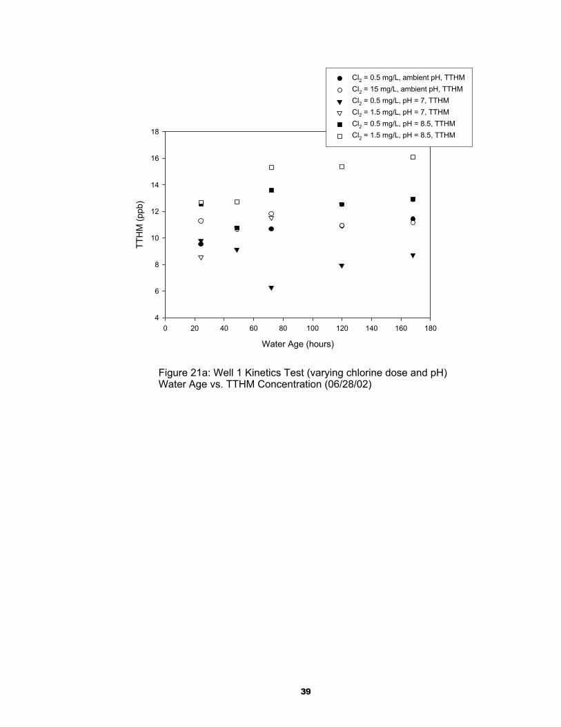
Figure 21a: Well 1 Kinetics Test (varying chlorine dose and pH) Water Age vs. TTHM Concentration (06/28/02)

Water Age (hours)

0 20 40 60 80 100 120 140 160 180

TTH

M (p

pb)

4

6

8

10

12

14

16

18

Cl2 = 0.5 mg/L, ambient pH, TTHM Cl2 = 15 mg/L, ambient pH, TTHM Cl2 = 0.5 mg/L, pH = 7, TTHM Cl2 = 1.5 mg/L, pH = 7, TTHM Cl2 = 0.5 mg/L, pH = 8.5, TTHM Cl2 = 1.5 mg/L, pH = 8.5, TTHM

39

Figure 21b: Well 1 Kinetics Test (varying chlorine dose and pH) Water Age vs. THAA Concentration (06/28/02)

Water Age (hours)

0 20 40 60 80 100 120 140 160 180

THAA

(ppb

)

4

6

8

10

12

14

16

18

Cl2 = 0.5 mg/L, ambient pH, THAACl2 = 1.5 mg/L, ambient pH, THAACl2 = 0.5 mg/L, pH = 7, THAACl2 = 1.5 mg/L, pH = 7, THAACl2 = 0.5 mg/L, pH = 8.5, THAACl2 = 1.5 mg/L, pH = 8.5, THAA

Table 8: Anion and Cation Analysis

Sample Ca (mg/L) Mg (mg/L) Na (mg/L) K (mg/L) Cl (mg/L) SO4 (mg/L)

Mountain Street Main 7.25 0.97 4.74 0.72 6.31 6.46

Ryan Reservoir Main 6.86 0.88 6.12 0.62 4.86 5.89 Well 1 15.61 3.5 6.87 1.25 22.14 12.41 Well 2 11.68 2.48 3.79 0.92 5.29 7.9

February 2, 2003 Anion Analysis

Raw water samples from both reservoirs were analyzed for sulfate and fluoride concentration using the ion chromatography (EVE instrument). Table 9 contains the anion analysis for the Ryan Reservoir and Mountain Street raw waters. All data regarding this test are in Appendix E.

40

Table 9: Sulfate and Fluoride Concentration in Both Reservoirs

Site Sulfate (ppm) Fluoride (ppb)

Mountain St. Reservoir 0.9 42.8 Ryan Reservoir 1.0 59.0

March 4, 2003 Sampling Run:

The following data was collected on-site and in the laboratory in the 3/4/03 sampling run: pH, temperature, chlorine residual, absorbance, TTHM concentration, THAA concentration. Additionally, the absorbance of samples passed through different solid phase extraction tubes was recorded. Table 10 shows a summary of the collected data. Appendix F has all data from this sampling date.

Table 10: Summary of 3/04/03 Sampling Run

Parameter Average Std. Deviation Maximum Minimum Max Error

Temperature (ºC) 4.6 1.235 9.000 3.000 (+/-) 0.1

pH 6.830 0.248 7.770 6.440 (+/-) 0.01 Cl2 Residual (mg/L) 0.954 0.558 1.900 0.000 (+/-) 0.2 TTHM (ppb) 40.8 17.7 0.0 88.0

THAA (ppb) 43.4 19.1 0.0 67.9

254 Abs. 0.039 0.011 0.068 0.000

272 Abs. 0.031 0.010 0.057 0.000

Filt. 254 Abs. 0.040 0.007 0.063 0.034

Filt. 272 Abs. 0.032 0.006 0.054 0.026

Sax 254 0.002 0.002 0.000 0.007 Sax 272 0.002 0.002 0.000 0.006 Sax 254 Filt 0.011 0.013 0.001 0.045 Sax 272 Filt 0.010 0.012 0.000 0.040 Diol 254 0.030 0.007 0.024 0.048 Diol 272 0.022 0.007 0.016 0.041 Diol 254 Filt 0.029 0.005 0.022 0.042 Diol 272 Filt 0.021 0.005 0.015 0.034

41

Temperature

The temperature was taken for this sampling run on March 4th, which was a relatively warm day. With the exception of the Hampshire County Jail and the State Hospital samples, all samples had temperatures of under 6 ºC. The average temperature of the water samples was calculated to be 4.6 ºC, which corresponds with the Mountain Street chlorination station. The highest water temperature recorded was 9 ºC at the State Hospital, and the lowest water temperature was 3 ºC, which was recorded at the Ryan Reservoir chlorination station. Figure 22 shows the temperature variation over the distribution system.

Figure 22: Water Age vs. Temperature (03/04/03)

Water Age (hours)

0 20 40 60 80 100 120 140 160

Tem

pera

ture

(o C)

3

4

5

6

7

8

9

10

pH

The pH of all of the samples was measured in the laboratory the day of sampling. Manufacturer 1 and Business 1 represent the average of the system with a pH pf 6.83. The Business 8 site had the highest pH: 7.77. The Ryan Reservoir chlorination station had the lowest pH, a measurement of 6.44. Other sites with high pH values are Business 9, Florence Fire Station, and the State Hospital. The latter two are usually problematic because they have very wide or long service connections, and

42

it is suspected that the system does not flush easily. Figure 23 shows the pH variability across the distribution system.

Figure 23: Water Age vs. pH (03/04/03)

Water Age (hours)

0 20 40 60 80 100 120 140 160

pH

6.4

6.6

6.8

7.0

7.2

7.4

7.6

7.8

8.0

Chlorine Residual

Previously, a HACH colorimetric kit was used to determine the chlorine residuals in the distribution system. However, in months prior to the sampling run, new HACH kits (the Pocket Colorimeter II) were purchased and placed into use. The average chlorine residual was measured to be 0.954 mg/L, which corresponds to the Florence Fire Station. The maximum chlorine residual was measured to be 1.90 mg/L at the Leeds Chlorinator Outflow, Manufacturer 1, and in both of the mains at the Corrosion Control Facility. The minimum chlorine residuals were 0 mg/L and 0.07 mg/L, taken at both reservoir chlorination facilities and at Business 8, respectively. Figure 24 shows the chlorine residual across the distribution system. The two outliers seen in Figure 24 are the State Hospital and the State Police Barracks.

43

Figure 24: Water Age vs. Measured Chlorine Residual (03/05/03)

Water Age (hours)

0 20 40 60 80 100 120 140 160

Chl

orin

e R

esid

ual (

mg/

L()

0.0

0.5

1.0

1.5

2.0

TTHM and THAA

Samples were collected in triplicate, stored at 4ºC, and analyzed in duplicate within two weeks. One of the City Hall and Manufacturer 1 samples were lost due to bottle leakage during the extraction process, calling the results for the remaining two into doubt. The highest TTHM and THAA values occurred at Business 8 (88.0 and 67.9 ppb, respectively). The lowest TTHM and THAA concentrations were at the both reservoirs chlorination stations, and were 0 ppm for both. The next lowest TTHM concentration (26.7 ppb) was measured at the inflow to the Leeds Chlorination Facility, and the next lowest THAA concentration (31.9 ppb) was measured at the outflow to the Leeds Chlorination Facility. Figure 25 shows the DBPs across the distribution system.

44

Water Age (hours)

0 20 40 60 80 100 120 140 160

DBP

s (p

pb)

0

20

40

60

80

100

TTHMTHAA

Figure 25: Water Age vs. DBP Concentration (03/05/03)

Absorbance

Samples were quenched with 0.1 M sodium sulfite and analyzed over the course of several days. The absorbance for the unfiltered 36” main raw water was 0.068 at 254 nm and 0.057 at 272 nm. The absorbance for the unfiltered 20” main water was 0.049 at 254 nm and 0.042 at 272 nm. The unfiltered sampling site waters ranged from 0.051 to 0 at 254 nm, and 0.043 to 0 at 272 nm. The absorbance for the filtered 36” main raw water was 0.063 at 254 nm and 0.054 at 272 nm. The absorbance for the filtered 20” main water was 0.046 at 254 nm and 0.039 at 272 nm. The filtered sampling site waters ranged from 0.41 to 0.034 at 254 nm, and 0.044 to 0.026 at 272 nm. Of all of the sampling sites, the State Hospital had the largest filtered and unfiltered absorbance. Figure 26 shows the absorbance as it varies across the distribution system for at 254 and 272 nm.

45

Figure 26: Water Age vs. Absorbance (03/04/03)

Water Age (hours)

0 20 40 60 80 100 120 140 160

Abs

orba

nce

0.020

0.025

0.030

0.035

0.040

0.045

0.050

0.055

UV Absorbance at 254 nmUV Absorbance at 272 nm

Fractionation of Organic Matter

Two commercially-available adsorbents were investigated: an anion exchange resin (LC-SAX) and a hydrophilic resin (LC-DIOL). While these adsorbents required different procedures (as explained in the Methods section), the approach was the same. Samples were adjusted as needed to the appropriate pH for each sample. Each tube was conditioned using 20 mL of Super-Q water adjusted to sample pH, and the sample waters were then run through the tubes. The effluent was retained and the absorbance measured. The data for these tests are in Table 10.

Statistical Modeling

Once data had been gathered, SigmaStat, a statistical analysis program, was used to explore correlations between TTHM and THAA concentrations and the results from the Solid Phase Extraction Tube. Over three hundred correlations were run, using chlorine residual, temperature, pH, filtered and non-filtered absorbance (for both the site samples and the effluent from the solid phase extraction tubes) as the

46

independent variables. All of the correlations can be found in the appendix; the best one TTHMs is listed in Table 11. The form of the model presented in Table 11 is shown below:

DBP = 10A*[Cl2 Residual(mg/L)]B*[Temperature (°C)]C*[LC-Diol Effluent at 254 nm]D (5)

Table 11: NOM Fractionation Results

Parameter Values

Independent Variable

A B C D r2

DIOL TTHM 0.947 0.311 -0.238 -0.53 0.812

No successful correlations between the THAA and various independent variables were found. It was attempted to correct the HAA data to take biodegradation into account, but this method also did not work. Additionally, there were no successful correlations when the LC-Sax resin was included in the analysis. Several sites were not included in the analysis due to either lack of data or uncertainty in the data. These sites were the unchlorinated water mains, Business 2, Manufacturer 1, City Hall, Business 7 and Business 5.

DATA ANALYSIS & DISCUSSION

October 16, 2001 Sampling Run

Temperature

It is expected that the temperature of the water in the distribution system will change from the initial intake to the sampling sites because the ground acts as an insulator from the air temperature. Although the tap water was run for as much as 10 minutes at some sites before sampling, the large temperature variance (seen both in Figure 1 and Table 1) suggests that either we were not entirely successful in measuring water from the main or

47

that the water temperature in the distribution system increases with time (possibly due to ground temperature).

pH

pH variability can affect production of disinfection by-products, although no link was found in this analysis. The measured pH variability (seen in Figure 2 and in Table 1) in the water distribution system is most likely due to the size of the service pipe entering the building, the residence time of the water in the pipe, and the composition of the pipe. The composition of the water main in the Florence Fire Station area is cast iron, although the service connection composition is mostly asbestos cement. The diameter of the service connection is unusually large at 6 inches. While the water in the service connection is periodically flushed by the Fire Department, the average residence time of the water in the service connection is abnormally large at this location. During this time, the water could react with the asbestos cement walls, potentially raising the pH of the water. While the purpose of running the tap for 10 minutes at this site was to flush the service connection and get a representative sample of water from the main, the high pH indicates that this might not have been completely successful. Business 8 does not have a large service connection, and is one of the last sites before the end of Northampton’s water main, in an area where the water demand is low. It is suspected that water going to sites at the edges of the distribution system moves slower through the water mains, possibly raising the pH (although the water main in question is made of cast iron).

Chlorine Residual

It is expected that the smallest chlorine residuals occur when the water retention time is greatest, because chlorine decays and reacts with organic material in the water over time. Therefore, the older a water is the smaller the residual will be because it will be reacting with organic materials and decaying via other processes. In this case, the time was taken from the model output; no tracer study has been conducted to determine absolute water retention times for Northampton. This is especially apparent in Figure 3, which shows how the residual varies with water retention time.

48

TOC

Generally, the total organic carbon in a water distribution system will decrease with time. There are two main reasons for this decrease: reaction with chlorine and biodegradation. First, when chlorine reacts with organic material, it creates TTHMs and HAAs, and oxidizes a small amount of the natural organic material to CO2. Second, some dissolved organic carbon is biodegradable, and at advanced water ages (where the chlorine residual is small), attached biomass may accumulate in the distribution system and consume the DOC as a food source. This would then drive the TOC down.

Instantaneous DBPs

Figure 6 shows that as the water age increases, there is a slight increase in TTHMs and HAAs for the first 48 hours. However, beyond that point there is no clear trend in the TTHMs and possibly a slight decreasing trend in the HAAs.

DBP Formation Kinetics

Water age for the site chlorinated samples is the time from arrival at the CCF. By this point the water has experienced several hours of chlorine contact as it traveled from the chlorination stations in Williamsburg to the Northampton CCF For this reason, the earliest samples all showed substantial DBP formation (Figures 8a and 8b). The laboratory chlorinated samples were also exposed to chlorination in the field, and contact in the transmission mains. However, these were supplemented with additional chlorine (3 mg/L and 6 mg/L dose) under well-controlled laboratory conditions. All show a clear progression of increasing DBP concentration with increasing contact time. They also show an increase in DBP formation with increasing chlorine dose, as well as higher levels from Ryan Reservoir as compared to Mountain Street. These differences were more pronounced for the THMs than for the HAAs.

Biodegradation can account for some of the inconsistencies in the data. Sites affected by biodegradation are expected to show a decrease in THAA concentration, but not TTHM concentration. Examining the ratio between THAA and TTHM concentrations may indicate the sites where biodegradation is occurring, because the ratio between the two will decrease as biodegradation comes into play. In Figure 27, the ratio remains relatively constant except at low residuals (where the chlorine

49

concentration is not high enough to suppress biological activity). The State Hospital and Business 7 are two sites where the ratio is low, and thus biodegradation is believed to occur. Another way to examine the effect of biodegradation on a water distribution system is to compare THAA concentration and the chlorine residual of the system, as seen in Figure 28. It is expected that a system with little or no biological activity the distribution system would show that as the chorine residual decreases the THAA concentration increases and eventually levels off where the chlorine residual is zero. Northampton’s water distribution system follows this with the exception of three sites, which, given their reduced THAA concentration, suggests that biodegradation is occurring. These three sites are Business 8, Business 7, and the State Hospital. Other sites that vary from the relationship between the THAA concentration and the chlorine residual are the State Police Barracks and Business 9.

Figure 27: Chlorine Residual vs. THAA/TTHM ratio (10/16/01)

Chlorine Residual (mg/L)

0.0 0.5 1.0 1.5 2.0 2.5

THA

A/T

THM

0.0

0.5

1.0

1.5

2.0

50

Chlorine Residual (mg/L)

0.0 0.5 1.0 1.5 2.0 2.5

THAA

Con

cent

ratio

n (p

pb)

10

20

30

40

50

60

70

80

Figure 28: Chlorine Residual vs. THAA (10/16/01)

Distribution System Modeling

The model was primarily used by trying to match the observed chlorine residuals with the modeled chlorine residuals. However, there are several problems with this approach. First, the two groundwater wells in Northampton’s water distribution system are not yet included in the model. This has the effect of possibly lowering the chlorine residual in the actual distribution system, but not affecting it in the model (which can be observed in Figure 7). Second, only the water mains are included in the hydraulic model of the water distribution system. Discrepancies between modeled and measured residuals could also be due to long service connections between the water main and the tap (as is the case with the site at the Hampshire County Jail and the State Hospital). Third, the modeled demand data is simply the average daily use divided over all of the nodes. This too could cause the modeled chlorine residual (as well as the water age) results to be incorrect, by assuming that a neighborhood consisting of many nodes uses more water than the entire industrial section in Northampton. Fourth, the rate constant for chlorine used in the model is not the rate constant that is most appropriate for the system. Finally, biodegradation is not included in the model, even though it is

51

suspected to be present in the distribution system. With systems in place to compensate for these inconsistencies between the actual and modeled distribution system, the model will be more accurate at predicting correct residence times and chlorine residuals.

February 5, 2002 Sampling Run:

General

The relationship between temperature and water age are approximately the same as the October 16, 2001 sampling run: in general, temperature increases with distance (and time) away from the Corrosion Control Facility. The chlorine residual decayed at a similar rate as the previous sampling run. There was no clear relationship between the modeled water age and TOC concentration. This could be due to biodegradation.

TTHM and THAA

Figure 17 shows the TTHM and THAA concentration over time. It was expected to see that as the water retention time increased the THAA and TTHM concentration would also increase. When examining Figure 17, it is apparent that while this trend does occur, other factors are probably influencing the formation of TTHM and THAAs (such as pH, temperature, biodegradation, etc.). The highest THAA concentration occurred at Manufacturer 1 and the highest TTHM concentration was at Florence Fire Station. The lowest (non-raw and immediately chlorinated waters) concentrations for TTHM and THAA occurred at Business 6 and the Leeds Chlorinator, respectively.

Kinetics

It was expected that the concentration of DBPs would increase over time, which is true for the TTHMs and generally true for the THAAs. Figures 19a and 19b show the lab chlorinated and pH adjusted TTHM and THAA kinetics data. In these figures it is clear that the TTHMs have a clear relationship between TTHM formation and water residence time. The THAAs also have a similar relationship, although there is more variability.

52

Colorimetric TTHM Method

A comparison between the colorimetric TTHM analysis and the TTHM samples analyzed by GC is in Figure 29. In the colorimetric TTHM method, the manual lists several compounds that interfere with the measurements for TTHM concentration. For compounds that interfere positively (thus inflating the estimated TTHM concentration) are dibromochloroacetic acid, dichlorobromoacetic acid, tribromoacetic acid, and trichloroacetic acid, all of which are HAA compounds. Since the HAAs at the Northampton site are usually in high concentrations, it would be expected that the measured colorimetric TTHM concentrations will be higher than the TTHMs measured using the standard method. Unfortunately, this is not the case, as the colorimetric TTHM concentrations were all lower than the TTHMs using the standard method.

Figure 29: TTHM (analyzed by Hach Method) vs. TTHM (analyzed by GC) (02/05/02) Hach TTHM (ppb)

0 10 20 30 40 50 60

TTH

M (p

pb)

30

35

40

45

50

55

60

65

Model

As age and tracer data are not available for the water distribution system, a comparison between the modeled and measured chlorine residual is probably the best way to assess the accuracy of the model. However, even this assessment has its limitations, because our modeling of the measured chlorine residual does not take several key factors into account. First, while the two groundwater wells in Northampton’s water distribution system have been included in the model their pressure and discharge are not correct. The modeled wells are pumping water at a low rate over a 24 hour period rather than pumping at a high rate for 6 hours, which is how

53

the wells are actually used in the distribution system. This may explain the discrepancy between the observed and modeled well pressures and has the possible effect of showing a different modeled chlorine residual than a measured one. Second, while some of the service connections are included in the hydraulic model of the water distribution system, not all are. For example, a map of the service connections at the Hampshire County Jail showed that there was a connection between Rocky Hill Rd. and Burt’s Pit Road. Adding this connection helped make the modeled and measured chlorine residual data more similar, although it is not known whether or not the addition of this connection completed the model. Fourth, the rate constant for chlorine used in the model is not site-specific, and therefore will exhibit some systematic error. Finally, biodegradation is not included in the model, even though it is suspected to occur in the distribution system.

DBP formation has been found to be directly proportional to the drop in UV absorbance of a chlorinated water (Li, Chi-Wang, et al. 1998). This value, called the differential UV absorbance (delta-UV), reflects the amount of change in absorbance brought about by the chlorination reaction with organic material. The delta-UV was calculated using the results from the trace analysis performed by the model as shown:

∆UV272 = (MA) - [(%RR)*UVRR+(%MR)*UVMtnR]/100 (6)

Where MA is the measured absorbance at 272 nm at a specific site in the distribution system, %RR and %MR are the percentages of the water at the site that come from the Ryan Reservoir and the Mountain Street Reservoir, respectively. UVRR and UVMtnR are the measured raw water absorbance values at 272 nm for the Ryan Reservoir and the Mountain Street Reservoir, respectively. Data displaying the calculated delta-UV is in the appendix and in Figure 30. Figure 30 shows that as the ∆UV272 becomes more positive the TTHM concentration increases while the THAA concentration increases only slightly. This suggests that there is a relationship between TTHM concentration and ∆UV272 absorbance value but not between THAA concentration and ∆UV272 absorbance value.

54

Delta UV at 272 nm

-0.04 -0.03 -0.02 -0.01 0.00 0.01 0.02 0.03 0.04

DBP

s (p

pb)

30

40

50

60

70

80

THAATTHM

Figure 30: Delta-UV 272 vs. DBP concentration (02/05/02)

June 28, 2002 Well Sampling:

The primary purpose of sampling the wells and finding the anion and cation concentration in the well and reservoir waters was to determine whether or not a natural source exists for a tracer study. While there were some differences in the concentrations of anions and cations, ultimately the differences were not large enough to make them useful as tracers. The only possible exception to this was the sulfate, which was extremely large for the Mountain Street finished water main. However, the technicians at the lab noticed this difference, and tested the Mountain Street samples of sulfate over time. The technicians noticed that when the Mountain Street sample was exposed to air, the sulfate concentration increased, suggesting that the concentration measured (after exposure to air) was not the concentration in the pipes. The reasons for this are not clear.

February 2, 2003 Anion Analysis

Given the consistency between the sources for both fluoride and sulfate, there was no good candidate for a natural tracer test.

55

March 4, 2003 Sampling Run

The statistical modeling performed for the March 4th run was much more successful than previous runs. One reason for this may be that the Northampton Water Department switched to a chlorine residual measuring system that uses an instrumental colorimeter (instead of a method based on visual perception of color) to make the chlorine residual measurement. Since the concentration of chlorine in the water is related to the disinfection byproduct concentration, a stronger relationship between the two can be evaluated. This relationship came into play when the statistical modeling of the standard absorbance and the absorbance from the SPE resins was examined. Appendix F has the multiple linear regression data sheets for the best correlations. The P value on this sheet refers to how significant each coefficient is. The lower the P value the more important the value. In all of the statistical analyses for this sampling run the chlorine residual was by far the most significant variable. Adding the LC-Diol effluent did not improve the results.

56

CONCLUSIONS

1) The use of hydraulic distribution system models coupled with laboratory chlorination tests is a powerful technique for assessing DBP formation in medium-sized drinking water utilities.

2) The colorimetric THM method shows promise, although chemical interferences appeared to be a problem at times.

3) Solid phase extraction coupled with absorbance measurements holds promise for characterizing the degree of NOM oxidation, and therefore the amount of DBP formation. More study is needed here.

4) Differential UV absorbance was not successful as a surrogate for DBP formation, nor did it help when combined with other methods.

57

Appendices

Appendix B: Collected Data for Northampton 10/16/01Site Name Date Water Age % Ryan % Mtn. St. Temp (oC) Cl2 Residual Modeled Cl2 pH TOC (ppm)20" Mtn. St. RAW 10/16/01 0 100 6.96 2.23336" Ryan Res. RAW 10/16/01 100 0 6.64 2.10420" Mtn. St. Chlorinated 10/16/01 0 100 0 2.07 2.90 7.29 2.42336" Ryan Res. Chlorinated 10/16/01 0 0 100 1.02 3.10 6.87 2.265Leeds Chlorinator 10/16/01 15.52 0 100 18.9 2.20 2.20 7.03 2.408Manufacturing Plant 1 10/16/01 15.98 0 100 16.1 1.70 2.10 7.08 2.239Business 1 10/16/01 22.06 0 100 15.5 1.10 1.80 7.1 2.208Florence Fire Station 10/16/01 45.45 90.4 9.5 15 0.30 1.50 8.71 2.2Business 2 10/16/01 49.08 78.9 21 15.5 0.70 1.20 7.06 2.247Business 3 10/16/01 51.37 35.5 64.4 15.5 0.80 0.90 7.06 2.154Water Dept. 10/16/01 53.56 82 17.8 16.7 1.00 1.10 6.96 2.037Business 4 10/16/01 60.66 99.9 0 17.5 0.70 0.90 6.99 2.152City Hall 10/16/01 62.03 99.6 0.3 16.7 0.60 0.70 6.94 2.183Manufacturing Plant 2 10/16/01 75.71 49.8 50 18.3 0.50 0.50 7.12 2.105State Hospital 10/16/01 78.68 99.9 0 21 0.10 0.60 6.86 1.098State Police Barraks 10/16/01 82.2 36.8 63.1 18 0.30 0.30 7.19 2.066Business 5 10/16/01 90.37 83 16.8 19 0.50 0.50 7.15 2.05Hampshire County Jail 10/16/01 98.34 99.9 0 17 1.10 0.60 6.89 2.212Business 6 10/16/01 105.34 49.7 50 19 0.40 0.30 6.94 2.173Business 7 10/16/01 107.01 70.5 29.4 18 0.10 0.30 6.55 1.541Business 8 10/16/01 146.57 99.7 0 17 0.10 0.50 8.5 1.689Business 9 10/16/01 150.85 95.6 4.2 20 0.20 0.50 7.05 2.035

Appendix B: Collected Data for Northampton 10/1Site Name CHCl3 CHCl2Br CHClBr2 TTHM20" Mtn. St. RAW 25.65 3.99 0.24 29.8936" Ryan Res. RAW 45.18 5.40 0.35 50.9420" Mtn. St. Chlorinated 103.76 9.94 0.49 114.1936" Ryan Res. Chlorinated 39.12 5.66 0.33 45.11Leeds Chlorinator 58.13 7.62 0.43 66.17Manufacturing Plant 1 30.80 4.76 0.33 35.89Business 1 50.25 7.25 0.45 57.95Florence Fire Station 65.01 8.11 0.48 73.60Business 2 70.97 7.88 0.46 79.30Business 3 58.21 7.33 0.47 66.01Water Dept. 65.68 7.06 0.42 73.17Business 4 39.07 5.65 1.20 45.93City Hall 63.02 6.92 0.42 70.35Manufacturing Plant 2 4.22 0.61 0.00 4.83State Hospital 58.43 7.05 0.48 65.96State Police Barraks 63.37 7.62 0.48 71.46Business 5 56.04 6.59 0.41 63.03Hampshire County Jail 79.96 8.37 0.52 88.86Business 6 0.00 0.00 0.00 0.00Business 7 55.38 6.66 0.43 62.46Business 8 43.13 6.66 1.09 50.89Business 9 66.09 9.11 0.98 76.18

Appendix B: Kinetics Data for Northampton 10/16/01Chlorinated at chlorination station, then stopped decay in lab over timeTime (hrs) CHCl3 CHCl2Br CHClBr2 CHBr3 TTHM

1.5 46.4 5.4 0.3 0.0 52.26 53.3 5.9 0.3 0.0 59.5

24 55.5 6.0 0.3 0.0 61.848 56.1 5.8 0.3 0.0 62.2

Ryan Reservoir 76 63.7 3.0 1.0 1.2 68.896 63.3 6.4 0.3 0.0 70.0120 61.3 6.0 0.3 0.0 67.6144 63.1 6.0 0.3 0.0 69.4192 64.8 6.1 0.3 0.0 71.31.5 36.4 5.0 0.3 0.0 41.76 43.9 5.6 0.4 0.0 49.9

24 46.8 5.8 0.3 0.0 52.9Mountain Street Reservoir 48 51.0 6.1 0.4 0.0 57.4

76 54.0 6.1 0.3 0.0 60.496 58.3 6.8 0.4 0.0 65.5120 57.1 6.4 0.4 0.0 63.9144 56.7 6.2 0.4 0.0 63.2192 59.5 6.2 0.4 0.0 66.1

59

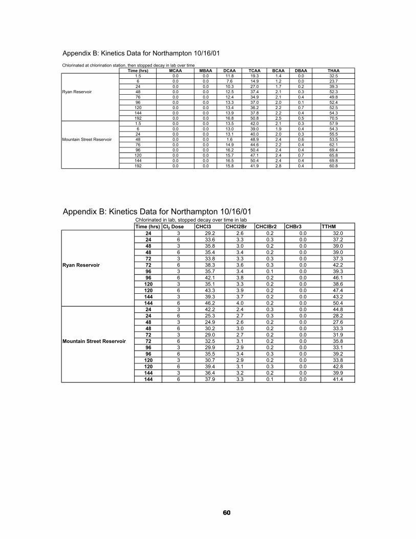
Appendix B: Kinetics Data for Northampton 10/16/01Chlorinated at chlorination station, then stopped decay in lab over time

Time (hrs) MCAA MBAA DCAA TCAA BCAA DBAA THAA1.5 0.0 0.0 11.8 19.3 1.4 0.0 32.56 0.0 0.0 7.6 14.9 1.2 0.0 23.7

24 0.0 0.0 10.3 27.0 1.7 0.2 39.3Ryan Reservoir 48 0.0 0.0 12.5 37.4 2.1 0.3 52.3

76 0.0 0.0 12.4 34.9 2.1 0.4 49.896 0.0 0.0 13.3 37.0 2.0 0.1 52.4

120 0.0 0.0 13.4 36.2 2.2 0.7 52.5144 0.0 0.0 13.9 37.8 2.2 0.4 54.3192 0.0 0.0 16.8 50.8 2.5 0.5 70.51.5 0.0 0.0 13.5 42.0 2.1 0.3 57.96 0.0 0.0 13.0 39.0 1.9 0.4 54.3

24 0.0 0.0 13.1 40.0 2.0 0.3 55.5Mountain Street Reservoir 48 0.0 0.0 1.6 48.9 2.4 0.6 53.5

76 0.0 0.0 14.9 44.6 2.2 0.4 62.196 0.0 0.0 16.2 50.4 2.4 0.4 69.4

120 0.0 0.0 15.7 47.1 2.4 0.7 65.8144 0.0 0.0 16.5 50.4 2.4 0.4 69.8192 0.0 0.0 15.8 41.9 2.8 0.4 60.8

Appendix B: Kinetics Data for Northampton 10/16/01Chlorinated in lab, stopped decay over time in labTime (hrs) Cl2 Dose CHCl3 CHCl2Br CHClBr2 CHBr3 TTHM

24 3 29.2 2.6 0.2 0.0 32.024 6 33.6 3.3 0.3 0.0 37.248 3 35.8 3.0 0.2 0.0 39.048 6 35.4 3.4 0.2 0.0 39.072 3 33.8 3.3 0.3 0.0 37.3

Ryan Reservoir 72 6 38.3 3.6 0.3 0.0 42.296 3 35.7 3.4 0.1 0.0 39.396 6 42.1 3.8 0.2 0.0 46.1

120 3 35.1 3.3 0.2 0.0 38.6120 6 43.3 3.9 0.2 0.0 47.4144 3 39.3 3.7 0.2 0.0 43.2144 6 46.2 4.0 0.2 0.0 50.424 3 42.2 2.4 0.3 0.0 44.824 6 25.3 2.7 0.3 0.0 28.248 3 24.9 2.6 0.2 0.0 27.648 6 30.2 3.0 0.2 0.0 33.372 3 29.0 2.7 0.2 0.0 31.9

Mountain Street Reservoir 72 6 32.5 3.1 0.2 0.0 35.896 3 29.9 2.9 0.2 0.0 33.196 6 35.5 3.4 0.3 0.0 39.2

120 3 30.7 2.9 0.2 0.0 33.8120 6 39.4 3.1 0.3 0.0 42.8144 3 36.4 3.2 0.2 0.0 39.9144 6 37.9 3.3 0.1 0.0 41.4

60

Appendix B: Kinetics Data for Northampton 10/16/01Chlorinated in lab, stopped decay over time in labTime (hrs) Cl2 Dose MCAA MBAA DCAA TCAA BCAA DBAA THAA

24 3 1.3 0.0 5.4 27.2 1.4 0.1 35.324 6 0.0 0.0 7.6 29.5 1.7 0.2 39.048 3 0.0 0.0 6.9 31.9 1.0 0.2 39.948 6 0.0 0.0 9.8 33.3 0.4 0.1 43.672 3 0.0 0.0 8.1 37.3 2.0 0.2 47.5

Ryan Reservoir 72 6 0.0 0.0 10.7 39.4 1.8 0.4 52.396 3 0.0 0.0 10.6 42.2 0.8 0.1 53.796 6 0.0 0.0 11.2 46.7 0.9 0.1 59.0120 3 0.0 0.0 9.2 41.1 2.7 0.3 53.3120 6 0.0 0.0 9.6 44.2 1.3 0.2 55.3144 3 0.0 7.9 39.6 0.3 0.1 47.9144 6 0.0 0.0 7.5 43.4 1.1 0.4 52.324 3 7.2 0.0 6.3 32.2 1.1 0.4 47.224 6 2.6 0.0 8.4 35.6 1.4 0.3 48.348 3 0.0 0.0 7.6 33.5 1.7 0.2 43.048 6 0.0 0.0 11.0 37.6 1.4 0.2 50.272 3 0.0 0.0 9.7 35.9 2.8 0.4 49.0

Mountain Street Reservoir 72 6 0.0 0.0 12.1 43.4 1.6 0.2 57.396 3 0.0 0.0 11.9 39.5 2.8 0.4 54.796 6 0.0 0.0 13.9 48.1 1.7 0.2 64.0120 3 0.0 0.0 10.9 37.9 2.2 0.2 51.1120 6 0.0 0.0 10.4 47.2 0.1 0.0 57.7144 3 0.0 1.3 36.6 0.5 0.3 38.7144 6 0.0 8.4 42.3 0.8 0.2 51.8

Appendix C: Collected Data for Northampton 02/05/02Site Name Date Water Age % Ryan % Mtn % Well 1 % Well 2 Modeled Cl2 Temp (oC) Cl2 Residual TOC (ppm)20" Mtn. St. RAW 02/05/02 0.0 100.0 0.0 0.0 0 4.0 0.0 1.59436" Ryan Res. RAW 02/05/02 100.0 0.0 0.0 0.0 0 3.5 0.0 1.54120" Mtn. St. Chlorinated 02/05/02 0 0.0 100.0 0.0 0.0 1.8 4.0 1.8 2.18536" Ryan Res. Chlorinated 02/05/02 0 100.0 0.0 0.0 0.0 1.3 3.0 1.3 1.918Leeds Chlorinator Inflow 02/05/02 15.54 0.6 95.3 0.0 4.1 1.2 4.2 2.2 2.025Leeds Chlorinator Outflow 02/05/02 15.54 0.6 95.3 0.0 4.1 1.2 4.1 1.8 2.041Manufacturing Plant 1 02/05/02 16.56 0.1 95.3 0.0 4.6 1.1 4.6 2.2 1.988Business 1 02/05/02 20.42 0.6 95.3 0.0 4.1 1.1 5.1 1.6 2.123Florence Fire Station 02/05/02 47.35 99.1 0.0 0.0 0.9 0.8 5.2 1.0 1.748Business 2 02/05/02 50.2 81.1 11.2 0.0 7.7 0.7 6.0 1.2 2.205Business 3 02/05/02 52.3 33.4 60.5 0.0 6.1 0.6 5.1 1.3 1.838Water Dept. 02/05/02 55.07 84.8 9.0 0.0 6.2 0.6 4.7 1.2 2.232Business 4 02/05/02 61.42 99.9 0.0 0.0 0.1 0.6 8.0 1.0 2.045City Hall 02/05/02 62.75 96.6 0.1 3.2 0.1 0.6 6.1 1.0 2.085Manufacturing Plant 2 02/05/02 79.27 65.2 29.1 0.0 5.7 0.4 5.4 0.8 2.024State Hospital 02/05/02 77.72 84.1 0.0 15.8 0.1 0.3 8.0 0.4 2.006State Police Barraks 02/05/02 81.36 35.6 58.3 0.0 6.1 0.3 6.5 0.3 2.155Business 5 02/05/02 89.75 85.1 8.9 0.0 6.0 0.4 10.0 0.6 1.971Hampshire County Jail 02/05/02 56.86 76.9 0.0 23.1 0.0 0.5 7.0 1.0 2.15Business 6 02/05/02 104.84 92.2 3.6 1.8 2.4 0.4 8.0 0.5 1.873Business 7 02/05/02 92.56 70.1 0.0 29.8 0.1 0.1 7.5 0.3 1.801Business 8 02/05/02 148.07 84.2 0.0 15.8 0.0 0.3 7.5 0.2 2.009Business 9 02/05/02 151.98 93.5 2.5 2.2 1.8 0.3 8.0 0.5 2.132

61

Appendix C: Collected Data for Northampton 02/05/02Site Name pH Abs. 254 nm Abs. 272 nm MCAA MBAA DCAA TCAA BCAA DBAA THAA20" Mtn. St. RAW 6.98 0.0373 0.0319 11.5 0.7 0.8 0.7 0.8 0.2 14.636" Ryan Res. RAW 6.95 0.0515 0.0464 12.020" Mtn. St. Chlorinated 7.09 0.0582 0.0465 9.5 1.6 12.9 12.9 1.3 0.2 38.336" Ryan Res. Chlorinated 6.93 0.0578 0.0456 11.9 1.3 12.1 10.8 2.0 0.1 38.2Leeds Chlorinator Inflow 6.84 0.0353 0.0231 7.3 1.2 13.2 13.0 1.4 0.2 36.3Leeds Chlorinator Outflow 7.00 0.0377 0.0274Manufacturing Plant 1 6.98 0.0795 0.0632 9.5 0.9 24.9 37.6 1.6 0.2 74.8Business 1 6.94 0.0096 0.0007 8.0 0.6 17.9 21.9 1.8 0.2 50.4Florence Fire Station 7.18 0.0389 0.0282 12.0 0.3 13.0 12.0 1.3 0.2 38.8Business 2 6.84 0.0352 0.0262 8.1 0.8 22.4 31.9 1.6 0.2 64.9Business 3 6.93 0.0531 0.0413 13.8 0.5 19.7 27.7 1.4 0.1 63.4Water Dept. 6.72 0.0403 0.0307 5.1 0.9 23.4 31.7 2.9 1.3 65.3Business 4 6.87 0.0561 0.0448 8.3 0.8 22.7 32.2 1.7 0.2 65.8City Hall 6.95 0.0724 0.0606 5.1 0.8 21.1 29.2 1.6 0.1 57.9Manufacturing Plant 2 6.77 0.0412 0.0312 6.2 0.9 20.6 30.0 1.4 0.2 59.4State Hospital 6.87 0.0362 0.0265 5.6 0.8 15.8 23.0 1.2 0.1 46.6State Police Barraks 7.08 0.0549 0.0447 4.5 1.1 24.3 36.5 1.6 0.2 68.2Business 5 6.86 0.0573 0.0455 5.0 0.8 23.9 33.8 1.8 0.1 65.6Hampshire County Jail 6.85 0.0139 0.0047 9.2 0.6 18.1 22.5 1.6 0.1 52.2Business 6 6.81 0.0417 0.0325 4.4 0.9 19.4 26.5 1.5 0.2 52.8Business 7 6.73 0.0362 0.0310 3.0 0.7 15.5 18.2 1.2 0.2 38.7Business 8 7.15 0.0367 0.0297 4.2 1.0 19.2 27.6 1.4 0.2 53.7Business 9 6.88 0.0573 0.0473 6.2 1.2 25.1 38.1 1.7 0.2 72.5

Appendix C: Collected Data for Northampton 02/05/02Site Name CHCl3 CHCl2Br CHClBr2 CHBr3 TTHM HACH TTHM20" Mtn. St. RAW 12.7 0.0 0.0 0.0 12.736" Ryan Res. RAW20" Mtn. St. Chlorinated 29.3 2.5 0.3 0.0 32.136" Ryan Res. Chlorinated 20.0 3.1 0.2 0.0 23.3Leeds Chlorinator Inflow 31.3 3.2 0.7 0.0 35.2Leeds Chlorinator OutflowManufacturing Plant 1 38.8 4.1 0.1 0.0 43.0Business 1 42.9 4.3 0.7 0.0 47.9 43Florence Fire Station 63.0 5.0 0.5 0.0 68.4Business 2 40.2 4.1 0.4 0.0 44.8 20Business 3 50.8 4.5 0.6 0.0 56.0Water Dept. 33.4 4.4 0.6 0.0 38.4 18Business 4 47.8 4.2 0.2 0.0 52.2City Hall 33.3 4.0 0.4 0.0 37.7 22Manufacturing Plant 2 53.8 4.6 0.3 0.0 58.7State Hospital 42.7 3.8 0.3 0.0 46.8 55State Police Barraks 44.8 4.7 0.4 0.0 49.9 39Business 5 45.2 3.9 0.3 0.0 49.5Hampshire County Jail 45.6 4.1 0.3 0.0 49.9 41Business 6 30.2 3.9 0.4 0.0 34.5 5Business 7 33.0 3.7 0.6 0.0 37.3 18Business 8 52.9 4.9 0.5 0.0 58.2 43Business 9 56.4 5.1 0.5 0.0 62.0 52

62

Appendix C: Kinetics Test 02/05/02Site Chlorinated Kinetics Test (2/5/02) Results

Time (hrs) Cl2 Res. CHCl3 CHCl2Br CHClBr2 CHBr3 TTHM MCAA MBAA DCAA TCAA BCAA DBAA THAAMnt. 0 1.79 23.3 11.8 0.5 0.0 35.6 8.8 1.6 3.1 46.7 2.0 0.2 62.4Mnt. 7 1.42 37.1 17.1 0.4 0.0 54.6 7.4 0.4 15.4 16.0 1.3 0.2 40.8Mnt. 24 1.21 35.4 18.3 0.5 0.0 54.2 7.9 0.5 16.9 19.0 1.7 0.3 46.4Mnt. 48 1.05 36.1 18.1 0.5 0.0 54.7 7.7 0.8 17.9 18.4 1.6 0.3 46.7Mnt. 72 0.75 42.0 21.5 0.7 0.0 64.2 9.9 1.0 21.6 24.5 1.8 0.2 58.9Mnt. 96 0.7 44.4 22.1 0.6 0.0 67.2 8.5 1.1 20.7 23.3 1.6 0.1 55.3Mnt. 120 0.67 45.4 22.7 0.6 0.0 68.6 9.3 1.2 21.7 25.4 1.6 0.1 59.2Mnt. 168 50.2 24.1 0.6 0.0 74.9 8.6 1.3 22.6 25.4 1.6 0.1 59.7Mnt. 173 0.84 52.3 24.7 0.6 0.0 77.6Ryan 2 1.28 47.3 20.1 0.6 0.0 68.0 11.7 0.4 20.4 27.9 1.6 0.2 62.3Ryan 6 49.7 13.4 0.5 0.0 63.6 9.9 0.5 20.1 27.5 2.1 0.1 60.2Ryan 24 1.2 43.8 21.2 0.5 0.0 65.4 7.3 0.7 24.1 31.3 2.2 0.2 65.8Ryan 48 0.99 49.0 24.5 0.7 0.0 74.2 9.4 0.9 25.7 37.5 2.2 0.2 75.9Ryan 96 0.86 50.8 28.7 0.7 0.0 80.1 7.8 0.8 29.4 42.9 2.5 0.2 83.7Ryan 120 0.8 54.3 26.3 0.7 0.0 81.3 6.6 1.1 23.9 34.7 1.6 0.1 67.9Ryan 144 0.76 57.8 27.3 0.8 0.0 85.9 8.5 1.3 27.1 41.3 1.7 0.1 80.1Ryan 168 60.1 28.3 0.8 0.0 89.2 7.9 1.4 29.3 42.1 1.9 0.2 82.8

63

2/5/2002 TTHM Lab Chlorinated Kinetics Results (Chlorinated at 3 mg/L)M.S

Sample Time CHCl3 CHCl2Br CHClBr2 CHBr3 TTHM Cl2 Res. pHno pH 24 26.7 4.09 0.44 0 31.2 1.92 7.14pH=7 24 23.4 3.44 0.38 0 27.2 1.95 7.02

pH=8.5 24 27.0 3.70 0.45 0 31.2 2.01 7.71no pH 48 27.3 4.01 0.46 0 31.7 2.18 7.05pH=7 48 25.0 3.64 0.36 0 29.0 1.42 7.04

pH=8.5 48 28.4 3.86 0.39 0 32.7 2.16 7.88no pH 72 28.7 4.19 0.48 0 33.4 1.69 6.99pH=7 72 26.8 3.95 0.35 0 31.1 1.68 7.01

pH=8.5 72 33.2 4.45 0.43 0 38.1 1.55 7.82no pH 120 31.8 4.55 0.43 0 36.7 1.53 6.98pH=7 120 31.1 4.54 0.45 0 36.1 1.55 7.01

pH=8.5 120 36.2 4.64 0.47 0 41.3 1.5 7.77no pH 168 35.9 4.96 0.38 0 41.3 0.92 6.92pH=7 168 34.2 4.82 0.40 0 39.4 1.4 6.96

pH=8.5 168 39.3 4.71 0.45 0 44.4 1 7.69

Concentrations

R.RSample Time CHCl3 CHCl2Br CHClBr2 CHBr3 TTHM Cl2 Res. pHno pH 24 31.5 4.60 0.45 0 36.6 1.8 7.1pH=7 24 32.6 5.13 0.52 0 38.3 1.84 7.02

pH=8.5 24 35.3 4.95 0.48 0 40.7 1.98 7.79no pH 48 36.1 5.52 0.59 0 42.2 1.78 7.07pH=7 48 32.9 4.97 0.38 0 38.3 1.68 7.01

pH=8.5 48 39.8 5.24 0.40 0 45.5 1.6 7.8no pH 72 38.3 5.71 0.52 0 44.6 1.61 6.98pH=7 72 35.3 5.21 0.42 0 40.9 1.67 7.02

pH=8.5 72 41.7 5.48 0.46 0 47.6 1.65 7.87no pH 120 39.5 5.70 0.49 0 45.7 1.56 6.94pH=7 120 46.5 6.83 0.55 0 53.9 1.62 7.02

pH=8.5 120 49.3 6.31 0.56 0 56.1 1.5 7.82

pH=7 168 46.1 6.45 0.42 0 53.0 1.26 7.07

Concentrations

Appendix D: Collected Data for Northampton 06/28/02Site Name Date Temp (°C) Cl2 Residual pHWell 1 6/28/2002 13 0 6.25Well 2 6/28/2002 12 0 6.3320" Mountain St. Chlorinated 6/28/2002 19 1.21 7.5536" Ryan Res. Chlorinated 6/28/2002 17 0.82 7.45

64

Appendix D: Kinetics Results for Well 1 06/28/02TTHMs

Time (hours) Cl2 = 0.5, ambient pH Cl2 = 1.5, ambient pH Cl2 = 0.5, pH = 7 Cl2 = 1.5, pH = 7 Cl2 = 0.5, pH = 8.5 Cl2 = 0.5, pH = 8.524 9.5 11.3 9.8 8.6 12.6 12.748 10.7 10.7 9.1 10.8 10.8 12.772 10.7 11.8 6.3 11.5 13.6 15.3120 10.9 11.0 7.9 12.5 12.5 15.4168 11.4 11.1 8.7 12.9 12.9 16.1

THAAsTime (hours) Cl2 = 0.5, ambient pH Cl2 = 1.5, ambient pH Cl2 = 0.5, pH = 7 Cl2 = 1.5, pH = 7 Cl2 = 0.5, pH = 8.5 Cl2 = 0.5, pH = 8.5

24 14.1 14.7 11.1 14.7 5.7 12.648 6.7 13.5 11.2 13.6 13.6 9.472 11.3 13.1 11.4 12.6 8.0 11.2120 10.4 15.1 11.9 14.7 14.7 9.4168 8.5 11.2 12.5 15.8 15.8 8.4

Appendix E: Sulfide and Flouride Analysis of Ryan and Mountain Street Reservoirs 2/3/03

STANDARDS RESERVOIR WATERSulfide Sulfide Area ppm

ppm Area Mtn: 1.81E+08 0.900 0 Ryan: 1.99E+08 1.00

0.1 26211831 Flouride Area ppb1 2.41E+08 Mtn: 1811317 42.8

10 3.61E+09 Ryan: 2497206 59.0

Flourideppb Area

0 080 3255943

100 4340811

Sulfide (IC Standards Calibration)

y = 4E+08xR2 = 1

0.000.501.001.502.002.503.003.504.00

0 2 4 6 8 10 12

Concentration (ppm)

Are

a (b

illio

ns)

StandardsRyanMountainLinear (Standards)

Flouride (IC Standards Calibration)

y = 42351xR2 = 0.9972

0

1

2

3

4

5

0 20 40 60 80 100 120

Concentration (ppb)

Are

a (m

illio

ns)

StandardsRyanMountainLinear (Standards)

65

Appendix F: Collected Data for Northampton 03/04/03Site Name Date Cl2 Res. Temp (oC) pH TTHM (ppm) THAA (ppm) UV Abs. 254 nm UV Abs. 272 nm20" Mtn. St. RAW 03/04/03 0 4.6 6.71 0 0 0.049 0.04236" Ryan Res. RAW 03/04/03 0 3 6.44 0 0 0.068 0.05720" Mtn. St. Chlorinated 03/04/03 1.77 3.6 6.76 29 47 0.036 0.02736" Ryan Res. Chlorinated 03/04/03 1.58 3.6 6.97 37 48 0.038 0.03Leeds Chlorinator Inflow 03/04/03 1.35 4.2 6.72 27 34 0.037 0.028Leeds Chlorinator Outflow 03/04/03 1.9 4.3 6.58 28 32 0.037 0.029Manufacturing Plant 1 03/04/03 1.78 4.5 6.83 32 16 0.04 0.031Business 1 03/04/03 1.54 4.3 6.83 40 46 0.036 0.026Florence Fire Station 03/04/03 0.96 3.6 6.95 47 56 0.041 0.033Business 2 03/04/03 1.1 4.8 6.93 45 58 0.042 0.032Business 3 03/04/03 1.07 3.4 6.8 44 55 0.039 0.031Water Dept. 03/04/03 1.14 5 6.88 42 34 0.044 0.035Business 4 03/04/03 1.03 4.3 6.77 45 53 0.038 0.029City Hall 03/04/03 1.03 4.7 6.72 45 15 0.04 0.031Manufacturing Plant 2 03/04/03 0.89 4.1 6.89 41 48 0.042 0.034State Hospital 03/04/03 0.23 9 6.95 55 55 0.051 0.043State Police Barraks 03/04/03 0.46 3.7 6.67 55 59 0.04 0.031Business 5 03/04/03 0.87 5.9 3.78 48 58 0.039 0.03Hampshire County Jail 03/04/03 1.1 6 6.74 41 53 0.036 0.027Business 6 03/04/03 0.79 5.5 6.66 50 58 0 0Business 7 03/04/03 0.72 4 6.74 47 54 0.037 0.029Business 8 03/04/03 0.07 5.4 7.77 88 68 0.038 0.028Business 9 03/04/03 0.57 4.8 6.95 49 54 0.039 0.03

Appendix F: Collected Data for Northampton 03/04/03Site Name Filt. UV Abs. 254 nm Filt. UV Abs. 272 nm UV Abs. Sax 254 UV Abs. Sax 272 Filt. UV Abs. Sax 25420" Mtn. St. RAW 0.046 0.039 0.002 0.001 0.00636" Ryan Res. RAW 0.063 0.054 0 0 0.00120" Mtn. St. Chlorinated 0.035 0.027 0 0 0.04536" Ryan Res. Chlorinated 0.037 0.029 0.005 0.005 0.006Leeds Chlorinator Inflow 0.038 0.029 0.002 0.002 0.038Leeds Chlorinator Outflow 0.034 0.026 0.005 0.004 0.028Manufacturing Plant 1 0.041 0.032 0.007 0.006 0.004Business 1 0.034 0.027 0.001 0.001 0.003Florence Fire Station 0.047 0.038 0.002 0.001 0.006Business 2 0.039 0.032 0.001 0 0.008Business 3 0.039 0.03 0.003 0.002 0.007Water Dept. 0.04 0.032 0.001 0.001 0.003Business 4 0.037 0.029 0.004 0.003 0.006City Hall 0.037 0.028 0.003 0.002 0.013Manufacturing Plant 2 0.04 0.032 0.001 0 0.005State Hospital 0.049 0.041 0.0019176 0.00085075 0.00842285State Police Barraks 0.037 0.029 0.002 0.001 0.004Business 5 0.035 0.027 0.00280075 0.00208585 0.0282364Hampshire County Jail 0.043 0.036 0.0022125 0.0016403 0.004Business 6 0.004 0.003 0.003Business 7 0.037 0.029 0.00351335 0.0026764 0.028885Business 8 0.037 0.029 0.00183865 0.00138855 0.002Business 9 0.036 0.029 0.0020523 0.0016174 0.0065

66

Appendix F: Collected Data for Northampton 03/04/03Site Name Filt. UV Abs. Sax 27 UV Abs. Diol 254 UV Abs. Diol 272 Filt. UV Abs. Diol 254 Filt. UV Abs. Diol 27220" Mtn. St. RAW 0.005 0.034 0.026 0.035 0.02736" Ryan Res. RAW 0 0.044 0.035 0.043 0.03420" Mtn. St. Chlorinated 0.04 0.024 0.017 0.022 0.01536" Ryan Res. Chlorinated 0.005 0.028 0.019 0.029 0.02Leeds Chlorinator Inflow 0.034 0.028 0.021 0.034 0.027Leeds Chlorinator Outflow 0.026 0.026 0.018 0.025 0.018Manufacturing Plant 1 0.003Business 1 0.002 0.03 0.025 0.026 0.019Florence Fire Station 0.006 0.025 0.017 0.024 0.017Business 2 0.007 0.026 0.017 0.025 0.017Business 3 0.006 0.03 0.021 0.028 0.02Water Dept. 0.002 0.027 0.019 0.03 0.022Business 4 0.005 0.031 0.021 0.032 0.024City Hall 0.012 0.024 0.016 0.022 0.015Manufacturing Plant 2 0.004 0.028 0.02 0.028 0.021State Hospital 0.007927345 0.032 0.022 0.03 0.021State Police Barraks 0.003 0.03 0.021 0.03 0.022Business 5 0.02150725 0.048 0.041Hampshire County Jail 0.0045 0.031 0.022 0.031 0.022Business 6 0.003 0.026 0.018 0.025 0.017Business 7 0.032631 0.047 0.039Business 8 0.003 0.029 0.022 0.042 0.034Business 9 0.006 0.028 0.019 0.028 0.02

67