multi-attribute decision making analysis rensselaer
TRANSCRIPT
Multi-Attribute Decision Making Analysiswith Evolutionary ProgrammingApplied to Large Scale Vehicle II
by
Allan D. Andrew
B.S. Mechanical EngineeringNorthwestern University, 1988M.S. Mechanical Engineering
Rensselaer Polytechnic Institute, 1995
SUBMITTED TO THE DEPARTMENT OF OCEAN ENGINEERING IN PARTIALFULFILLMENT OF THE REQUIREMENTS FOR THE DEGREES OF
NAVAL ENGINEERAND
MASTER OF SCIENCE IN OCEAN SYSTEMS MANAGEMENTAT THE
MASSACHUSETTS INSTITUTE OF TECHNOLOGY
JUNE 1998
C Allan D. Andrew. All rights reserved.
The author hereby grants to MIT permission to reproduceand to distribute publicly paper and electronic
copies of this thesis document in whole or in part.
Signature of Author:_Department of Ocean Engineering
May 8, 1998
Certified by: i Alan J. BrownSenior Lecturer Naval Architecture and Marine Engineering
Thesis Supervisor
Certified by:_Harry A. Jackson
Senior LecturerThesis Reader
Accepted by:J. Kim Vandiver
Chairman, Committee on Graduate Students
MASSACHUSETTS INSTITUTE Department of Ocean EngineeringOF TECHNOLOGY
OCT 2 3 1998
LIBRARIES

Multi-Attribute Decision Making Analysis
with Evolutionary Programming
Applied to Large Scale Vehicle II
by
Allan D. Andrew
Submitted to the Department of Ocean Engineeringon May 8, 1998 in partial fulfillment of the
requirements for the degrees of Naval Engineer andMaster of Science in Ocean Systems Management
Abstract
Ship and submarine design is a very complicated process that requires many trade-offs indesign parameters in order to obtain the optimal vehicle effectiveness at the best cost.The number of potential designs is infinite, and the ship designer needs a tool to assist insearching this design space. This thesis uses an evolutionary program to determine theoptimal designs of Large Scale Vehicle II, a one-quarter scale submarine model used forpropulsor development. A set of designs is randomly generated and represented bybinary strings. Each design is treated as an individual in a biological population andevaluated for total ownership cost and two measures of effectiveness. Measures ofeffectiveness obtained through expert opinion and computer modeling are explored. Thedesigns with high effectiveness and low cost are chosen to produce offspring while thedesigns with poor effectiveness and high cost are removed from the population. Overmany generations, the designs that yield high effectiveness dominate the population. Nosingle design is identified as the optimum. Instead, the information is presented to thedecision-maker on a two-dimensional plot that represents the frontier of all non-dominated designs. Each axis represents one of the measures of effectiveness and eachlevel of cost is plotted on a separate curve. This process allows the decision-maker tochoose one or several of the non-dominated designs to continue through feasibility anddetailed design.
Thesis Supervisor: Alan J. BrownTitle: Senior Lecturer Naval Architecture and Marine Engineering
Acknowledgments
I would like to attempt to thank the many people who have been instrumental in thewriting of this thesis. Without the help of these many resources, my work at MIT wouldnot have been possible.
To Captain Alan Brown, his guidance as my thesis advisor provided valuable insight andlively discussion at our weekly meetings. Thank you for your guidance and good luck atVirginia Tech.
Thank you to Captain Harry Jackson for serving as my thesis reader. Much of the LSVcomputer model I used relies heavily upon the knowledge I gained from his course onSubmarine Design Trends. It was indeed an honor to be able to learn from a pioneer inthe field of submarine design.
Thanks must also be given to LCDR Greg Thomas of NAVSEA 03U for taking time outof his busy schedule to teach me about LSV II. His initiative in suggesting this projectwas extremely insightful. Also thanks for letting me tag along to experience a week inNAVSEA.
My sincere gratitude goes to LCDR Mark Thomas, who took the time to help meunderstand genetic algorithms and their potential application to the design of submarines.This thesis relies heavily upon the work he has done in pursuit of his Ph.D. at MIT.
Dr. Jeff Cohen and Mr. Walt Sadowski of Naval Underwater Warfare Center (NUWC)must be acknowledged for their valuable insight into the design decision process for NewAttack Submarine.
Most of all I wish to thank my loving wife. The support she has given me over our entirelife together, especially over the past three years, means more to me than anyone canknow. She is a wonderful wife and mother. I know our one-year-old son, Harrison, canhave no better care. What she does with him makes anything that I may accomplish palein comparison. To Stephanie, all my love, forever and always.

Table of Contents
ABSTACT ........... - ....... .............. 3
ACKNOWLEDGMENTS... ............- - ----..... ............- . . 4
TABLE OF CONTENTS ......................................... ......................
LIST OF FIGUES..............0 0.... ........ 7
LIST OF TABLES ..................... ... .
LIST OF SYMBOLS AND ABBREVIATIONS..................-- ........ ..... 9
1 INTRODUCTION . . - .... ........ ............... 11
1.1 B ACKGROUND ..................................................................................... ......... 11
1.2 EVOLUTIONARY PROGRAMS ..................................................................................................... 131.3 LARGE SCALE VEHICLE II ............................................... ................................................... 13
2 PREVIOUS AND CURRENT METHODS FOR CONCE'T SHIP DESIGN............ ...... 17
2.1 N SSN ..................................................................................................................................... 172.1.1 COEA Phase I .............................................................. 17
2.1.2 COEA Phase II................................................................................................................ 19
2.2 CVX ................................................. 20
2.3 LSV II ................................................... 232.4 COMPARISON WITH PROPOSED METHOD ............................................................................ 24
3 ................. ........... . .. .. .. .............. *..............25
3.1 OVERVIEW ................................................... 25
3.2 DESIGN PARAMETERS ................................................... 263.3 EFFECTIVENESS AND COST ............................................................................ 27
3.3.1 Cost...................................... 28
3.3.2 M easures of Effectiveness................................................................................................ 30
3.3.3 Combined Measure ofEffectiveness (CMOE) .................................. .............. 31
3.4 EVOLUTIONARY PROGRAM..................................................................... ................ 383.4.1 Evolutionary Program Background............................................................................. 38
3.4.2 Binary Representation ..................................................................................................... 41
3.4.3 First Generation.............................................................................................................. 42
3.4.4 Subsequent Generations............................................................ 43
3.5 PRESENTATION TO THE DECISION-MAKER ........................................ 46
4 DETAILED PROCESS ............................................ 49
4.1 DESIGN PARAMETERS .......................................................................... 49
4.2 BINARY REPRESENTATION ........................................... ...................................................... 51
4.3 RANDOM SELECTION OF FIRST GENERATION................................................................... 51
4.4 BALANCE AND FEASIBILITY OF DESIGN .......................................................................... 524.4.1 H ull Geometry.......... ...................................................................................... .... 52
4.4.2 Weights and InternalArrangements........................................................................... 54
4.4.3 Feasibility ................................. .................................... ................................................ 56
4.5 M EASURES OF PERFORMANCE ........................................... ................................................. 57
4.5.1 Vehicle Resistance........................................................................................................... 57
4.5.2 M axim um Speed ............................................................. ........................................... 594.5.3 Battery Energy Consumption ....................................... ........................................... 59
4.5.4 Hydroacoustic Runs ........ ................ ............... .................. 604 5 5 Hydrodynamic Runs .. .. . ... ............. ...... 62
4.6 C O ST .................................................................................................... . 634.6. 1 Acquisition Cost.................... ........... ................. ....... ..... ........................... 634.6.2 Discounted Total Ownership Cost.................. .......................... .................... 64
4.7 HYDROACOUSTIC M EASURE OF EFFECTIVENESS ............................................. ................... 654.8 HYDRODYNAMIC AND FLEXIBILITY COMBINED MEASURE OF EFFECTIVENESS .......................... 704.9 GENERATION OF NEW DESIGNS ........ ................................. 73
4.9.1 Selection of Parents and Lethals .............................. ... 744 9.2 Crossover and M utation .. ........................ . ............................ ..... 754.9. 3 Population .... ................... ....... ...... ..... .......... ................ . ........ 764.9.4 Non-D om inated Designs .............. .. .................. .................................................... ..... 77
4.10 DISPLAY OF INFORMATION ........................................................... 78
5 TUNING THE GENETIC ALGORITHM ................................................................................. 79
5.1 E X HA USTIV E SEA RCH ..................... ..................................................................... 795.1.1 Exhaustive Search Method......................................... ..... ................................. 80
5.2 TUNING THE G ENETIC A LGORITHM ............................................................................................... 805.2.1 G eneration S e. .................................. ........... ........................... ......... .815.2.2 Mutation Rate. ..................... ..................... ............ 835.2 3 Penalties for Injeasible Designs .. . .. .. . .. 845.2 4 Restart... . ................................................ 85
5.3 CONCLUSION .......... .... ............................................................................. ......... 86
6 R ESULTS ............................................................................................................................... . 87
6.1 OBJECTIVE ATTRIBUTE TRENDS ON THE PARETO FRONTIER ...................... .................. 876. 1 Pareto Frontier Plot Explanation......... .................. ...... ........... . .... 876.1.2 Pareto Frontier: Exhaustive Search ......... ......... .......... ...... ...................... 886.1.3 Margin as a Measure of Effectiveness .... ...............................................91
6.2 COMPARISON OF EVOLUTIONARY PROGRAM SEARCH TO EXHAUSTIVE SEARCH .......................... 946.3 EXPANDING THE DESIGN PARAMETER SPACE .......................................................... 101
6.3.1 Expanded Search ........... ...... .............................. ............................... 1026.4 FOCUSED SEARCH ......... ..... .................................................................................................... 105
6.4 1 Final Decision . ................... ........ ....... ..... ............................ 107
7 CONCLUSION ........................................................................................................ 113
BIBLIO G RA PH Y ........................... ........................................................................................... 117
APPENDIX A: EXPERT OPINION SURVEYS .................................................................................. 119
APPENDIX B: EXHAUSTIVE SEARCH DATA ................ ................... 129
APPENDIX C: FORTRAN CODE ........................................ 145
6
List of Figures
FIGURE 3-1 PARETO FRONTIER AND FEASIBLE DESIGN REGION FOR 2 OBJECTIVE ATTRIBUTES.................. 28
FIGURE 3-2 EXAMPLE ISO-EFFECTIVENESS CURVES............................................................................... 34
FIGURE 3-3 FLOW CHART FOR EVOLUTIONARY PROGRAM........................ ................... 39
FIGURE 3-4 PARETO FRONTIER wITH 3 OBJECTIVE ATTRIBUTES ....................................... .......... 47
FIGURE 4-1 HULL GEOMETRY ................................................................................................................ 52
FIGURE 4-2 INTERNAL ARRANGEMENTS DRAWING........................................................ 54
FIGURE 4-3BATTERY POWER RATINGS AS A FUNCTION OF TIME AT POWER................................ 60
FIGURE 4-4 EXPECTED dB UNCERTAINTY WITH MAX HYDROACOUSTIC SPEED 25 KNOTS ...................... 66
FIGURE 4-5 EXPECTED dB UNCERTAINTY WITH MAX HYDROACOUSTIC SPEED 30 KNOTS................... 67
FIGURE 4-6 ISO-EFFECTIVENESS WITH FROUDE RUNS CONSTANT........................................................... 73
FIGURE 4-7 ISO-EFFECTIVENESS WITH GEO-SIM CONSTANT.................................... .................. 73
FIGURE 4-8 MUTATION RATE AS AFUNCTION OF GENERATION.............................................................. 76
FIGURE 4-9 POPULATION OBJECTIVE ATTRIBUTE PENALTY AS A FUNCTION OF GENERATION ................. 77
FIGURE 5-1 EXHAUSTIVE SEARCH CHROMOSOMES...................................................... 80
FIGURE 5-2 AVERAGE TIME PER EVALUATION AS AFUNCTION OF GENERATION SIZE ............................ 81
FIGURE 5-3 PROGRAM PERFORMANCE WITH VARYING GENERATION SIZE COMPARED TO RANDOM SEARCH
...................................................................................................................................................... 83
FIGURE 5-4 PROGRAM PERFORMANCE WITH VARYING GENERATION SIZE ............................................. 83
FIGURE 5-5 PROGRAM PERFORMANCE WITH VARYING MUTATION RATE............................................... 84
FIGURE 5-6 PROGRAM PERFORMANCE WITH VARYING POPULATION PENALTIES ...................................... 85
FIGURE 5-7 PROGRAM PERFORMANCE COMPARING RESTART VS. LARGE NUMBER OF GENERATIONS ......... 86
FIGURE 6-1 PARETOFRONTIER: EXHAUSTIVE SEARCH ........................................ 89
FIGURE 6-2 PARTIAL PARETO FRONTIER: EXHAUSTIVE SEARCH W/ MARGIN AS MOE............................ 93
FIGURE 6-3 PARETO FRONTIER ESTIMATE (8,000 EVALS) ...................................................................... 95
FIGURE 6-4 PARETO FRONTIERESTIMATE (16,000 EVALS) ........................................ .......... 96
FIGURE 6-5 PARETO FRONTIER ESTIMATE (24,000 EVALS) .................................................................... 97
FIGURE 6-6 PARETO FRONTIER ESTIMATE (32,000 EVALS) ............................................................ 98
FIGURE 6-7 EVOLUTIONARY PROGRAM PERFORMANCE .................... ..................................................... 100
FIGURE 6-8 PARETO FRONTIER ESTIMATE: EXPANDED SEARCH............................................................ 104
FIGURE 6-9 PARETO FRONTIER ESTIMATE: FOCUSED SEARCH ..................................... 106
FIGURE 6-10 PARTIAL FRONTIER ESTIMATE: FOCUSED SEARCH............................................................ 108
FIGURE 6-11 ALL FEASIBLE DESIGNS AT $135M ..................................................................................110
List of Tables
TABLE 4-1 BATTERY CHARACTERISTICS ................................................................................................. 50TABLE 4-2 CHROMOSOME AND GENE SIZES FOR INITIAL MODEL.................... ...................... 51TABLE 4-3 HULL CHARACTERISTICS FOR NSSN AND SSN-21.................................. ................ 54TABLE 4-4 BATTERY SPECIFIC POWERS ............................................................................................ 55TABLE 4-5 COST ESTIMATING RELATIONSHIPS (CERs) ....................................... 64TABLE 4-6 RELATIVE BATTERY COST............................................................................................... 64TABLE 4-7 LIFE CYCLE COST SUMMARY................................................................................................. 65TABLE 4-8 NICHE TOLERANCES FOR COST AND MOES .......................................... ................. 74TABLE 6-1 EVOLUTIONARY PROGRAM PERFORMANCE SUMMARY............................................... 99TABLE 6-2 GENE SIZES FOR REVISED MODEL.......................................................................................... 102
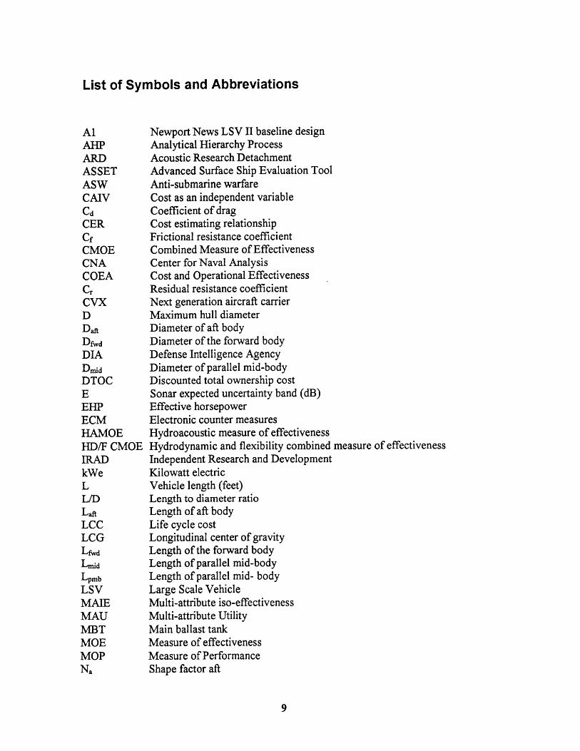
List of Symbols and Abbreviations
AlAHPARDASSETASWCAIVCdCERCfCMOECNACOEACrCVXDDaftDfwdDIADmidDTOCEEHPECMHAMOEHD/F CMOEIRADkWeLL/DLaftLCCLCGLfwd
Lmid
Lpmb
LSVMAIEMAUMBTMOEMOPNa
Newport News LSV II baseline designAnalytical Hierarchy ProcessAcoustic Research DetachmentAdvanced Surface Ship Evaluation ToolAnti-submarine warfareCost as an independent variableCoefficient of dragCost estimating relationshipFrictional resistance coefficientCombined Measure of EffectivenessCenter for Naval AnalysisCost and Operational EffectivenessResidual resistance coefficientNext generation aircraft carrierMaximum hull diameterDiameter of aft bodyDiameter of the forward bodyDefense Intelligence AgencyDiameter of parallel mid-bodyDiscounted total ownership costSonar expected uncertainty band (dB)Effective horsepowerElectronic counter measuresHydroacoustic measure of effectivenessHydrodynamic and flexibility combined measure of effectivenessIndependent Research and DevelopmentKilowatt electricVehicle length (feet)Length to diameter ratioLength of aft bodyLife cycle costLongitudinal center of gravityLength of the forward bodyLength of parallel mid-bodyLength of parallel mid- bodyLarge Scale VehicleMulti-attribute iso-effectivenessMulti-attribute UtilityMain ballast tankMeasure of effectivenessMeasure of PerformanceShape factor aft
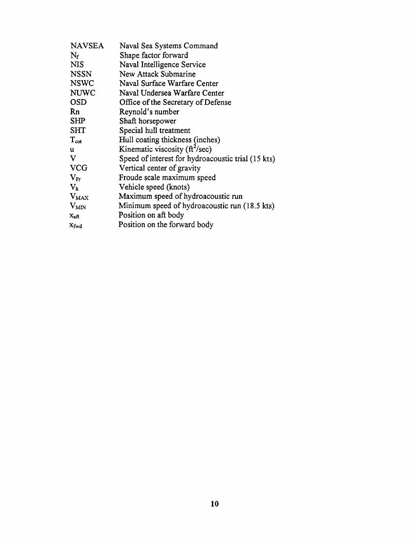
NAVSEANfNISNSSNNSWCNUWCOSDRnSHIPSHTToot
VVCGVFr
Vk
VMAX
VMIN
Xaft
Xfwd
Naval Sea Systems CommandShape factor forwardNaval Intelligence ServiceNew Attack SubmarineNaval Surface Warfare CenterNaval Undersea Warfare CenterOffice of the Secretary of DefenseReynold's numberShaft horsepowerSpecial hull treatmentHull coating thickness (inches)Kinematic viscosity (ft 2/sec)Speed of interest for hydroacoustic trial (15 kts)Vertical center of gravityFroude scale maximum speedVehicle speed (knots)Maximum speed of hydroacoustic runMinimum speed of hydroacoustic run (18.5 kts)Position on aft bodyPosition on the forward body
1Introduction
1.1 Background
The design of any complicated system is difficult because of the many trade-offs
required between cost and effectiveness. For example, in the automobile industry,
vehicle performance in terms of mileage and acceleration can be improved with the use
of lighter aluminum or polymer composite parts instead of steel. Most manufactures use
steel, however, because of the relatively low cost of steel fabrication. It is significantly
less expensive to produce steel cars, and most consumers are currently not willing pay the
premium for the increased performance.
Trade-offs must also be made between different measures of effectiveness. In
general, lower weight automobiles have better fuel economy and acceleration, but have
worse performance in crash-worthiness. Often government regulations can pit different
measures of effectiveness against each other. The Federal Motor Vehicle Safety
Standards dictate minimum crash-worthiness while the Environmental Protection Agency
emissions regulations dictate minimum fuel economy. The designer is left to develop a
balanced design that meets all requirements and provides vehicle performance at a price
the consumer is willing to pay while maximizing profit for the company. [1]
There are many examples of complicated design problems that have an infinite
number of possible options. Designers need tools that allow a structured search of the
design space with automatic evaluations of effectiveness and cost to determine the best
designs.
The problem is even more complicated if there are multiple objective attributes,
especially if they have no numeric value associated with them. An objective attribute is
any parameter that is optimized in a design problem. The only objective attribute for the
automobile manufacturer is some measure of profit as a return on investment. To obtain
an estimate of profit, however, the manufacturer must predict how many vehicles will be
sold. This is by no means an easy task, but clearly, the number of vehicles sold depends
upon the vehicle's perceived effectiveness and cost. Effectiveness depends upon safety,
cargo carrying capability, comfort, overall vehicle attractiveness, etc. Cost to the
consumer depends on purchase price, fuel cost, maintenance cost, resale value, etc. To
further complicate the problem, each of the high level measures of effectiveness depends
upon many lower level measures of effectiveness or measures of performance. For
example, comfort depends upon NVH (noise, vibration and harshness), legroom,
headroom, quality of seats, steering wheel adjustments, etc.
To solve the design issues of design space search and difficult-to-compare
measures of effectiveness, this thesis proposes the use of an evolutionary program with
expert opinion to develop a complete set of non-dominated designs, or Pareto frontier. A
design is non-dominated if no other possible design performs better in all objective
attributes. Expert opinion is used to combine the many measures of effectiveness into
several combined measures of effectiveness. This allows combination of similar items
that can more easily be compared by the decision-maker. Two methods of obtaining
expert opinion are explored: Analytical Hierarchy Process (AHP) and Multi-Attribute
Iso-effectiveness (MAIE).
1.2 Evolutionary Programs
The evolutionary program allows an effective search of the potential design space.
The expert opinion determines what constitutes a good design and the evolutionary
program searches the design space to determine which potential designs attain those
objectives. The evolutionary program is based on the principles of heredity and evolution
found in nature. A population of individual designs is randomly chosen and represented
in a binary string called a chromosome. Each individual in the population is evaluated
for its objective attributes (i.e., measures of effectiveness and cost). A new population is
formed by selecting the more fit individuals for reproduction to produce children.
Random mutations occur in the process to simulate mutations that occur in nature [2].
Individuals with poor objective attributes are chosen for removal from the population.
Over many generations, the program converges to a set of designs that represents the
non-dominated frontier of designs. If the true non-dominated (or Pareto) frontier is
found, then there is no design that has a better objective attribute without another
objective attribute having a worse value. [3]
1.3 Large Scale Vehicle II
The method proposed in this thesis is applied to Large Scale Vehicle II (LSV 11),
"an advanced, autonomous," large-scale submarine model "which will provide a platform
for fundamental research and development". LSV II will operate at the Acoustic
Research Detachment facility at Lake Pend Oreille, Idaho and "provide a platform for
evaluating new technologies for improvements in acoustics, propulsion, and
hydrodynamics". [4]
LSV I, currently operating at the Acoustic Research Detachment Facility, was
constructed to evaluate the propulsor on USS Seawolf (SSN-21). Several different
propulsor designs were evaluated before the selection of the final variant was chosen.
LSV I will remain operational until LSV II is completed. Consideration was given to
upgrading LSV I with an improved sensor system and hull coating, but was rejected
because of lack of arrangeable volume available for a trim tank. LSV I does not currently
have hull coating and has only small trim tanks. Because the coating compresses as the
vehicle dives, large trim tanks are required and LSV I does not have enough volume
margin to add the required tanks. [5]
Other than the hull coating, the biggest difference between LSV I and II is the
requirement for LSV II to support hydrodynamic testing. No hydrodynamic testing is
conducted with LSV I. [5]
The evaluation of fitness of each LSV II includes two measures of effectiveness
and one measure of cost. The hydroacoustic measure of effectiveness (HAMOE) is a
single calculated value that represents expected uncertainty in acoustic measurement.
The hydrodynamic and flexibility combined measure of effectiveness (HD/F CMOE) is
an expert opinion combination of three measures of performance. Discounted Total
Ownership Cost (DTOC) is used as the measure of vehicle cost.
LSV II is used as a platform for application of the proposed method because it is a
simplified design, yet representative of a full-scale ship or submarine design problem.
There is only one internal level on the vehicle, so the arrangement problem is simplified
to a linear stack of the required components. There are no crew members on board so
there is no human support problem. The detailed design problem of control of an
autonomous vehicle is more difficult. For the concept design of this analysis, however, it
is assumed that the control system is similar for all vehicles, carrying the same cost and
similar performance.
Naval ships and submarines are among the most complex systems ever designed.
A tool that assists the designer in determining the Pareto frontier would be of great value.
It is proposed that the method used in this thesis can be extended to the more complex
design problem of a full-scale ship or submarine with only minor changes.

(This page intentionally blank.)
2Previous and Current Methods for Concept Ship Design
A study is made of the methods used for concept ship design for the New Attack
Submarine (NSSN), next generation aircraft carrier (CVX) and the design method for
LSV II.
2.1 NSSN
Concept level design decisions for the New Attack Submarine were made in a two
phase Cost and Operational Effectiveness Analysis (COEA). The first phase was
completed in July of 1993 and the second phase was completed in May of 1995. [6,7]
2.1.1 COEA Phase I
Phase I of the COEA was conducted by the Center for Naval Analysis (CNA)
with technical assistance from Naval Sea Systems Command (NAVSEA) for design
information and cost estimates. All designs were conducted using a parametric
characteristic analysis. Cost was evaluated with a parametric analysis of life cycle cost
using a discount rate of 4.5%. Within Phase I, two separate analyses were conducted.
The goal of the first part of Phase I was to narrow the focus from 12 initial designs to a
smaller number of designs for further evaluation. Each of the 12 designs was evaluated
in 3 different scenarios at a rough order of magnitude. The scenarios were initially
dictated in general terms, from which Naval Intelligence Service (NIS) generated the
order of battle.' Naval Surface Warfare Center (NSWC) evaluated minefield penetration
1 Order of battle is a detailed description of opponents' forces including ships, submarines, aircraft, troops, etc.
ability, and Naval Undersea Warfare Center (NUWC) used SIM II2 to evaluate search
effectiveness and exchange ratio in combat against a variety of opponents. The
performance of each design was graded in each scenario to obtain a mission analysis
score and force on force analysis score. In the terminology of this paper, these are
measures of effectiveness. The scores were plotted versus cost to analyze cost-
effectiveness. [6]
The first part of Phase I concluded that there are 3 design discriminants that
dictate submarine effectiveness. Design discriminants are inherent ship characteristics
that have a large impact on effectiveness and cannot be easily changed after the ship is
constructed. The three design discriminants are stealth, speed and payload. In the
terminology of this paper, design discriminants are referred to as measures of
performance. It was decided that 4 of the 12 designs met the required design
discriminants at acceptable cost and were carried forward to the second part of Phase I.
[6]
During the second part of Phase I, a more detailed analysis was conducted for the
4 best designs. The same 3 scenarios were used, but more data was collected on the
performance of each variant in order to determine which of the 4 final selections would
be carried forward for more design work. At the end of the second part of Phase I, the
winning design was the nuclear attack submarine with "Seawolf-like" quieting, 28+ knots
of speed, four 21 inch torpedo tubes and 12 vertical launch cells. [6]
2 SIM II is a Monte Carlo based engagement model that predicts the performance of proposed submarines in variouswar scenarios.
Results from Phase I of the COEA were met with some criticism. Some members
of the Defense Intelligence Agency (DIA) thought that the wrong scenarios had been
used and that the order of battle for the enemy was incorrect. Similarly, individuals in the
Office of the Secretary of Defense (OSD) thought that more submarine variants should
have been evaluated. Since DIA and OSD had an official role in reviewing the COEA
results, this presented a major problem for the program office. [8]
2.1.2 COEA Phase II
A second COEA was commissioned to study the effects of varying design
parameters from the baseline design found in Phase I. From the beginning of Phase II, all
of the reviewers and decision makers were invited and encouraged to be involved in the
process as full members of the COEA team. Consensus was obtained in the scope and
assumptions of the study, including variant options, scenarios and orders of battle.
Obtaining consensus on the scope of Phase II of COEA was not easy, but the process
gave all people involved an investment in the analysis that yielded more credibility in the
results. [8]
The baseline ship for all variants was a nuclear attack submarine with Seawolf-
like stealth, 25,000 SHP, 28+ knots, 7500 tons submerged displacement, four 21-inch
torpedo tubes and 12 vertical launch cells. From this baseline a sensitivity analysis was
conducted by adding each of the following items and the evaluating effects on the major
warfare areas:
Light Weight Wide Aperture Array (LWWAA)Vertical Launch Cells (0, 4, 8, 12, 20)Special Hull Treatment (SHT)Chin Sonar ArrayLock Out Chamber (3, 6, and 9 team size)

Two types of towed arrays3" and 6.25" Counter Measures
Measures of effectiveness were selected to evaluate each platform's war-fighting
performance in the 7 mission areas:
Covert strikeAnti-submarine warfareCovert intelligence collectionAnti-surface warfareSpecial warfareMine warfareBattle group support
Each variant was placed in an operational context with a defined threat and
environment. The scenario was then executed and the MOE in each war-fighting area
determined. Measures of effectiveness in each war-fighting area were plotted as a
function of cost. The decision-maker was presented with these graphs in order to make a
final decision on the final variant. [7]
The COEA process was able to find the best variant in the design space that was
evaluated, but the design space that was compared was very small. Phase I of the COEA
looked at only 12 different variants and the Phase II looked at relatively small changes
around the variant determined to be best from Phase I. There is no guarantee that the
final variant found is the best of all possible in the design space. Hopefully, the designers
working on the project were able to design a submarine with effectiveness that is near the
optimum. A design tool that could assist with this process is needed.
2.2 CVX
Concept studies for the next generation of aircraft carrier were started in 1996 and
are planned to be completed by 2000. The CVX team is using a multi-step decision
process similar to the two phase COEA for NSSN. Unlike New Attack Submarine,

however, CVX plans to conduct more analysis separate from the congressionally
mandated studies. [9]
The COEA has been replaced by an Analysis of Alternatives (AOA) for CVX.
Essentially the purpose of the AOA is identical to that of the COEA, using a different
name. Phase I of the AOA, completed in 1997, was designed to select the size and
composition of the airwing. This study was similar in design and execution to Phase I of
the New Attack COEA. Parametric carrier designs were evaluated in combat scenarios to
determine effectiveness. Airwing size and composition were varied and the design was
balanced using the Navy's computer program for parametric design, ASSET (Advanced
Surface Ship Evaluation Tool). The designs were then evaluated for effectiveness in war
scenarios as a function of airwing size and composition. The decision was made to
proceed with an airwing with between 60 and 80 aircraft because of the increased strike
performance of the larger airwings. OSD had concerns about the study methods and
reduced the minimum airwing size to 50 aircraft. [9]
The remaining portions of the concept design process focus on maximizing the "-
ilities." These can be thought of as groups of measures of effectiveness and measures of
performance (MOEs and MOPs). There are 8 "ilities":
CombatabilitySurvivabilitySustainabiltiyInteroperabilityFlexibilitySupportabilityMobilityAffordability
The CVX design team assumes these "ilities" to be independent of each other to a
first order of magnitude. Affordability (low cost) is assumed the most significant driver
of the problem and is directly related to all of the other "ilities". [9]
The CVX team is currently in the process of defining MOEs and MOPs that can
be used to quantify each of the "ilities". The desire is to quantify effectiveness at four
different levels: campaign, mission, engagement and engineering. The campaign level
has 5 sub-levels ranging from pre-deployment through sustained combat. Each sub-level
has quantitative MOEs associated with it. For example, the proposed MOE for sustained
combat is target attrition. At the mission level, the performance of the carrier in a
specific mission area is evaluated. The mission areas include strike, anti-air warfare,
anti-surface warfare, anti-submarine warfare, self-defense, etc. At the engagement level,
different methods of employment are compared. At the engineering level, specific
systems are compared. In the mission area of self-defense, active and passive self-
defense measures are traded. At the engagement level under self-defense, active chaff
can be compared to active ECM (Electronic Counter Measures). And at the engineering
level under self-defense, different active ECM systems using different frequency bands
can be compared. [9]
Four levels are used because decision-makers at different levels within the design
team have different requirements for information. The engineering team working on the
design of the active ECM system may need to only have information comparing different
types of ECM performance. OSD, however, is primarily concerned with integration of
the new carrier into national defense at a very high level, and would be mostly interested
in the campaign level. [9]
The information for each level or sub-level is presented on a four-dimensional
plot. Each of the three axes represents one of the MOEs at this level, and the fourth
dimension is represented by color shading on the plot and represents affordability (cost).
The options that give the best cost-effectiveness at each level are passed to the next
higher level for further evaluation. [9]
Ultimately, MOEs as measured in required mission scenarios, cost and risk are the
critical objective attributes. MOPs determine MOEs, and design parameters determine
MOPs, cost and risk. MOPs and design parameters are not objectives unto themselves.
[13] Although the CVX design team confuses these basic concepts, at least it attempts to
quantify all aspects of the problem in order to make a definitive cost-effective decision.
2.3 LSV II
The Large Scale Vehicle II (LSV II) was proposed as a replacement for LSV I to
continue propulsor acoustic evaluation and research. LSV II is also being designed to
conduct hydrodynamic research. The program is under severe acquisition cost limitations
and is using cost as an independent variable (CAIV) to maintain costs within budget.
Since LSV II will be a one-of-a-kind vehicle, engineering costs cannot be spread over the
cost of several vehicle purchases. Maintaining engineering costs as low as practicable is
an even larger concern than on most acquisition projects. For this reason, as much as
possible, design work from LSV I is being used for LSV II. This initially led to the
decision to build the hull to the same specifications as LSV I, a Seawolf geo-similitude
model. When additional funds were budgeted for LSV II, the decision was made to
reconsider New Attack geo-similitude, since acoustic information on Seawolf had already
been gathered with LSV I. Very little study was given to any other geo-sim because of
the cost constraints on the program. The Seawolf geo-sim was under consideration for
maximum cost savings to the LSV program. The New Attack geo-sim was chosen
because additional funding was authorized specifically to build a New Attack geo-sim to
save model-testing costs for New Attack. [5]
Another major cost constraint on the program was the choice of the propulsion
motor. In order to meet the budget, the motor selected was the Electric Boat Radial Gap
Permanent Magnet Motor that was developed under Electric Boat's Independent
Research and Development (IRAD) program. [4]
Because of the various constraints placed on the LSV design by forces outside of
the program, it is difficult to compare the LSV concept design process to other methods.
2.4 Comparison with Proposed Method
The concept design decision tools used by NSSN and CVX both have several
similarities with the method proposed in this thesis. In all of the methods, a design is
evaluated for cost and effectiveness, and the designs are compared to find the optimal
solution for the final design. The important item missing from both previous methods is
a structured method to search design space to ensure that the decision-maker is selecting
from among the over-all non-dominated designs. Evolutionary programs can provide this
structure.

General Process
3.1 Overview
Designing a ship is very a complicated and involved process with a very large
number of interrelated design parameters. All design processes attempt to determine
which of the possible combinations are the best. The major hurdles to overcome in any
multi-objective design process are:
1. Selection of design parameters.
2. Determination of objective attributes (effectiveness and cost).
3. Selection of the best designs (those not dominated by other designs).
4. Final selection from among the non-dominated designs.
The determination of design effectiveness and cost can be very computationally
intensive and has traditionally required significant involvement of the ship designer.
Because each design has required such a significant amount of effort, only a small
fraction of the possible designs have traditionally been evaluated. This thesis proposes
automating the design process so that a computer model can evaluate designs from
selection of design parameters through determination of the non-dominated designs. The
designs to be evaluated are chosen through the use of an evolutionary program that treats
a group of designs as a biological population that evolves to the best possible designs.
The designs with the best objective attributes are chosen to reproduce, while the ones
with the worst objective attributes are removed from the population. The non-dominated
frontier can be defined using this method by evaluating only a fraction of all possible
designs.
3.2 Design Parameters
Design parameters are those physical characteristics of the proposed solution that
are varied in an attempt to obtain the best effectiveness at the least cost. They are the
smallest building block in concept ship design. Design parameters are grouped to form
potential designs. The designs are then balanced and evaluated for feasibility. Design
parameters include such characteristics as size, shape, material, subsystems, equipment,
etc. Most design parameters have competing effects on the overall effectiveness of a
final design. For example, in Large Scale Vehicle, adding hull coating lowers the
acoustic signature of the vehicle, but it also reduces the vehicle maximum speed and
increases cost. Maximum speed is lowered for two reasons:
1. Drag is increased due to more wetted surface area.
2. The trim tank must be sized to compensate for compression of the hull
coating. A larger trim tank uses internal volume that could otherwise be used
for more battery cells.
Without analyzing a wide range of coating thickness it is extremely difficult, if
not impossible, to determine the optimum thickness. The total impact of each design
parameter on the ship design must be evaluated.
When combined with all of the other design parameters, the number of possible
designs grows exponentially. Even with a simplified design analysis of LSV II using
only 8 design parameters, the number of possible designs is in the millions. With a full-

scale ship design, the number of possible combinations can easily number in the billions
or trillions.
3.3 Effectiveness and Cost
Many potential combinations of design parameters are not feasible for a number
of reasons: instability, lack of volume or area balance, lack of weight balance, etc. Of the
feasible designs, only a small fraction are non-dominated. A design is dominated if
another design performs at least equally well in all objective attributes and better in at
least one. For example, it does not make sense to choose a design with a higher cost if all
of the measures of effectiveness are the same.
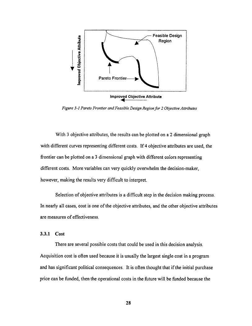
Each set of design parameters maps to a set of objective attributes which defines
the non-dominated or Pareto frontier. This frontier can be plotted in two or more
dimensions for assessment by the decision-maker. (See Figure 3-1.) In theory, the
number of objective attributes that can be compared in the Pareto frontier is not limited.
In practice, however, limiting the number of objective attributes to 3 or 4 simplifies
presentation of the information to the decision-maker. Any more than 3 or 4 is very
difficult to evaluate. In this thesis, the number of decision variables is limited to 3:
1. Discounted Total Ownership Cost
2. Hydroacoustic Measure of Effectiveness
3. Hydrodynamic/Flexibility Combined Measure of Effectiveness
- r-easIDIe uesignRegion
I
a Pareto Frontier
Improved Objective Attribute
Figure 3-1 Pareto Frontier and Feasible Design Region for 2 Objective Attributes
With 3 objective attributes, the results can be plotted on a 2 dimensional graph
with different curves representing different costs. If 4 objective attributes are used, the
frontier can be plotted on a 3 dimensional graph with different colors representing
different costs. More variables can very quickly overwhelm the decision-maker,
however, making the results very difficult to interpret.
Selection of objective attributes is a difficult step in the decision making process.
In nearly all cases, cost is one of the objective attributes, and the other objective attributes
are measures of effectiveness.
3.3.1 Cost
There are several possible costs that could be used in this decision analysis.
Acquisition cost is often used because it is usually the largest single cost in a program
and has significant political consequences. It is often thought that if the initial purchase
price can be funded, then the operational costs in the future will be funded because the
yearly operating and support expenditures are usually much smaller than the acquisition
cost and are funded from different sources. Over the life of the ship, however, these
operating and support costs typically sum to more money than the initial investment cost,
even when analyzed on a discounted basis.
Another potential cost is life cycle cost. Life cycle cost (LCC) is typically
defined as the sum of acquisition cost and direct operational and support cost over the life
of the program. Operating and support costs include direct expenditures for energy
consumption, manning, upgrades and maintenance. Indirect costs are not usually
included in life cycle costs. For example, the cost of paying the salary of the
maintenance workers is included, but the cost of any schooling required to train the
maintenance workers is not.
When all indirect costs are added to life cycle cost, total ownership cost (TOC) is
obtained. Total ownership cost can be very difficult to calculate because of the
uncertainty in how far it is appropriate to extend the indirect costs and the potential to
double count costs between programs. The effort expended in obtaining a correct cost
estimate is important, however, in properly defining the Pareto frontier.
A problem is encountered when using a TOC that is not discounted. In the non-
discounted case, a dollar spent in the first year is treated the same as a dollar spent at the
end of life. Since money has a time value associated with it, money spent in future years
should be discounted at an appropriate rate to present value. For this reason it is
important to use discounted TOC (DTOC). The Office of Management and Budget sets
the discount rate for the federal government. The discount rate for "public investment and
regulatory analyses" is currently set at 7%. Systems for the Department of Defense are
usually evaluated under "cost-effectiveness analysis", with a discount rate equal to the
real interest rates on Treasury Notes with a maturity equal to the period of concern. The
20-year discount rate is currently 3.7%. [10] Discount rates in the 1980's were set at
10%. This thesis uses a compromise discount rate of 6.0%.
Selection of the proper discount rate is extremely difficult, but also very
important. High discount rates discourage yearly expenditures and reward early savings,
while low discount rates encourage expenditures early in the program and reward savings
late in the program.
3.3.2 Measures of Effectiveness
Measures of effectiveness (MOEs) are functional metrics of a design relative to a
specific scenario. Measures of performance (MOPs) are functional metrics that have an
impact on the MOEs, but are not scenario dependent and are not the end result. [11] For
example, in the design of a warship, maximum speed is a MOP that is an input to a MOE
such as how many submarines the warship can sink. Having a high maximum speed
allows the ship to transit to the war zone more quickly allowing more effectiveness in
anti-submarine warfare and sinking of more submarines. The maximum speed is an
important factor, but it does not indicate directly how effective the platform is. To
determine effectiveness, the ship must be placed in a scenario. Evaluating MOPs
requires engineering models. Evaluating MOEs requires warfighting models.
As much as practical, the MOEs should be metrics that can be predicted using
computer models. In the anti-submarine warship example, war-game computer
simulation could be used to obtain the MOE metric. Perhaps exchange ratio (number of

submarines sunk to number of friendly ships lost) over an extended campaign, or series
of campaigns, is the desired MOE. For this thesis, one of the MOEs used is
hyrdroacoustic effectiveness, which depends upon the MOPs of vehicle speed and vehicle
endurance. The MOE also depends on the design parameters of hull coating thickness
and facility sonar type, which dictate acoustic performance of the system. The output
from the MOE is a calculated number that represents the expected uncertainty in
prediction of the propulsor acoustic performance of the vehicle. A smaller hydroacoustic
MOE indicates better effectiveness in this area.
3.3.3 Combined Measure of Effectiveness (CMOE)
A single number cannot always be chosen to reflect the effectiveness of a design
in a certain area. In the case of the anti-submarine example, perhaps it is important to
have separate numbers for deep water and littoral effectiveness. One option is to create
another category for comparison on the Pareto frontier. If the number of objective
attributes grows to more than 3 or 4, however, presenting the decision-maker with the
information becomes a problem. Another option is to use expert opinion to group 2 or
more MOEs into a combined measure of effectiveness (CMOE).
3.3.3.1 Previous CMOE Methods
Whitcomb [12] outlines several different methods to obtain this CMOE:
1. Weighted Sum
2. Hierarchical Weighted Sum
3. Analytic Hierarchy Process (AHP)
4. Multi-attribute Utility (MAU) Analysis

All of the methods used to obtain a CMOE have the first two steps in common.
The first step is to determine the attributes to be combined (MOEs or MOPs) to obtain the
CMOE. The next step is to establish goals and thresholds. Goals represent the best value
the decision-maker believes to be obtainable with the technology available in the time
frame of the project, or the value at which further improvement no longer adds significant
benefit to the project. The threshold represents the value of worst acceptable
performance. Below this value, it is considered not worth continuing the project. [13]
The weighted sum method is the simplest of these methods. The CMOE is
obtained by summing the product of the MOEs and their respective weightings. The
MOEs are weighted by the decision-maker according to the MOEs perceived importance.
This method has the advantage of simplicity, but its validity is highly dependent on a
clear and precise definition of the problem and a thorough understanding of this
definition by the expert. [14]
Hierarchical weighted sum is an extension of the weighted sum method with a
more structured approach to the problem. The top of the hierarchy is the CMOE. Below
this are the top-level measures of effectiveness. In the warship example, the top level
MOE is anti-submarine warfare. Below this are lower level MOEs, which in the example
are deep water ASW and littoral ASW. If the lowest level MOE cannot be numerically
evaluated, then the hierarchy can be broken down further into MOPs. For example, ASW
weapons, maximum speed, endurance, etc. all affect the ability for a warship to succeed
in an ASW mission. This method also uses expert opinion to obtain the relative
weightings of each level of the hierarchy, but complex problems are more easily handled
in the hierarchy structure, allowing the design team and the decision maker a format to
facilitate discussion. This method also has the benefit of simple implementation on any
spreadsheet program.
The Analytical Hierarchy Process (AHP) uses a hierarchy similar to the one used
for hierarchical weighted sum, but relies on the decision maker to make pairwise
comparisons as to the relative importance of each item within a level of the hierarchy.
The relative weightings for each comparison are then placed in a square matrix with row
and columns representing the elements of each sub-objective in the hierarchy. The
weights for each objective are the numbers within the eigenvector associated with the
largest eigenvalue. AHP is not as simple to implement as the first two methods, but with
the use of "Expert Choice" software [15], the process is fairly straightforward. The
number of elements compared at each node should typically be limited to no more than 7
to facilitate the decision makers ease of comparison. This is typically not a significant
problem; more branches can be added to the hierarchy if necessary.
Multi-attribute utility analysis involves obtaining the decision-maker's preference
or utility for certain levels of performance or effectiveness. A hierarchy is not required
for this method, but may be useful in formulation of the problem. Utility functions, if
generated properly, provide insight into the decision makers preferences for
effectiveness, performance, uncertainty and risk. The biggest drawback to the use of
MAU analysis is the difficulty in obtaining utility curves. The decision-maker is asked
questions dealing with the probability of certain outcomes of the designs. Decision-
makers are often not experienced with thinking about the probability of outcomes, and
experienced consultants are required to assist in creation of the utility curves. Another
drawback of the method is that the results are not obtained from the interviews directly,
but through a somewhat indirect mathematical method. The final utility curves can often
be non-intuitive, which can cause problems in group facilitation if there is more than one
decision-maker.
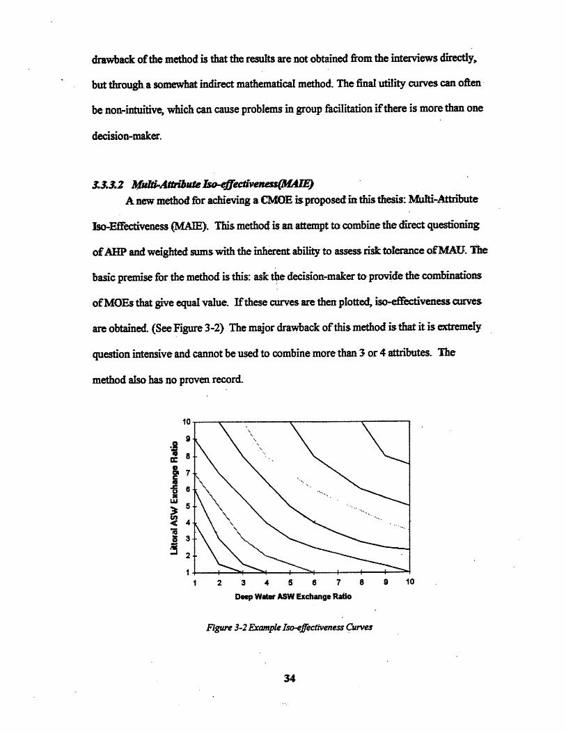
s33..2 M ti&AttriuteIso-effeclveness(M4IEA new method for achieving a CMOE is proposed in this thesis: Multi-Attribute
Iso-Effectiveness (MAE). This method is an attempt to combine the direct questioning
of AHP and weighted sums with the inherent ability to assess risk tolerance ofMAU. The
basic premise for the method is this: ask the decision-maker to provide the combinations
of MOEs that give equal value. If these curves are then plotted, iso-effectiveness curves
are obtained. (See Figure 3-2) The major drawback of this method is that it is extremely
question intensive and cannot be used to combine more than 3 or 4 attributes. The
method also has no proven record.
10
9
1 2 3 4 5 6 7 8 9 104-3-
Deep Water ASW Exchange Ratio
Figure 3-2 Example Iso-effectiveness Curves
34
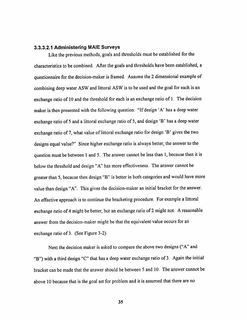
3.3.3.2.1 Administering MAlE Surveys
Like the previous methods, goals and thresholds must be established for the
characteristics to be combined. After the goals and thresholds have been established, a
questionnaire for the decision-maker is framed. Assume the 2 dimensional example of
combining deep water ASW and littoral ASW is to be used and the goal for each is an
exchange ratio of 10 and the threshold for each is an exchange ratio of 1. The decision
maker is then presented with the following question: "If design 'A' has a deep water
exchange ratio of 5 and a littoral exchange ratio of 5, and design 'B' has a deep water
exchange ratio of 7, what value of littoral exchange ratio for design 'B' gives the two
designs equal value?" Since higher exchange ratio is always better, the answer to the
question must be between 1 and 5. The answer cannot be less than 1, because then it is
below the threshold and design "A" has more effectiveness. The answer cannot be
greater than 5, because then design "B" is better in both categories and would have more
value than design "A". This gives the decision-maker an initial bracket for the answer.
An effective approach is to continue the bracketing procedure. For example a littoral
exchange ratio of 4 might be better, but an exchange ratio of 2 might not. A reasonable
answer from the decision-maker might be that the equivalent value occurs for an
exchange ratio of 3. (See Figure 3-2)
Next the decision maker is asked to compare the above two designs ("A" and
"B") with a third design "C" that has a deep water exchange ratio of 3. Again the initial
bracket can be made that the answer should be between 5 and 10. The answer cannot be
above 10 because that is the goal set for problem and it is assumed that there are no

solutions above this value. The answer cannot be less than 5, because if it were, then
design "A" would be better in both categories and have a higher value. Again the
bracketing procedure can be performed and a reasonable answer might be 7. The deep
water ASW exchange ratios are varied until the entire iso-effectiveness line is obtained.
The questions then start over to define another iso-effectiveness line. For
example, the first design on the next iso-effectiveness curve might have both exchange
ratios equal to 3. The process is repeated until the entire grid is populated with iso-
effectiveness curves.
The slopes of these curves represent the relative value of deep water ASW to
littoral ASW. In regions where the slope is near 1, deep water and littoral ASW have
close to the same value. In regions where the curves are very steep, deep water ASW is
more valuable. In regions where the curves are very flat, littoral ASW is more important.
To extend the method to a third dimension, the assumption is made that the iso-
effectiveness curves obtained for two dimensions are not dependent upon the third
dimension. The decision-maker is told to hold the third variable constant while
developing the iso-effectiveness curves for the first two. Another set of iso-effectiveness
curves is then obtained for the third variable and one of the first two variables. These two
sets of iso-effectiveness curves are then combined to form iso-effectiveness surfaces.
Cross sections of these surfaces perpendicular to one of the variable axis yield iso-
effectiveness curves of the remaining two variables.
In theory, this process can be extended to more dimensions, but the number of
questions required to obtain the iso-effectiveness curves increases rapidly with increasing

numbers of variables. If the number of points required to find a 2-dimension iso-
effectiveness curve is P (typically between 10 and 30) and the number of variables is N,
then the total number of points that must be evaluated is:
Number of Points = P * (N-1)
3.3.3.2.2 Interpreting MAIE Surveys
The CMOE for a set of objective attributes described by an iso-effectiveness
curve (surface) is the intersection of the iso-effectiveness curve (surface) of the attributes
under consideration with the vertical axis. The CMOE for the 2 dimensional example is
the value of the independent variable at the location of the threshold value of the
dependent variable along the iso-effectiveness curve on which the point of interest lies.
For example, in Figure 3-1, if the deep-water exchange ratio is 5 and the littoral exchange
ratio is 3, the point plots on an iso-effectiveness curve. When this iso-effectiveness curve
is traced to the point where it crosses the threshold value for deep-water exchange ratio
(1), the CMOE is found to be 9. If the deep-water exchange ratio is 5 and the littoral
exchange ratio is 2.25, the point plots halfway between two iso-effectiveness lines.
These two curves intersect the vertical axis at 7 and 9, so the CMOE is 8.
If the iso-effectiveness curve does not intersect the dependent variable axis, then
the CMOE is obtained by extrapolating the iso-effectiveness curve to the dependent
variable axis. Note that this yields a number greater than the goal for the dependent
variable. The CMOE does not represent the actual value obtained in the independent
variable space; it merely gives a relative value of the effectiveness of the combination of
variables.
The process in 3 dimensions is similar, but instead of interpolating iso-
effectiveness curves, iso-effectiveness surfaces are interpolated. The variable that is used
to obtain both sets of iso-effectiveness curves is the independent variable that is used to
express the CMOE. The CMOE is the value of the independent variable on the iso-
effectiveness surface where the values of the dependent variables are equal to the
threshold value. A specific example of the 3-dimension application to LSV is presented
in Chapter 4.
3.4 Evolutionary Program
Once objective attribute functions or models are defined, the task remains to
obtain the Pareto frontier: those designs that cannot be improved in one objective
attribute without sacrificing another objective attribute. Of the large number of potential
designs, only a small fraction are typically non-dominated. For simple designs, it may be
possible to evaluate all of the possible combinations of design parameters and determine
all of the non-dominated designs. For more complex design problems, however, the
exhaustive search method is not feasible because it takes too long to complete the
evaluation. Some sort of optimization program must be used to obtain the Pareto frontier.
This thesis proposes the use of an evolutionary program.
3.4.1 Evolutionary Program Background
An evolutionary program treats an individual design as a member of a biological
population. The members of the population with design parameters that map to the most
dominant objective attributes are chosen to mate and produce offspring. The members of
the population with dominated objective attributes are removed. After many generations
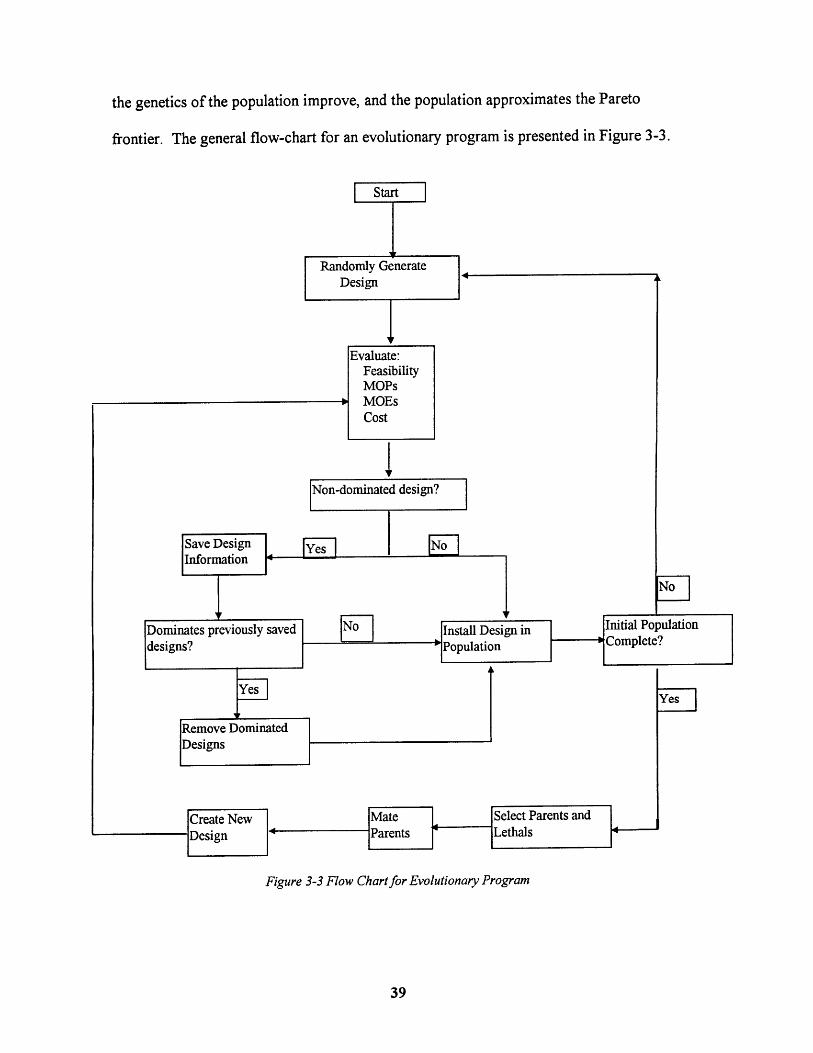
the genetics of the population improve, and the population approximates the Pareto
frontier. The general flow-chart for an evolutionary program is presented in Figure 3-3.
Figure 3-3 Flow Chart for Evolutionary Program
The theory behind evolutionary programs is currently uncertain and controversial.
Experimental results indicate that the process shows promise in optimizing solutions,
especially for "ill-behaved" problems when discontinuous or disjoint functions are
present. There has been a significant amount of research about optimizing single
objective attribute problems, but relatively little in the area of multi-objective attribute
problems. Evolutionary programs to optimize Pareto frontier problems are even less well
documented. [3]
Evolutionary programs have the advantage that they are simple to implement.
They can readily be applied to many optimization problems in a straightforward method.
The process is easy to understand because it is intuitive in its application. [3]
Another advantage of the method is that it provides a good combination of
exploration and exploitation of the design space. Exploration ensures that no areas of the
design space are ignored, while exploitation implies that solutions with good fitness are
used to further increase fitness. Some other search methods can focus prematurely
around local optimums found early in the search process, perhaps missing a global
optimum. Evolutionary programs tend not to have this problem. They use the
information that is contained in the genetics to exploit local optimums, while still
exploring the entire search space, especially through mutations. [3]
A major disadvantage of an evolutionary program is the lack of formal proof
about why the algorithm works. There is some research that suggests that for certain
problems other types of search engines work better. Because of the lack of formal theory
and mathematical proofs, the best method to set up an evolutionary program is not fully

understood. The best method seems to be to set up the problem, and then vary the
evolutionary program parameters until the algorithm is operating effectively. [2,3]
3.4.2 Binary Representation
A binary string called a chromosome represents each potential design. The
chromosome is composed of genes that represent individual design parameters. The
genes can represent either discreet or continuous variables.
For discreet variables, it is advantageous to force the number of options for the
variable to be of the form 2N, where N represents the gene length. This simplifies the
representation because each gene is a binary string that represents 2 possible
combinations. If the number of options for a discreet variable is not of the form 2N, then
2 or more chromosomes can be combined to represent the variables. Alternatively,
values of the gene can be made infeasible. If these values are generated in the
evolutionary algorithm, then the design is not evaluated. This thesis uses 2 discreet
variables: battery type, which has 4 options and sonar type, which has 2 options.
Continuous variables are represented in the binary strings as discreet variables.
The separation between the variable values depends on the length of the gene chosen. A
gene that has only one binary digit can represent only the minimum and maximum
variable values. The total number of values that can be represented is 2 raised to the
number of binary digits in the gene. The separation between the variable values is:
Value , - Value,Separation = 2- egt -12G~' -1
It is important to ensure that the chromosomes are long enough to provide enough
information so that large gaps are not created in the objective attribute space. However,
it is also important not to make the gene too long, as each binary digit added to the
chromosome doubles the number of possible designs. A good approach is to start with
chromosomes slightly shorter than desired, and then, after the genetic algorithm is
operating correctly, increase the size of the chromosomes until the desired precision is
reached.
3.4.3 First Generation
The first generation of potential designs is created randomly. Each element of the
binary chromosome string is randomly assigned a value of"O" or "1". After the entire
chromosome has been generated, the design is decoded into a base-10 representation and
evaluated for feasibility, performance, effectiveness and cost. The process is repeated
until the first generation is fully populated.
The optimal size for the generation depends upon the individual design problem.
A larger population allows more genetic information to be available to the algorithm at
any given time, but a larger population also takes longer to generate new individuals,
especially if clones are prohibited in the population. Two designs are clones of each other
if all of the genetic information contained in the two chromosomes is duplicated exactly.
The algorithm used in this thesis does not permit clones. Clones add no new information
to the Pareto frontier so, in a multi-attribute decision problem, it is beneficial to prohibit
clones. If clones are allowed, then the members of the population may have a tendency
to gather around a few designs near the Pareto frontier and limit the number of other
designs found on the frontier.

3.4.4 Subsequent Generations
After the first generation, new designs (offspring) are created by mating designs
that possess dominant objective attributes. The offspring replace designs that possess
dominated objective attributes (lethals). There are several possible methods to select
parents and lethals, but only the tournament method is used and discussed. [3]
3.4.4.1 Selection
The tournament method randomly selects a fraction of the population to compete
in a tournament. Each contestant in the tournament is compared against all other
contestants to determine how many contestants dominate it.
If only one contestant is non-dominated, then it is declared the winner of the
tournament and goes on to become a parent. If more than one contestant is non-
dominated then the contestant with the lowest niche count is declared the winner. A
niche count is a count of the number of other contestants that are "close" to an individual
in objective attribute space. "Close" is a relative term that must be determined
experimentally. Small populations require larger niche sizes so that the designs will more
evenly spread over the Pareto frontier. Large populations can have smaller niche sizes
and still maintain an adequate spread over the Pareto frontier. If more than one non-
dominated contestant is tied for the lowest niche count, then the winner is chosen
randomly from the non-dominated, low niche count contestants. [3]
The loser of the tournament, which is removed from the population, is the
contestant that is dominated by the most contestants. If there is more than one most
dominated contestant, then the one with the highest niche count is the loser. If there is
still a tie, then the loser is selected randomly from among the most dominated, highest
niche count contestants. [3]
Two tournaments are held to select 2 parents and 2 lethals. After the second
tournament, the parents are compared and the lethals are compared to ensure that the
selections are not duplicates. If the same parent or lethal is selected, then the tournament
process is repeated until unique parents and lethals are found. [3]
Tournament size is variable in the genetic algorithm. A large tournament size
favors those members of the population that have good objective attributes in the current
generation. In early generations, however, there is a fairly high probability that the best
performers will not be the best performers in the later generations. To maintain genetic
diversity, it is desirable to maintain some characteristics from weaker members,
especially in early generations. At one extreme, if tournament size is set to the entire
population, then only the over-all non-dominated individuals of the population will go on
to reproduce, and it is possible that some valuable genetic information may be lost. At
the other extreme, if only 2 members of the population are selected as contestants, then
there is very little exploitation, and the search becomes nearly random.
3.4.4.2 Crossover
The parents selected from the tournament are mated using crossover to create 2
offspring. Each of the parents' chromosomes is cut at the same location. The location of
the cut is randomly chosen. The portion of the chromosome to the right of the cut is
swapped between the two parents to obtain two new offspring.
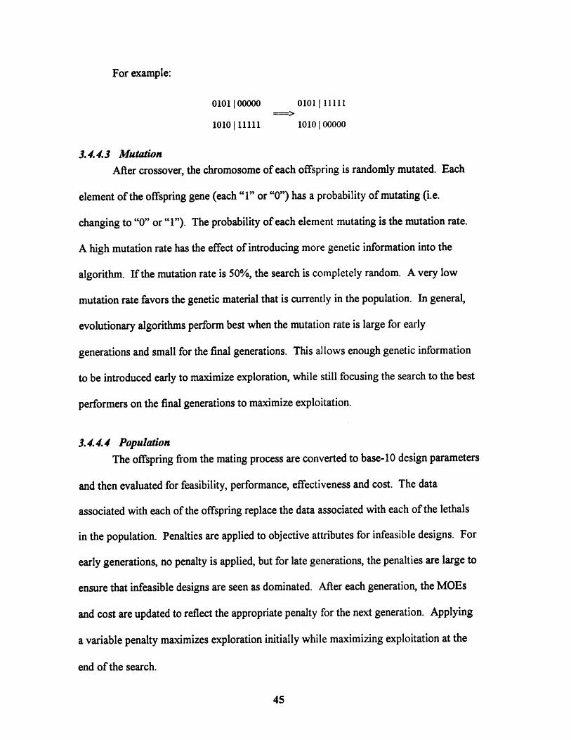
For example:
0101o00000 0101111111
1010 11111 1010oo 00000
3.4.4.3 Mutation
After crossover, the chromosome of each offspring is randomly mutated. Each
element of the offspring gene (each "1" or "0") has a probability of mutating (i.e.
changing to "0" or "1"). The probability of each element mutating is the mutation rate.
A high mutation rate has the effect of introducing more genetic information into the
algorithm. If the mutation rate is 50%, the search is completely random. A very low
mutation rate favors the genetic material that is currently in the population. In general,
evolutionary algorithms perform best when the mutation rate is large for early
generations and small for the final generations. This allows enough genetic information
to be introduced early to maximize exploration, while still focusing the search to the best
performers on the final generations to maximize exploitation.
3.4.4.4 Population
The offspring from the mating process are converted to base-10 design parameters
and then evaluated for feasibility, performance, effectiveness and cost. The data
associated with each of the offspring replace the data associated with each of the lethals
in the population. Penalties are applied to objective attributes for infeasible designs. For
early generations, no penalty is applied, but for late generations, the penalties are large to
ensure that infeasible designs are seen as dominated. After each generation, the MOEs
and cost are updated to reflect the appropriate penalty for the next generation. Applying
a variable penalty maximizes exploration initially while maximizing exploitation at the
end of the search.

3.4.4.4. Non-Dominated Designs
After each new design has been inserted into the population array, it is compared
to all previously found non-dominated designs. If the design is infeasible, it is never
saved as a non-dominated design. If a design is non-dominated, it is saved in the non-
dominated array. A check is then performed to determine if the newly found non-
dominated design dominates any of the designs already in the non-dominated array. If
any designs are now dominated, they are removed. A final check is made to determine if
the new design has the same MOEs and cost as a design that has already been found to be
non-dominated. If such a design is found, the design parameters are checked to
determine if the design is a clone or a new design. If it is a clone, it is rejected; if it is a
unique design, it is saved.
3.5 Presentation to the Decision-Maker
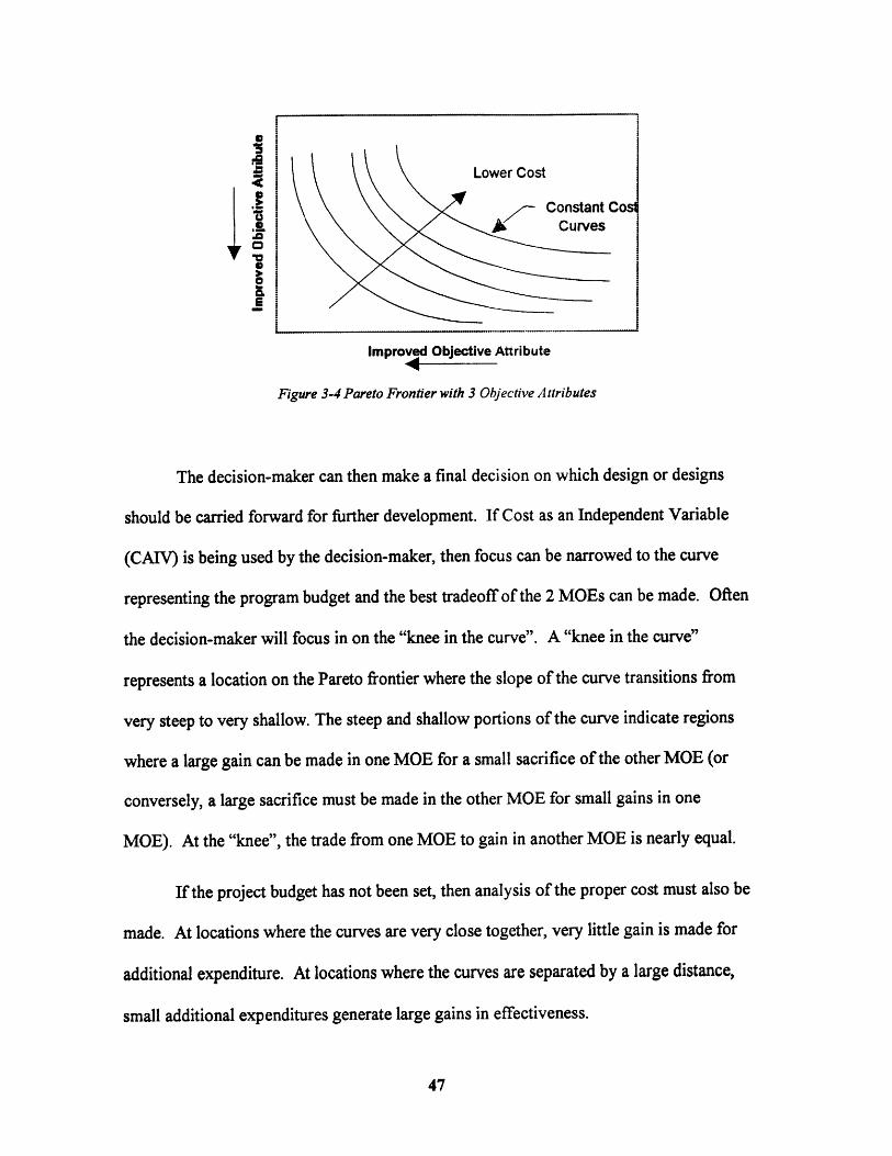
The decision-maker is presented with a plot that represents the Pareto frontier. If
two MOEs and cost are used as the objective attributes, then the horizontal and vertical
axis each represent one of the MOEs. The Pareto frontier is plotted for each cost of
interest. Each curve represents a different cost.
SLower cost01
S. ............ antCurves
Improved Objective Attribute4-
Figure 3-4 Pareto Frontier with 3 Objective Attributes
The decision-maker can then make a final decision on which design or designs
should be carried forward for further development. If Cost as an Independent Variable
(CAIV) is being used by the decision-maker, then focus can be narrowed to the curve
representing the program budget and the best tradeoff of the 2 MOEs can be made. Often
the decision-maker will focus in on the "knee in the curve". A "knee in the curve"
represents a location on the Pareto frontier where the slope of the curve transitions from
very steep to very shallow. The steep and shallow portions of the curve indicate regions
where a large gain can be made in one MOE for a small sacrifice of the other MOE (or
conversely, a large sacrifice must be made in the other MOE for small gains in one
MOE). At the "knee", the trade from one MOE to gain in another MOE is nearly equal.
If the project budget has not been set, then analysis of the proper cost must also be
made. At locations where the curves are very close together, very little gain is made for
additional expenditure. At locations where the curves are separated by a large distance,
small additional expenditures generate large gains in effectiveness.
No matter which design is finally chosen, however, this type of analysis provides
a set of designs that are not dominated by any other designs. The decision-maker is given
the opportunity to choose from among a group of non-dominated designs.
4Detailed Process
This chapter provides the detailed process proposed for LSV II multi-attribute
decision analysis. It is an application of the method proposed in Chapter 3.
4.1 Design Parameters
Design parameters are the vehicle's physical characteristics that are varied in an
attempt to maximize the effectiveness ofLSV II. Only the most important design
parameters are varied to demonstrate the proposed decision method. The goal is to
choose parameters that have the greatest impact on the effectiveness and cost of the
vehicle. For the purposes of this study, parameters are also chosen to ensure information
is available to analyze the effects of varying the parameters.
Design ParametersMaximum Hull Diameter (D)Length to Diameter Ratio (LID)Shape Factor Forward (N)Shape Factor Aft (N.)Battery TypeBattery SizeHull Coating ThicknessSonar Type
Maximum hull diameter is varied between 8 and 15 feet. The lower limit is
chosen to ensure that the electric propulsion motor chosen for the vehicle fits in the hull.
The upper limit is an estimate of the maximum feasible diameter due to limits on
handling equipment.
Length to diameter ratio is varied between 6 and 13. The lower limit is chosen
because drag is near a minimum near this ratio. The upper limit is chosen because
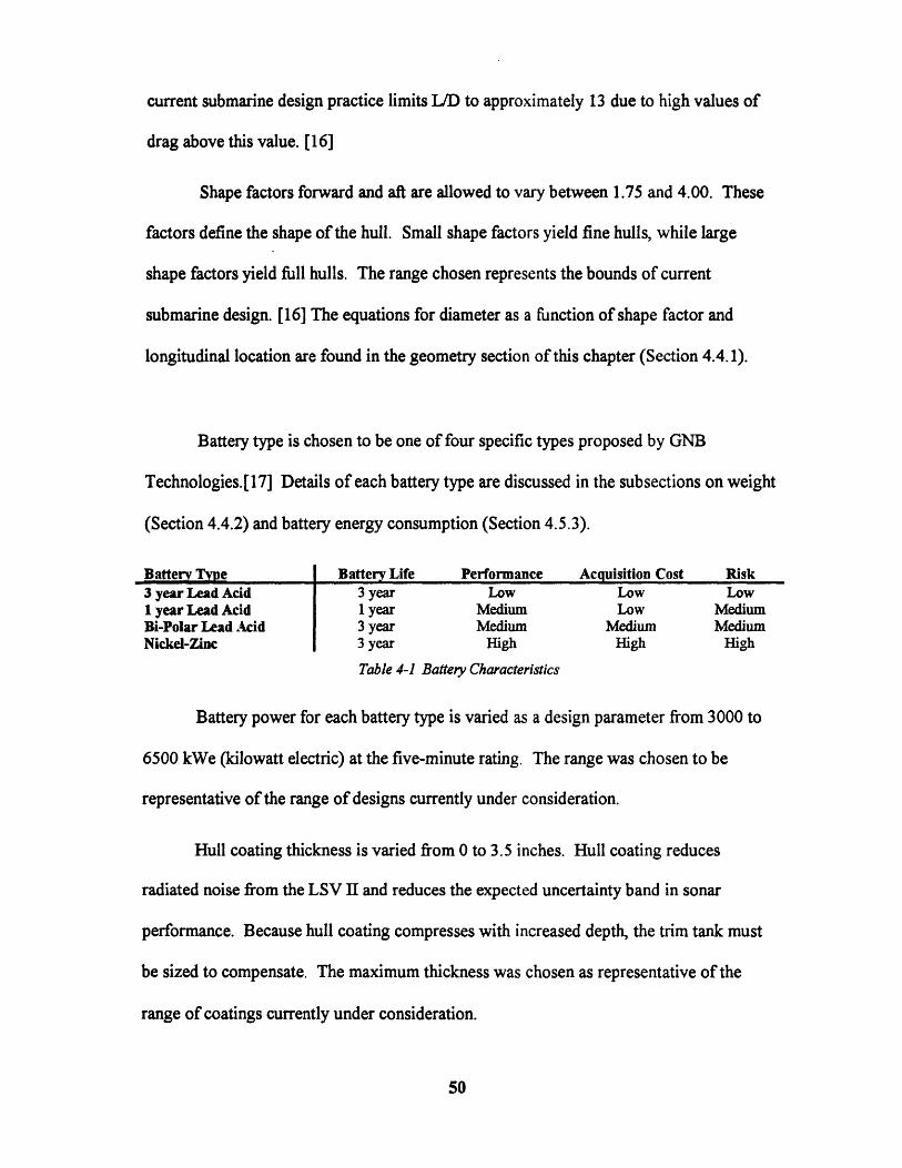
current submarine design practice limits L/D to approximately 13 due to high values of
drag above this value. [16]
Shape factors forward and aft are allowed to vary between 1.75 and 4.00. These
factors define the shape of the hull. Small shape factors yield fine hulls, while large
shape factors yield full hulls. The range chosen represents the bounds of current
submarine design. [16] The equations for diameter as a function of shape factor and
longitudinal location are found in the geometry section of this chapter (Section 4.4.1).
Battery type is chosen to be one of four specific types proposed by GNB
Technologies.[17] Details of each battery type are discussed in the subsections on weight
(Section 4.4.2) and battery energy consumption (Section 4.5.3).
Battery Type Battery Life Performance Acquisition Cost Risk3 year Lead Acid 3 year Low Low Low1 year Lead Acid 1 year Medium Low MediumBi-Polar Lead Acid 3 year Medium Medium MediumNickel-Zinc 3 year High High High
Table 4-1 Battery Characteristics
Battery power for each battery type is varied as a design parameter from 3000 to
6500 kWe (kilowatt electric) at the five-minute rating. The range was chosen to be
representative of the range of designs currently under consideration.
Hull coating thickness is varied from 0 to 3.5 inches. Hull coating reduces
radiated noise from the LSV II and reduces the expected uncertainty band in sonar
performance. Because hull coating compresses with increased depth, the trim tank must
be sized to compensate. The maximum thickness was chosen as representative of the
range of coatings currently under consideration.
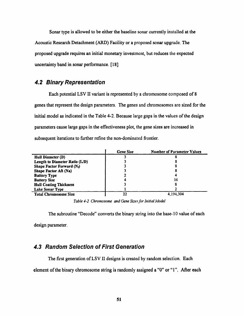
Sonar type is allowed to be either the baseline sonar currently installed at the
Acoustic Research Detachment (ARD) Facility or a proposed sonar upgrade. The
proposed upgrade requires an initial monetary investment, but reduces the expected
uncertainty band in sonar performance. [18]
4.2 Binary Representation
Each potential LSV II variant is represented by a chromosome composed of 8
genes that represent the design parameters. The genes and chromosomes are sized for the
initial model as indicated in the Table 4-2. Because large gaps in the values of the design
parameters cause large gaps in the effectiveness plot, the gene sizes are increased in
subsequent iterations to further refine the non-dominated frontier.
Gene Size Number of Parameter ValuesHull Diameter (D) 3 8Length to Diameter Ratio (L/D) 3 8Shape Factor Forward (Nf) 3 8Shape Factor Aft (Na) 3 8Battery Type 2 4Battery Size 4 16Hull Coating Thickness 3 8Lake Sonar Type 1 2Total Chromosome Size 22 4,194,304
Table 4-2 Chromosome and Gene Sizes for Initial Model
The subroutine "Decode" converts the binary string into the base- 10 value of each
design parameter.
4.3 Random Selection of First Generation
The first generation ofLSV II designs is created by random selection. Each
element of the binary chromosome string is randomly assigned a "0" or "1". After each
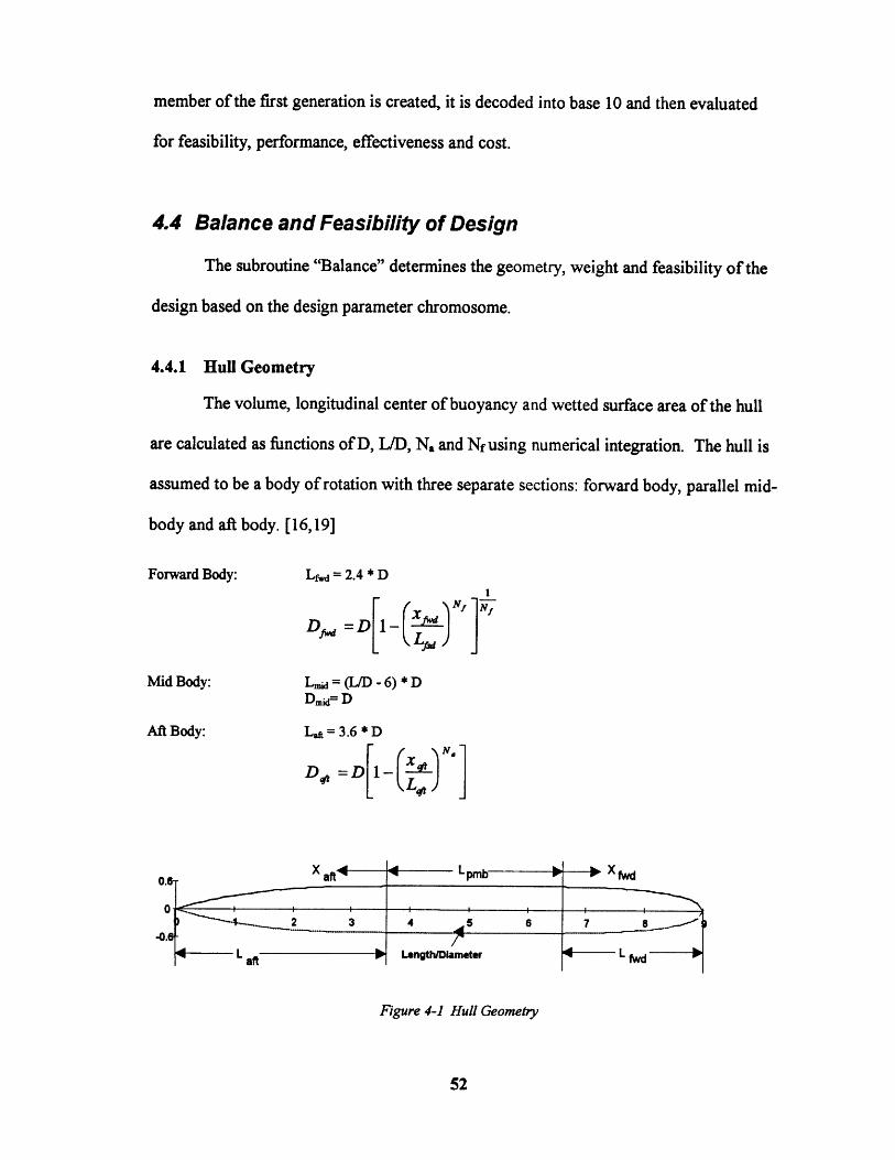
member of the first generation is created, it is decoded into base 10 and then evaluated
for feasibility, performance, effectiveness and cost.
4.4 Balance and Feasibility of Design
The subroutine "Balance" determines the geometry, weight and feasibility of the
design based on the design parameter chromosome.
4.4.1 Hull Geometry
The volume, longitudinal center of buoyancy and wetted surface area of the hull
are calculated as functions of D, L/D, Na and Nf using numerical integration. The hull is
assumed to be a body of rotation with three separate sections: forward body, parallel mid-
body and aft body. [16,19]
Forward Body:
Mid Body:
Aft Body:
Lfd = 2.4 * D1
Df = D 1-(- I
Lm, = (L/D - 6) * DDmi = D
L.& = 3.6 * D
D* =D 1- X-- L *t
Figure 4-1 Hull Geometry
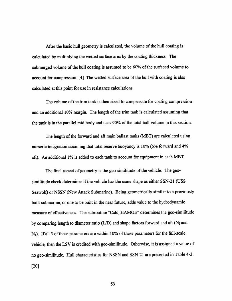
After the basic hull geometry is calculated, the volume of the hull coating is
calculated by multiplying the wetted surface area by the coating thickness. The
submerged volume of the hull coating is assumed to be 60% of the surfaced volume to
account for compression. [4] The wetted surface area of the hull with coating is also
calculated at this point for use in resistance calculations.
The volume of the trim tank is then sized to compensate for coating compression
and an additional 10% margin. The length of the trim tank is calculated assuming that
the tank is in the parallel mid body and uses 90% of the total hull volume in this section.
The length of the forward and aft main ballast tanks (MBT) are calculated using
numeric integration assuming that total reserve buoyancy is 10% (6% forward and 4%
aft). An additional 1% is added to each tank to account for equipment in each MBT.
The final aspect of geometry is the geo-similitude of the vehicle. The geo-
similitude check determines if the vehicle has the same shape as either SSN-21 (USS
Seawolf) or NSSN (New Attack Submarine). Being geometrically similar to a previously
built submarine, or one to be built in the near future, adds value to the hydrodynamic
measure of effectiveness. The subroutine "CalcHAMOE" determines the geo-similitude
by comparing length to diameter ratio (L/D) and shape factors forward and aft (Nf and
Na). If all 3 of these parameters are within 10% of these parameters for the full-scale
vehicle, then the LSV is credited with geo-similitude. Otherwise, it is assigned a value of
no geo-similitude. Hull characteristics for NSSN and SSN-21 are presented in Table 4-3.
[20]
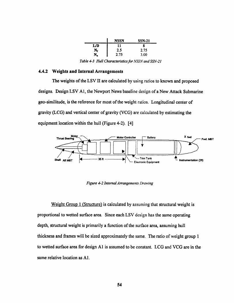
NSSN SSN-21L/D 11 8Nr 2.5 2.75N, 2.75 3.00
Table 4-3 Hull Characteristics for NSSN and SSN-21
4.4.2 Weights and Internal Arrangements
The weights of the LSV II are calculated by using ratios to known and proposed
designs. Design LSV Al, the Newport News baseline design of a New Attack Submarine
geo-similitude, is the reference for most of the weight ratios. Longitudinal center of
gravity (LCG) and vertical center of gravity (VCG) are calculated by estimating the
equipment location within the hull (Figure 4-2). [4]
M otor - Motor Controller Battery X Fwd. MBT
Shaft ATr MBT 35f Tim Tank Instrumentation (2ft)Shaft AElectronic Equipment Intrumentation (2ff)
Figure 4-2 InternalArrangements Drawing
Weight Group 1 (Structure) is calculated by assuming that structural weight is
proportional to wetted surface area. Since each LSV design has the same operating
depth, structural weight is primarily a function of the surface area, assuming hull
thickness and frames will be sized approximately the same. The ratio of weight group 1
to wetted surface area for design Al is assumed to be constant. LCG and VCG are in the
same relative location as Al.
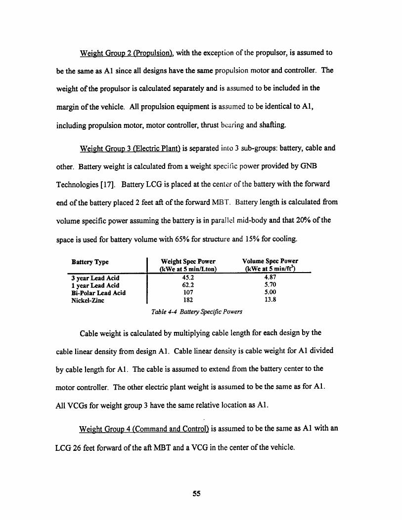
Weight Group 2 (Propulsion), with the exception of the propulsor, is assumed to
be the same as Al since all designs have the same propulsion motor and controller. The
weight of the propulsor is calculated separately and is assumed to be included in the
margin of the vehicle. All propulsion equipment is assumed to be identical to Al,
including propulsion motor, motor controller, thrust bearing and shafting.
Weight Group 3 (Electric Plant) is separated into 3 sub-groups: battery, cable and
other. Battery weight is calculated from a weight speci tic power provided by GNB
Technologies [17]. Battery LCG is placed at the center of the battery with the forward
end of the battery placed 2 feet aft of the forward MBT. Battery length is calculated from
volume specific power assuming the battery is in parallel mid-body and that 20% of the
space is used for battery volume with 65% for structure and 15% for cooling.
Battery Type Weight Spec Power Volume Spec Power(kWe at 5 min/Lton) (kWe at 5 min/ft)
3 year Lead Acid 45.2 4.871 year Lead Acid 62.2 5.70Bi-Polar Lead Acid 107 5.00Nickel-Zinc 182 13.8
Table 4-4 Battery Specific Powers
Cable weight is calculated by multiplying cable length for each design by the
cable linear density from design Al. Cable linear density is cable weight for Al divided
by cable length for Al. The cable is assumed to extend from the battery center to the
motor controller. The other electric plant weight is assumed to be the same as for Al.
All VCGs for weight group 3 have the same relative location as Al.
Weight Group 4 (Command and Control) is assumed to be the same as Al with an
LCG 26 feet forward of the aft MBT and a VCG in the center of the vehicle.
Weight Group 5 (Auxiliaries) includes cooling and other. Cooling weight is
assumed to be proportional to battery power. Design Al is used to obtain the cooling
weight to battery power ratio. The LCG for cooling is assumed to be 26 feet forward of
the aft MBT, with the VCG in the center of the vehicle. All other items in Group 5 are
assumed to scale to the length of the vehicle. The LCG for Weight Group 5 is assumed
to be 26 feet forward of the aft MBT, with the VCG in the center of the vehicle.
Weight Group 6 (Outfit and Furnishings) is broken into hull coating and other.
Hull coating weight is calculated by assuming the uncompressed coating has a specific
volume of 60 cubic feet per long ton. All other Group 6 items are assumed to scale by
length with the same weight to length ratio as in design Al. The LCG and VCG for each
sub-group are assumed to be in the same relative location as Al.
Weight Group 7 (Instrumentation) is assumed to scale to length with the same
weight to length ratio as Al, assuming that the longer vehicle requires more sensors and
cables. LCG and VCG are assumed to be in the same relative location as Al.
4.4.3 Feasibility
Once the geometry and weights have been determined, the feasibility is checked
to ensure that all components fit within the length of the hull and that the vehicle
displaces at least as much as it weighs. The margin is then calculated.
The total length of all components is calculated by summing all variable and fixed
components in the stack length. The lengths of the forward and aft MBT, battery and
trim tank are calculated in the geometry subroutine. The fixed components are

propulsion motor and shafting (13 feet), propulsion motor controller (12 feet) and
electronic cabinets (12 feet) for a total of 37 feet.
The weight of the vehicle without stability lead is compared to 90% of submerged
displacement to ensure the vehicle can be made neutrally buoyant with the MBTs filled.
The margin of the vehicle is then calculated by determining the heaviest weight that can
be placed at the stern of the vehicle (i.e. the propulsor) with compensating trim lead
placed in the forward MBT 5 feet aft of the forward perpendicular, while maintaining the
ship neutrally buoyant and stable.
4.5 Measures of Performance
The next step of the process is to calculate the Measures of Performance (MOPs)
for the vehicle. MOPs are those observable characteristics that are outputs of the design
process and affect the overall effectiveness of the vehicle. The subroutine "Calc_MOPS"
determines maximum vehicle speed, number of trials possible at Froude scale maximum
speed, number of acoustic trials possible and the maximum speed obtained during
acoustic trials.
4.5.1 Vehicle Resistance
All of the MOPs require knowledge of the vehicle resistance at various speeds.
"Froude's hypothesis is assumed and the frictional and residual resistances are calculated
separately." [19] Total resistance is calculated by determining the coefficients for
frictional, residual, correlation and appendage resistance. [16]
Frictional resistance coefficient is calculated from the ITTC formula [19]:
0.075Cf [= iogo(Rn)-2] 2
Rn = Reynold's Number= Vk(1.6886)L/u
L = vehicle length (feet)Vk = vehicle speed (knots)u = Kinematic viscosity (ft2/sc)
Residual resistance coefficient is calculated from the following equation derived
from parametric studies [19]:
C, YC + +L) +7( .002(C,-.6)
Correlation allowance (CA) is assumed to be 0.0004 for all vehicles.
Appendage resistance includes resistance from the sail and from other
appendages. Sail drag coefficient is assumed to be 0.009. A typical sail on a full size
submarine is approximately 1,000 square feet. Assuming a typical full scale submarine
has a diameter (D) of 30 feet and a length (L) of 300 feet, the ratio of sail area to LD is
1/9. [19] Therefore,
(sail area)(Cd sail) = (1/9)(LD)(0.009)= LD/1000
Likewise, typical appendages (rudder, planes, etc.) are such that:
(Other appendage area)(Cd other appendages) = LD/1000
The total appendage area multiplied by drag coefficients is the sum of the above
two results:
= LD/500.
Using all of the above coefficients and converting to horsepower, the resulting
powering equation is [19]:
EHPtow = (0.00872)Vk3 [WSct(Cf + CA +Cr) + LD/500]
4.5.2 Maximum Speed
Maximum speed is limited by either the installed propulsion motor or the battery.
The motor for all variants is identical and is rated at 6000 hp. The battery power rating is
a design parameter input variable. The maximum speed is evaluated at the 5-minute
battery power rating. It is assumed that 89% of the rated battery power is available to the
motor. The lower of the value of battery power available and motor horsepower is used
as maximum shaft horsepower (SHP) to calculate maximum speed. A propulsive
coefficient of 0.8 is applied to the SHP of all variants to obtain effective horsepower
(EHP). An initial guess of 30 knots is made for the maximum speed to obtain an initial
guess for Reynolds number. A new estimate for maximum speed is then obtained from
the powering equation. A new Reynold's number is calculated, and this process is
repeated until the speed estimate and the speed from the powering equation converge to
within 0.01 knots.
4.5.3 Battery Energy Consumption
To calculate endurance runs at either high speeds or endurance speed, the amount
of energy available in the battery must be determined. When the amount of energy in the
battery approaches zero, then the data gathering trial must end. Each battery type has a
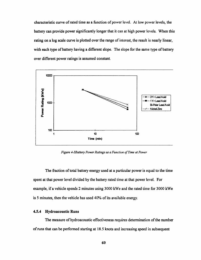
characteristic curve of rated time as a function of power level. At low power levels, the
battery can provide power significantly longer that it can at high power levels. When this
rating on a log scale curve is plotted over the range of interest, the result is nearly linear,
with each type of battery having a different slope. The slope for the same type of battery
over different power ratings is assumed constant.
10000
--- 3Yr Lead Acid5 -... 1 Yr LeadAcid
4 1Bi-Pda LeadAcid.... -- ..... Nid<ke-Zinm
1001 10 100
Time (min)
Figure 4-3Battery Power Ratings as a Function of Time at Power
The fraction of total battery energy used at a particular power is equal to the time
spent at that power level divided by the battery rated time at that power level. For
example, if a vehicle spends 2 minutes using 3000 kWe and the rated time for 3000 kWe
is 5 minutes, then the vehicle has used 40% of its available energy.
4.5.4 Hydroacoustic Runs
The measure of hydroacoustic effectiveness requires determination of the number
of runs that can be performed starting at 18.5 knots and increasing speed in subsequent

runs in increments in 5 knots. The final run may be performed at an increment of less
than 5 knots. Each attempt to obtain hydroacoustic data starts with submerging, pumping
out 90% of the trim tank water, and proceeding to the desired depth for the test. The
vehicle must remain at 8 knots until half of the trim tank has been pumped, after which
time speed is reduced to 4 knots. If the time submerged is less than 30 minutes, then the
vehicle must loiter at 4 knots to complete the instrumentation start-up procedure. [4,21]
The trim system pump for the LSV has a rated capacity of 30 gal/min. Assuming
the water is pumped out at a depth of 200 feet and the efficiency from the battery to water
pumped overboard is 70%, then 100 kW is required for the time that the pump is running.
The time the pump must run is 90% of the volume of the trim tank divided by the pump
capacity.
The power required to loiter at 4 and 8 knots is calculated from the powering
equation. The power used at the beginning of the run is the sum of the pump power and
propulsion power at 8 knots. The fraction of battery energy used is then calculated for
the time to pump half of the trim tank. The next step is to reduce speed to 4 knots and
pump the remainder of the trim tank. Again battery energy is calculated. The vehicle
then secures the pump and continues to loiter at 4 knots until the time submerged is
greater than 30 minutes. Battery energy is again calculated.
The vehicle is then ready to start its first run at 18.5 knots and travel through the
acoustic range. The time required to complete this evolution is approximately 3000 yards
divided by the vehicle speed. The actual distance on the range is somewhat less than
3000 yards, but the additional distance allows for acceleration. The power used by the
vehicle is calculated from the powering equation, taking into account PC and electrical to
mechanical efficiency. Using this power over the time to complete the run, the fraction
of battery energy used is calculated. If the total battery energy remains positive, then the
vehicle has successfully completed one run. If the calculated total battery energy
remaining is less than zero, then the vehicle does not have enough battery energy to
complete the run.
Before a second run can be started, the vehicle must loiter for 30 minutes at 4
knots to reposition for the next run and reset the instrumentation. The second run is
attempted at 23.5 knots (5 knots faster than the first run). Again the power and time
required for this run are calculated along with the fraction of battery energy used. If the
total battery energy remaining is positive, then another successful run is completed. If
not, the total battery energy is returned to energy available after the last loiter between
runs, and the speed is reduced from the previous unsuccessful run in 0.25 knot increments
until the maximum speed for hydroacoustic data collection is found. If the attempt at the
five-knot increase is successful, then the speed is again increased 5 knots (28.5 knots for
run 3) and the process is repeated until the maximum speed for hydroacoustic data
collection is found. A final check is made to ensure the maximum speed calculated for
hydroacoustic data collection does not exceed the vehicle maximum speed. If it does, the
maximum hydroacoustic speed is set to maximum vehicle speed.
4.5.5 Hydrodynamic Runs
The final MOP calculated is the number of data collection runs that can be
performed at Froude scale maximum speed. Assuming LSV is scaled to a submarine
with a 10,000 Lton submerged displacement, the scaling factor and Froude scale
maximum speed are:
Scale = fDisplacementbS10,0001ton
VFr = V (Scale)'2
The battery power required to propel the vehicle at this speed and the battery
energy for the time required to cover the 3000 yard course are then calculated. The total
number of Froude runs possible is the truncated result of battery energy available divided
by the energy required for each run.
4.6 Cost
The subroutine "Cost" calculates acquisition cost and discounted total ownership
cost for each LSV II option that is evaluated. All cost estimates are based on the LSV II
Al Total Ownership Cost Estimate [22] and are referenced to constant FY 98 dollars.
Dollars spent in future years are discounted at 6% per year.
4.6.1 Acquisition Cost
Acquisition cost is estimated by multiplying each weight group calculated by the
weight subroutine by a cost estimating relationship (CER) extracted from the cost
estimate for Al. The CERs are obtained by dividing the cost for each weight group by
the weight of that group in the estimate for Al. The weight groups that do not vary
between the variants are assigned a constant cost. Instrumentation is also assigned a
constant cost. Group 0, 8, and 9 are assigned a constant cost for design engineering, ship
support services, computer costs and travel.
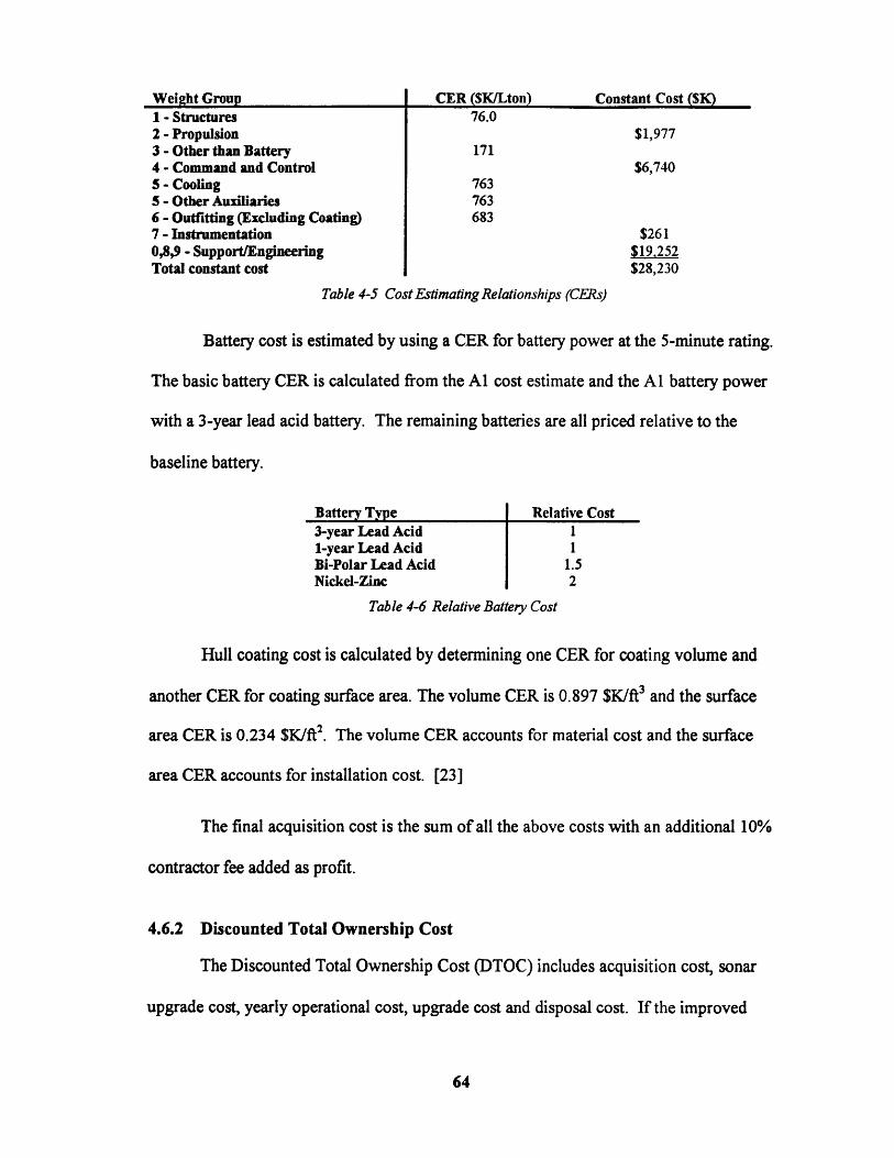
1 - Structures 76.02 - Propulsion $1,9773 - Other than Battery 1714 - Command and Control $6,7405 - Cooling 7635 - Other Auxiliaries 7636 - Outfitting (Excluding Coating) 6837 - Instrumentation $2610,8,9 -Support/Engineering $19,252Total constant cost $28,230
Table 4-5 Cost Estimating Relationships (CERs)
Battery cost is estimated by using a CER for battery power at the 5-minute rating.
The basic battery CER is calculated from the Al cost estimate and the Al battery power
with a 3-year lead acid battery. The remaining batteries are all priced relative to the
baseline battery.
Battery Type Relative Cost3-year Lead Acid 11-year Lead Acid 1Bi-Polar Lead Acid 1.5Nickel-Zinc 2
Table 4-6 Relative Battery Cost
Hull coating cost is calculated by determining one CER for coating volume and
another CER for coating surface area. The volume CER is 0.897 $K/ft3 and the surface
area CER is 0.234 $K/ft2 . The volume CER accounts for material cost and the surface
area CER accounts for installation cost. [23]
The final acquisition cost is the sum of all the above costs with an additional 10%
contractor fee added as profit.
4.6.2 Discounted Total Ownership Cost
The Discounted Total Ownership Cost (DTOC) includes acquisition cost, sonar
upgrade cost, yearly operational cost, upgrade cost and disposal cost. If the improved
CER ($K/Lton)Weight Group Constant Cost (SK)
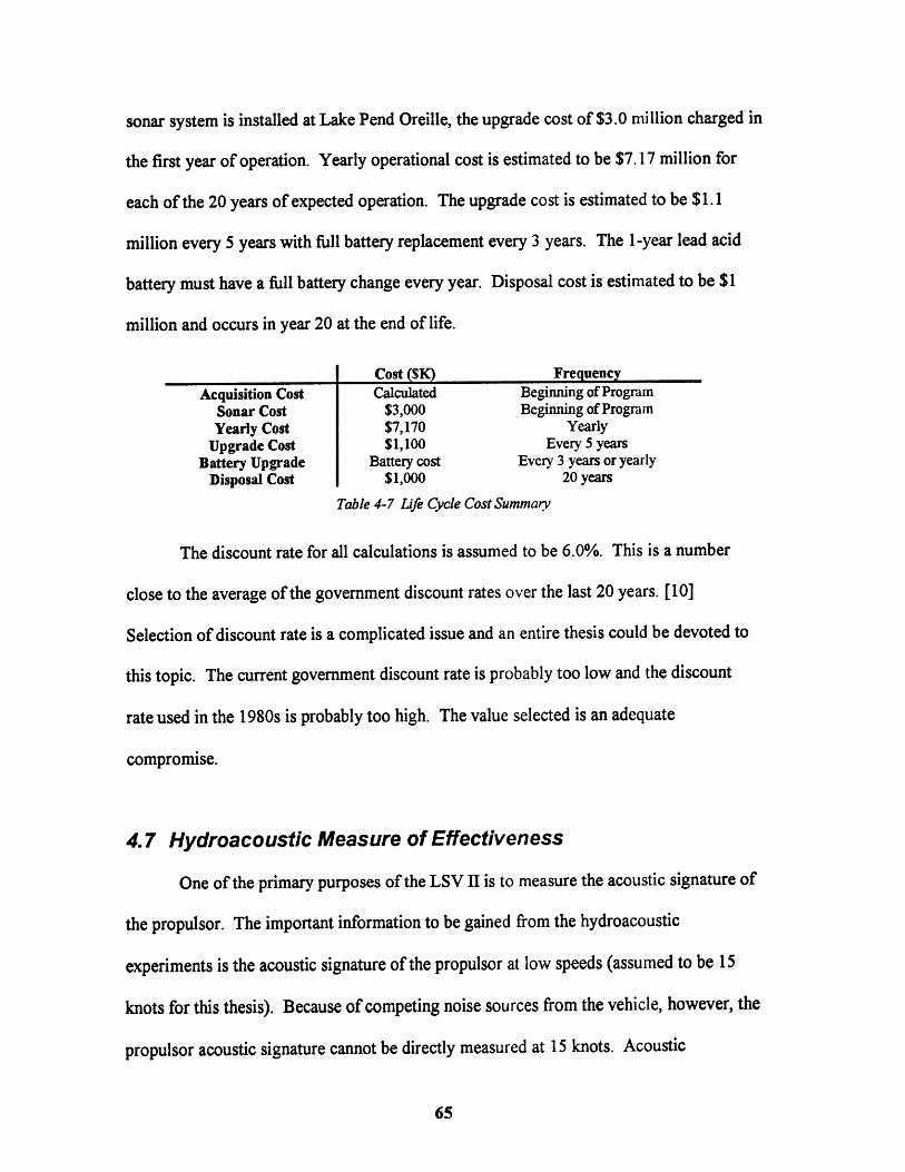
sonar system is installed at Lake Pend Oreille, the upgrade cost of $3.0 million charged in
the first year of operation. Yearly operational cost is estimated to be $7.17 million for
each of the 20 years of expected operation. The upgrade cost is estimated to be $1.1
million every 5 years with full battery replacement every 3 years. The 1-year lead acid
battery must have a full battery change every year. Disposal cost is estimated to be $1
million and occurs in year 20 at the end of life.
Cost (SK) FrequencyAcquisition Cost Calculated Beginning of Program
Sonar Cost $3,000 Beginning of ProgramYearly Cost $7,170 Yearly
Upgrade Cost $1,100 Every 5 yearsBattery Upgrade Battery cost Every 3 years or yearly
Disposal Cost $1,000 20 years
Table 4-7 Life Cycle Cost Summary
The discount rate for all calculations is assumed to be 6.0%. This is a number
close to the average of the government discount rates over the last 20 years. [10]
Selection of discount rate is a complicated issue and an entire thesis could be devoted to
this topic. The current government discount rate is probably too low and the discount
rate used in the 1980s is probably too high. The value selected is an adequate
compromise.
4.7 Hydroacoustic Measure of Effectiveness
One of the primary purposes of the LSV II is to measure the acoustic signature of
the propulsor. The important information to be gained from the hydroacoustic
experiments is the acoustic signature of the propulsor at low speeds (assumed to be 15
knots for this thesis). Because of competing noise sources from the vehicle, however, the
propulsor acoustic signature cannot be directly measured at 15 knots. Acoustic
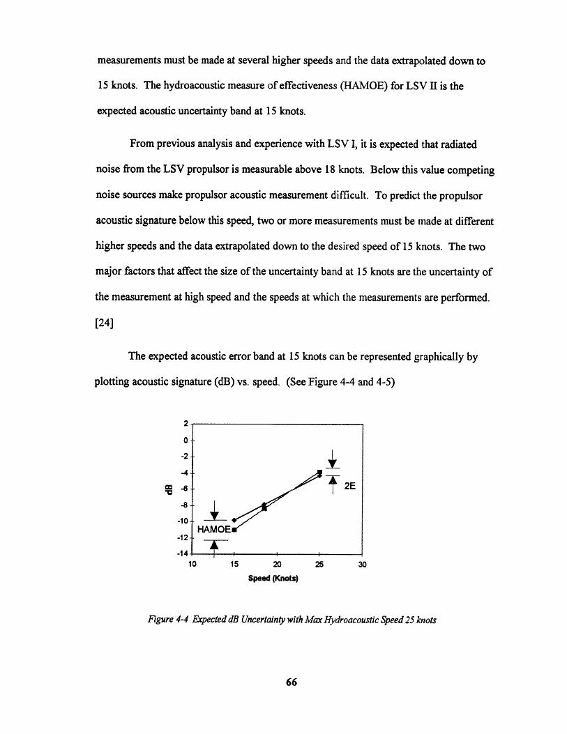
measurements must be made at several higher speeds and the data extrapolated down to
15 knots. The hydroacoustic measure of effectiveness (HAMOE) for LSV II is the
expected acoustic uncertainty band at 15 knots.
From previous analysis and experience with LSV I, it is expected that radiated
noise from the LSV propulsor is measurable above 18 knots. Below this value competing
noise sources make propulsor acoustic measurement difficult. To predict the propulsor
acoustic signature below this speed, two or more measurements must be made at different
higher speeds and the data extrapolated down to the desired speed of 15 knots. The two
major factors that affect the size of the uncertainty band at 15 knots are the uncertainty of
the measurement at high speed and the speeds at which the measurements are performed.
[24]
The expected acoustic error band at 15 knots can be represented graphically by
plotting acoustic signature (dB) vs. speed. (See Figure 4-4 and 4-5)
2
0
-26 2E-4
HAMOE-12
-14 4-10 15 20 25 30
Speed (Knots)
Figure 4-4 Expected dB Uncertainty with Max Hydroacoustic Speed 25 knots
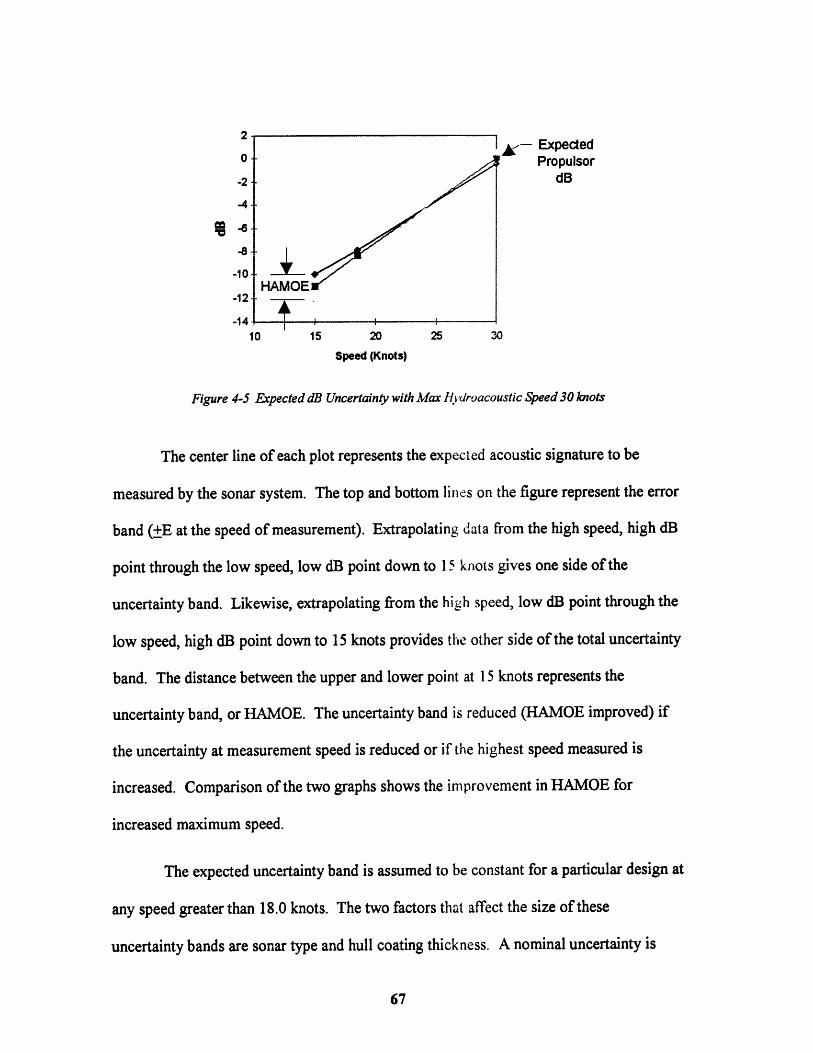
0 A- Expected,0 Propulsor
-2 dB
-4
-10
HAMOE-12
10 15 20 25 30
Speed (Knots)
Figure 4-5 Expected dB Uncertainty with Max Hydroacoustic Speed 30 knots
The center line of each plot represents the expected acoustic signature to be
measured by the sonar system. The top and bottom lines on the figure represent the error
band (+E at the speed of measurement). Extrapolating data from the high speed, high dB
point through the low speed, low dB point down to 15 knots gives one side of the
uncertainty band. Likewise, extrapolating from the high speed, low dB point through the
low speed, high dB point down to 15 knots provides the other side of the total uncertainty
band. The distance between the upper and lower point at 15 knots represents the
uncertainty band, or HAMOE. The uncertainty band is reduced (HAMOE improved) if
the uncertainty at measurement speed is reduced or if the highest speed measured is
increased. Comparison of the two graphs shows the improvement in HAMOE for
increased maximum speed.
The expected uncertainty band is assumed to be constant for a particular design at
any speed greater than 18.0 knots. The two factors that affect the size of these
uncertainty bands are sonar type and hull coating thickness. A nominal uncertainty is
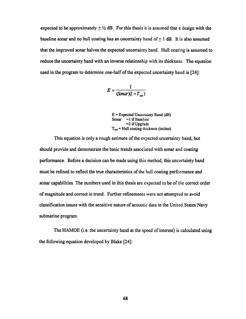
expected to be approximately + /2 dB. For this thesis it is assumed that a design with the
baseline sonar and no hull coating has an uncertainty band of + 1 dB. It is also assumed
that the improved sonar halves the expected uncertainty band. Hull coating is assumed to
reduce the uncertainty band with an inverse relationship with its thickness. The equation
used in the program to determine one-half of the expected uncertainty band is [24]:
1(Sonar)(1 +, )
E = Expected Uncertainty Band (dB)Sonar =1 if Baseline
=2 if UpgradeTc = Hull coating thickness (inches)
This equation is only a rough estimate of the expected uncertainty band, but
should provide and demonstrate the basic trends associated with sonar and coating
performance. Before a decision can be made using this method, this uncertainty band
must be refined to reflect the true characteristics of the hull coating performance and
sonar capabilities. The numbers used in this thesis are expected to be of the correct order
of magnitude and correct in trend. Further refinements were not attempted to avoid
classification issues with the sensitive nature of acoustic data in the United States Navy
submarine program.
The HAMOE (i.e. the uncertainty band at the speed of interest) is calculated using
the following equation developed by Blake [24]:
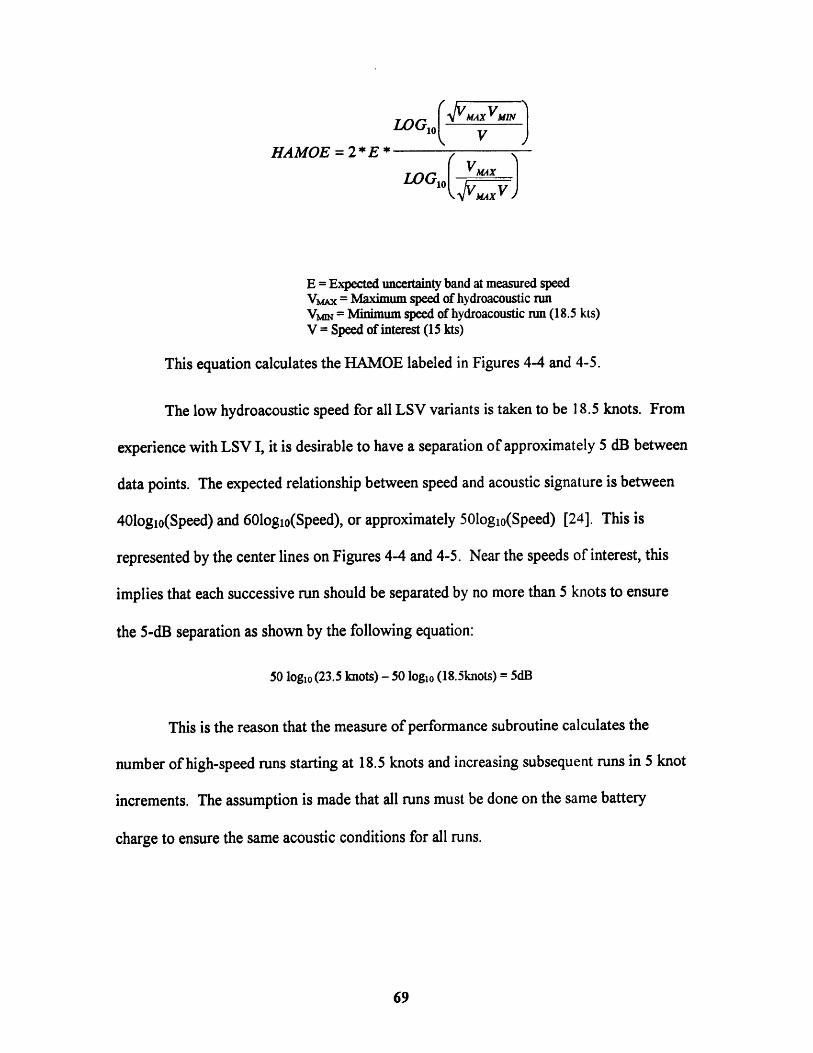
LOGII MAXVMhJ
HAMOE = 2 * E *
LOGIO ,V-x
E = Expected uncertainty band at measured speedVmAx = Maximum speed of hydroacoustic runVMm = Minimum speed of hydroacoustic run (18.5 kts)V = Speed of interest (15 kts)
This equation calculates the HAMOE labeled in Figures 4-4 and 4-5.
The low hydroacoustic speed for all LSV variants is taken to be 18.5 knots. From
experience with LSV I, it is desirable to have a separation of approximately 5 dB between
data points. The expected relationship between speed and acoustic signature is between
40logio(Speed) and 60loglo(Speed), or approximately 50loglo(Speed) [24]. This is
represented by the center lines on Figures 4-4 and 4-5. Near the speeds of interest, this
implies that each successive run should be separated by no more than 5 knots to ensure
the 5-dB separation as shown by the following equation:
50 logo (23.5 knots) - 50 logo (18.5knots) = 5dB
This is the reason that the measure of performance subroutine calculates the
number of high-speed runs starting at 18.5 knots and increasing subsequent runs in 5 knot
increments. The assumption is made that all runs must be done on the same battery
charge to ensure the same acoustic conditions for all runs.
4.8 Hydrodynamic and Flexibility Combined Measure of
Effectiveness
The hydroacoustic and flexibility attribute involves more than one performance
metric. Expert opinion is used to establish and synthesize the relative value of 3
measures of performance into a CMOE: Number of Runs at Froude Scale Maximum
Speed, Margin and Geo-similitude. Two methods of collecting this expert opinion are
investigated: Multi-Attribute Iso-effectiveness (MAIE) and Analytical Hierarchy
Process (AHP). MAIE is used in the computer model to synthesize the CMOE and AHP
is used for comparison purposes. Appendix A contains the survey results from the two
methods.
Both methods require the determination of goals and thresholds for each variable.
The following goals and thresholds are used:
Number of Runs at Froude Scale Speed that can be performed on one battery charge.Goal = 10, Threshold = 7
Amount of margin that is available for future growth, including propulsor installation.Goal = 12%, Threshold = 3% (Variant Al currently has a value of 6.3%)
The type of geo-similitude that is chosen.Options: NSSN, SSN-21, None (i.e. has "submarine-like shape")
Goals represent the best value the decision maker believes to be obtainable with
the technology available in the time frame of the project, or the value at which further
improvement no longer adds significant improvement to the project. Thresholds
represent the value of worst acceptable performance. Below this value, it is considered
not worth continuing with the project.
If a variant achieves values above the goal, no additional credit is given. It is
treated the same as if it had only achieved the goal. If any value is below the threshold,
the LSV is assumed to be not feasible. Selection of appropriate variables and goals and
thresholds is extremely important, because if this first step of the process is flawed, the
remainder of the process does not give meaningful results.
The AHP method requires the expert to make a set of pair-wise comparisons
using a questionnaire. First the relative importance of each of the variables is compared.
Specifically, the expert must compare Geo-similitude to Margin, Geo-similitude to
Number of Froude Scale Runs (FSRs), and Margin to Number of Froude Scale Runs.
Each of the specific values under each category is then compared to each other specific
value within its category. All comparisons are on a scale from 1 to 9, with 1 indicating
the choices are equal and 9 indicating that one option is extremely more important than
the other. The data is then analyzed using "Expert Choice" software in the distributive
mode. Appendix A contains the AHP survey and results. [15]
The input required for the Multi-Attribute Iso-effectiveness is obtained by having
the expert answer a set of questions to generate a set of iso-effectiveness curves. An iso-
effectiveness curve represents the combination of characteristics with which the decision-
maker is equally satisfied. For example, if one of the variables is held constant, how
much change is required in each of the two remaining variables to give equal
effectiveness? Specifically, if geo-similitude is held constant, what value of margin
combined with 9 Froude Scale Runs gives equal effectiveness to 10 Froude Scale Runs
and 3% margin? This question is occasionally difficult for experts to answer initially, so
the expert is encouraged to bracket the answer until the equivalence point is reached. For
example, 12% margin is probably preferred, but 3.5% is probably not. Appendix A gives
the complete survey along with a plot of iso-effectiveness lines.
The information from the iso-effectiveness curves is entered into the subroutine
"Calc HAMOE." The output of HAMOE is an "equivalent margin." If the geo-
similitude is "none" and the Number of Froude Scale Runs is the threshold value (7), then
the equivalent margin is the vehicle margin. If however, geo-similitude or FSRs is
greater than the threshold, then the equivalent margin is increased to the point that the
decision maker is equally satisfied with the variant's attributes and one with the
equivalent margin, no geo-similitude and threshold FSRs.
To graphically see the process of equivalent margin, assume the LSV variant
under consideration has an SSN-21 geo-similitude, 8% margin and is capable of 8 FSRs.
Entering the Iso-Effectiveness with Froude Run Constant graph (Figure 4-6) at SSN-21,
8% yields a point between the top two iso-effectiveness lines. Interpolating between the
two lines at the no geo-similitude location to the same linear proportion as at the SSN-21
geo-similitude yields an intermediate equivalent margin of 9%. If the FSRs were at the
threshold value, this would be the final equivalent margin.
Since FSRs equals 8, the Iso-Effectiveness with Geo-similitude constant graph
(Figure 4-7) must be entered at 8 FSRs and the intermediate equivalent margin of 9%,
which yields a point between the top two iso-effectiveness lines on this graph.
Interpolating between the two lines at the FSRs equal 7 location yields the final
equivalent margin of 9.5%. This is the final value for the hydrodynamic and flexibility
measure of effectiveness.
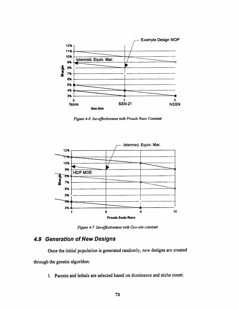
- Example Design MOP12%11%: -
10%.Intermed. Equiv. Mar.
8% -
7%
6%
5%
4%
3%10 1
None SSN-21Geo-Sim
Figure 4-6 Iso-effectiveness with Froude Runs Constant
2NSSN
Intermed. Equiv. Mar.
7 8 9 10
Froude Scale Runs
Figure 4-7 Iso-effectiveness with Geo-sim constant
4.9 Generation of New Designs
Once the initial population is generated randomly, new designs are created
through the genetic algorithm:
1. Parents and lethals are selected based on dominance and niche count.
"" ~"""*-- -- -- ~.~,~,__~~_
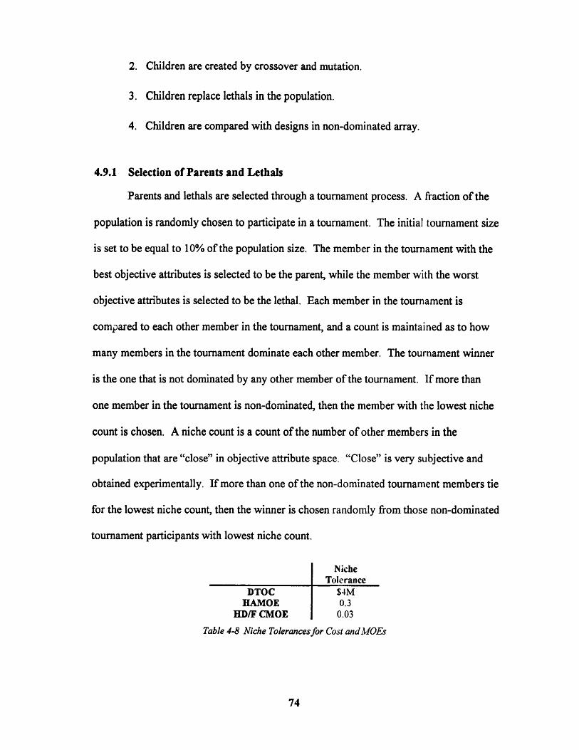
2. Children are created by crossover and mutation.
3. Children replace lethals in the population.
4. Children are compared with designs in non-dominated array.
4.9.1 Selection of Parents and Lethals
Parents and lethals are selected through a tournament process. A fraction of the
population is randomly chosen to participate in a tournament. The initial tournament size
is set to be equal to 10% of the population size. The member in the tournament with the
best objective attributes is selected to be the parent, while the member with the worst
objective attributes is selected to be the lethal. Each member in the tournament is
compared to each other member in the tournament, and a count is maintained as to how
many members in the tournament dominate each other member. The tournament winner
is the one that is not dominated by any other member of the tournament. If more than
one member in the tournament is non-dominated, then the member with the lowest niche
count is chosen. A niche count is a count of the number of other members in the
population that are "close" in objective attribute space. "Close" is very subjective and
obtained experimentally. If more than one of the non-dominated tournament members tie
for the lowest niche count, then the winner is chosen randomly from those non-dominated
tournament participants with lowest niche count.
NicheTolerance
DTOC $4MHAMOE 0.3
HD/F CMOE 0.03
Table 4-8 Niche Tolerances for Cost andMOEs
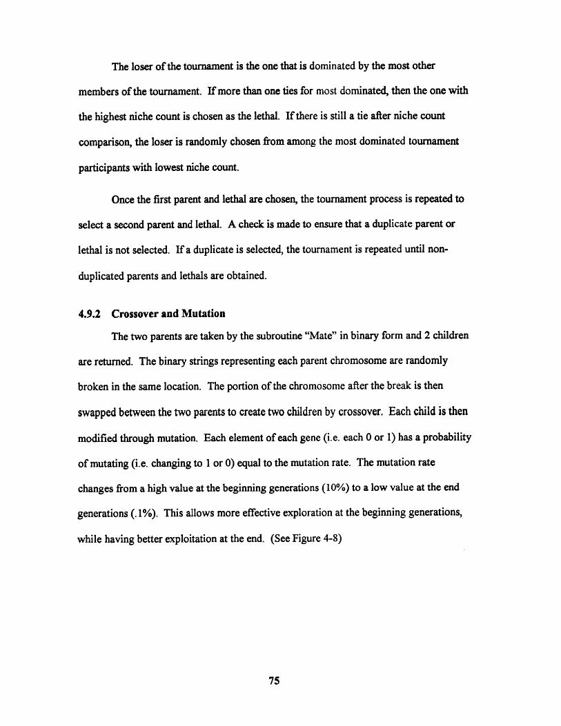
The loser of the tournament is the one that is dominated by the most other
members of the tournament. If more than one ties for most dominated, then the one with
the highest niche count is chosen as the lethal. If there is still a tie after niche count
comparison, the loser is randomly chosen from among the most dominated tournament
participants with lowest niche count.
Once the first parent and lethal are chosen, the tournament process is repeated to
select a second parent and lethal. A check is made to ensure that a duplicate parent or
lethal is not selected. If a duplicate is selected, the tournament is repeated until non-
duplicated parents and lethals are obtained.
4.9.2 Crossover and Mutation
The two parents are taken by the subroutine "Mate" in binary form and 2 children
are returned. The binary strings representing each parent chromosome are randomly
broken in the same location. The portion of the chromosome after the break is then
swapped between the two parents to create two children by crossover. Each child is then
modified through mutation. Each element of each gene (i.e. each 0 or 1) has a probability
of mutating (i.e. changing to 1 or 0) equal to the mutation rate. The mutation rate
changes from a high value at the beginning generations (10%) to a low value at the end
generations (. 1%). This allows more effective exploration at the beginning generations,
while having better exploitation at the end. (See Figure 4-8)
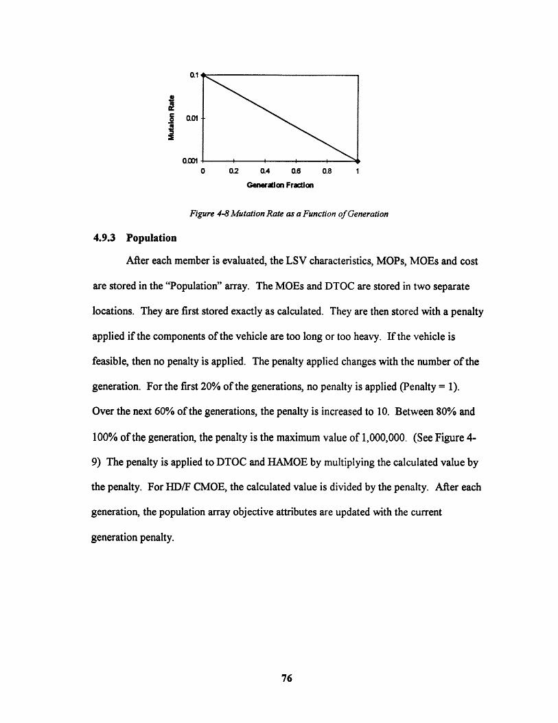
'U I
0 0.2 0.4 0.6 0.8 1
Generation Fraction
Figure 4-8 Mutation Rate as a Function of Generation
4.9.3 Population
After each member is evaluated, the LSV characteristics, MOPs, MOEs and cost
are stored in the "Population" array. The MOEs and DTOC are stored in two separate
locations. They are first stored exactly as calculated. They are then stored with a penalty
applied if the components of the vehicle are too long or too heavy. If the vehicle is
feasible, then no penalty is applied. The penalty applied changes with the number of the
generation. For the first 20% of the generations, no penalty is applied (Penalty = 1).
Over the next 60% of the generations, the penalty is increased to 10. Between 80% and
100% of the generation, the penalty is the maximum value of 1,000,000. (See Figure 4-
9) The penalty is applied to DTOC and HAMOE by multiplying the calculated value by
the penalty. For HD/F CMOE, the calculated value is divided by the penalty. After each
generation, the population array objective attributes are updated with the current
generation penalty.
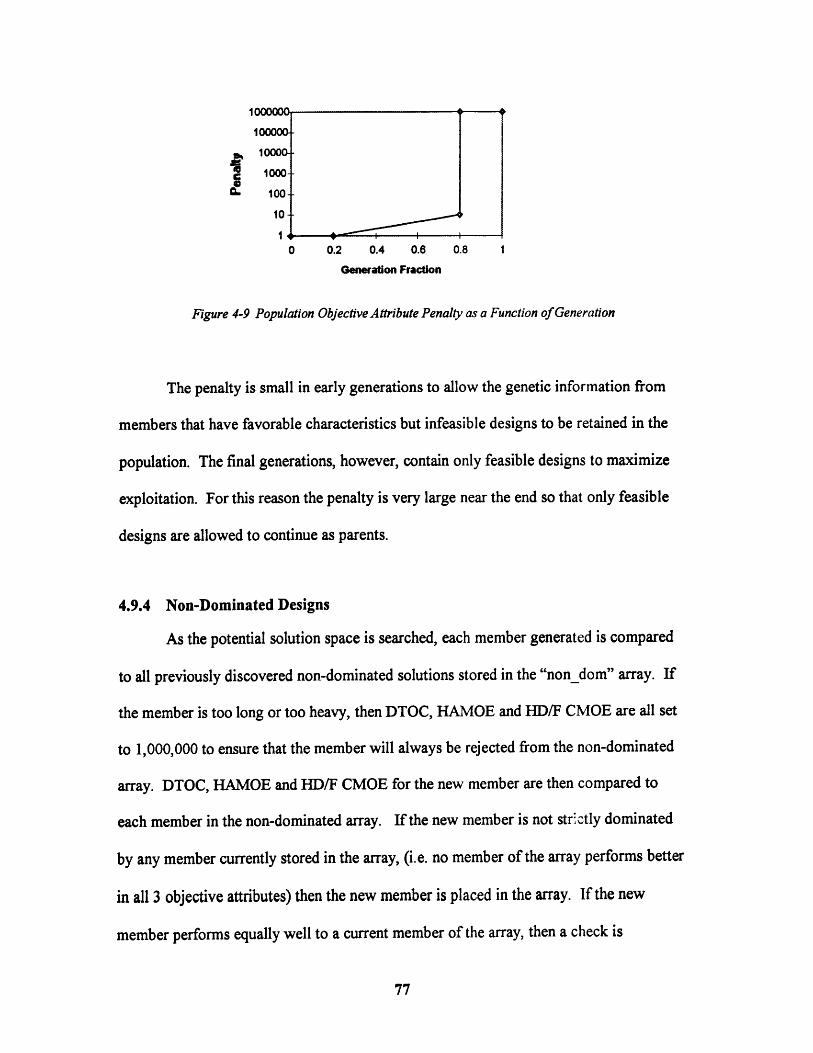
1000000
S10000-
i 10000
ioooco
10
0 0.2 0.4 0.6 0.8 1
Generation Fraction
Figure 4-9 Population Objective Attribute Penalty as a Function of Generation
The penalty is small in early generations to allow the genetic information from
members that have favorable characteristics but infeasible designs to be retained in the
population. The final generations, however, contain only feasible designs to maximize
exploitation. For this reason the penalty is very large near the end so that only feasible
designs are allowed to continue as parents.
4.9.4 Non-Dominated Designs
As the potential solution space is searched, each member generated is compared
to all previously discovered non-dominated solutions stored in the "non_dom" array. If
the member is too long or too heavy, then DTOC, HAMOE and HD/F CMOE are all set
to 1,000,000 to ensure that the member will always be rejected from the non-dominated
array. DTOC, HAMOE and HD/F CMOE for the new member are then compared to
each member in the non-dominated array. If the new member is not strictly dominated
by any member currently stored in the array, (i.e. no member of the array performs better
in all 3 objective attributes) then the new member is placed in the array. If the new
member performs equally well to a current member of the array, then a check is
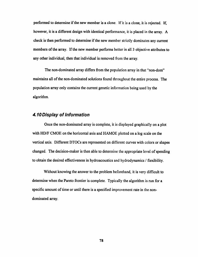
performed to determine if the new member is a clone. If it is a clone, it is rejected. If,
however, it is a different design with identical performance, it is placed in the array. A
check is then performed to determine if the new member strictly dominates any current
members of the array. If the new member performs better in all 3 objective attributes to
any other individual, then that individual is removed from the array.
The non-dominated array differs from the population array in that "non-dom"
maintains all of the non-dominated solutions found throughout the entire process. The
population array only contains the current genetic information being used by the
algorithm.
4.10 Display of Information
Once the non-dominated array is complete, it is displayed graphically on a plot
with HD/F CMOE on the horizontal axis and HAMOE plotted on a log scale on the
vertical axis. Different DTOCs are represented on different curves with colors or shapes
changed. The decision-maker is then able to determine the appropriate level of spending
to obtain the desired effectiveness in hydroacoustics and hydrodynamics / flexibility.
Without knowing the answer to the problem beforehand, it is very difficult to
determine when the Pareto frontier is complete. Typically the algorithm is run for a
specific amount of time or until there is a specified improvement rate in the non-
dominated array.
5Tuning the Genetic Algorithm
Once the evolutionary program has been developed, the parameters of the genetic
algorithm must be adjusted to optimize search performance. The design evaluator for
LSV II is fast enough that an exhaustive search of all possible designs can be performed
and used to tune the genetic algorithm. This thesis refers to the complete process as the
evolutionary program and the specific parts dealing with selection and mating as the
genetic algorithm.
5.1 Exhaustive Search
Initial data runs of the evolutionary program indicated that the entire space could
be searched in a reasonable amount of time. An exhaustive search is often not feasible in
design problems because of the amount of time required to perform an evaluation of the
large number of possible design alternatives. An evaluation of each LSV design requires
approximately 0.01 seconds on a 133 MHz Intel Pentium Processor using 16 MB of
RAM. The initial design parameter space includes 4.2 million possible combinations, so
the entire space can be searched in just over 12 hours.
An exhaustive search was performed to determine the Pareto frontier for the
initial design space. The exhaustive search data was used to fine-tune the genetic
algorithm. The complete set of non-dominated designs was compared to the non-
dominated designs found using the evolutionary program to obtain a metric for
performance of the evolutionary program. The exhaustive search data was also used to
analyze trends in objective attribute space and evaluation of design parameter limits.
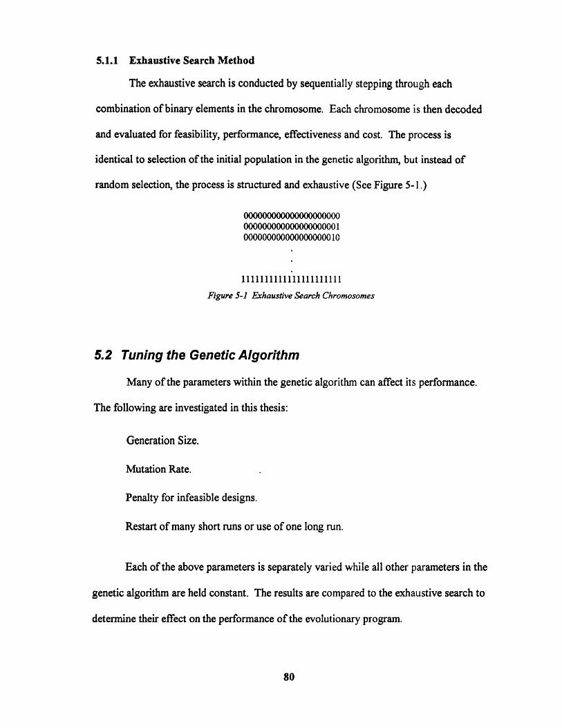
5.1.1 Exhaustive Search Method
The exhaustive search is conducted by sequentially stepping through each
combination of binary elements in the chromosome. Each chromosome is then decoded
and evaluated for feasibility, performance, effectiveness and cost. The process is
identical to selection of the initial population in the genetic algorithm, but instead of
random selection, the process is structured and exhaustive (See Figure 5-1.)
00000000000000000000o00000000000000000001000000000000000000010
1111111111111111111111
Figure 5-1 Exhaustive Search Chromosomes
5.2 Tuning the Genetic Algorithm
Many of the parameters within the genetic algorithm can affect its performance.
The following are investigated in this thesis:
Generation Size.
Mutation Rate.
Penalty for infeasible designs.
Restart of many short runs or use of one long run.
Each of the above parameters is separately varied while all other parameters in the
genetic algorithm are held constant. The results are compared to the exhaustive search to
determine their effect on the performance of the evolutionary program.

5.2.1 Generation Size
Generation sizes of 150, 200, 250, 300 and 350 are compared in an attempt to
determine the optimum generation size. The generation size sets the initial number of
members in the population. A new generation is finished when the number of children
created in that generation equals the generation size. Increasing the generation size
introduces more genetic information into the algorithm, but also requires more computer
time per design evaluation. Time to complete each evaluation is an exponential function
of the generation size. (See Figure 5-2)
0.16
0.14
0.12
0.1
0.08
0.06
0.04
0.02
0 I
0 50 100 150 200 250 300 350
Generation Size
Figure 5-2 Average Time per Evaluation as a Function of Generation Size
In this particular problem, the time to evaluate each design is on the same order of
magnitude as the time to perform the genetic algorithm. The difference between the 0.03
seconds required for a generation size of 150 and the 0.16 seconds for a generation size

of 350 is significant. In the case of a more complicated problem, where the time to
evaluate each design requires several orders of magnitude more time than the genetic
algorithm, however, this time difference is insignificant. Because this thesis is
attempting to show the possible effects of this method on full scale ship design, the time
required for genetic algorithm processing is ignored. For this reason, all comparisons are
made with number of evaluations required rather than amount of time to required to
execute the program.
Figures 5-3 and 5-4 indicate that in general, more non-dominated designs are
found more quickly with a larger generation size. The line labeled as random shows the
expected rate of finding non-dominated designs using a random search of the design
space. The smaller the slope of these curves the better the performance of the search.
When compared with the random search, all of the evolutionary programs perform well
no matter which parameters are used.
Figure 5-3 shows only the evolutionary program results. It can be seen that early
in the process there is little difference in the performance of different generation sizes,
and in several places, the curves actually cross. At the end of the plot, however, the
larger generation sizes perform better.

-a
S600000 - Generation
m Size5 000 -0_ Randon
40000W - ---- 150
----- 2500 200000 -
Z - 350
10000- -
0 10 20 30 40 50 60
Number of Non-dominated Designs Found
Figure 5-3 Program Performance with Varying Generation Size Compared to Random Search
140000
A 120000
Generation100000 /o
._ Size
O 80000 -
-150.'.. -- 250
Z20000 .
0 10 20 30 40 50 60
Number of Non-dominated Designs Found
Figure 5-4 Program Performance with Varying Generation Size
5.2.2 Mutation Rate
Mutation rate is varied between 0.1 and 0.001. The first run uses a mutation rate
that starts at 0.1 for the initial generations and ends at 0.001 for the final generations.
The second run starts at 0.1 and ends at 0.01. The other three runs all use constant
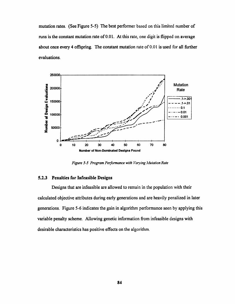
mutation rates. (See Figure 5-5) The best performer based on this limited number of
runs is the constant mutation rate of 0.01. At this rate, one digit is flipped on average
about once every 4 offspring. The constant mutation rate of 0.01 is used for all further
evaluations.
C1 2
wiC
CM
EZ
MutationRate
0 10 20 30 40 50 60 70 80
Number of Non-Dominated Designs Found
Figure 5-5 Program Performance with Varying Mutation Rate
5.2.3 Penalties for Infeasible Designs
Designs that are infeasible are allowed to remain in the population with their
calculated objective attributes during early generations and are heavily penalized in later
generations. Figure 5-6 indicates the gain in algorithm performance seen by applying this
variable penalty scheme. Allowing genetic information from infeasible designs with
desirable characteristics has positive effects on the algorithm.
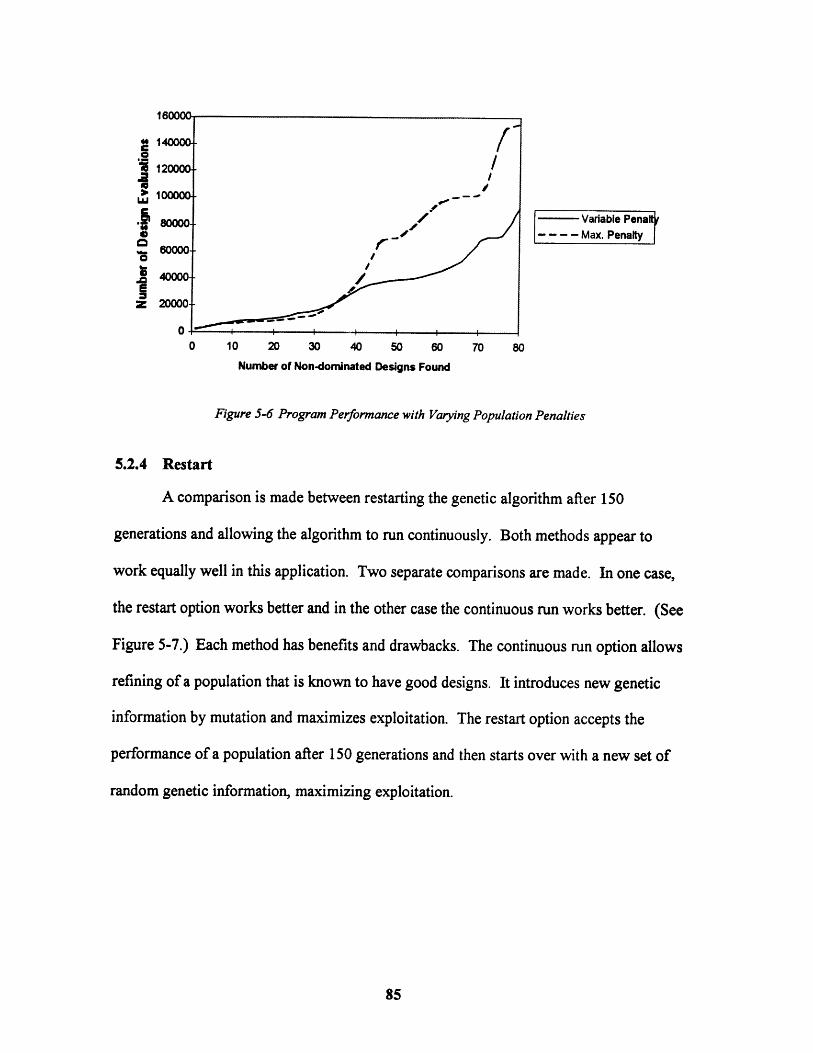
C1 /
120000-
1000001 ---
S80000 / - Variable Penalt-- - - -Max. Penalty
60000.01
0 10 20 30 40 50 60 70 80
Number of Non-dominated Designs Found
Figure 5-6 Program Performance with Varying Population Penalties
5.2.4 Restart
A comparison is made between restarting the genetic algorithm after 150
generations and allowing the algorithm to run continuously. Both methods appear to
work equally well in this application. Two separate comparisons are made. In one case,
the restart option works better and in the other case the continuous run works better. (See
Figure 5-7.) Each method has benefits and drawbacks. The continuous run option allows
refining of a population that is known to have good designs. It introduces new genetic
information by mutation and maximizes exploitation. The restart option accepts the
performance of a population after 150 generations and then starts over with a new set of
random genetic information, maximizing exploitation.

S100000 ./
Run Number80000-
/ Generation SizeS60M-
/ /
- --- 2-5X50 Ge.40000-*40.00- ....... 1-750 Gen.--. - 2- 5X150 Ger.
20000- -" -
0-0 10 20 30 40 50 60 70
Number of Non-Dominated Designs Found
Figure 5-7 Program Performance Comparing Restart vs. Large number ofgenerations
5.3 Conclusion
The analysis of varying the parameters of the genetic algorithm indicates the
evolutionary program is very robust and works well over a wide range of parameters.

6Results
Chapter 6 discusses the specific results obtained from the evolutionary program
applied to the design of Large Scale Vehicle II.
6.1 Objective Attribute Trends on the Pareto Frontier
An analysis of the Pareto frontier generated from the exhaustive search is
discussed in this section. Figure 6-1 is a plot of the Pareto frontier for selected costs.
Appendix B contains the complete plot and the characteristics of each design found by
exhaustive search. The non-dominated designs tend to congregate in 5 different regions.
The regions are represented by ovals on the Pareto frontier plot of the exhaustive search.
6.1.1 Pareto Frontier Plot Explanation
The vertical axis of Figure 6-1 represents the hydroacoustic measure of
effectiveness (HAMOE). It is plotted on a logarithmic scale because it represents an
acoustic uncertainty band that is measured in decibels. The horizontal axis represents
hydrodynamic and flexibility combined of effectiveness (HD/F CMOE), which is based
on an expert opinion combination of geo-similitude, number of Froude scale maximum
speed runs (FSRs) and margin. The base score for HD/F CMOE is the design's margin,
and additional credit is given by the MAIE method for improvements above the threshold
in geo-similitude and number of FSRs. It is plotted on a linear scale because it is closely
related to margin, which is represented well with a linear display. The negative value of
HD/F CMOE is plotted so that all objective attributes are better as low values. In this
way the algorithm attempts to minimize all 3 objective attributes rather than minimizing
some while maximizing others.
Each different symbol represents a different discounted total ownership cost
(DTOC) in millions of dollars. On Figure 6-1, all designs with a common DTOC are
connected with a constant cost line. Each design that was found by the exhaustive search
to be non-dominated is represented by a symbol on the plot. The type of symbol
represents its DTOC and its location on the plot represents its HAMOE and HD/F
CMOE. The least effective and least expensive variants are located in the upper right
hand corner of the plot, and the most effective and most expensive variants are located in
the lower left hand corner of the plot.
6.1.2 Pareto Frontier: Exhaustive Search
This section explains the reasons for the groupings on the Pareto frontier found by
exhaustive search. The numbered regions in the following discussion refer to the oval
regions on Figure 6-1.

Figure 6-1 Pareto Frontier: Exhaustive Search
10
0.1 --0.18 -0.16 -0.14 -0.12 -0.1 -0.08 -0.06
-(Hydrodynamic and Flexibility CMOE)
All designs on Figure 6-1 exceed the goal in number of Froude scale runs and
therefore receive the maximum increase in HD/F CMOE allowed for number of FSRs.
This is because all variants that perform well enough to attain a reasonable HAMOE also
perform well in number of FSRs due to their better endurance at higher speeds. At the
margin goal of 12%, the increase in score is 0.03. Therefore, a design with margin and
FSRs at the goal values attains a HD/F CMOE of 0.15 without geo-similitude of New
Attack or Seawolf. (Extreme left side of Regions 4 and 5.) The only way to achieve a
better score than 0.15 is with geo-similitude. (Regions 1 and 2.)
Regions 1 and 2 are areas of increased hydrodynamic performance due to geo-
similitude (geo-sim). Region 1 contains all of the New Attack geo-sim variants and
Region 2 contains most of the Seawolf variants. Since New Attack is the preferred geo-
sim, it attains the highest scores for HD/F CMOE (an increase of 0.02 with margin and
FSRs at the goal) . The New Attack is "long and thin", but has relatively high resistance,
which leads to poor performance in maximum speed and endurance. There is no New
Attack geo-sim on the Pareto frontier below the HD/F CMOE score 0.17. The Seawolf
geo-sim has better resistance characteristics than the New Attack, but not as good as
many of the other variants in the design space. The maximum HD/F CMOE for a
Seawolf variant is 0.16. Between 0.15 and 0.16 are only Seawolf variants.
Region 3 contains the least expensive variants. All of the designs in this region
have minimal hull coating and the baseline sonar system. This is the least expensive
method to build the LSV II, and hence produces the designs with the worst effectiveness.
Region 4 contains the designs with moderate effectiveness. All of the variants
within this region have either maximum hull coating and the baseline sonar system, or
minimal coating and the upgraded sonar system. The compromise on design parameters
yields the middle of the road effectiveness and relatively low cost.
Region 5 contains the majority of the non-dominated designs. All of the designs
in this region have the maximum hull coating and upgraded sonar system. This region of
the Pareto frontier is very nearly flat because the hull coating thickness is at its maximum
allowed value. The only way to improve HAMOE is to increase the vehicle maximum
speed, but at the high speeds, the powering curve is very steep. To increase vehicle speed
by even a small fraction requires a large amount of margin to be sacrificed for additional
batteries.
The design with the best effectiveness and highest cost in the design space is
plotted in the lower left hand corner. It is a New Attack geo-sim with upgraded sonar
system and maximum coating. It has high maximum speed at 36.9 knots due to its
advanced battery (Nickel-Zinc) and high battery power. It has the highest battery power
rating at 5100 kWe of any non-dominated design. It also has the highest acquisition cost
at $59.2 million.
6.1.3 Margin as a Measure of Effectiveness
There are very few gradual changes in the Pareto frontier, primarily because of
the goals and thresholds selected for measures of performance, the limits placed on
design parameter space and the method used to determine HD/F CMOE. To illustrate
this point, the exhaustive search was repeated, but instead of using the expert opinion
HD/F CMOE, only margin was used as the measures of effectiveness. A representative

sample of the Pareto frontier with margin is presented in Figure 6-2. Many of the sets of
DTOC points were eliminated for ease of presentation.
Most of the cost curves to the left of the margin goal of 12% have a knee before
they approach the margin goal. The left end of each curve (poor HAMOE and best
margin) represents slow vehicles that have minimal coating and the baseline sonar
system. The steep part of the curve is created because a small increase in coating
provides a relatively large improvement in HAMOE. At a certain point, it becomes more
cost effective to upgrade the sonar system instead of increasing coating thickness. At that
point, a shift is made from maximum coating thickness to minimal coating thickness with
upgraded sonar system. Improvement in HAMOE then comes from increases in coating
thickness. As coating thickness increases, speed of the vehicle drops off because of
increased resistance. When the maximum thickness allowed is reached the only method
available to improve HAMOE is to increase the vehicle maximum speed by lowering
resistance or increasing power. Reducing the hull size decreases resistance; increasing
battery size increases power. Both methods require sacrificing large amounts of margin,
which causes the shallow part of the curve.
Another interesting point about the margin Pareto frontier is there are no Seawolf
or New Attack variants on this frontier. All Seawolf and New Attack variants are
dominated. Since all variants found by the exhaustive search have goal performance in
FSRs, it is clear that the only reason variants with geo-similitude are on the frontier for
HD/F CMOE is because of the added value directly attributed to geo-similitude.

Figure 6-2 Partial Pareto Frontier: Exhaustive Searchwl Margin as MOE
10
+ oo DTOC
x ($M)
+ e139
SX X 0140
XX XXXA 141EXE
X 142
rs0 x 144
0 Knees 0149
+ aA0 +153
on l -157SU
- 161** fl 0 0 *167
0173
-L 0O A 1794- W X X x 187
-- + ,o 0 +
Higher Cost/Better Effectiveness Margin Goal (12%)
0.1 I-0.3 -0.25 -0.2 -0.15 -0.1 -0.05
-(Margin)
6.2 Comparison of Evolutionary Program Search
to Exhaustive Search
This section evaluates the effectiveness of an evolutionary program search by
comparison to the exhaustive search results. Evolutionary program results using a 200-
member population and 40 generations (8,000 evaluations) are presented in Figure 6-3.
The results from this same population extended through 80, 120 and 160 generations are
presented in Figures 6-4, 6-5 and 6-6 respectively.
After 8,000 evaluations of the 4.2 million possible designs (Figure 6-3) the basic
shape of the Pareto frontier can be seen in the 147 potentially non-dominated designs
found.3 When compared to the exhaustive search results, the range of DTOC and MOEs
is very closely predicted, although only 18 of the 295 absolutely non-dominated designs
have been found. 4 (See Table 6-1 for non-dominated design totals.) Regions 1 and 5
from the exhaustive search are very closely approximated. Although not all of the points
are present, the trend of the curves in these two regions is nearly identical to the
exhaustive search. Region 3 from the exhaustive search contains only designs with a
DTOC of $139M. Two of these designs were found with the evolutionary program, and
the remainder of the $140M points approximates the rest of region 3 fairly well. Region
4 has very few points and no trend can be obtained from the data. Region 2 has no points
3 A potentially non-dominated design is one found by the evolutionary program. There may be other designs thatdominate it, but have not yet been found.
4 An absolutely non-dominated design is one found by exhaustive search.
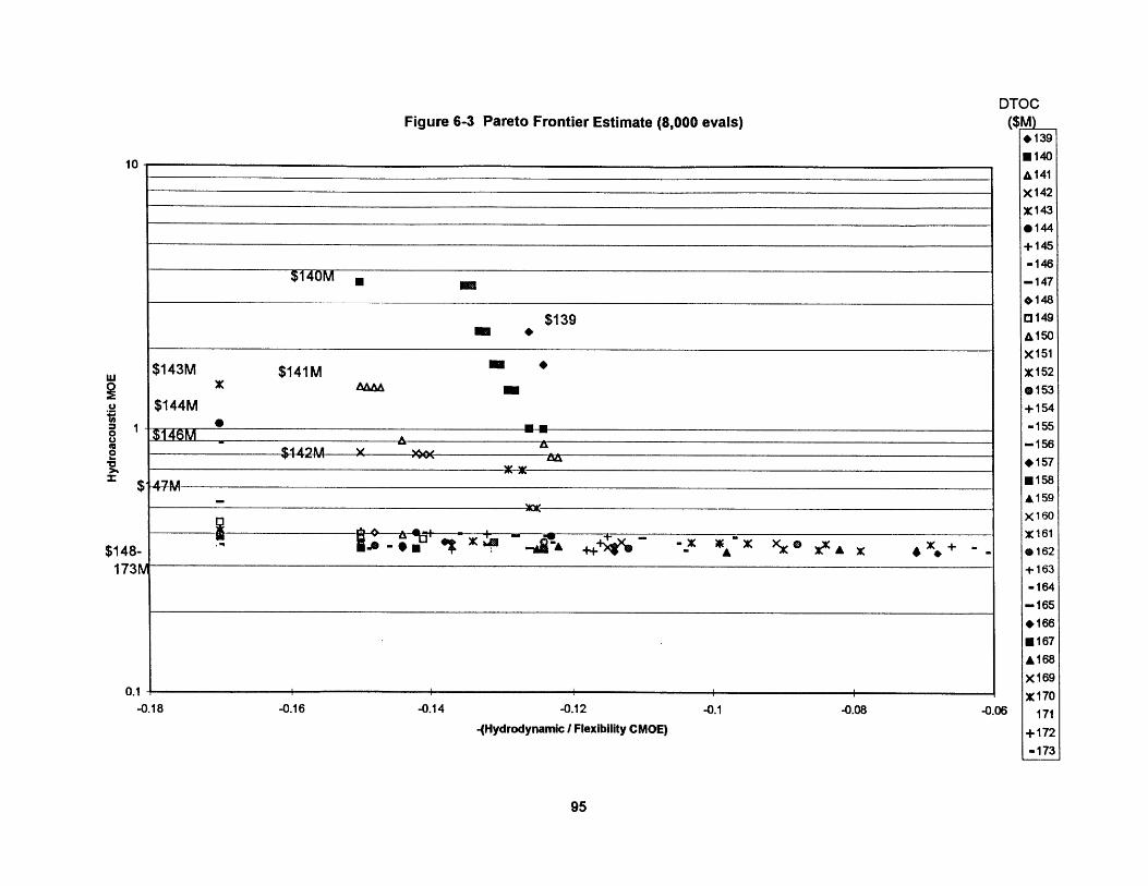
Figure 6-3 Pareto Frontier Estimate (8,000 evals)
$140M * -
$139
$143M $141M
$144M
$146M
$142M X
$ 47M
r .6 - - =
-X X X X-AA
8 -0.14 -0.12
-(Hydrodynamic I Flexibility CMOE)
-0.16
$148-173K11
DTOC($M
* 139
S140
A 141X 142X 1430144
+145
-146-147*1480149A 150
X 151X152@153+154
-155
-156*157
0158
A159
X 160
X 161
@162
+163
-164
-165
* 166S167
A 168
X 169K 170
06 171
+172-173
0.1 i-0.1 -0.08 -0.
I I I I i
-s~ ~xsl
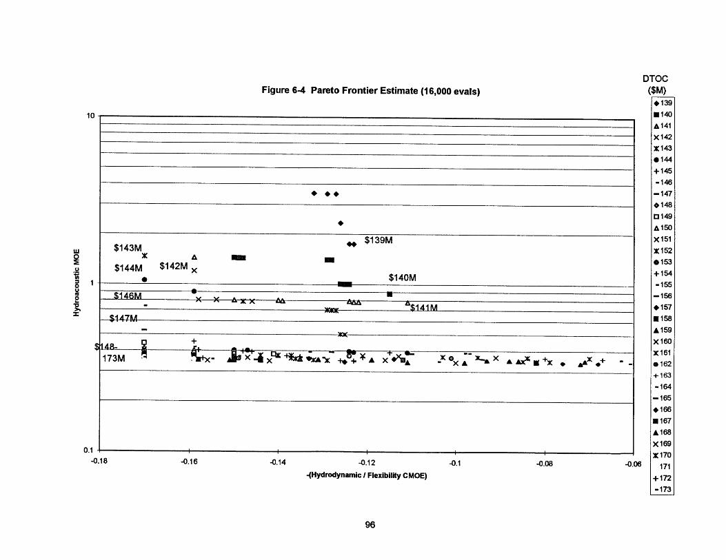
DTOCFigure 6-4 Pareto Frontier Estimate (16,000 evals) ($M)
* 13910 10140
A141
X 142
X143
e144
+145
-146
* * * -147
*148
0149
A 150
$139M X 151$143M X 152
A - - 0153. $144M $142M $140M +153
$140M +1541 -155
$146M -,,5 -is146M "Y " '&$141M *157
S $147M *0158
A 159+ X160
$-4 8 .- A X161173M x ANS. X X AhX+X X .pAOAX& A X162
+163
-164
-165
*166
N 167
A168
X 1690.1
X 170-0.18 -0.16 -0.14 -0.12 -0.1 -0.08 -0.06 171
-(Hydrodynamic I Flexibility CMOE) +172
-173
96
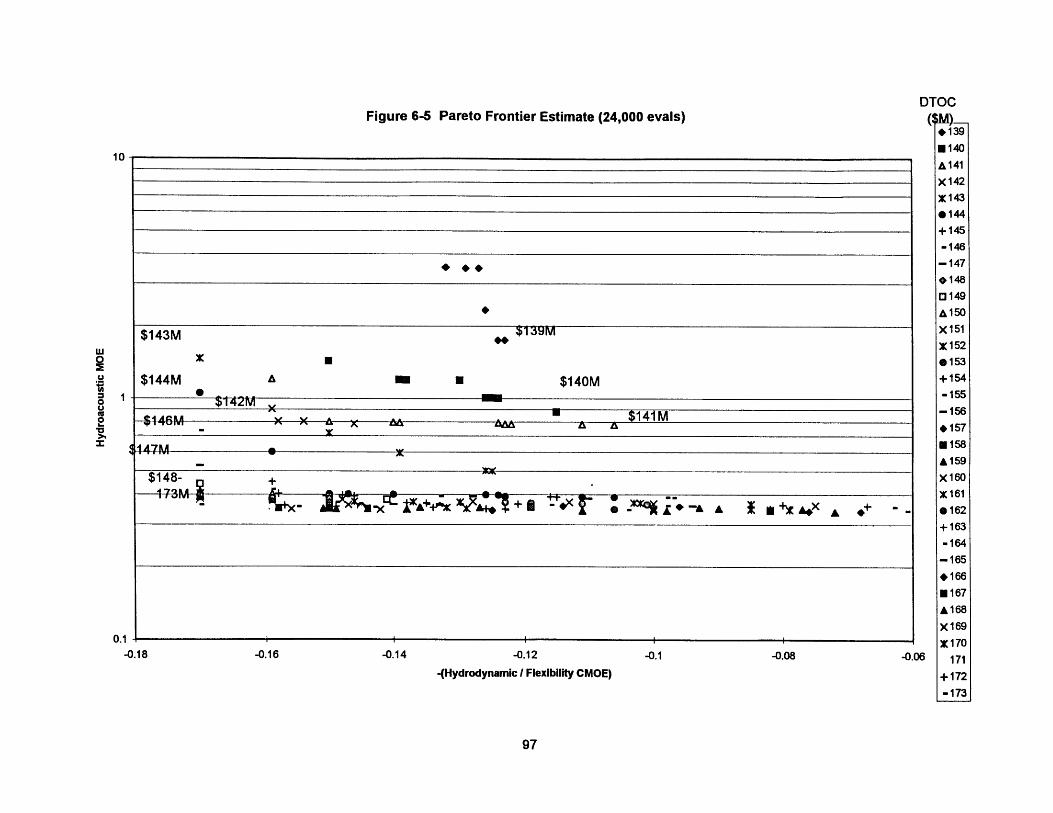
DTOCFigure 6-5 Pareto Frontier Estimate (24,000 evals) (M
1391040
A 141
X142S143
8144
+145-146-147*148
0149A150
O X 153
2 $144M A - $140M +154$42M ma -155
2 ,14 - ". ,, $141M 1560 X A $141 M
S 147M x 158A 159
$148- + I160y+X- gb~r L tr ; 5 A *+(.X +X161
o -;K *- -+"- 0 -A, A A* ( A @162+163-164
-165
#166
N167
A168
X1690.1 I I I I I170
-0.18 -0.16 -0.14 -0.12 -0.1 -0.08 -0.06 171-(Hydrodynamic I Flexibility CMOE) +172
-173

DTOCFigure 6-6 Pareto Frontier Estimate (32,000 evals) ($M)
* 139
10 E140
A 141
x 142
X143
e144
+145
-146
* * * -147
0 148
01490 A150
$1,39M X151$143M 152
Se152
e 153
$144M $142 $140M +1541- -155
-156$14M $141M -1566 X X L Y 1 5 7
S $47M e 158
- 159$148- + x 16o
173 1 I- I A' . • +A -" :" jAA - X161• L+X-A A I ->5eX+ i XpOAA f" .A- 0162
+163
-164
-165
*166
S167
A 168
X 1690.1 170
-0.18 -0.16 -0.14 -0.12 -0.1 -0.08 -0.06 171-(Hydrodynamic I Flexibility CMOE) +172
-173
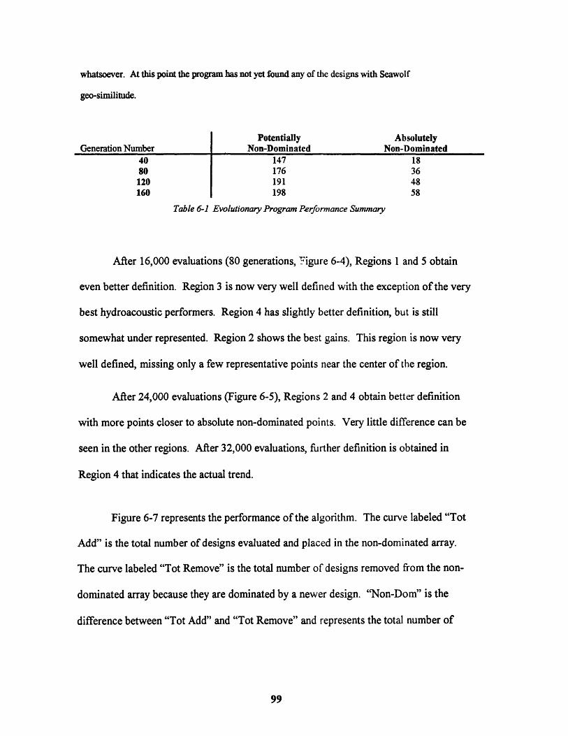
whatsoever. At this point the program has not yet found any of the designs with Seawolf
geo-similitude.
Potentially AbsolutelyGeneration Number Non-Dominated Non-Dominated
40 147 1880 176 36
120 191 48160 198 58
Table 6-1 Evolutionary Program Performance Summary
After 16,000 evaluations (80 generations, Figure 6-4), Regions 1 and 5 obtain
even better definition. Region 3 is now very well defined with the exception of the very
best hydroacoustic performers. Region 4 has slightly better definition, but is still
somewhat under represented. Region 2 shows the best gains. This region is now very
well defined, missing only a few representative points near the center of the region.
After 24,000 evaluations (Figure 6-5), Regions 2 and 4 obtain better definition
with more points closer to absolute non-dominated points. Very little difference can be
seen in the other regions. After 32,000 evaluations, further definition is obtained in
Region 4 that indicates the actual trend.
Figure 6-7 represents the performance of the algorithm. The curve labeled "Tot
Add" is the total number of designs evaluated and placed in the non-dominated array.
The curve labeled "Tot Remove" is the total number of designs removed from the non-
dominated array because they are dominated by a newer design. "Non-Dom" is the
difference between "Tot Add" and "Tot Remove" and represents the total number of

designs in the non-dominated array. "Absolute Non-Dom" represents the number of non-
dominated designs from the exhaustive search found by the evolutionary program.
TR
-Abesde NonDan
i0 Total Absolutely
a" ! Non-Doninated0
0 8000 16000 24000 3;E
Number of Evaluations
Figure 6-7 Evolutionary Program Performance
During the initial generations, the number of non-dominated solutions increases
rapidly because the number of previously found designs is small. As more non-
dominated designs are added, the rate of finding new non-dominated designs drops off.
The number of absolutely non-dominated designs behaves in a similar manner, but is not
as pronounced. The marginal gain in conducting further evaluations continues to drop off
as more designs are evaluated. Even though only a small fraction of the absolutely non-
dominated designs have been found (20% after 160 generations) the extents and trends in
100
attribute space are very well defined. The algorithm has found a large number of designs
that very closely approximate the absolutely non-dominated designs.
6.3 Expanding the Design Parameter Space
There are many discontinuities in the exhaustive search Pareto frontier. The
exhaustive search does not provide a continuous plot for two reasons. First, the
continuous parameters are approximated as discreet. The larger the distance between the
discreet values, the larger the distance between the points in effectiveness space. Second,
even if all continuous parameters were modeled to a high precision, there are still 2
parameters that are by their very nature discreet: sonar type and battery type. To reduce
the distance between the points on the Pareto frontier, the number of binary digits in each
continuous gene is increased by one in the next phase of the search.
If the minimum and maximum values for design parameters are improperly
chosen, the solution space can be arbitrarily constrained. In this problem 29% of all non-
dominated variants have a battery power at the minimum value and only dominated
variants have hull diameters less than 10 feet. This indicates that the low end of battery
power was improperly chosen, arbitrarily constraining the solution to the larger hulls that
can support the larger battery power requirements. In addition, only dominated solutions
have battery power greater than 5100 kWe, indicating that the maximum battery power of
6500 kWe is too high. The battery power range is lowered for the next phase of the
search.
A similar phenomenon occurred with coating thickness. Of all non-dominated
designs, 86% have the maximum coating thickness allowed. This again indicates that the
101
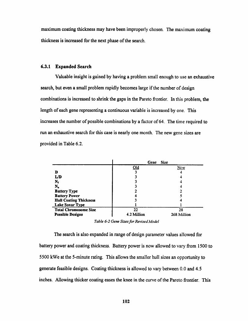
maximum coating thickness may have been improperly chosen. The maximum coating
thickness is increased for the next phase of the search.
6.3.1 Expanded Search
Valuable insight is gained by having a problem small enough to use an exhaustive
search, but even a small problem rapidly becomes large if the number of design
combinations is increased to shrink the gaps in the Pareto frontier. In this problem, the
length of each gene representing a continuous variable is increased by one. This
increases the number of possible combinations by a factor of 64. The time required to
run an exhaustive search for this case is nearly one month. The new gene sizes are
provided in Table 6.2.
Gene SizeOld New
D 3 4L/D 3 4Nf 3 4N, 3 4Battery Type 2 2Battery Power 4 5Hull Coating Thickness 3 4Lake Sonar Type 1 1Total Chromosome Size 22 28Possible Designs 4.2 Million 268 Million
Table 6-2 Gene Sizes for Revised Model
The search is also expanded in range of design parameter values allowed for
battery power and coating thickness. Battery power is now allowed to vary from 1500 to
5500 kWe at the 5-minute rating. This allows the smaller hull sizes an opportunity to
generate feasible designs. Coating thickness is allowed to vary between 0.0 and 4.5
inches. Allowing thicker coating eases the knee in the curve of the Pareto frontier. This
102
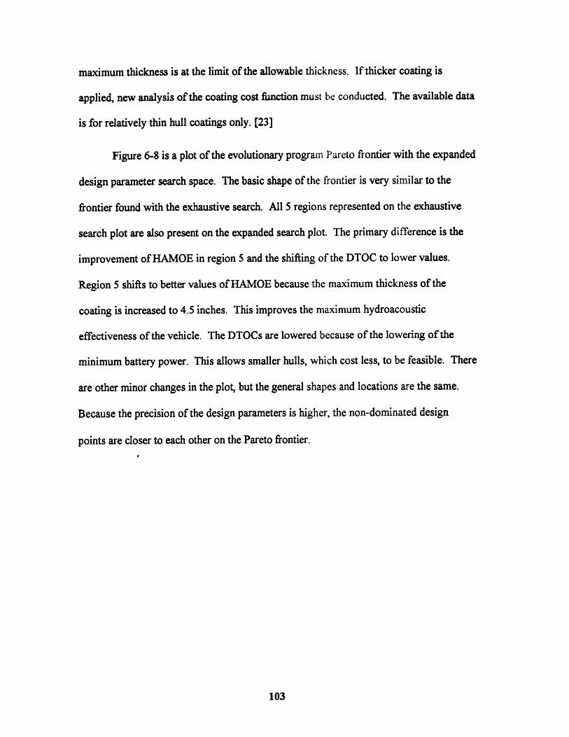
maximum thickness is at the limit of the allowable thickness. If thicker coating is
applied, new analysis of the coating cost function must be conducted. The available data
is for relatively thin hull coatings only. [23]
Figure 6-8 is a plot of the evolutionary program Pareto frontier with the expanded
design parameter search space. The basic shape of the frontier is very similar to the
frontier found with the exhaustive search. All 5 regions represented on the exhaustive
search plot are also present on the expanded search plot. The primary difference is the
improvement of HAMOE in region 5 and the shifting of the DTOC to lower values.
Region 5 shifts to better values of HAMOE because the maximum thickness of the
coating is increased to 4.5 inches. This improves the maximum hydroacoustic
effectiveness of the vehicle. The DTOCs are lowered because of the lowering of the
minimum battery power. This allows smaller hulls, which cost less, to be feasible. There
are other minor changes in the plot, but the general shapes and locations are the same.
Because the precision of the design parameters is higher, the non-dominated design
points are closer to each other on the Pareto frontier.
103
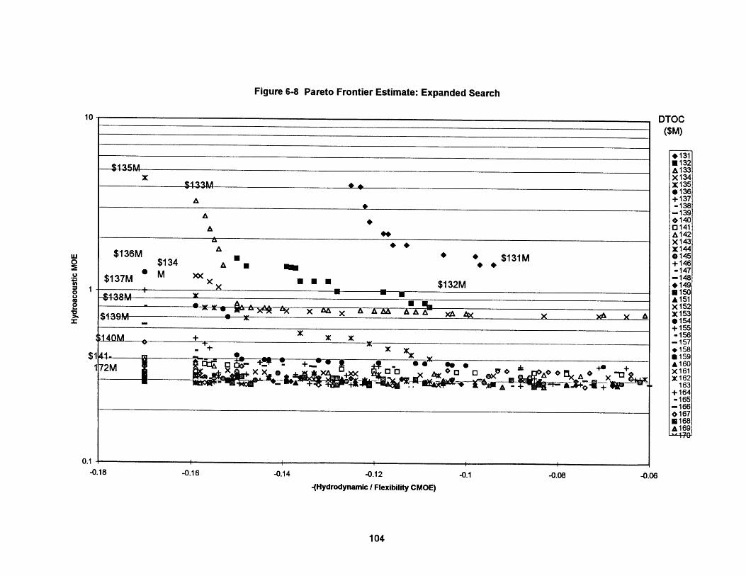
Figure 6-8 Pareto Frontier Estimate: Expanded Search
10 DTOC($M)
*131$132A133
X x134$133M . X 135
o136A +137-138
A -13901400141
*,& 142X1423
a r144S $136M * $131M 0145
8$134 +146
$137M M o< -147$137M x $132M 149$138M -A151
0154+155
X -156S140M + -157* 158
+ 164
-165-1660167168S169
0.1-0.18 -0.16 -0.14 -0.12 -0.1 -0.08 -0.06
-(Hydrodynamic I Flexibility CMOE)
104
6.4 Focused Search
There are areas on the expanded search plot where the separation between points
is larger than desired. For example, the area bounded by HAMOE between 0.6 and 1.7
and HD/F CMOE between -0.16 and -0.14 appears to contain several knees in curves and
has fairly wide separation. To focus in on this region, all the points within the region are
analyzed separately from the remainder of the frontier. The minimum and maximum
values of the design parameters within this region are used as the minimum and
maximum design parameters for a new search. The search starts with the non-dominated
designs found in the expanded search. The results of this focused search are presented in
Figure 6-9.
The area of the focused search now has a much higher density of non-dominated
points. The frontier in this region has also improved, especially for those designs with a
DTOC of $133 million and $134 million. The frontier for these costs has improved HD/F
CMOE.
105
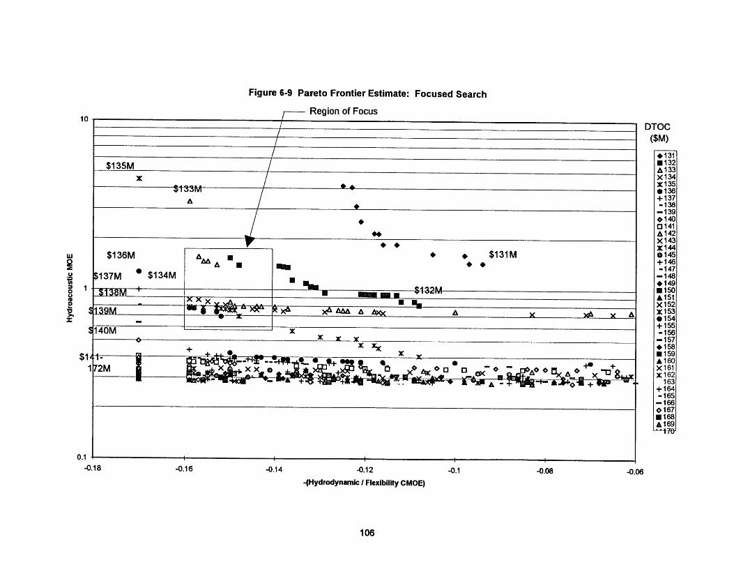
Figure 6-9 Pareto Frontier Estimate: Focused Search
-- Region of Focus
uw 130M A VI0
. $137M $134M
$138M ._ .....X X
$140M X
$11>., X
0.1
-0.18 -0.16 -0.14 -0.12 -0.1 -0.08
-(Hydrodynamic I Flexibility CMOE)
DTOC($M)
*131- 132A 133X 134Xr135
- *136+137-138
--139*1400141A 142
- X143X1440145+146-147
-148*1490150-A151X 52
S X1530154+155S -156-157* 1580159A 160X161X 162
163+164-165-166
-0 167
-0.06
106
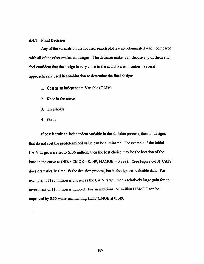
6.4.1 Final Decision
Any of the variants on the focused search plot are non-dominated when compared
with all of the other evaluated designs. The decision-maker can choose any of them and
feel confident that the design is very close to the actual Pareto frontier. Several
approaches are used in combination to determine the final design:
1. Cost as an independent Variable (CAIV)
2. Knee in the curve
3. Thresholds
4. Goals
If cost is truly an independent variable in the decision process, then all designs
that do not cost the predetermined value can be eliminated. For example if the initial
CAIV target were set to $136 million, then the best choice may be the location of the
knee in the curve at (HD/F CMOE = 0.149, HAMOE = 0.398). (See Figure 6-10) CAIV
does dramatically simplify the decision process, but it also ignores valuable data. For
example, if $135 million is chosen as the CAIV target, then a relatively large gain for an
investment of $1 million is ignored. For an additional $1 million HAMOE can be
improved by 0.35 while maintaining ID/F CMOE at 0.149.
107
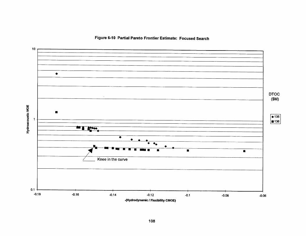
Figure 6-10 Partial Pareto Frontier Estimate: Focused Search
I-
/% ~ ..e E a
Knee in the curve
I I I I
-0.16 -0.14 -0.12
-(Hydrodynamic I Flexibility CMOE)
-0.08
108
-0.18
DTOC($M)
1 1361
-0.06
Goals and thresholds are better means of bracketing the decision process if
needed. For example, it may be decided that HAMOE should be less than 0.8 to ensure
that the uncertainty band is small enough for proper propulsor evaluation. Setting the
HAMOE threshold at 0.8 eliminates all designs above this value. The decision of goal
and threshold for HD/F CMOE is actually one of what geo-similitude is desired. To
achieve a HD/F CMOE greater than 0.15, Seawolf or New Attack geo-similitude must be
used. All designs between 0.15 and 0.16 are Seawolf while all those at 0.17 are New
Attack.
If geo-sim is not very important, then the best choice may be the design at the
knee in the curve for $136 million. If Seawolf geo-sim is important, then any of the
designs with HD/F CMOE at 0.16 is the appropriate choice because of the flatness of the
curve in this region. The trade-off in this situation is strictly HAMOE vs. DTOC. If New
Attack geo-sim is important, then any of the designs with HD/F CMOE equal to 0.17 is
appropriate and a direct trade-off of HAMOE vs. DTOC is used.
109
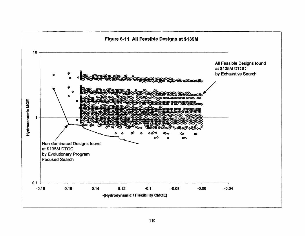
Figure 6-11 All Feasible Designs at $135M
All Feasible Designs foundat $135M DTOCby Exhaustive Search
o o(Poo 00
000
Non-dominated Designs foundat $135M DTOCby Evolutionary ProgramFocused Search
-0.12 -0.1
-(Hydrodynamic / Flexibility CMOE)
110
0O
wO
oU0o
-r0o
0.1 4--0.18 -0.16 -0.14 -0.08 -0.06 -0.04
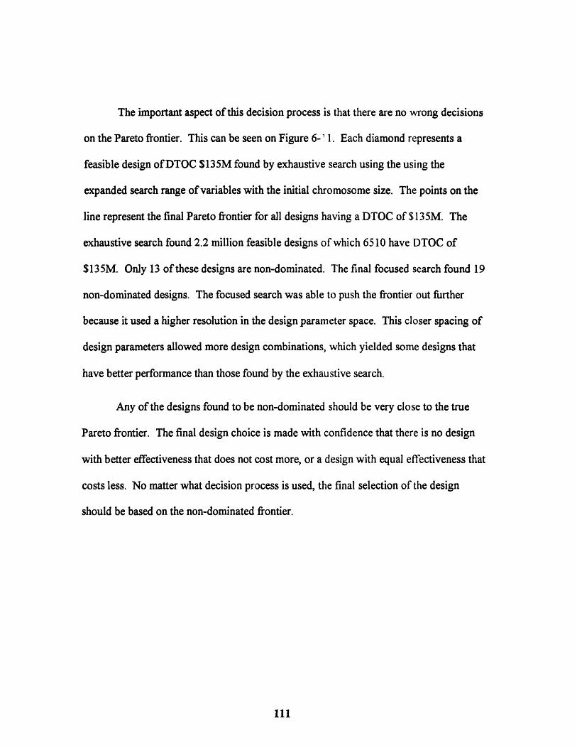
The important aspect of this decision process is that there are no wrong decisions
on the Pareto frontier. This can be seen on Figure 6-' 1. Each diamond represents a
feasible design of DTOC $135M found by exhaustive search using the using the
expanded search range of variables with the initial chromosome size. The points on the
line represent the final Pareto frontier for all designs having a DTOC of $135M. The
exhaustive search found 2.2 million feasible designs of which 6510 have DTOC of
$135M. Only 13 of these designs are non-dominated. The final focused search found 19
non-dominated designs. The focused search was able to push the frontier out further
because it used a higher resolution in the design parameter space. This closer spacing of
design parameters allowed more design combinations, which yielded some designs that
have better performance than those found by the exhaustive search.
Any of the designs found to be non-dominated should be very close to the true
Pareto frontier. The final design choice is made with confidence that there is no design
with better effectiveness that does not cost more, or a design with equal effectiveness that
costs less. No matter what decision process is used, the final selection of the design
should be based on the non-dominated frontier.
111

(This Page Intentionally Blank)
112

7Conclusion
This thesis proposed use of evolutionary programs to generate non-dominated
Pareto frontiers for complicated multi-objective design problems. The method was
demonstrated to work on an application to Large Scale Vehicle II.
A need exists for a tool capable of searching a large number of potential designs
in concept development. Both New Attack Submarine (NSSN) and next generation
aircraft carrier (CVX) evaluated only a very small fraction of the potential concept
designs. A great deal of faith was placed in the ship designers to optimize the design, but
only a small number of designs were evaluated in formal studies. The evolutionary
program developed in this thesis can be applied in a relatively straight forward manner to
full scale ship and submarine development. The framework developed in Chapter 3 is
very general in nature, and can be applied to any multi-objective design problem. Only
the objective attributes and design parameters need be changed.
The evolutionary program is very robust in its search for the Pareto frontier. It is
designed to conduct a search that both explores and exploits the design space at the same
time. The search method is simple and straight forward to implement. There are many
variables that affect the performance of the genetic algorithm, but as long as the variables
selected are reasonable, the evolutionary program does well in finding the Pareto frontier.
Experimentation to optimize the search program can improve its performance, but any
form of the algorithm performs reasonably well.
113

A new method, multi-attribute iso-effectiveness (MAIE), was proposed to
generate combined measures of effectiveness (CMOE) using expert opinion.
Unfortunately, not enough data was collected to make a preliminary judgment on the
accuracy of this method. The method has a major drawback in that it is very question
intensive and requires a significant amount of time from the expert to complete. Because
of this, it can only be used to combine 3 or 4 attributes at most. Perhaps this method
could be used on a small scale problem to compare responses received from experts using
one of the other methods to construct CMOEs discussed in Chapter 3.
If any expert opinion method is used to create an CMOE, extreme care must be
used in selecting the parameters (MOEs or MOPs) to combine and the goals and
thresholds associated with these parameters. If this initial step is performed improperly,
then the rest of the decision analysis is useless. In this thesis, a CMOE was created for
hydrodynamic and flexibility. The goals and thresholds selected were based on expert
opinion, but it may have been better to re-select the variables and their ranges after initial
evaluations. One of the MOPs (number of Froude scale maximum speed runs) did not
enter into the decision process at all because all of the non-dominated designs exceeded
the goal. Geo-similitude was used as a MOP because it adds value when the model is
used to obtain data on current or proposed full-scale submarines. When this MOP was
disregarded, no variants with geo-similitude were found on the Pareto frontier. This
indicates that if LSV II is being built to assist in development of near-term submarines,
then one with geo-similitude should be built. If, on the other hand, LSV II is being built
for long-term research, the geo-similitude of future submarines should be built. This
114
research suggests that a "short, fat" model may be the best option as a prototype for
submarines of the future.
Risk was not directly addressed in this thesis, but it can be integrated into the
method in one of three ways. It can be treated as a separate objective attribute. Each
concept in the design parameter space can be evaluated for risk based on an scale from
high to low and the results for all design parameters summed to give a final risk score. If
combining certain design parameters either increases or decreases risk, this can be
reflected in the final risk score. Another possible method is to combine risk with the cost
objective attribute. High risk design characteristics can be assigned a higher cost to
offset the risk. A third possible method is to assign each objective attribute an expected
range of values. Predicting cost, performance and effectiveness is not always an exact
science, and each of these parameters have some uncertainty associated with them. If this
uncertainty can by quantified and carried through the problem, then risk can be
represented on the Pareto frontier graph as an ovoid around the expected value of
objective attributes.
The evolutionary program has been shown to work in a relatively simple
submarine model, and should be applicable to full scale ship and submarine concept
design. It provides a structured and efficient method for searching design space to obtain
the set of non-dominated designs for presentation to the decision-maker. This allows the
decision-maker to select one or more of the non-dominated designs for further design.
No matter what search method is used, the Pareto frontier should be the starting place for
decision makers. Evolutionary programs provide this capability.
115

(This Page Intentionally Blank)
116
Bibliography
1. Thurston, Deborah L., "A Formal Method for Subjective design Evaluation withMultiple Attributes", Research in Engineering Design, Springer-Verlag New York, Inc.,1991.
2. Michalewicz, Zbigniew, Genetic Algorithms + Data Structures = Evolution Programs,Springer-Verlag, 1992.
3. Thomas, M., "A Pareto Frontier for Full Stern Submarines via Genetic Algorithm",Ph.D. Thesis, Massachusetts Institute of Technology, June 1998.
4. Lamb, J.A. (Large Scale Vehicle Design Manager, Newport News Shipbuilding),"LSV2 Concept Deliverables", May 23, 1997.
5. Thomas, G., Personal Interview, Naval Sea Systems Command, August, 1997.
6. "NSSN Cost and Operational Effectiveness (COEA) Report for Milestone II", Centerfor Naval Analysis (CNA), July 1993.
7. "NSSN Cost and Operational Effectiveness Report", Naval Underwater WarfareCenter (NUWC) Newport, Rhode Island, May 1995.
8. Cohen, J., NSSN Milestone II COEA Director, Personal Interview, Newport, RhodeIsland, September, 8, 1997.
9. Manvel, T., Moore, K., Lillard, J., Bouchoux, D., Perin, D., Raber, J., "CVXRequirements Day Presentation", Naval Surface Warfare Center, Carderock, October 1,1997.
10. Executive Office of the President, Office of Management and Budget, Circular No.A-94, "Guidelines and discount Rates for Benefit-Cost Analysis of Federal Programs",October 29, 1992.
11. Hockberger, W.A., "Total System Ship Design in a Supersystem Framework", NavalEngineers Journal, pp 147-166, May, 1996.
12. Whitcomb, C.A., "Naval Ship Design Philosophy Implementation", Naval EngineersJournal, January, 1998.
13. Brown, A. and Thomas, M., "Reengineering the Naval Ship Concept DesignProcess", Draft Paper for "From Research to Reality in Ship systems Engineering",ASNE, September 18-19, 1998.
117
14. de Neufville, Richard, Applied Systems Analysis Engineering Planning andTechnology Management, McGraw Hill, Inc., 1990.
15. Decision Making with Expert Choice, Expert Choice, Inc., Pittsburgh, PA.
16. Jackson, H., Submarine Design Trends, MIT Professional Summer Course, June,1997.
17. Szymborski, Joseph, (Director, Government Programs, GNB Technologies),"Request for Information - Large Scale Vehicle", Memorandum, May 30, 1997.
18. Jebson, G., "Radiated Noise Arrays at Acoustic Research Detachment", Presentation,Naval Sea Systems Command, July, 14, 1997.
19. Cann, G., Sullivan, P., Brooks, R., Reed, J., Introductions to Submarine Design,1995.
20. Jackson, H., Captain, USN, Retired, Personal Interview, Massachusetts Institute ofTechnology April 1, 1998.
21. Harrison, C.E. and White, R.T. (Newport News Shipbuilding, Department E13),"DDM-0330, LSV 2 Project/WBS 313; Endurance", Decision Memorandum, September25, 1997.
22. Sette, K.R., "LSV-2 Total Ownership Cost Model", Report for NR NAVSEA Det122, June 19, 1997.
23. Awwad, S., Wernecker, W., Anwar, S., McKeon, S., Zehner, K., Freeman, R., NHTInstallation Process Cost Elements, Revision 4, Naval Surface Warfare Center,Carderock Division, July 1997.
24. Blake, W., "Large Scale Vehicle Acoustic Performance and Radiated Noise Arrays",Memorandum to Spina, J. and Thomas, G., July 3, 1997.
25. Millet, Ido, and Saty, Thomas L., "Selecting a Synthesis Mode in the AnalyticalHierarchy Process", ISAHP 1996, Vancouver, Canada, July 12-15, 1996.
26. Shahak, S., "Naval Ship Concept Design: An Evolutionary Approach", Master ofScience Thesis, Massachusetts Institute of Technology, February 1998.
118
Appendix A: Expert Opinion Surveys
The final 6 pages of this appendix contain the two surveys proposed to obtain
expert opinion on hydrodynamic and flexibility combined measures of effectiveness. The
first survey uses the Analytical Hierarchy Process (AHP), and the second survey uses
multi-attribute iso-effectiveness (MAIE). The survey refers to the MAIE method as
"Multi-Attribute Value Analysis". The name of the method was changed to MAIE after
the survey was distributed to avoid confusion with a method proposed by Brown[13].
Survey response was not as good as initially hoped. The results from this thesis
are based entirely on the author's responses to the survey. A minimal amount of analysis
was performed with the data available. The graph on the following page represents this
analysis effort.
The basis of the graph is the set of iso-effectiveness curves developed from the
MAIE method. The bold lines represent the MAIE method iso-effectiveness curves.
"Iso-effectiveness" curves were developed for the AHP method by ranking the points
evaluated in the AHP survey. The numbers in the field of the plot are the rankings of that
point. For example, by the AHP survey, the ranking of number of Froude scale
maximum speed runs (FSRs) equal to 8 and margin equal to 9% is 7 out of 16. There are
16 points on this graph evaluated by AHP. The "AHP iso-effectiveness" lines are drawn
as the light curves and only represent possible iso-effectiveness curves. They are drawn
so that between any two curves there is only one of the points evaluated in the AHP
method. There are not two points between two curves, because then another iso-
119

effectiveness curve could be drawn between them that represents the effectiveness of a
value in-between the two points.
If the two methods were completely consistent, then the AHP curves would never
cross the MAIE curves. This is not consistently the case, as can be seen in the lower right
hand corner. AHP point 11 is on an MAIE curve, yet points 12 and 13 are above this
curve. By AHP Point 11 has better effectiveness and by MAIE, points 12 and 13 have
better effectiveness.
For most of the design space of this specific example, both methods are
consistent. In this one region, however, the two methods disagree. There is not enough
data available to determine the reasons for the discrepancies. Further research is needed
in this area to determine which method, if any, reflects the expert's true opinion on the
topic.
120

Iso-effectiveness Curves for MAIE and AHPS with Geo-sim constant
Froude Scale Runs
121
12%
LSV Hydrodynamic / Flexibility Survey
In this thesis, the LSV design is structured as a multi-attribute decision problem. Threeoverall attributes are typically the maximum number which can be consideredsimultaneously by a decision maker. The 3 attributes chosen for this design are cost,hydrodynamic effectiveness and hydro-acoustic / flexibility effectiveness.
The hydro-acoustic and flexibility attribute involves more than one performance metric.Expert opinion must be used to establish and synthesize the relative value of 3performance variables: Number of Runs at Froude Scale Speed, Margin and Geo-similitude. Two methods of collecting this expert opinion are being investigated: Multi-Attribute Value Analysis and Analytical Hierarchy Process (AHP).
Both methods require the determination of goals and thresholds for each variable. Afterdiscussions with LCDR Greg Thomas, I have chosen the following goals and thresholds:
Number of Runs at Froude Scale Speed that can be performed on one battery charge.Goal = 10, Threshold = 7
Amount of margin that is available for future growth, including propulsor installation.Goal = 12%, Threshold = 3% (Variant Al currently has a value of 6.3%)
The type of geo-similitude that is chosen.Options: NSSN, SSN-21, None (i.e. has "submarine-like shape")
Goals represent the highest value the decision maker believes to be obtainable with thetechnology available in the time frame of the project, or the value at which furtherimprovement no longer adds significant improvement to the project. Thresholds are thevalue of minimum acceptable performance. Below this value, it is not worth continuingwith the project.
If a member achieves values above the goal, no additional credit is given. It is treated thesame as if it had only achieved the goal. If any value is below the threshold, the LSV isassumed to be not feasible. If you do not agree with the variables chosen here, or thegoals or thresholds, I would appreciate any feedback you could provide. Obviously, ifthis first step of the process is flawed, the remainder of the process will not givemeaningful results.
The input required for the Multi-Attribute Value Analysis is obtained by the expertanswering a set of questions to generate a set of iso-effectiveness curves. For example, ifone of the variables is held constant, how much change is required in each of the tworemaining variables to give equal effectiveness? Specifically, if geo-similitude is heldconstant, what value of margin combined with 9 Froude Scale Runs gives equaleffectiveness to 10 Froude Scale Runs and 3% margin? If this question is difficult toanswer initially, the expert might try to bracket the answer until equivalence point isreached. For example, 12% margin is probably preferred, but 3.5% is probably not. Theattached EXCEL file gives the complete survey along with an automatic plot of iso-effectiveness lines.
122
The second method uses AHP and requires that the expert to make a set of pair-wisecomparisons using a questionnaire. First the relative importance of each of the variables iscompared. Specifically, the expert must compare Geo-sim to Margin, Geo-sim to Numberof Froude Scale Runs, and Margin to Number of Froude Scale Runs. Each of the specificvalues under each category ure then compared to each other specific value within itscategory. All comparisons are on a scale from 1 to 9, with 1 indicating the choices areequal and 9 indicating that one option is extremely much more important than the other.
There are no correct or incorrect answers to these questions. The value is in obtaininginput from the expert decision makers. From my own experience, filling out these types ofsurveys can be difficult and confusing. I have attempted to make the process as easy aspossible, but any feedback you can provide would be much appreciated. If you have anyquestions or feedback, I can be reached at email [email protected] or phone (617) 253-5317. Thank you very much for your time and input.
123
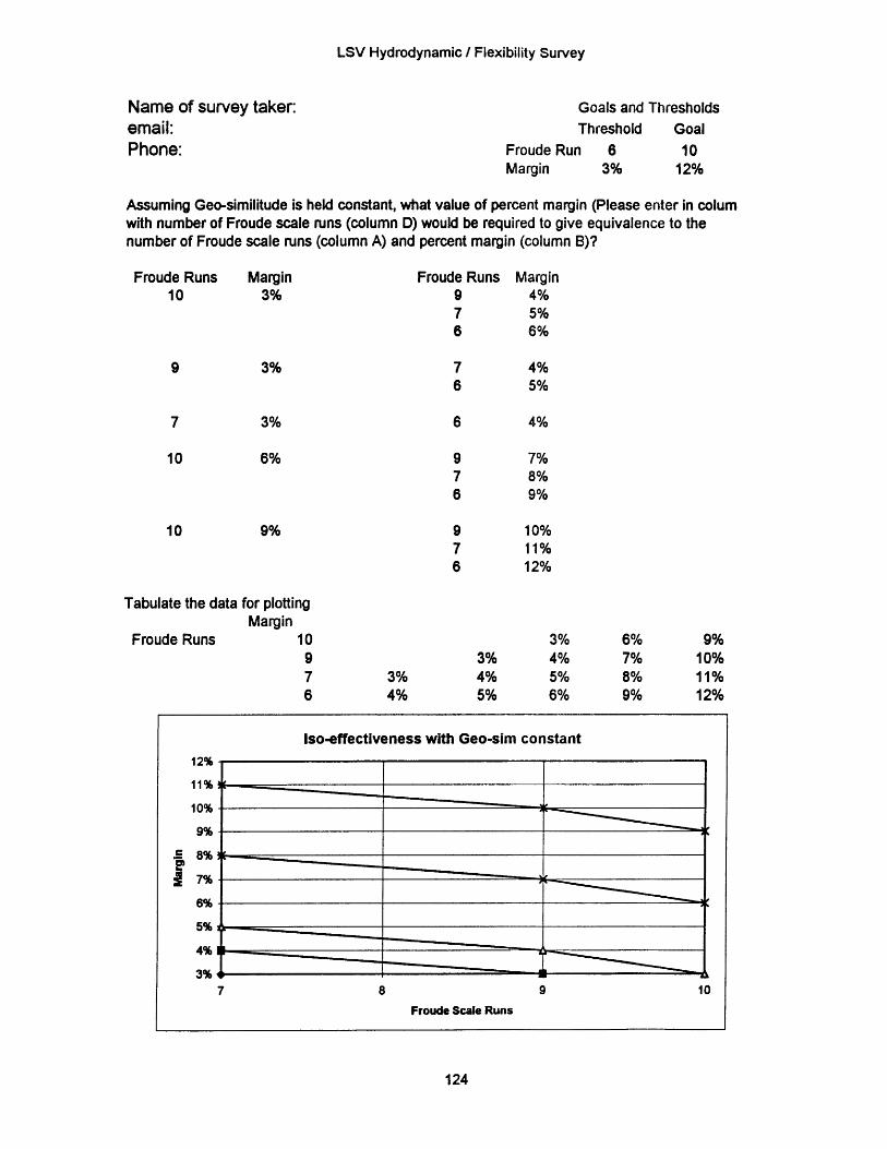
LSV Hydrodynamic / Flexibility Survey
Name of survey taker:email:Phone:
Goals and ThresholdsThreshold Goal
Froude RunMargin
63%
1012%
Assuming Geo-similitude is held constant, what value of percent margin (Please enter in columwith number of Froude scale runs (column D) would be required to give equivalence to thenumber of Froude scale runs (column A) and percent margin (column B)?
Froude Runs10
9
7
Margin3%
Froude Runs97
3%
3%
6%
9%
Tabulate the data
Froude Runs
for plottingMargin
3%4%
3%4%5%
124
Margin4%5%6%
4%5%
4%
7%8%9%
10%11%12%
3%4%5%6%
6%7%8%9%
9%10%11%12%
Iso-effectiveness with Geo-sim constant12%
11%
10%
9%
f 7%
6%
5% ]
4%
3%7 8 9 10
Froude Scale Runs
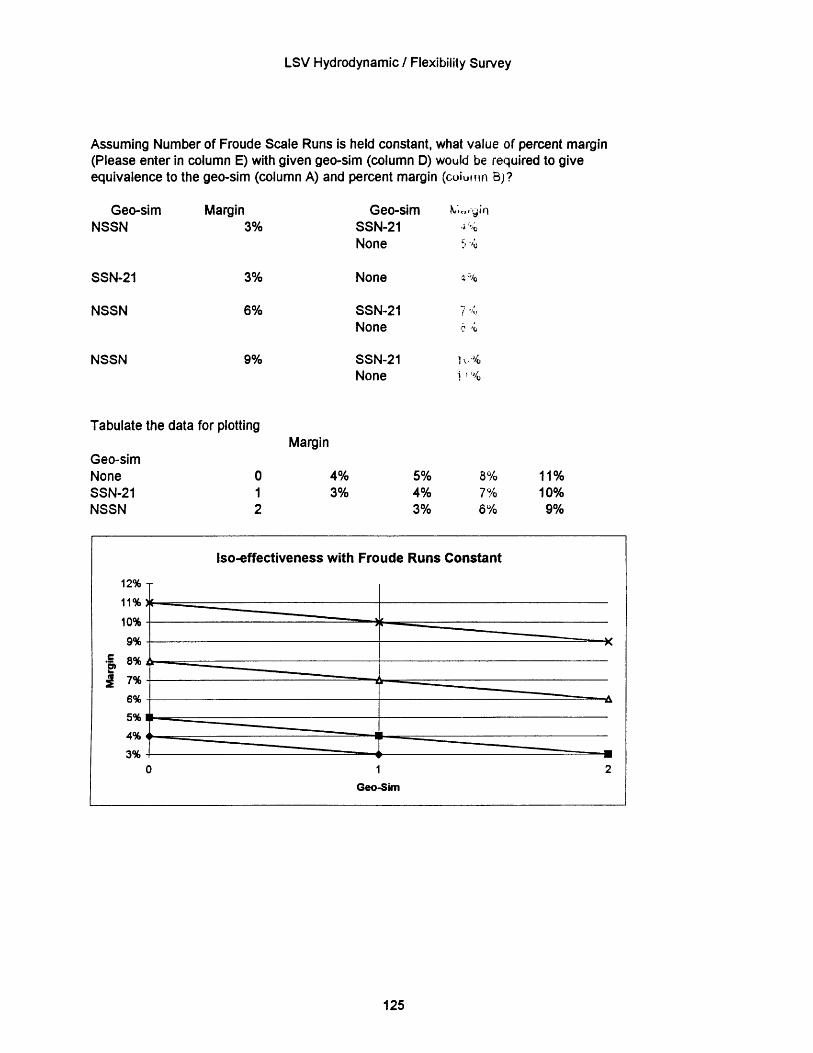
LSV Hydrodynamic / Flexibility Survey
Assuming Number of Froude Scale Runs is held constant, what value of percent margin(Please enter in column E) with given geo-sim (column D) would be required to giveequivalence to the geo-sim (column A) and percent margin (coiumrn B)?
Geo-simNSSN
SSN-21
NSSN
NSSN
Margin3%
3%
6%
9%
Tabulate the data for plotting
Geo-simNoneSSN-21NSSN
Geo-simSSN-21None
None
SSN-21None
N; 1
Q ;Ige
7K'
SSN-21None
Margin
4%3%
5%4%3%
8%7%6%
11%10%
9%
Iso-effectiveness with Froude Runs Constant
P~7~I.
Geo-Sim
125
12%
11%
10%
9%
8%
7%
6%
5%
4%
3%
-
)
-
-
a
-
-
"
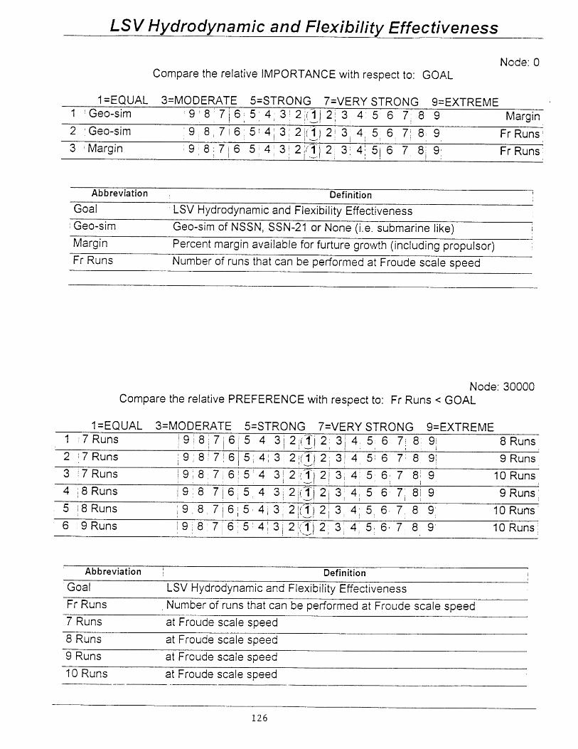
LSV Hydrodynamic and Flexibility Effectiveness
Node: 0Compare the relative IMPORTANCE with respect to: GOAL
1=EQUAL 3=MODERATE 5=STRONG 7=VERYSTRONG 9=EXTREME1 Geo-sim 9 8 7 6: 5 4 3 2(A 2 3 4, 5 6 7, 8 9 Margin
2 Geo-sim 9 8 7 6 5 4 3 2(12 3 4 5 6, 7 8 9 FrRuns3 Margin 9 8 716 5 4 3 2 2 3 4 5 6 7 8 9 FrRuns
Abbreviation Definition
Goal LSV Hydrodynamic and Flexibility EffectivenessGeo-sim Geo-sim of NSSN, SSN-21 or None (i.e. submarine like)Margin Percent margin available for furture growth (including propulsor)Fr Runs Number of runs that can be performed at Froude scale speed
Node: 30000Compare the relative PREFERENCE with respect to: Fr Runs < GOAL
1=EQUAL 3=MODERATE 5=STRONG 7=VERY STRONG 9=EXTREME1 7Runs 9 8 7 6 5 4 3 2 i 2 3 4 56 7 8 9' 8Runs27 Runs 987654321ji 23456789 9Runs
3 7Runs 98 7 6 5 4 3 2( 2 3 41 5 6 7 8 9 10 Runs4 8Runs 9 8 7 6 5 4 32!( 23 45 6 7 8 9 9Runs
5 8Runs 9 8 7 6 5 4 3 2( _) 2 3 4 5 6 7 8 9 10 Runs
6 9Runs 9,8 7 6 5 4 3 2 2 3 4 5 6 7, 8 9 10 Runs
Abbreviation Definition
Goal LSV Hydrodynamic and Flexibility EffectivenessFr Runs Number of runs that can be performed at Froude scale speed
7 Runs at Froude scale speed8 Runs at Froude scale speed9 Runs at Froude scale speed
10 Runs at Froude scale speed
126

LSV Hydrodynamic and Flexibility Effectiveness
Node: 20000
Compare the relative PREFERENCE with respect to: Margin < GOAL
1=EQUAL 3=MODERATE 5=STRONG 7=VERY STRONG 9=EXTREME1 3% 9 8,7 6 5'4 3 2i 121 3 45l 6 7 8 9 6%
2 13% 9 8176 54 3 2' 2 3 4 5 61 7 8 9' 9%'
3 3% 9 8 7615 4 3i2(1 2 3 4 5 6 71 8 9 12%
4 ,6% 9 8 765 4 3 2 ("} 21 3 4i5 6 789 9%
56% 9876543 2 (1 21345 678 9 12%
6 9% 9 8 7 6,5 43 2( 21 3 4. 5 6 7 8' 9 12%
Abbreviation Definition
Goal LSV Hydrodynamic and Flexibility Effectiveness
Margin Percent margin available for furture growth (including propulsor)
3% margin
6% margin
9% margin
12% margin
Node: 10000Compare the relative PREFERENCE with respect to: Geo-sim < GOAL
1=EQUAL 3=MODERATE 5=STRONG 7=VERY STRONG 9=EXTREME1 NSSN 9 8 7 6 5 4 3 2 12 3 4 5 6 7 8 9 SSN-21
2 NSSN 9 8 7 6 5 4 3 2 1:2 3 4 5 6 7 8 9 None
3 SSN-21 9 8 7 6 5 4 3 2 12 3 4 5 6 7 8 9 None
Abbreviation Definition
Goal LSV Hydrodynamic and Flexibility Effectiveness
Geo-sim Geo-sim of NSSN, SSN-21 or None (i.e. submarine like)
NSSN Geo-sim is that of New Attack
SSN-21 Geo-sim is that of USS Seawolf
None Geo-sim is that of a "submarine-like" hull
127

(This page intentionally blank.)
128
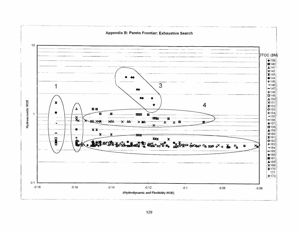
Appendix B: Pareto Frontier: Exhaustive Search
10
wu
0
Pu
0-0 18-01 -0 16 -0 14 -0.12 -0 1 -0.08 -0 06
-(Hydrodynamic and Flexibility MOE)
129
)TOC ($M*139R 140A141X142*1436144+145-146
-14741480149A150X151*1520153+154-155
-156*157
158A159X160*1610162+163-164
-165*1660167Ali68X169*170
171+172
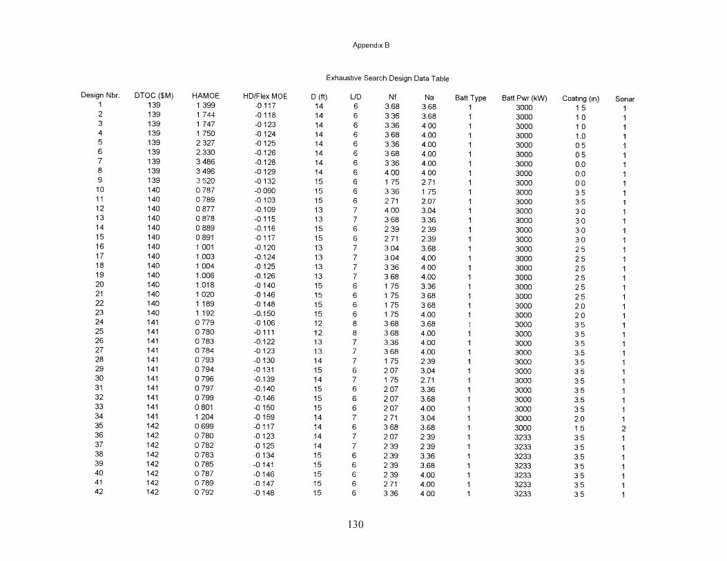
Appendix B
Exhaustive Search Design Data Table
Design Nbr. DTOC ($M) HAMOE HD/Flex MOE D (ft) L/D Nf Na Batt Type Batt Pwr (kW) Coating (in) Sonar1 139 1399 -0117 14 6 3.68 368 1 3000 15 12 139 1744 -0118 14 6 336 3.68 1 3000 10 13 139 1747 -0123 14 6 336 400 1 3000 10 14 139 1750 -0124 14 6 368 4.00 1 3000 1.0 15 139 2327 -0125 14 6 336 4.00 1 3000 05 16 139 2.330 -0.126 14 6 368 4.00 1 3000 05 17 139 3486 -0.128 14 6 336 4.00 1 3000 0.0 18 139 3496 -0129 14 6 400 400 1 3000 0.0 19 139 3520 -0132 15 6 175 271 1 3000 00 110 140 0787 -0090 15 6 336 1 75 1 3000 35 111 140 0789 -0103 15 6 271 2.07 1 3000 35 112 140 0877 -0.109 13 7 400 3.04 1 3000 30 113 140 0878 -0115 13 7 368 3.36 1 3000 30 114 140 0889 -0.116 15 6 239 239 1 3000 30 115 140 0891 -0117 15 6 271 2.39 1 3000 30 116 140 1001 -0.120 13 7 304 3.68 1 3000 25 117 140 1.003 -0.124 13 7 304 4.00 1 3000 25 118 140 1004 -0125 13 7 336 400 1 3000 25 119 140 1.006 -0.126 13 7 368 4.00 1 3000 25 120 140 1.018 -0140 15 6 175 3.36 1 3000 25 121 140 1 020 -0146 15 6 1 75 368 1 3000 25 122 140 1 189 -0148 15 6 175 368 1 3000 20 123 140 1 192 -0.150 15 6 1.75 4.00 1 3000 20 124 141 0779 -0106 12 8 368 3.68 t 3000 35 125 141 0780 -0111 12 8 368 4.00 1 3000 35 126 141 0783 -0.122 13 7 3.36 4.00 1 3000 35 127 141 0784 -0123 13 7 368 4.00 1 3000 3.5 128 141 0793 -0130 14 7 1 75 239 1 3000 35 129 141 0794 -0131 15 6 207 3.04 1 3000 35 130 141 0796 -0.139 14 7 1 75 2.71 1 3000 35 131 141 0797 -0.140 15 6 207 3.36 1 3000 35 132 141 0799 -0.146 15 6 207 3.68 1 3000 3.5 133 141 0801 -0150 15 6 207 4.00 1 3000 35 134 141 1204 -0159 14 7 271 3.04 1 3000 2.0 135 142 0699 -0117 14 6 368 3.68 1 3000 15 236 142 0780 -0123 14 7 207 239 1 3233 3.5 137 142 0782 -0125 14 7 239 239 1 3233 35 138 142 0783 -0134 15 6 239 3.36 1 3233 3.5 139 142 0785 -0141 15 6 239 3.68 1 3233 35 140 142 0787 -0146 15 6 239 4.00 1 3233 35 141 142 0789 -0147 15 6 271 4.00 1 3233 35 142 142 0792 -0148 15 6 336 400 1 3233 35 1
130
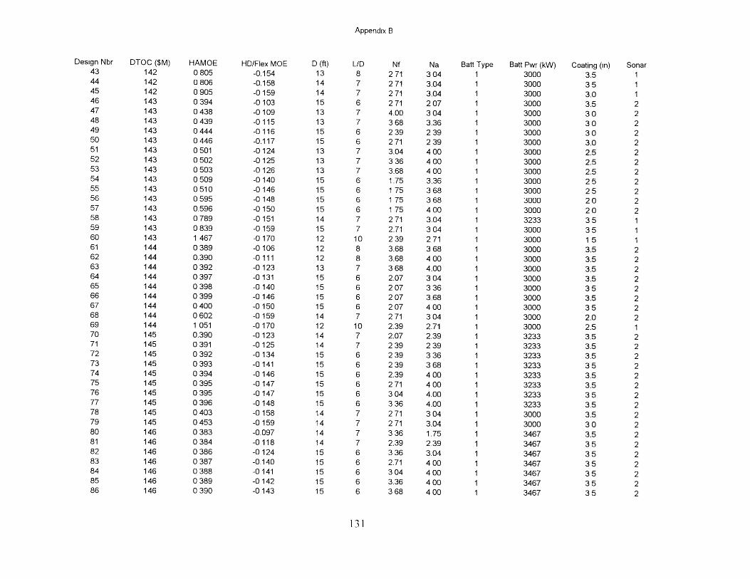
Appendix B
Design Nbr4344454647484950515253545556575859606162636465666768697071727374757677787980818283848586
DTOC ($M)142142142143143143143143143143143143143143143143143143144144144144144144144144144145145145145145145145145145145146146146146146146146
HAMOE0 8050 8060 9050 394043804390 4440 44605010 5020 5030 50905100 5950.5960 7890 8391 4670 3890.3900 392039703980 39904000 6021 0510.3900 3910 39203930 3940 395039503960403045303830 3840 3860 3870 3880 3890 390
HD/Flex MOE-0.154-0.158-0 159-0 103-0 109-0 115-0 116-0.117-0 124-0 125-0 126-0 140-0 146-0148-0 150-0 151-0159-0170-0106-0 111-0 123-0131-0 140-0 146-0 150-0159-0 170-0 123-0 125-0 134-0 141-0 146-0 147-0 147-0 148-0 158-0 159-0.097-0 118-0 124-0.140-0 141-0 142-0 143
D (ft)1314141513131515131313151515151415121212131515151514121414151515151515141414141515151515
Nf2712712712714.003682392713.043363.681.751 751 751 752712.712393.683.683682.072072072072712.392.072392392392.392713043362712713362.393362.713043.36368
Na3043.043.042073043.362392394004004003.363683684003.043042713684004.003043363.684003042.712.392393363684004004.004.003043.041.752.393.04400400400400
Batt Type11111111111111111111111111111111111111111111
Batt Pwr (kW)30003000300030003000300030003000300030003000300030003000300032333000300030003000300030003000300030003000300032333233323332333233323332333233300030003467346734673467346734673467
Coating (In)3.5353.03.53030303.02.52.52.5252520203535153.53.53.53.5353.5352.02.53.53.53.5353.53.5353.53.5303.5353535353535
Sonar11122222222222211122222222122222222222222222
131
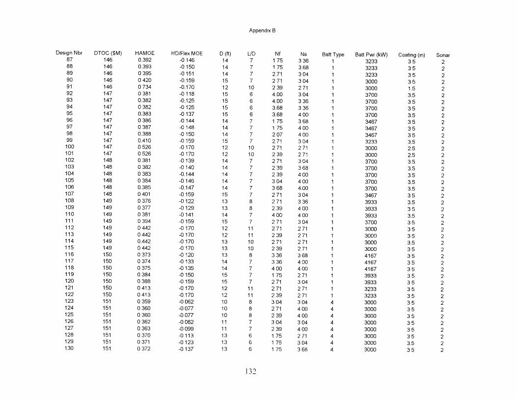
Appendix B
Design Nbr DTOC ($M) HAMOE HD/Flex MOE D (ft) L/D Nf Na Batt Type Batt Pwr (kW) Coating (in) Sonar87 146 0.392 -0146 14 7 175 336 1 3233 35 288 146 0.393 -0150 14 7 175 3.68 1 3233 35 289 146 0395 -0151 14 7 2.71 304 1 3233 35 290 146 0420 -0.159 15 7 271 304 1 3000 35 291 146 0734 -0.170 12 10 239 271 1 3000 1.5 292 147 0381 -0118 15 6 4.00 304 1 3700 3.5 293 147 0.382 -0.125 15 6 4.00 336 1 3700 35 294 147 0382 -0125 15 6 3.68 336 1 3700 35 295 147 0.383 -0137 15 6 3.68 400 1 3700 3.5 296 147 0386 -0144 14 7 1 75 368 1 3467 35 297 147 0387 -0148 14 7 1 75 400 1 3467 35 298 147 0.388 -0150 14 7 207 400 1 3467 35 299 147 0.410 -0159 15 7 2.71 304 1 3233 3.5 2100 147 0526 -0170 12 10 271 271 1 3000 2.5 2101 147 0526 -0170 12 10 239 271 1 3000 2.5 2102 148 0.381 -0139 14 7 271 304 1 3700 3.5 2103 148 0382 -0140 14 7 239 368 1 3700 3.5 2104 148 0383 -0.144 14 7 239 400 1 3700 3.5 2105 148 0384 -0146 14 7 304 400 1 3700 3.5 2106 148 0.385 -0.147 14 7 368 4.00 1 3700 3.5 2107 148 0401 -0159 15 7 271 304 1 3467 35 2108 149 0376 -0122 13 8 271 336 1 3933 3.5 2109 149 0377 -0129 13 8 2.39 400 1 3933 35 2110 149 0381 -0141 14 7 400 400 1 3933 3.5 2111 149 0394 -0159 15 7 271 304 1 3700 35 2112 149 0442 -0170 12 11 2.71 271 1 3000 35 2113 149 0442 -0170 12 11 239 271 1 3000 35 2114 149 0.442 -0170 13 10 271 271 1 3000 3.5 2115 149 0442 -0170 13 10 239 271 1 3000 35 2116 150 0373 -0120 13 8 336 368 1 4167 35 2117 150 0374 -0133 14 7 336 400 1 4167 35 2118 150 0375 -0135 14 7 400 400 1 4167 35 2119 150 0384 -0150 15 7 1 75 271 1 3933 35 2120 150 0388 -0159 15 7 271 304 1 3933 35 2121 150 0413 -0170 12 11 271 271 1 3233 35 2122 150 0413 -0.170 12 11 239 271 1 3233 35 2123 151 0359 -0062 10 8 304 304 4 3000 35 2124 151 0360 -0077 10 8 271 400 4 3000 35 2125 151 0360 -0077 10 8 239 400 4 3000 35 2126 151 0362 -0082 11 7 304 304 4 3000 35 2127 151 0363 -0099 11 7 239 400 4 3000 35 2128 151 0370 -0113 13 6 1 75 271 4 3000 35 2129 151 0371 -0123 13 6 1 75 304 4 3000 3.5 2130 151 0372 -0137 13 6 1 75 368 4 3000 35 2
132
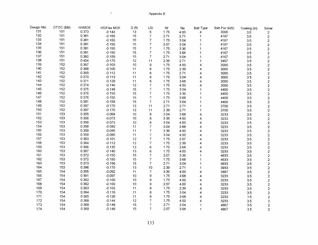
Appendix B
Design Nbr. DTOC ($M) HAMOE HD/Flex MOE D (ft) L/D Nf Na Batt Type Batt Pwr (kW) Coating (in) Sonar131 151 0.373 -0 143 13 6 1 75 400 4 3000 3.5 2132 151 0.381 -0 150 15 7 271 2.71 1 4167 3.5 2133 151 0.381 -0 150 15 7 1 75 304 1 4167 3.5 2134 151 0 381 -0 150 15 7 2 07 3 04 1 4167 3.5 2135 151 0 381 -0 150 15 7 1 75 3 36 1 4167 35 2136 151 0.381 -0 150 15 7 1 75 368 1 4167 35 2137 151 0.382 -0.159 15 7 2.71 3.04 1 4167 3.5 2138 151 0 404 -0 170 12 11 2.39 2 71 1 3467 35 2139 152 0.367 -0 103 10 9 1.75 400 4 3000 3.5 2140 152 0 368 -0.105 11 8 1 75 2 39 4 3000 3.5 2141 152 0.369 -0 112 11 8 1 75 271 4 3000 3.5 2142 152 0.370 -0 119 11 8 1 75 3.04 4 3000 35 2143 152 0 371 -0 129 11 8 1 75 3 68 4 3000 3.5 2144 152 0 374 -0.146 12 7 1 75 4 00 4 3000 3.5 2145 152 0 375 -0.148 15 7 1 75 3 04 1 4400 3.5 2146 152 0 376 -0 150 15 7 1 75 3 36 1 4400 3.5 2147 152 0 376 -0 150 15 7 1 75 3 68 1 4400 3.5 2148 152 0.381 -0.159 15 7 271 304 1 4400 3.5 2149 152 0 397 -0 170 12 11 2.71 2.71 1 3700 35 2150 152 0.397 -0 170 12 11 239 2.71 1 3700 3.5 2151 153 0 355 -0.068 10 8 3 04 3 68 4 3233 3.5 2152 153 0 356 -0.073 10 8 3 36 4 00 4 3233 35 2153 153 0 356 -0 073 10 8 3 04 4 00 4 3233 35 2154 153 0.358 -0 090 11 7 3.04 3 68 4 3233 3.5 2155 153 0.359 -0.095 11 7 336 400 4 3233 35 2156 153 0 359 -0.095 11 7 3 04 4.00 4 3233 35 2157 153 0 363 -0.101 12 7 1 75 2 07 4 3233 3.5 2158 153 0.364 -0.112 12 7 1 75 239 4 3233 3.5 2159 153 0 366 -0.135 13 6 1 75 3.68 4 3233 3.5 2160 153 0.367 -0 140 13 6 1 75 400 4 3233 3.5 2161 153 0.372 -0 150 15 7 2.07 3.36 1 4633 3.5 2162 153 0 372 -0.150 15 7 1.75 3 68 1 4633 3.5 2163 153 0.373 -0.156 15 7 2.71 3.04 1 4633 3.5 2164 153 0.396 -0.170 13 10 2.39 2.71 1 3933 35 2165 154 0.355 -0.092 11 7 3.36 4.00 4 3467 3.5 2166 154 0 361 -0.097 10 9 1.75 3.68 4 3233 3.5 2167 154 0.362 -0.100 10 9 1.75 400 4 3233 3.5 2168 154 0 362 -0.100 10 9 2.07 4.00 4 3233 3.5 2169 154 0.363 -0102 11 8 1.75 2.39 4 3233 3.5 2170 154 0.364 -0.116 11 8 1 75 304 4 3233 3.5 2171 154 0 365 -0.126 11 8 1.75 3 68 4 3233 3.5 2172 154 0 368 -0.144 12 7 1.75 4 00 4 3233 35 2173 154 0 369 -0.149 15 7 2 71 3 04 1 4867 35 2174 154 0 369 -0 149 15 7 2.07 3 68 1 4867 35 2
133
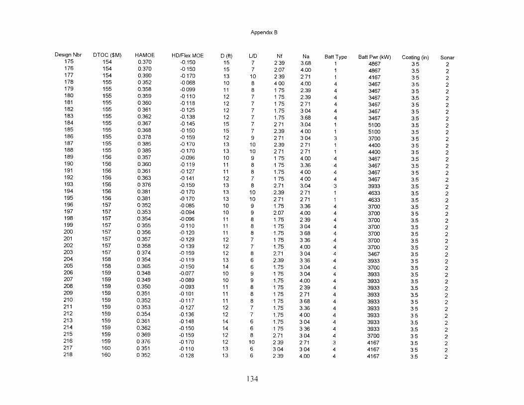
Appendix B
Design Nbr175176177178179180181182183184185186187188189190191192193194195196197198199200201202203204205206207208209210211212213214215216217218
DTOC ($M)154154154155155155155155155155155155155155156156156156156156156157157157157157157157157158158159159159159159159159159159159159160160
HAMOE0.3700.3700.3900 3520.3580.3590 3600 3610.3620.3670.3680.3780 3850 3850.3570.3600.3610.3630 3760.3810.3810 3520.3530.3540 3550 3560.3570.3580 3740 3540.3650.3480.3490.3500.3510.3520 3530.3540.3610.3620 3690 3760 3510 352
HD/Flex MOE-0.150-0 150-0 170-0 068-0 099-0 110-0 118-0 125-0.138-0 145-0 150-0 159-0 170-0 170-0.096-0 119-0 127-0 141-0.159-0 170-0 170-0 085-0.094-0 096-0 110-0 120-0 129-0 139-0 159-0 119-0 150-0.077-0 089-0 093-0 101-0 117-0 127-0.136-0 148-0 150-0 159-0 170-0 110-0 128
D (ft)1515131011121212121515121313101111121313131010111111121212131410101111111212141412121313
Nf2 392.072 394 001 751 751 751.751.752712.392712.392711 751 751.751 752.712.392711.752.071.751 751.751 751.752.712.391.751 751.751 751 751 751.751.751.751 752.712 393 042 39
Na3.684.002714.002.392.392713 043.683.044 003 042712714.003.364 004 003.042712713.364.002 393 043 683 364.003 043 363.043 044.002392713 683.364003 043 363 042713044.00
Batt Type11144444411311444431144444444444444444444344
Batt Pwr (kW)48674867416734673467346734673467346751005100370044004400346734673467346739334633463337003700370037003700370037003467393337003933393339333933393339333933393339333700416741674167
Coating (in)353.53535353.535353.53.53.53535353.53.5353.53.53.53.53.5353.53.53.53.53.53.5353.53.53.53.53.53535353.53.5353.5353.5
Sonar22222222222222222222222222222222222222222222
134
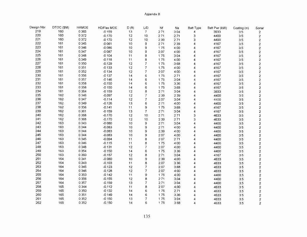
Appendix B
Design Nbr DTOC ($M) HAMOE HD/Flex MOE219 160 0 365 -0 159220 160 0 372 -0.170221 160 0 372 -0170222 161 0 345 -0 061223 161 0 346 -0 086224 161 0.347 -0 087225 161 0 348 -0104226 161 0.349 -0.118227 161 0 350 -0.129228 161 0 351 -0 133229 161 0 352 -0 134230 161 0 356 -0137231 161 0 357 -0 146232 161 0.358 -0.150233 161 0 358 -0 150234 161 0364 -0159235 162 0 346 -0.097236 162 0 347 -0.114237 162 0 349 -0.126238 162 0 356 -0.141239 162 0.361 -0159240 162 0 368 -0.170241 162 0 368 -0.170242 163 0 343 -0 080243 163 0.344 -0.083244 163 0 344 -0.083245 163 0 344 -0.083246 163 0.345 -0.094247 163 0 346 -0.115248 163 0 348 -0131249 163 0 354 -0 150250 163 0 360 -0.157251 164 0 341 -0 080252 164 0.343 -0.103253 164 0 345 -0.123254 164 0 346 -0.128255 164 0 353 -0 142256 164 0 356 -0.155257 164 0 357 -0.159258 165 0 344 -0.112259 165 0 350 -0132260 165 0 351 -0149261 165 0 352 -0150262 165 0 352 -0.150
D (ft)1312121010101111121212141414141212121311131212101010101111121412101112121112131114141314
Nf271
2712 392711 752.071 751 751 751.752 071 751 751 751 752712 392.072711 752712 712 392712712.392 072071 752 071 752712 392.072.072 071 752712.712 071 751 751 751 75
Na3 042.712712 394004003044.003 684 004002713043.363.683042 393.044.003.683042712713.044004 004.002714004.003 363.044.003 363.684004 003.043044.002.713.363 043 68
Batt Type Batt Pwr (kW)4 39333 44003 44004 41674 41674 41674 41674 41674 41674 41674 41674 41674 41674 41674 41674 39334 44004 44004 44004 41674 41673 46333 46334 44004 44004 44004 44004 44004 44004 44004 44004 41674 46334 46334 46334 46334 44004 44004 44004 46334 46334 46334 46334 4633
135
Coating (in)3535353.53.535353535353.53.53.535353535353535353.53.53.5353535353.53.535353.53.5353.53.53.53.5353.5353.53.5
Sonar22222222222222222222222222222222222222222222
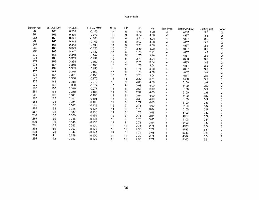
Appendix B
Design Nbr DTOC ($M) HAMOE HDIFlex MOE D (ft) L/D Nf Na Batt Type Batt Pwr (kW) Coating (in) Sonar263 165 0.352 -0.150 14 6 1 75 400 4 4633 35 2264 166 0.339 -0 076 10 9 3 04 4.00 4 4867 35 2265 166 0.341 -0 105 11 8 271 3.04 4 4867 35 2266 166 0.342 -0 109 11 8 207 4.00 4 4867 35 2267 166 0.342 -0 109 11 8 2.71 4.00 4 4867 35 2268 166 0 343 -0.125 12 7 2 39 4.00 4 4867 3.5 2269 166 0 347 -0 130 14 6 1 75 2 71 4 4867 35 2270 166 0 348 -0 147 14 6 1 75 3.36 4 4867 3.5 2271 166 0.353 -0 153 12 8 271 3.04 4 4633 35 2272 166 0.354 -0 159 13 7 271 3.04 4 4633 3.5 2273 167 0 349 -0 150 13 7 1 75 3.04 4 4867 3.5 2274 167 0 349 -0.150 14 6 1 75 3 68 4 4867 35 2275 167 0.349 -0 150 14 6 1 75 400 4 4867 35 2276 167 0.351 -0 158 13 7 271 3.04 4 4867 35 2277 167 0 366 -0.170 11 11 2 39 2.71 4 4400 35 2278 168 0 338 -0 072 10 9 4 00 4 00 4 5100 3.5 2279 168 0.338 -0 072 10 9 3 68 4 00 4 5100 35 2280 168 0.339 -0.077 11 8 368 2.39 4 5100 3.5 2281 168 0.340 -0 105 11 8 239 4.00 4 5100 35 2282 168 0 341 -0 106 11 8 3 04 4.00 4 5100 3.5 2283 168 0 341 -0 106 11 8 3 36 4.00 4 5100 3.5 2284 168 0 341 -0 106 11 8 2.71 4.00 4 5100 35 2285 168 0 342 -0.122 12 7 2 71 4.00 4 5100 35 2286 168 0 346 -0 137 14 6 1.75 3.04 4 5100 35 2287 168 0 347 -0 150 14 6 1 75 3 68 4 5100 3.5 2288 168 0 350 -0 151 12 8 2 71 3.04 4 4867 35 2289 169 0 345 -0 131 11 9 1.75 3.68 4 5100 35 2290 169 0 349 -0 156 13 7 2.71 3.04 4 5100 3.5 2291 169 0 363 -0 170 11 11 2 71 2 71 4 4633 3.5 2292 169 0 363 -0 170 11 11 2 39 2.71 4 4633 3.5 2293 170 0.347 -0.149 14 6 1 75 368 4 5333 35 2294 171 0.359 -0 170 11 11 239 2.71 4 4867 3.5 2295 172 0 357 -0 170 11 11 2.39 2.71 4 5100 3.5 2
136
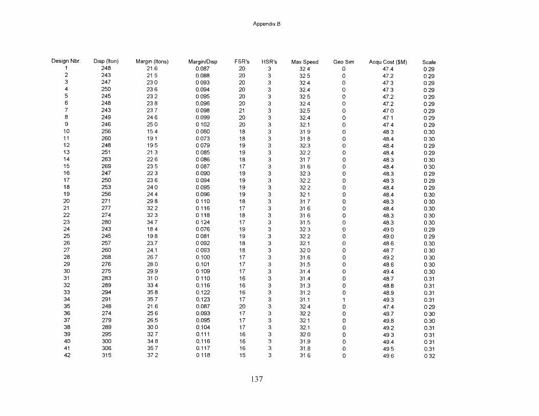
Appendix B
Design Nbr. Disp (Iton) Margin (Itons) Margin/Disp FSR's HSR's Max Speed Geo Sim Acqu Cost ($M) Scale1 248 21.6 0.087 20 3 32 4 0 47.4 0 292 243 21 5 0.088 20 3 325 0 47.2 0293 247 230 0093 20 3 324 0 473 0294 250 236 0.094 20 3 32.4 0 473 0295 245 232 0095 20 3 325 0 47.2 0296 248 23 8 0.096 20 3 32 4 0 47.2 0 297 243 23 7 0 098 21 3 32.5 0 47 0 0 298 249 246 0.099 20 3 32.4 0 471 0299 246 250 0102 20 3 32.1 0 474 02910 256 154 0 060 18 3 31 9 0 48 3 0.3011 260 191 0 073 18 3 31 8 0 48.4 0 3012 248 195 0 079 19 3 32.3 0 48.4 0 2913 251 21 3 0085 19 3 322 0 48.4 02914 263 226 0086 18 3 31 7 0 483 03015 269 235 0087 17 3 31 6 0 48.4 03016 247 223 0090 19 3 323 0 48.3 02917 250 236 0094 19 3 322 0 483 02918 253 24 0 0 095 19 3 32 2 0 48.4 0 2919 256 24 4 0.096 19 3 32 1 0 48.4 0.3020 271 298 0110 18 3 31 7 0 48.3 03021 277 32 2 0116 17 3 31 6 0 48.4 0.3022 274 32 3 0118 18 3 31 6 0 48.3 0 3023 280 34 7 0124 17 3 31.5 0 48.3 0 3024 243 184 0 076 19 3 32 3 0 49 0 0.2925 245 198 0081 19 3 322 0 49.0 02926 257 23.7 0 092 18 3 32.1 0 48 6 0.3027 260 24.1 0093 18 3 320 0 487 03028 268 26 7 0.100 17 3 31.6 0 49.2 0 3029 276 28 0 0.101 17 3 31.5 0 48 6 0 3030 275 29.9 0109 17 3 31.4 0 49.4 0.3031 283 31 0 0110 16 3 31.4 0 48.7 0.3132 289 33 4 0.116 16 3 31.3 0 48.8 0.3133 294 35 8 0.122 16 3 31.2 0 48.9 0.3134 291 35 7 0.123 17 3 31.1 1 49.3 0.3135 248 21.6 0.087 20 3 32 4 0 47.4 0 2936 274 25 6 0.093 17 3 32 2 0 49.7 0 3037 279 26.5 0.095 17 3 32 1 0 49.8 0.3038 289 30 0 0.104 17 3 32.1 0 49.2 0.3139 295 32 7 0.111 16 3 32 0 0 49 3 0 3140 300 34 8 0.116 16 3 31.9 0 49.4 0 3141 306 35 7 0.117 16 3 31.8 0 49 5 0.3142 315 372 0118 15 3 31 6 0 496 032
137
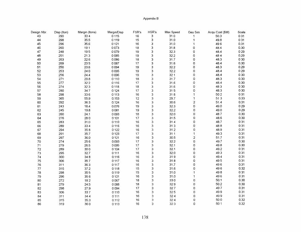
Appendix B
Design Nbr. Disp (Iton) Margin (Itons) Margin/Disp FSR's HSR's Max Speed Geo Sim Acqu Cost ($M) Scale43 290 33 4 0115 16 3 31 0 1 50.3 0 3144 298 35.5 0119 15 3 31.0 1 49.8 0 3145 296 35.6 0121 16 3 31.0 1 49 6 0.3146 260 191 0 073 18 3 31.8 0 48.4 0.3047 248 195 0079 19 3 32.3 0 48.4 02948 251 21.3 0 085 19 3 32.2 0 48 4 0.2949 263 22.6 0.086 18 3 31.7 0 48.3 0 3050 269 23 5 0 087 17 3 31.6 0 48.4 0.3051 250 23.6 0 094 19 3 32.2 0 48.3 0.2952 253 24 0 0 095 19 3 32.2 0 48.4 0 2953 256 24.4 0 096 19 3 32 1 0 48.4 0 3054 271 29.8 0110 18 3 31.7 0 48.3 0.3055 277 32 2 0116 17 3 31.6 0 48.4 0.3056 274 323 0118 18 3 31.6 0 483 03057 280 347 0124 17 3 31 5 0 48.3 03058 298 336 0113 16 3 31 8 1 502 03159 365 55.9 0.153 12 3 29.7 1 51 3 0.3360 292 36 3 0.124 16 3 30.6 2 51.4 0.3161 243 18.4 0.076 19 3 32.3 0 49.0 0 2962 245 19.8 0 081 19 3 32.2 0 49.0 0 2963 260 24.1 0 093 18 3 32.0 0 48 7 0.3064 276 28 0 0101 17 3 31.5 0 48.6 0.3065 283 31.0 0110 16 3 31 4 0 48.7 0 3166 289 33 4 0116 16 3 31 3 0 48 8 0 3167 294 35 8 0122 16 3 31 2 0 48.9 0.3168 291 35.7 0123 17 3 31 1 1 49.3 0.3169 297 36.0 0121 16 3 30.5 2 51.7 0.3170 274 25 6 0.093 17 3 32.2 0 49.7 0.3071 279 26.5 0 095 17 3 32.1 0 49.8 0.3072 289 30 0 0104 17 3 32.1 0 49.2 0 3173 295 32.7 0111 16 3 32.0 0 49 3 0 3174 300 34 8 0.116 16 3 31 9 0 49.4 0.3175 306 357 0117 16 3 31 8 0 495 0.3176 311 36 3 0117 16 3 31.7 0 49 6 0.3177 315 37.2 0118 15 3 31.6 0 49 6 0.3278 298 35 5 0.119 15 3 31.0 1 49 8 0 3179 296 35 6 0121 16 3 31.0 1 49 6 0 3180 272 182 0 067 18 3 33 0 0 50.1 0.3081 279 24.5 0 088 18 3 32 9 0 50.2 0.3082 298 27.9 0 094 17 3 32 7 0 49 7 0.3183 306 337 0110 16 3 325 0 499 03184 311 34 4 0111 16 3 32 4 0 49 9 0.3185 315 35.3 0.112 16 3 32 4 0 50 0 0.3286 319 360 0113 16 3 323 0 501 0.32
138

Appendix B
Design Nbr Disp (Iton) Margin (Itons) Margin/Disp FSR's HSR's Max Speed Geo Sim Acqu Cost ($M) Scale87 287 33.2 0116 17 3 32 0 0 49 9 0.3188 292 35.4 0121 16 3 31.9 0 50 0 0.3189 298 33 6 0113 16 3 31 8 1 50.2 0.3190 365 55 9 0 153 12 3 29.7 1 51 3 0 3391 292 36 3 0.124 16 3 30 6 2 51.4 0 3192 305 27 0 0.088 17 3 33 2 0 50.2 0 3193 312 29 7 0 095 17 3 33 1 0 50 3 0 3294 308 29 4 0 095 17 3 33.2 0 50.3 0.3195 319 34.1 0.107 16 3 33 0 0 50.4 0.3296 292 33.2 0114 17 3 32 7 0 50 4 0.3197 296 35 0 0118 17 3 32.6 0 50 5 0.3198 303 36 6 0121 17 3 32 5 0 50.6 0.3199 365 54 2 0148 13 3 30 4 1 51 7 0.33100 300 36 3 0121 15 3 30.4 2 51.8 0.31101 297 36.0 0121 16 3 30 5 2 51 7 0 31102 298 29 6 0 099 17 3 33 2 1 50 9 0 31103 304 33 4 0110 17 3 33 1 0 51 0 0 31104 308 35.2 0114 17 3 331 0 51.1 0.31105 317 36 8 0116 16 3 32.9 0 51.2 0.32106 323 37 8 0117 16 3 32.8 0 51.3 0.32107 365 52 4 0 143 14 3 31 1 1 52.1 0.33108 295 27 0 0 092 18 4 33 9 0 51 9 0 31109 298 29 6 0 099 18 4 33 8 0 51 9 0.31110 326 36.2 0111 16 3 33 4 0 51 8 0.32111 365 50 6 0138 14 3 31 8 1 52 5 0 33112 345 47 6 0138 13 2 29 4 2 53 8 0.33113 342 47.3 0138 13 2 29 4 2 53 8 0 33114 386 61 5 0159 11 2 28.8 2 54 2 0 34115 382 61.2 0160 11 2 28 9 2 54.1 0.34116 305 27.6 0 090 18 4 34 3 0 52.4 0.31117 320 33.0 0103 17 4 34.2 0 52.0 0.32118 326 34.1 0105 17 4 34.1 0 52.1 0.32119 337 41.3 0123 16 3 32 9 0 52.3 0.32120 365 48.7 0133 15 3 32.5 1 52.8 0.33121 345 45.7 0.133 13 3 30 1 2 54.2 0 33122 342 45 4 0133 13 3 30 2 2 54 2 0.33123 136 4.3 0 032 66 4 36.5 0 48.2 0.24124 140 6.5 0 047 64 4 36.3 0 48.3 0.24125 138 6.5 0.047 65 4 36 4 0 48 3 0.24126 149 7.8 0 052 60 4 36 0 0 48.1 0.25127 152 10.5 0069 59 4 359 0 48.2 025128 171 142 0 083 52 4 34.8 0 48.4 0.26129 176 164 0093 50 4 347 0 48.5 026130 184 198 0107 48 4 34 4 0 48 7 0.26
139
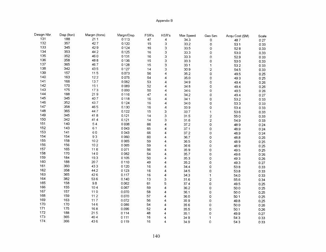
Appendix B
Design Nbr. Disp (Iton) Margin (Itons) Margin/Disp FSR's HSR's Max Speed Geo Sim Acqu Cost ($M) Scale131 188 21 1 0113 47 4 34.3 0 48 7 0 27132 357 42 7 0.120 15 3 33.2 0 53 1 0 33133 345 42 9 0 124 16 3 33.5 0 52 8 0.33134 353 44 2 0.125 16 3 33.3 0 53.0 0.33135 352 46 0 0131 16 3 33 3 0 52.9 0 33136 358 48 8 0 136 15 3 33 3 0 53 0 0.33137 365 46 7 0128 15 3 33 1 1 53 2 0 33138 342 43 5 0127 14 3 30 9 2 54.5 0.33139 157 11 5 0.073 56 4 35.2 0 49.5 0.25140 163 122 0 075 54 4 35.0 0 49 3 0 25141 166 137 0.082 53 4 34 9 0 49.4 0.26142 170 151 0 089 52 4 34 8 0 49.4 0.26143 175 173 0 099 50 4 34 6 0 49.5 0 26144 188 21 9 0116 47 4 34.2 0 49.4 0 27145 345 40 7 0118 16 4 34 1 0 53.2 0 33146 352 43 7 0124 16 4 34 0 0 53 3 0 33147 358 46 5 0.130 16 4 33 9 0 53 4 0 33148 365 44 7 0.122 15 3 33 7 1 53 6 0.33149 345 41 8 0.121 14 3 31.5 2 55 0 0.33150 342 41 4 0.121 14 3 31.6 2 54.9 0 33151 140 54 0 038 66 4 37.2 0 48 9 0 24152 143 61 0 043 65 4 37.1 0 48.9 0 24153 141 60 0 043 66 4 37.2 0 48.9 0 24154 154 93 0 060 60 4 36.7 0 48.8 0.25155 158 102 0 065 59 4 36.5 0 48 9 0 25156 156 102 0 065 59 4 36 6 0 48 9 0 25157 165 116 0 071 56 4 35 9 0 49.5 0 25158 170 140 0 082 54 4 35.7 0 49.6 0 26159 184 19.3 0105 50 4 35.3 0 49 3 0.26160 188 20 7 0110 49 4 35.2 0 49.3 0 27161 360 43 3 0120 16 4 34.4 0 53 8 0.33162 358 44.2 0123 16 4 34 5 0 53.8 0 33163 365 42 6 0.117 16 4 34.3 1 54.0 0 33164 382 53 6 0.140 13 3 31.6 2 55.6 0.34165 158 9.8 0.062 61 5 37 4 0 49.5 0.25166 155 104 0.067 59 4 36.2 0 50 0 0 25167 157 11 0 0.070 58 4 36.1 0 50 0 0.25168 159 11 2 0.070 57 4 36.0 0 50 1 0 25169 163 11 7 0.072 56 4 35 9 0 49.8 0.25170 170 146 0 086 54 4 35 6 0 50 0 0 26171 175 168 0.096 52 4 35.5 0 50.1 0.26172 188 21 5 0114 48 4 35.1 0 49.9 0.27173 365 40 4 0111 16 4 34 9 1 54 3 0 33174 366 43 6 0119 16 4 34.9 0 54 3 0 33
140
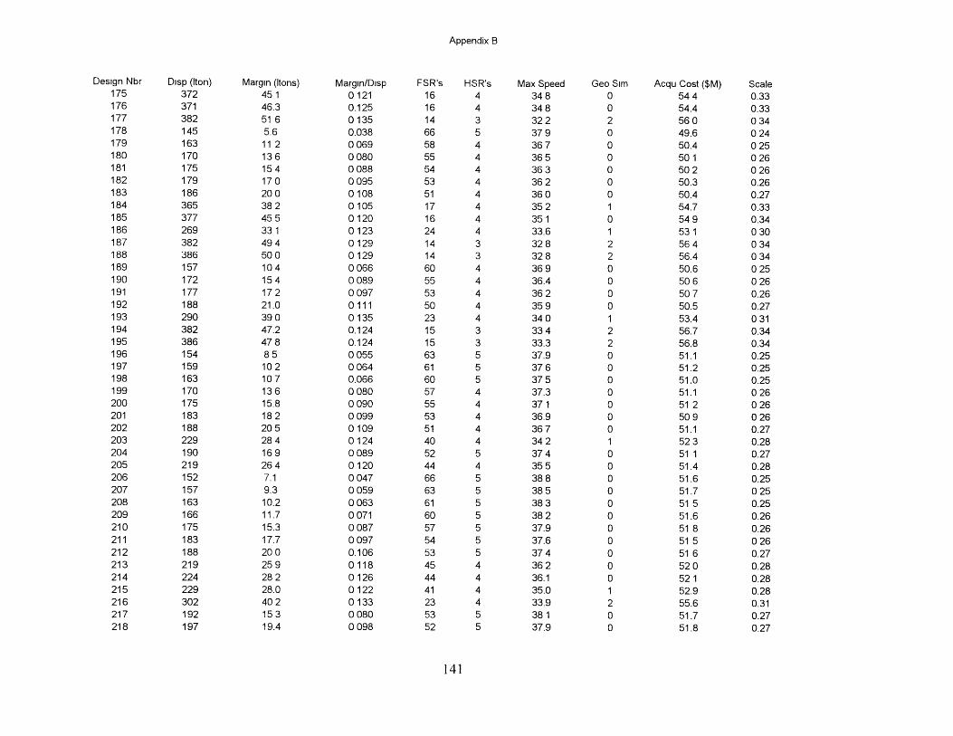
Appendix B
Design Nbr Disp (Iton) Margin (Itons) Margin/Disp FSR's HSR's Max Speed Geo Sim Acqu Cost ($M) Scale175 372 45 1 0121 16 4 34 8 0 54 4 0.33176 371 46.3 0.125 16 4 34 8 0 54.4 0.33177 382 51 6 0 135 14 3 32 2 2 56 0 0 34178 145 5.6 0.038 66 5 37 9 0 49.6 0 24179 163 11 2 0 069 58 4 36 7 0 50.4 0 25180 170 136 0 080 55 4 36 5 0 50 1 0 26181 175 154 0088 54 4 363 0 502 026182 179 170 0 095 53 4 36 2 0 50.3 0.26183 186 20 0 0108 51 4 36 0 0 50.4 0.27184 365 38 2 0105 17 4 35 2 1 54.7 0.33185 377 455 0120 16 4 351 0 549 0.34186 269 33 1 0123 24 4 33.6 1 53 1 0 30187 382 494 0129 14 3 328 2 564 034188 386 500 0129 14 3 328 2 56.4 034189 157 104 0 066 60 4 36 9 0 50.6 0 25190 172 154 0 089 55 4 36.4 0 50 6 0 26191 177 172 0 097 53 4 36 2 0 50 7 0.26192 188 21.0 0111 50 4 35 9 0 50.5 0.27193 290 390 0135 23 4 340 1 53.4 031194 382 47.2 0.124 15 3 33 4 2 56.7 0.34195 386 47 8 0.124 15 3 33.3 2 56.8 0.34196 154 85 0 055 63 5 37.9 0 51.1 0.25197 159 102 0 064 61 5 37 6 0 51.2 0.25198 163 107 0.066 60 5 37 5 0 51.0 0.25199 170 136 0 080 57 4 37.3 0 51.1 0 26200 175 15.8 0 090 55 4 37 1 0 51 2 0 26201 183 182 0 099 53 4 36.9 0 50 9 0 26202 188 205 0109 51 4 367 0 51.1 0.27203 229 28 4 0 124 40 4 34 2 1 52 3 0.28204 190 169 0 089 52 5 37 4 0 51 1 0.27205 219 26 4 0 120 44 4 35 5 0 51.4 0.28206 152 7.1 0 047 66 5 38 8 0 51.6 0.25207 157 9.3 0 059 63 5 38 5 0 51.7 0 25208 163 10.2 0 063 61 5 38 3 0 51 5 0.25209 166 11.7 0 071 60 5 38 2 0 51.6 0.26210 175 15.3 0 087 57 5 37.9 0 51 8 0.26211 183 17.7 0 097 54 5 37.6 0 51 5 0 26212 188 20 0 0.106 53 5 37 4 0 51 6 0.27213 219 25 9 0118 45 4 36 2 0 52 0 0.28214 224 28 2 0 126 44 4 36.1 0 52 1 0.28215 229 28.0 0 122 41 4 35.0 1 52.9 0.28216 302 40 2 0 133 23 4 33.9 2 55.6 0.31217 192 153 0 080 53 5 38 1 0 51.7 0.27218 197 19.4 0 098 52 5 37.9 0 51.8 0.27
141
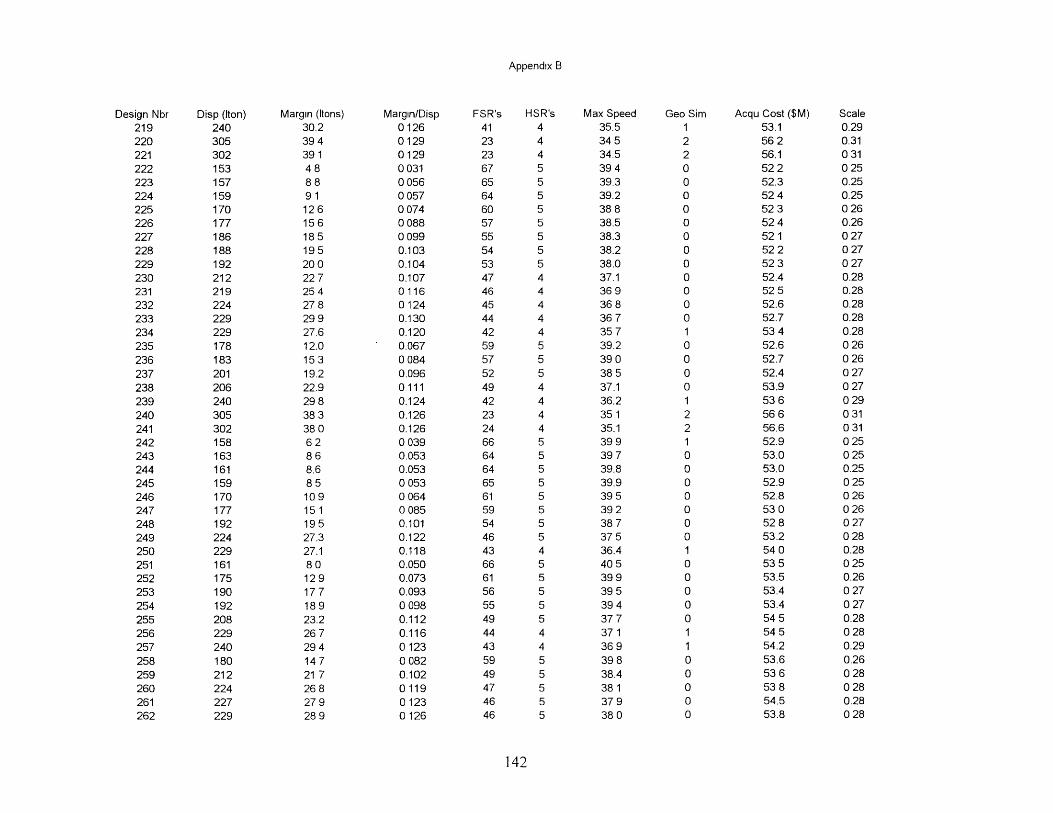
Appendix B
Design Nbr Disp (Iton) Margin (Itons) Margin/Disp FSR's HSR's Max Speed Geo Sim Acqu Cost ($M) Scale219 240 30.2 0126 41 4 35.5 1 53.1 0.29220 305 39 4 0129 23 4 34 5 2 56 2 0.31221 302 39 1 0 129 23 4 34.5 2 56.1 0 31222 153 48 0031 67 5 394 0 522 025223 157 88 0 056 65 5 39.3 0 52.3 0.25224 159 91 0 057 64 5 39.2 0 52 4 0.25225 170 126 0074 60 5 388 0 523 026226 177 156 0 088 57 5 38.5 0 52 4 0.26227 186 185 0099 55 5 38.3 0 521 027228 188 195 0.103 54 5 38.2 0 52 2 0 27229 192 20 0 0.104 53 5 38.0 0 52 3 0 27230 212 22 7 0.107 47 4 37.1 0 52.4 0.28231 219 25 4 0116 46 4 36 9 0 52 5 0.28232 224 27 8 0 124 45 4 36 8 0 52.6 0.28233 229 29 9 0.130 44 4 36 7 0 52.7 0.28234 229 27.6 0.120 42 4 35 7 1 53 4 0.28235 178 12.0 0.067 59 5 39.2 0 52.6 0 26
236 183 153 0084 57 5 390 0 52.7 026237 201 19.2 0.096 52 5 38 5 0 52.4 0 27
238 206 22.9 0111 49 4 37.1 0 53.9 0 27239 240 29 8 0.124 42 4 36.2 1 53 6 0 29
240 305 38 3 0.126 23 4 35 1 2 56 6 0 31241 302 38 0 0.126 24 4 35.1 2 56.6 0 31
242 158 62 0039 66 5 399 1 52.9 025243 163 86 0.053 64 5 397 0 53.0 025244 161 8.6 0.053 64 5 39.8 0 53.0 0.25245 159 85 0 053 65 5 39.9 0 52.9 0 25246 170 109 0064 61 5 395 0 52.8 026247 177 151 0085 59 5 392 0 530 026248 192 195 0.101 54 5 387 0 528 027249 224 27.3 0.122 46 5 37 5 0 53.2 0 28
250 229 27.1 0.118 43 4 36.4 1 54 0 0.28251 161 80 0.050 66 5 405 0 535 025252 175 129 0.073 61 5 39 9 0 53.5 0.26253 190 177 0.093 56 5 395 0 53.4 027254 192 189 0098 55 5 394 0 53.4 027255 208 23.2 0.112 49 5 37 7 0 54 5 0.28256 229 26 7 0.116 44 4 37 1 1 54 5 0 28
257 240 29 4 0 123 43 4 36 9 1 54.2 0.29258 180 147 0082 59 5 398 0 53.6 0.26259 212 21 7 0.102 49 5 38.4 0 53 6 0 28
260 224 26 8 0119 47 5 38 1 0 53 8 0 28
261 227 279 0123 46 5 379 0 54.5 0.28262 229 289 0126 46 5 380 0 53.8 028
142
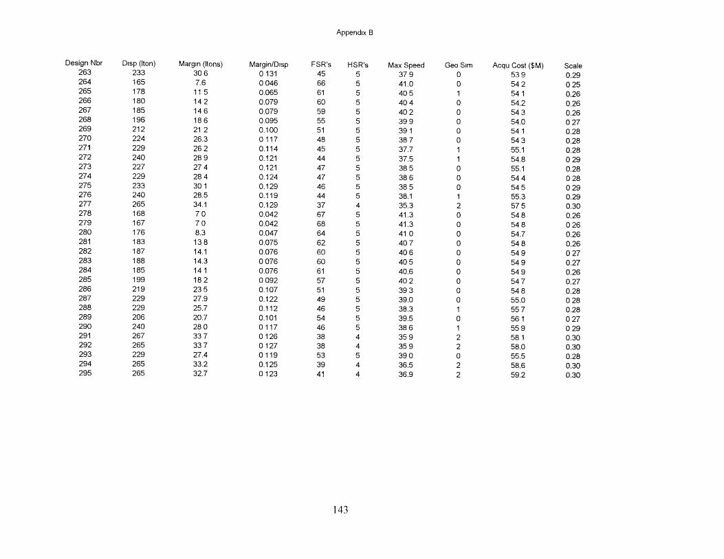
Appendix B
Design Nbr Disp (Iton) Margin (Itons) Margin/Disp FSR's HSR's Max Speed Geo Sim Acqu Cost ($M) Scale263 233 30 6 0131 45 5 37 9 0 53 9 0.29264 165 7.6 0 046 66 5 41.0 0 54 2 0 25265 178 11 5 0.065 61 5 40 5 1 54 1 0.26266 180 142 0.079 60 5 40 4 0 54.2 0.26267 185 146 0.079 59 5 40 2 0 54 3 0.26268 196 186 0.095 55 5 39 9 0 54.0 0 27269 212 21 2 0.100 51 5 391 0 541 0.28270 224 26.3 0117 48 5 38 7 0 54 3 0.28271 229 26 2 0.114 45 5 37.7 1 55.1 0.28272 240 28 9 0.121 44 5 37.5 1 54.8 0 29273 227 27 4 0.121 47 5 38 5 0 55.1 0.28274 229 28 4 0.124 47 5 38 6 0 54 4 0 28275 233 30 1 0.129 46 5 38 5 0 54 5 0 29276 240 28.5 0.119 44 5 38.1 1 55.3 0.29277 265 34.1 0.129 37 4 35.3 2 57 5 0.30278 168 70 0.042 67 5 41.3 0 54 8 0.26279 167 70 0.042 68 5 41.3 0 54 8 0 26280 176 8.3 0.047 64 5 41 0 0 54.7 0.26281 183 138 0.075 62 5 40 7 0 54 8 0.26282 187 14.1 0.076 60 5 40 6 0 54 9 0 27283 188 14.3 0 076 60 5 40 5 0 54 9 0.27284 185 141 0.076 61 5 40.6 0 54 9 0.26285 199 182 0 092 57 5 40 2 0 54 7 0.27286 219 23 5 0.107 51 5 39 3 0 54 8 0.28287 229 27.9 0.122 49 5 39.0 0 55.0 0 28288 229 25.7 0.112 46 5 38.3 1 55 7 0.28289 206 20.7 0.101 54 5 39.5 0 56 1 0 27290 240 28 0 0117 46 5 38 6 1 55 9 0 29291 267 33 7 0126 38 4 35 9 2 58 1 0.30292 265 33 7 0 127 38 4 35 9 2 58.0 0.30293 229 27.4 0119 53 5 39 0 0 55.5 0.28294 265 33.2 0.125 39 4 36.5 2 58.6 0.30295 265 32.7 0 123 41 4 36.9 2 59.2 0.30
143

(This page intentionally blank.)
144
Appendix C
PROGRAM MAINC************************ *** ***w************* * *
C This is the main program for Multi-Objective Evolutionary Program (EP)
C for Large Scale Vehicle II.CC Programmer: Allan Andrew 5/5/98
C *** ****** **************** *****************************************
IMPLICIT NONE
INCLUDE 'VARIABLES.F'
C Open file for base-10 population characteristics after last generation.
OPEN (UNIT=21, FILE='POPLN2.OUT', STATUS='NEW')
C Open file for binary population characteristics after last generation.
OPEN (UNIT=22, FILE='BIPOP2.OUT', STATUS='NEW')C Open file for base-10 population characteristics for restart.
C OPEN (UNIT=30, FILE='POPLN3.OUT', STATUS='OLD')C Open file for count of number of non-dominated designs.
OPEN (UNIT=32, FILE='NUM ND.OUT', STATUS='NEW')C Open file for characteristics of non-dominated designs found.
OPEN (UNIT=41, FILE='NON DOM2.OUT', STATUS='NEW')C Open file for characteristics of non-dominated designs previously found.
OPEN (UNIT=51, FILE='NON DOM3.OUT', STATUS='OLD')
C Open file of non-dominated designs previously found using exhaustive
search.OPEN (UNIT=71, FILE='EXH SEARCH.OUT', STATUS='OLD')
C Open file to record number of non-dominated designs found in EP search
that were also found in exhaustive search.OPEN (UNIT=72, FILE='NBR FOUND.OUT', STATUS='NEW')
C Open file to mark start time.OPEN (UNIT=80, FILE='STARTTIME.OUT', STATUS='NEW')
READ (71,*) EXH SEARCH NUM
DO I=l, 326READ (71, 7040) (EXHSEARCH(J, I), J=1,3)
END DO
C Generate the RANG array by assigning parameter values to the array.
CALL RNGGEN (DMIN,DMAX,LDMIN,LDMAX,NFMIN,NFMAX,NAMIN,NAMAX,* BTMIN,BTMAX,BPMIN,BPMAX,COTMIN,COTMAX,SONMIN,SONMAX,* DNUM,LDNUM,NFNUM,NANUM,BTNUM,BPNUM,COTNUM,SONNUM,* VARNUM, RANG)
C USEOLD NON DOM =.TRUE. forces program to begin from a previouslyC defined non-dominated array.
USEOLD NON DOM = .true.
IF (USEOLD NON DOM) THENREAD (51, *) NUM NON DOM
c PRINT *, 'NUM-NON DOM = ', NUM NON DOMDO I=l, NUM NON DOM
READ (51, 7020) (NON DOM (J,I),J=1,NUM POP CHAR)END DO
ELSENUM NON DOM = 0
END IF
C Set the following line to restart the EP more than once.
DO 4000 RUN NUM=1, 1
145
Appendix C
C USEOLD POPLN=.TRUE. forces program to begin from a previously definedC generation. Otherwise the population is selected randomly.
USEOLD POPLN=.FALSE.
GEN NUM = 1ADD TNUM = 0REMOVE TNUM = 0
C Generate a random populationDO 220 I=1, GENSIZ
DO 200 J=l, GENELX = ran2(IDUM)GENE(J) = NINT(X)
200 CONTINUE
C Translate the gene from binary to base 10.CALL DECODE (GENE, GENEL, RANG, VARNUM, MBR)
C Balance the individual member to ensure a feasible design.CALL BALANCE (MBR, BALANCE OUT, WCOST)
C Calculate the Measures of Performance (MOPs)CALL CALC MOPS (MBR, BALANCE OUT,
FR SPD RUNS, HI SPD RUNS, VMAX,VMAX HA, SCALE)
C Calculate discounted total ownership cost and acquisition cost.CALL COST (MBR, WCOST, BALANCE OUT, DTOC, ACQU COST)
C Calculate the Measures of EffectivenessCALL CALC HA MOE (VMAX HA, HI SPD RUNS, MBR,
HAMOE)CALL CALC HD MOE (MBR, BALANCEOUT, FR SPD RUNS,
HDMOE, GEO)
C Assign characteristics and output of BALANCE, CALC MOPSC COST, HDMOE and HAMOE to the population array.C HDMOE is made negative so that all comparisons are made withC lower values preferred.
CALL REPLACE (EBIPOP, GENE, GENEL, PCPLN, NUM POP CHAR,GENSIZ, I, DTOC, HCMOE,HDMOE, MBR, VARNUM, BALANCE OUT, FR SPD RUNS,HI SPD RUNS, VMAX, GEO, ACQU COST, GEN NUM,
GEN NUM MAX, RUN NUM, MBR CHAR,VMAX HA, SCALE)
C Determine if the member is non-dominated.CALL NON DOMINATED (MBR CHAR, NUM POP CHAR, NON DOM,
NUM NON DOM MAX, NUM NON DOM,ADD TNUM, REMOVE TNUM, EXH SEARCH)
220 CONTINUE
PRINT *, 'GENERATION # 1'PRINT *, 'ADD', ADD TNUMPRINT *, 'REMOVE', REMOVE TNUM
C Start genetic algorithm for required number of generations.DO 2000 GEN NUM = 2, GEN NUM MAX
PRINT *,'RUN#/GENERATION # =', RUN NUM,GEN NUMC WRITE (21,*)C WRITE (21, *) 'GEN NUM =', GEN NUM
ADD TNUM = 0REMOVE TNUM = 0
146
Appendix C
C One generation consists of finding a GENSIZ number of offspring.DO 1000 MATE NUM = 1, GENSIZ/2
C Select two members of the population to be parents and twoC members to be removed from the population.
CALL TOURNAMENT (POPLN, NUM POP CHAR, GENSIZ, IDUM, PARENT, KILL)
C Crossover and mutate the two parents to create two new members
C of the population.CALL MATE (PARENT, BIPOP, GENEL,
* GENSIZ, GEN NUM,* GENNUMMAX, IDUM, BICHILD1, BICHILD2)
C Decode the binary information into base 10, balanceC and calculate MOP's, cost, and MOE's for CHILD1 and CHILD2.C Replace the lethals with the children in the population array andC binary population array.
CALL DECODE (BI CHILD1, GENEL, RANG, VARNUM, CHILD1)CALL BALANCE (CHILD1, BALANCEOUT, WCOST)CALL CALC MOPS (CHILD1, BALANCEOUT, FRSPDRUNS,
* HI SPD RUNS, VMAX, VMAXHA, SCALE)CALL COST (CHILD1, WCOST,BALANCE OUT, DTOC, ACQUCOST)CALL CALC HA MOE (VMAX HA, HI SPD RUNS, CHILD1, HAMOE)CALL CALC HD MOE (CHILD1, BALANCE OUT, FR SPD RUNS,HDMOE, GEO)CALL REPLACE (BIPOP, BI CHILD1, GENEL, POPLN, NUMPOPCHAR,
* GENSIZ, KILL(l), DTOC, HAMOE,* HDMOE, CHILD1, VARNUM, BALANCE OUT, FR SPDRUNS,* HI SPD RUNS, VMAX, GEO, ACQUCOST,* GEN NUM, GENNUM MAX, RUNNUM, CHILD1 CHAR,* VMAX HA, SCALE)
C WRITE (21, 7020) CHILD1 CHARC WRITE (21, 7020) (POPLN(J, KILL(l)), J=l, NUM POP CHAR)C WRITE (21,*)
CALL NON DOMINATED (CHILD1 CHAR, NUM POP CHAR,* NON DOM, NUM NON DOM MAX, NUM NON DOM,* ADDTNUM, REMOVE TNUM, EXHSEARCH)
CALL DECODE (BI CHILD2, GENEL, RANG, VARNUM, CHILD2)CALL BALANCE (CHILD2, BALANCE OUT, WCOST)CALL CALC MOPS (CHILD2, BALANCEOUT, FR SPDRUNS,
* HI SPD RUNS, VMAX, VMAXHA, SCALE)CALL COST (CHILD2, WCOST, BALANCE OUT, DTOC, ACQU COST)CALL CALC HA MOE (VMAX HA, HI SPD RUNS, CHILD2, HAMOE)CALL CALC HD MOE (CHILD2, BALANCE-OUT, FR SPD RUNS,HDMOE, GEO)CALL REPLACE (BIPOP, BI CHILD2, GENEL, POPLN, NUM POPCHAR,
* GENSIZ, KILL(2), DTOC, HAMOE,* HDMOE, CHILD2, VARNUM, BALANCEOUT, FRSPDRUNS,* HI SPD RUNS, VMAX, GEO, ACQUCOST,* GEN NUM, GEN NUM MAX, RUNNUM, CHILD2_CHAR,* VMAX HA, SCALE)
C WRITE (21, 7020) CHILD2 CHARC WRITE (21, 7020) (POPLN(J, KILL(2)), J=l, NUM POP CHAR)C WRITE (21, *)
CALL NON DOMINATED (CHILD2 CHAR, NUM POPCHAR,* NON DOM, NUM NON DOM MAX, NUM NON DOM,* ADD TNUM, REMOVE TNUM, EXHSEARCH)
1000 CONTINUE
PRINT *, 'ADD', ADD TNUMPRINT *, 'REMOVE', REMOVE TNUMPRINT *, 'NUM-NON-DOM', NUM NON DOM
WRITE (32,*) GENNUM, ADDTNUM, REMOVE TNUM, NUM_NON_DOM
147
Appendix C
C Adjust the cost and MOE's to compensate for infeasible designs.CALL ADJUST MOES (POPLN, NUM POP CHAR, GENSIZ,
GEN NUM, GEN NUM MAX)
2000 CONTINUE
3000 WRITE (21, 7020) POPLN
WRITE (22,7000) BIPOP
WRITE (41, *) NUM NON DOMDO I=1, NUM NON DOM
WRITE (41, 7020) (NON DOM (J,I),J=1,NUM POP CHAR)END DO
4000 CONTINUE
7000 FORMAT (28(13))7010 FORMAT (15, 3(F9.2))7020 FORMAT (27(F10.3))7030 FORMAT (8(F10.3))7040 FORMAT (3(F10.3))
END PROGRAM MAIN
148
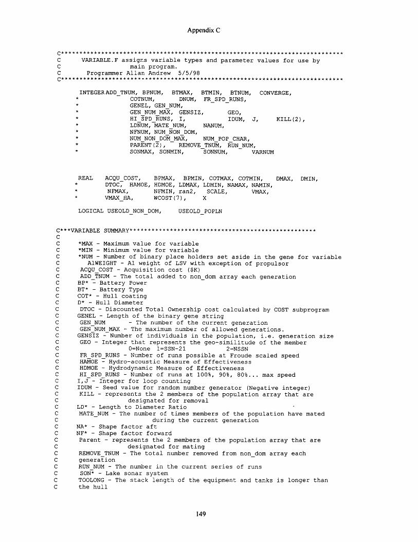
Appendix C
C VARIABLE.F assigns variable types and parameter values for use byC main program.C Programmer Allan Andrew 5/5/98
INTEGERADD TNUM, BPNUM, BTMAX, BTMIN, BTNUM, CONVERGE,* COTNUM, DNUM, FRSPDRUNS,* GENEL, GEN NUM,* GEN NUM MAX, GENSIZ, GEO,* HISPDRUNS, I, IDUM, J, KILL(2),* LDNUM, MATE NUM, NANUM,* NFNUM, NUM NON DOM,* NUM NON DOM_MAX, NUMPOPCHAR,* PARENT(2), REMOVETNUM, RUNNUM,* SONMAX, SONMIN, SONNUM, VARNUM
REAL ACQU_COST, BPMAX, BPMIN, COTMAX, COTMIN, DMAX, DMIN,* DTOC, HAMOE, HDMOE, LDMAX, LDMIN, NAMAX, NAMIN,* NFMAX, NFMIN, ran2, SCALE, VMAX,* VMAXHA, WCOST(7), X
LOGICAL USEOLDNONDOM, USEOLDPOPLN
C***VARIABLE SUMMARY***************************************************CC *MAX - Maximum value for variableC *MIN - Minimum value for variableC *NUM - Number of binary place holders set aside in the gene for variableC A1WEIGHT - Al weight of LSV with exception of propulsorC ACQU COST - Acquisition cost ($K)C ADD_TNUM - The total added to non dom array each generationC BP* - Battery PowerC BT* - Battery TypeC COT* - Hull coatingC D* - Hull DiameterC DTOC - Discounted Total Ownership cost calculated by COST subprogramC GENEL - Length of the binary gene stringC GEN NUM - The number of the current generationC GENNUM MAX - The maximum number of allowed generations.C GENSIZ - Number of individuals in the population, i.e. generation sizeC GEO - Integer that represents the geo-similitude of the memberC 0=None 1=SSN-21 2=NSSNC FRSPDRUNS - Number of runs possible at Froude scaled speedC HAMOE - Hydro-acoustic Measure of EffectivenessC HDMOE - Hydrodynamic Measure of EffectivenessC HI_SPD_RUNS - Number of runs at 100%, 90%, 80%... max speedC I,J - Integer for loop countingC IDUM - Seed value for random number generator (Negative integer)C KILL - represents the 2 members of the population array that areC designated for removalC LD* - Length to Diameter RatioC MATE_NUM - The number of times members of the population have matedC during the current generationC NA* - Shape factor aftC NF* - Shape factor forwardC Parent - represents the 2 members of the population array that areC designated for matingC REMOVE TNUM - The total number removed from non dom array eachC generationC RUN NUM - The number in the current series of runsC SON* - Lake sonar systemC TOOLONG - The stack length of the equipment and tanks is longer thanC the hull
149

Appendix C
C TOOHEAVY - The weight of the ship is greater than the displacementC USEOLD* - Logical variable to determine if old input data should beC used, or if new data should be generated to start the first generationC VARNUM - Number of variables in inputC VMAX - maximum LSV speedC VOLSUB - Total of hull volume and coating submerged to operating depthC WCOST - Seven weights to be used to calculate costC WPROP - Weight of the propulsorC X - Variable returned from random number generatorCC**************************************************************************w
C Seeds used for the random number generator:c DATA IDUM /-2589/
DATA IDUM /-4658/C DATA IDUM /-5346/C DATA IDUM /-9745/C DATA IDUM /-1896/
PARAMETER (DMIN=8.0, DMAX=15.0, LDMIN=6.0, LDMAX=13.0,NFMIN=1.75, NFMAX=4.00, NAMIN=1.75, NAMAX=4.00,BTMIN=1, BTMAX=4, BPMIN=3000.0, BPMAX=6500.0,COTMIN=0.0, COTMAX=3.5, SONMIN=l, SONMAX=2,DNUM=3, LDNUM=3, NFNUM=3, NANUM=3,BTNUM=2, BPNUM=4, COTNUM=3, SONNUM=1,VARNUM=8, GENEL=22, GENSIZ=200,NUMPOP CHAR=27, GEN NUM MAX = 160,NUM NON DOM MAX = 5000)
REAL BALANCE OUT(7), CHILD1(VARNUM), CHILD2(VARNUM),EXH SEARCH(3,184),NON DOM (NUM POP CHAR, NUM NON DOM MAX),MBR (VARNUM), MBR CHAR(NUM POP CHAR),CHILDI CHAR(NUM POPCHAR), CHILD2 CHAR(NUM POP CHAR),POPLN (NUM POP CHAR,GENSIZ),RANG (VARNUM, 3)
INTEGER BI_CHILD1(GENEL), BI CHILD2(GENEL),BIPOP (GENEL,GENSIZ), GENE (GENEL)
C BI_CHILD* - A child represented in binary form produced byC the mating of two parentsC BIPOP - An array of the binary code of each member of the populationC GENE is the binary string that represents a member of the populationC CHILD1(2) - Base 10 format of the binary string for child 1 or 2C MBR is the base 10 format of the binary stringC MBR_CHAR - The list of characteristics for each member randomlyC generatedC CHILD1(2)_CHAR - The list of characteristics for each member generatedC childC RANG is a 2-dimensional array that holds the min, max and length ofC the input variables
150
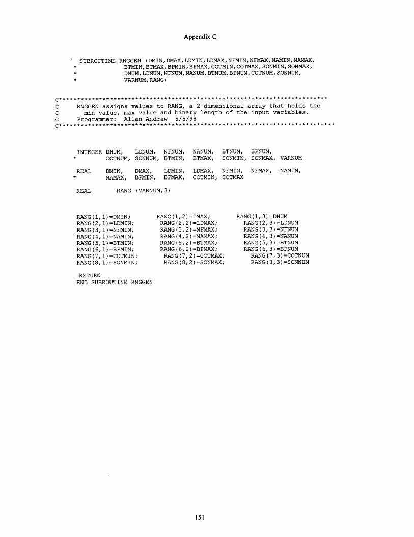
Appendix C
SUBROUTINE RNGGEN (DMIN,DMAX,LDMIN,LDMAX,NFMIN,NFMAX,NAMIN,NAMAX,* BTMIN,BTMAX,BPMIN,BPMAX,COTMIN,COTMAX,SONMIN,SONMAX,* DNUM,LDNUM,NFNUM,NANUM,BTNUM,BPNUM,COTNUM,SONNUM,* VARNUM,RANG)
C RNGGEN assigns values to RANG, a 2-dimensional array that holds theC min value, max value and binary length of the input variables.C Programmer: Allan Andrew 5/5/98C****************** ****************************************************
INTEGER DNUM, LDNUM, NFNUM,COTNUM, SONNUM, BTMIN,
NANUM, BTNUM, BPNUM,BTMAX, SONMIN, SONMAX, VARNUM
REAL DMIN, DMAX, LDMIN, LDMAX, NFMIN,* NAMAX, BPMIN, BPMAX, COTMIN, COTMAX
REAL
NFMAX, NAMIN,
RANG (VARNUM,3)
RANG (1, 1) =DMIN;RANG(2,1)=LDMIN;RANG (3,1)=NFMIN;RANG (4,1)=NAMIN;RANG(5, 1)=BTMIN;RANG (6, 1)=BPMIN;RANG(7,1)=COTMIN;RANG(8,1)=SONMIN;
RANG (1,2)=DMAX;RANG (2,2) =LDMAX;RANG (3,2)=NFMAX;RANG(4,2)=NAMAX;RANG (5,2)=BTMAX;RANG ( 6, 2) =BPMAX;
RANG (7,2)=COTMAX;RANG (8,2) =SONMAX;
RANG (1,3) =DNUMRANG (2,3) =LDNUMRANG (3,3)=NFNUMRANG (4, 3) =NANUMRANG (5,3)=BTNUMRANG (6,3)=BPNUM
RANG (7,3)=COTNUMRANG(8,3)=SONNUM
RETURNEND SUBROUTINE RNGGEN
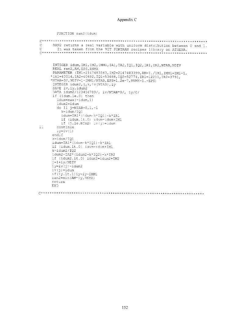
Appendix C
FUNCTION ran2(idum)
C RAN2 returns a real variable with uniform distribution between 0 and 1.C It was taken from the MIT FORTRAN recipes library on ATHENA.C*************************************
INTEGER idum,IM1,IM2,IMM1,IA1,IA2,IQ1,IQ2,IR1,IR2,NTAB,NDIVREAL ran2,AM,EPS,RNMXPARAMETER (IM1=2147483563,IM2=2147483399,AM=1./IM1,IMM1=IMl-1,
*IA1=40014,IA2=40692,IQl=53668,IQ2=52774,IRI=1221!,IR2=3791,*NTAB=32,NDIV=l-IMM/NTAB,EPS=1.2e-7,RNMX=I.-EPS)INTEGER idum2,j,k,iv(NTAB),iySAVE iv,iy,idum2DATA idum2/123456789/, iv/NTAB*0O/, iy/O/if (idum.le.0) then
idum=max(-idum,l)idum2=idumdo 11 j=NTAB+8,1,-1
k=idum/IQlidum=IAl*(idum-k*IQl)-k*IRlif (idum.lt.0) idum=idum+IM1if (j.le.NTAB) iv()=idum
11 continueiy=iv(l)
endifk=idum/IQ1idum=IAl*(idum-k*IQl)-k*IRlif (idum.lt.0) ioum=ldum+IM1k=idum2/IQ2idum2=IA2*(idum2-k*IQ2)-k*IR2if (idum2.1t.0) idum2=idum2+IM2j=!+iy/NDIViy=iv(j)-idum2iv(j)=idumIf(iy.It.1)iy=iy+IMM1ran2=min(AM*iy,RNMX)returnEND
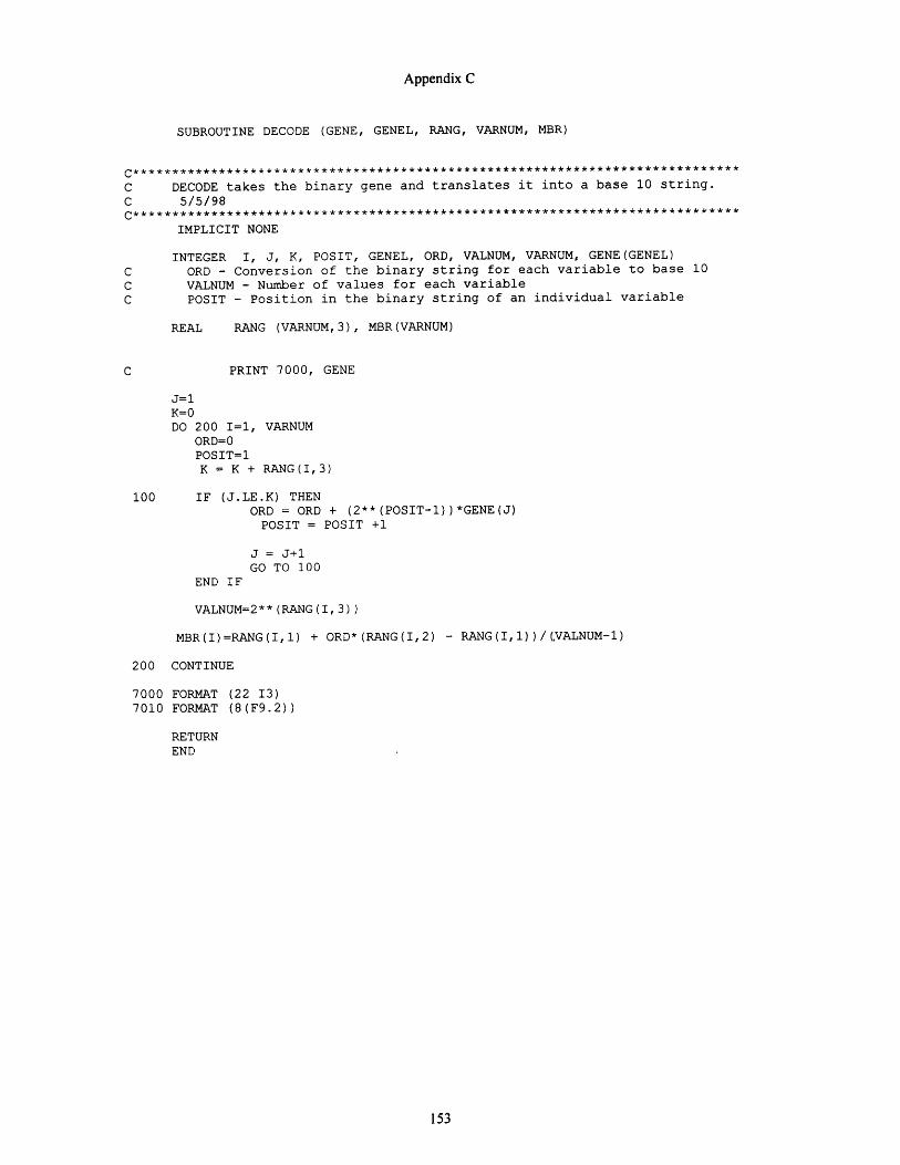
Appendix C
SUBROUTINE DECODE (GENE, GENEL, RANG, VARNUM, MBR)
C DECODE takes the binary gene and translates it into a base 10 string.
C 5/5/98**************************************************************************
IMPLICIT NONE
INTEGER I, J, K, POSIT, GENEL, ORD, VALNUM, VARNUM, GENE(GENEL)
C ORD - Conversion of the binary string for each variable to base 10
C VALNUM - Number of values for each variable
C POSIT - Position in the binary string of an individual variable
REAL RANG (VARNUM,3), MBR(VARNUM)
C PRINT 7000, GENE
J=1K=0DO 200 I=l, VARNUM
ORD=0POSIT=1K = K + RANG(I,3)
100 IF (J.LE.K) THENORD = ORD + (2**(POSIT-1))*GENE(J)POSIT = POSIT +1
J = J+1GO TO 100
END IF
VALNUM=2** (RANG (I, 3))
MBR(I)=RANG(I,l) + ORD*(RANG(I,2) - RANG(I,1))/(.VALNUM-1)
200 CONTINUE
7000 FORMAT (22 13)7010 FORMAT (8(F9.2))
RETURNEND
Appendix C
SUBROUTINE BALANCE (MBR, BALANCE OUT, WCOST)
C BALANCE takes a member of the population, determines if the member is aC feasible design, and returns member attributes.C Programmer: Allan Andrew 5/5/98C***************************
IMPLICIT NONE
REAL AlLCG, A1VCG, A1WEIGHT, BALANCE OUT(7), BP, COT, D, LBATT,LCB, LCGMBT, LD, LMBTA, LMBTF, LTRIM, NF, NA,VOLSUB, VOLTRIM, WSCOT, WCOST(7),WSHULL, WPROP
INTEGER BT
LOGICAL TOOLONG, TOOHEAVY
C AILCG - Longitudinal center of gravity in condition Al with propulsorC excludedC A1VCG - Vertical center of gravity with propulsor, hull coating andC lead excludedC A1WEIGHT - Al weight of LSV with exception of propulsorC LBATT - Length of the batteryC LCB - Longitudinal center of buoyancyC LCGMBT : Longitudinal Center of Gravity for filled MBT'SC LMBTA, LMBTF - Length of MBT aft and forwardC LTRIM : Length of the trim tankC TOOLONG - The stack length of the equipment and tanks is longer thanC the hullC TOOHEAVY - The weight of the ship is greater than the displacementC VOLSUB - Total of hull volume and coating submerged to operating depthC VOLMBTA, VOLMBTF - Volume of MBT's aft and forwardC VOLTRIM - Volume of the trim tankC WSHULL - Wetted surface areaC WPROP - Weight of the propulsor
REAL MBR(8)
C Assign input parameters from input arrays.D = MBR(1)LD = MBR(2)NF = MBR(3)NA = MBR(4)BT = NINT (MBR(S))BP = MBR(6)COT = MBR(7)
CALL CALC_GEOMETRY (D, LD, NA, NF, COT, VOLSUB, LCB,WSHULL, WSCOT, LMBTF, LMBTA, LTRIM, LCGMBT,VOLTRIM)
CALL CALC WEIGHT (D, LD, LMBTF, LMBTA, BT, BP, COT, WSHULL,A1WEIGHT, A1LCG, A1VCG, LBATT, WCOST)
CALL DET_FEAS (D, LD, LMBTF, LBATT, LTRIM, LMBTA, VOLSUB, LCB,A1WEIGHT, A1LCG, LCGMBT, TOOLONG, TOOHEAVY, WPROP)
C Assign output parameters to output array.BALANCE OUT(l) = VOLSUB/36.0BALANCE OUT(2) = AIWEIGHTBALANCE OUT(3) = WPROP
IF (TOOLONG) THENBALANCE OUT(4) = 1
ELSEBALANCE OUT(4) = 0
Appendix C
END IF
IF (TOOHEAVY) THENBALANCE OUT(5) = 1
ELSEBALANCE OUT(5) = 0
END IF
BALANCE OUT(6) = WSCOTBALANCEOUT(7) = VOLTRIM
RETURNEND SUBROUTINE BALANCE
C DET FEAS determines the feasibility of the design by ensuring theC length of all equipment fits in the hull and the weight is less
C than the displacement. It also determines the maximum propeller Cweight.
SUBROUTINE DETFEAS (D, LD, LMBTF, LBATT, LTRIM, LMBTA,VOLSUB,LCB,* A1WEIGHT, A1LCG, LCGMBT, TOOLONG, TOOHEAVY, WPROP)
IMPLICIT NONE
REAL A1LCG, A1WEIGHT, CONST, D, L, LCB, LD, LMBTF, LBATT,* LCGLEAD,LCGMBT, LCOMP, LTRIM, LMBTA, SUBDISP,* VOLSUB, WLEAD,WPROP
LOGICAL TOOLONG, TOOHEAVYC CONST - A place-holder representing constants in the propeller weightC calculationC LCGLEAD - Longitudinal center of gravity of the leadC LCOMP - Total component stack lengthC WLEAD - Weight of ballast and trim lead
C Calculate the total length of the MBT's, trim tank, battery, propulsionC motor and shafting (13ft), propulsion motor controller (12ft) andC electronic cabinets (12ft).
L = D*LD
LCOMP = LMBTF + LBATT + LTRIM + LMBTA + 37
IF (L .LT. LCOMP) THENTOOLONG = .TRUE.
ELSETOOLONG = .FALSE.
END IF
C Calculate the LSV displacement from submerged volume (freshwater 36C cubic ft / ton)and determine if the LSV weighs more than it C
displaces.
SUBDISP = VOLSUB / 36.0
C Calculate the maximum propulsor weight that can be carried. Assume all
C lead can be placed 5 feet aft of forward perpendicular.
LCGLEAD = 5.0CONST = SUBDISP*LCB - A1WEIGHT*A1LCG - 0.1*SUBDISP*LCGMBT
WPROP = (CONST - (SUBDISP-AlWEIGHT/0.9)*LCGLEAD)/(L-LCGLEAD)
IF (WPROP .LT. 0.0) THEN
155
Appendix C
TOOHEAVY = .TRUE.ELSE
TOOHEAVY = .FALSE.END IF
WLEAD = SUBDISP - AlWEIGHT/0.9 - WPROP
END SUBROUTINE DET FEAS
C*************************************************************************
C CALC_GEOMETRY calculates the volume, longitudinal center of buoyancy,C longitudinal center of gravity of main ballast tanks andC wetted surface area.C**********************************************************
SUBROUTINE CALC GEOMETRY (D, LD, NA, NF, COT, VOLSUB, LCB,WSHULL, WSCOT, LMBTF, LMBTA, LTRIM, LCGMBT,VOLTRIM)
IMPLICIT NONE
REAL COT, D, DCOT, DISPCHANGE, DISPSURF, DISPSUB, L,LA,LCB,LCGMBT,LCGMBTA, LCGMBTF, LF,LMBTA, LMBTF, LPMB, LD, LTRIM,MOMMBTA, MOMMBTF, NA, NF, PI, VMOMA, VMOMF, VMOMPMB, VOLA,VOLAI, VOLF, VOLFI, VOLPMB, VOLMBTA, VOLMBTF,VOLMOM,VOLHULL, VOLCOT, VOLSURF, VOLSUB, VOLTRIM, WSHULL, WSA,WSF, WSPMB, WSCOT, WSFCOT, WSPMBCOT, WSACOT
INTEGER DIVF, DIVA, I
C VARAIBLE DESCRIPTIONSC DCOT : Diameter with hull coatingC DISPSURF,DISPSUB,DISPCHANGE : Displacement on surface, submergedC and change betweenC surface and operating depthC L : Overall LengthC LA : Length aftC LCGMBTA, LCGMBTF : Longitudinal Center of Gravity for filled aftC and forward MBTC LF : Length forwardC LPMB : Length of parallel mid-bodyC MOMMBTA, MOMMBTF : Moment of aft and forward MBTC RA,RF : Radii of LSV at points of XA and XFC RACOT,RFCOT : Radii of LSV at points of XA and XF with coatingC VMOMA, VMOMF, VMOMPMB : Volume moment aft, forward, and PMBC VOLA, VOLF, VOLPMB : Volume of aft, forward, and parallelC mid-bodyC VOLAI, VOLFI : Volume of the ith portion of the aft,C forward, or PMBC VOLMOM : Total volume momentC VOLCOT : Volume of the hull coating on surfaceC VOLSUB : Volume of LSV with fully compressed hull coatingC VOLSURF : Volume of LSV on surface with uncompressed hull coatingC VOLHULL : Volume of hull without coatingC XA : Distance from stem for aft portion of LSVC XF : Distance from stem for forward portion of LSVc *COT : Variable with hull coating
PARAMETER (PI=3.1415926, DIVF=100, DIVA=100)
REAL XA(DIVA), XF(DIVF), RA(DIVA),RACOT(DIVA),RF(DIVF), RFCOT(DIVF)
Appendix C
L=LD*DLF=2.4*DLA=3.6*DLPMB=L-LF-LADCOT = D + 2.0*COT/12
C Determine longitudinal points to be evaluatedDO 100 I=1, DIVF
XF(I) = (I-1)*(LF/(DIVF-1))RF(I) = (D/2.0) * ((1.0 - ((LF-XF(I))/LF))**(1.0/NF))RFCOT(I) = (DCOT/2.0) * ((1.0 - ((LF-XF(I))/LF))**(1.0/NF))
100 CONTINUE
C PRINT *, 'RF = ',RF
DO 200 I=1, DIVAXA(I) = LF + LPMB + LA*(I-1)/(DIVA-1)
IF ( (XA(I)-LF-LPMB) .LT. 0.0) THENRA(I) = D/2.0RACOT(I) = DCOT/2.0
ELSERA(I) = (D/2.0) * ( 1- (((XA(I)-LF-LPMB) / LA)**NA))RACOT(I) = (DCOT/2.0)*( 1- (((XA(I)-LF-
LPMB)/LA) **NA))END IF
200 CONTINUEC PRINT *, 'RA = ',RA
C Calculate volumes, volume moments and wetted surface areasC forward, aft and parallel mid-body
VOLF = 0VMOMF = 0WSF = 0WSFCOT = 0DO 300 I=1, DIVF-1
VOLFI = (PI/4) * ((RF(I)+RF(I+1))**2) * (XF(I+1)-XF(I))VOLF = VOLF + VOLFIVMOMF = VMOMF + VOLFI * ( XF(I+1) + XF(I) ) / 2WSF = WSF + PI * (RF(I)+RF(I+1)) * (XF(I+1)-XF(I))WSFCOT = WSFCOT + PI * (RFCOT(I)+RFCOT(I+1)) * (XF(I+1)-XF(I))
300 CONTINUE
VOLA = 0VMOMA = 0WSA = 0WSACOT = 0DO 400 I=1, DIVA-1
VOLAI = (PI/4) * ((RA(I)+RA(i+1))**2) * (XA(I+1)-XA(I))VOLA = VOLA + VOLAIVMOMA = VMOMA + VOLAI * (LF + LPMB + (XF(I+1)+XF(I))/2)WSA = WSA + PI * (RA(I)+RA(i+1)) * (XA(I+1)-XA(I))WSACOT = WSACOT + PI * (RACOT(I)+RACOT(i+l)) * (XA(I+1)-XA(I))
400 CONTINUE
VOLPMB = (PI/4) * (D**2) * LPMBVMOMPMB = VOLPMB * (LF + LPMB/2)WSPMB = PI * D * LPMBWSPMBCOT = PI * DCOT * LPMB
C Calculate total volume, volume moment, LCB and wetted surface areaVOLHULL = VOLF + VOLA + VOLPMBVOLMOM = VMOMF + VMOMA + VMOMPMB
157
Appendix C
LCB = VOLMOM / VOLHULLWSHULL = WSF + WSPMB + WSAWSCOT = WSFCOT + WSPMBCOT + WSACOT
C Calculate the volume of the hull coating and the LSVC volume surfaced and submerged. Assume that theC hull coating compresses to 60% of its original volume.
VOLCOT = WSHULL*(COT/12)VOLSURF = VOLHULL + VOLCOTVOLSUB = VOLHULL + 0.6*VOLCOT
DISPSURF = VOLSURF/36.0DISPSUB = VOLSUB/36.0
DISPCHANGE = DISPSURF - DISPSUB
C Calculate the required trim tank size. Assume the trim tank isC 10% larger than the change in volume and uses 90% of the hullC volume. (36 cubic ft/ton fw)
VOLTRIM = 1.1 * DISPCHANGE * 36.0LTRIM = VOLTRIM / (0.9*(PI/4.0)*D**2)
C Calculate the lengths of the forward and aft main ballastC assuming the forward MBT is 7% and the aft MBT is 5% of theC total LSV volume of (1% in each for tank for equipment).
VOLMBTF = 0.0MOMMBTF = 0.0I=0
500 IF (VOLMBTF .LT. (0.07*VOLSUB)) THENI = I+1VOLMBTF = VOLMBTF+ (PI/4)*((RF(I)+RF(I+1))**2)*(XF(I+1)-XF(I))MOMMBTF = MOMMBTF+ (PI/4)*((RF(I)+RF(I+1))**2)*
(XF(I+1)-XF(I))* (XF(I+1)+XF(I))/2
GOTO 500END IF
LMBTF = LF * I / (DIVF-1)LCGMBTF = MOMMBTF/VOLMBTF
VOLMBTA = 0.0MOMMBTA = 0.0I= DIVA
600 IF (VOLMBTA .LT. (0.05VOLSUB)) THENI = I-1VOLMBTA = VOLMBTA+(PI/4)*((RA(I)+RA(I+1))**2)*(XA(I+1)-XA(I))MOMMBTA = MOMMBTA + (PI/4)*((RA(I)+BA(I+1))**2)*
(XA(I+1)-XA(I)) (XA(I+1)+XA(I))/2GOTO 600
END IFLMBTA = LA * (DIVA -I) / (DIVA-1)LCGMBTA = MOMMBTA/VOLMBTALCGMBT = 0.6*LCGMBTF + 0.4*LCGMBTA
RETURNEND SUBROUTINE CALC GEOMETRY
158
Appendix C
C***** ***************************************************************
C Subroutine CALC WEIGHT determines the weight, vertical center ofC gravity (VCG) and longitudinal center of LSV with the exception ofC propulsor, hull coating and lead
SUBROUTINE CALC WEIGHT (D,LD,LMBTF,LMBTA,BT,BP,COT,WSHULL,* A1WEIGHT, A1LCG, A1VCG, LBATT, WCOST)
IMPLICIT NONE
REAL D, LD, LMBTF, LMBTA, BP,COT, WSHULL, A1WEIGHT, A1LCG, A1VCG,* PI, L, Wl, LCG1, VCG1, W2, LCG2, VCG2,* W3, LCG3, VCG3,* BATT WT SP PWR(4), BATT VOL SP PWR(4),* WBATT, VBATT, LBATT, LCGBATT, VCGBATT,* WCABLE, LCGCABLE, VCGCABLE,* W3OTHER, LCG3OTHER, VCG3OTHER,* W4, LCG4, VCG4, W5, LCG5, VCG5, WCOOLING, W5OTHER,* W6, LCG6, VCG6, W7, LCG7, VCG7,* W6OTHER , WCOT, LCG6OTHER, LCGCOT, VCG6OTHER, VCGCOT,* WCOST(7)
INTEGER BT
C BATT VOL SP PWR - Battery specific power per unit volumeC BATT WT SP PWR - Battery specific power per unit weightC LCG* - Longitudinal center of gravity for group *C VCG* - Vertical center of gravity for group *C W* - Weight of group *
PARAMETER (PI=3.1415926)
L = D * LD
C Weight Group 1 (Structures)C Weight - ratio with LSV Al wetted surface areaC LSV Al W1 = 59.0 tonsC LSV Al WSHULL = 2920 sq ftC' LCG and LCV - use LSV Al ratio to L and DC
W1 = (59.0/2920.0)*WSHULLLCG1 = (0.489) * LVCG1 = (0.487) * D
C Weight Group 2 (Propulsion with exception of propulsor)C Weight - Same as LSV Al (16.2 tons)C LCG - 9 ft. forward of aft pressure hullC (Same location as LSV Al)C VCG - LSV Al VCG/D ratio
W2 = 16.2LCG2 = L - LMBTA - 9VCG2 = 0.5 * D
C Weight Group 3 (Electric Plant)C Weight- Battery: Power divided by specific power per weightC Cable: Distance from battery center to motor controllerC multiplied by cable density from LSV Al.C Other: Same as LSV Al (2.3 tons)C LCG- Battery: Assume battery uses 40% of available space and
C starts 2 ft. aft of forward MBT.C Cable: Half-way between battery center and motor C
controller.C Other: LSV Al LCG/L ratio (0.45)
159
Appendix C
C VCG - LSV Al VCG/D ratio: Battery (0.43)C Cable (0.55)C Other (0.45)C Battery volume- Power divided by specific power per volume.C Battery Length (LBATT)- Assume 20% of the hull can be used forC battery. (65% for structures and spacing from LSV AlC drawing 15% for cooling from GNB paper)
BATT WT SP PWR (1) = 45.2BATT WT SP PWR (2) = 62.2BATT WT SP PWR (3) = 106.6BATT WT SP PWR (4) = 181.6
BATT VOL SP PWR (1) = 4.87BATT VOL SP PWR (2) = 5.70BATT VOL SP PWR (3) = 5.0BATT VOL SP PWR (4) = 13.8
WBATT = BP / BATT WT SP PWR (BT)VBATT = BP / BATT VOL SP PWR (BT)LBATT = ((VBATT)/0.2) / ((PI/4.0)*(D**2))LCGBATT = LMBTF t 2.0 + LBATT/2.0VCGBATT= (0.43)* D
WCABLE = (5.0/(70.0-33.0)) *(L-LMBTA-22.0-LCGBATT)
LCGCABLE = (L-LMBTA-2+LCGBATT) / 2.0VCGCABLE = (0.55) * D
W30THER = 2.3LCG3OTHER = 0.45 * DVCG3OTHER = 0.5 * D
W3 = WBATT + WCABLE + W30THERLCG3 = (WBATT*LCGBATT + WCABLE*LCGCABLE + W30THER*LCG30THER)/W3VCG3 = (WBATT*VCGBATT + WCABLE*VCGCABLE + W30THER*VCG30THER)/W3
C Weight Group 4 (Command and Control)C Weight - Same as LSV Al (6.5 tons)C LCG - 26 ft forward of aft MBTC VCG - LSV Al VCG/D ratio (0.5)
W4 = 6.5LCG4 = L- LMBTA - 26.0VCG4 = 0.5 * D
C Weight Group 5 (Auxiliaries)C Weight- Cooling: LSV Al Weight/Battery Power ratio
(2.5 tons, 2673 kw)C Other: LSV Al Weight/Length ratioC (6.1 tons, 110 feet)C LCG- 26 feet forward of aft MBTC VCG- LSV Al VCG/D ratio (0.5)
WCOOLING = (2.5 / 2673.0) * BPW5OTHER = (6.1 / 110.0) * LW5 = WCOOLING + WSOTHER
LCG5 = L - LMBTA - 26.0VCG5 = 0.5 * D
C Weight Group 6 (Outfit and Furnishings)C Weight- Other: LSV Al Weight/Length ratioC (2 tons, 110 feet)C Hull Coating: 60 cubic feet / tonC with uncompressed volume equal toC wetted surface area multiplied by
Appendix C
C coating thickness.
C LCG- Other: LSV Al LCG/L ratio (0.62)
C Hull Coating: Same as LCG for W1
C VCG- Other: LSV Al VCG/D ratio (0.45)
C Hull Coating: Center line
W6OTHER = (2.0 / 110.0) * LWCOT = WSHULL * (COT/12.0) / 60.0
LCG6OTHER = 0.62 * LLCGCOT = 0.489 * L
VCG6OTHER = 0.45 *DVCGCOT = 0.5 * D
W6 = W6OTHER + WCOT
LCG6 = (W6OTHER*LCG6OTHER + WCOT*LCGCOT) / W6
VCG6 = (W6OTHER*VCG6OTHER + WCOT*VCGCOT) / W6
C Weight Group 7 (Instrumentation)C Weight - LSV Al Weight/Length ratio (2.23 tons, ll0ft)
C LCG - LSV Al LCG/L ratio (0.53)C VCG - LSV Al VCG/D ratio (0.5)
W7 = (2.23/110.0) * LLCG7 = 0.53 * LVCG7 = 0.5 * D
C Calculate total weight, LCG and VCG
A1WEIGHT = W1 + W2 + W3 + W4 + W5 + W6 + W7
A1LCG = (Wl*LCG1 + W2*LCG2 + W3*LCG3 t W4*LCG4 + W5*LCG5 +
W6*LCG6 + W7*LCG7) / A1WEIGHTA1VCG = (Wl*VCG1 + W2*VCG2 + W3*VCG3 + W4*VCG4 + W5*VCG5 +
W6*VCG6 + W7*VCG7) / A1WEIGHT
C Assign weights to the array used in cost calculation
WCOST(1) = W1WCOST(2) = WBATTWCOST(3) = W30THERWCOST(4) = WCOOLINGWCOST(5) = W5OTHERWCOST(6) = WCOTWCOST(7) = W6OTHER
END SUBROUTINE CALC WEIGHT

Appendix C
SUBROUTINE COST (MBR, WCOST, BALANCE OUT, DTOC, ACQU COST)
C Subroutine COST calculates total ownership cost from batterytype, battery power and various weight groups.Note: All costs are in thousands of FY97 dollars
C Programmer: Allan AndrewC 5/5/98
IMPLICIT NONE
REAL ACQU COST,BP, BPCER,COTCOST,DF20, DF1 20,DTOC, MBR(8),VOLCOT,W30THER,W50THER,W6OTHER,WCOOLING,WCOST(7),WSCOT, WSCOTCEYEARLY COST
INTEGER BT, I,
BALANCE OUT (7),BPCOST, CONSTANT COST,DF3 20, DF5, DF10, DFl5,
DR, DISPOSAL COST,SONARCOST, UPGRD COST,
VOLCOTCER, W1, W1CER, W1COST,W30THERCER, W30THERCOST,W5OTHERCER, WSOTHERCOST,W60THERCER, W60THERCOST,WCOOLINGCER, WCOOLINGCOST,
ER,
SONAR
*CER - Cost estimating relationship for *W*CER - $K/TONBPCER - $K/kWVOLCOTCER - $K/ft^3WSCOTCER - $K/ft^2
CONSTANT_COST - Portion of acquisition cost that is the same for allvariants of LSV
DISPOSAL COST - Cost of disposal of LSV at end of lifeDR - Discount rate used to calculate discounted total ownership costDF* - Discount factor for * years
3 20 is DF for battery replacement every 3 yearsUPGRD COST - Discounted cost of upgrades for GNC and new batteries.YEARLY COST - Total discounted yearly costs of operating the LSV
PARAMETER (BPCER=0.746, W1CER-W50THERCER=763.0,WCOOLINGCER=763.0,WSCOTCER=0.234,
76.0, W30THERCER=171.0,W60THERCER=683.0,VOLCOTCER=0.897,DR = 0.C6)
BT = INT (MBR(5))
BP = MBR(6)SONAR = INT (MBR(8))
Wl = WCOST(1)
W30THER = WCOST(3)WCOOLING = WCOST(4)
W5OTHER = WCOST(5)W6OTHER = WCOST(7)
WSCOT = BALANCE OUT(6)COT = MBR(7)VOLCOT = WSCOT * COT / 12.0
C Calculate discount factors for 5,C a 20 year annuity
10, 15, 20 years and
DF3 20 = 1/((1+DR)**3) + i/((1+DR)**6) + l/((1+DR)**9) +1/((1+DR)**12) + 1/((1+DR)**15) + /((l1+DR)**18)
162
COT,
Appendix C
DF5 = 1/((l+DR)**5)DF10 = 1/((1+DR)**10)DF15 = 1/((l+DR)**15)DF20 = 1/((1+DR)**20)DF1 20 = 0I = 0
100 IF (I.LT.20) THENI = I+1DF1 20 = DF1 20 + 1/((l+DR)**I)GOTO 100
END IF
C Determine cost of each portion of LSV by multiplying the SWBS weightC with the cost estimating relationship (CER)
CONSTANT COST = 28230.0W1COST = W1CER * W1W30THERCOST = W30THERCER * W30THERWCOOLINGCOST = WCOOLINGCER * WCOOLINGW5OTHERCOST = W5OTHERCER * W5OTHERCOTCOST = WSCOTCER * WSCOT + VOLCOTCER * VOLCOT
C PRINT *, 'COTCOST = ', COTCOSTW6OTHERCOST = W6OTHERCER * W6OTHER
IF (BT.EQ.1)THENBPCOST = BPCER * BP * 1.0UPGRD COST = (1100.0 ) * (DF5 + DF10 + DF15)
+ BPCOST * DF3 20ELSE IF (BT.EQ.2) THEN
BPCOST = BPCER * BP * 1.0UPGRD COST = 1100.0*(DF5 + DF10 + DF15) + BPCOST*DF1 20
ELSE IF (BT.EQ.3) THENBPCOST = BPCER * BP * 1.5UPGRD COST = (1100.0 ) * (DF5 + DF10 + DF15)
* + BPCOST * DF3 20
ELSE IF (BT.EQ.4) THENBPCOST = BPCER * BP * 2UPGRD COST = (1100.0 ) * (DF5 + DF10 + DF15)
+ BPCOST * DF3 20END IF
C Calculate acquisition cost with 10% profit margin
ACQU COST = (CONSTANT COST + W1COST + W30THERCOST +* WCOOLINGCOST + W5OTHERCOST + COTCOST + W6OTHERCOST +* BPCOST)*1.1
C Assume no additional cost if current sonar system is used.C Assume $3M dollar investment if sonar system is upgraded.
IF (SONAR.EQ.1) THENSONARCOST = 0
ELSE IF (SONAR.EQ.2) THENSONARCOST = 3000.0
END IF
C Assume yearly operating expenses of $7.17M.YEARLY COST = DF1 20 * 7170.0
C Assume disposal cost of $1M.DISPOSAL COST = DF20 * 1000.0
DTOC = ACQU COST + SONARCOST + YEARLY COST+ DISPOSAL COST + UPGRD COST
END SUBROUTINE COST
163
Appendix C
SUBROUTINE CALC HA MOE (VMAX, HISPD RUNS, MBR, HAMOE)
C****************** ******f**
C Subroutine CALC HA MOE calculates the hydro-acoustic measures ofC effectiveness for each member of the LSV populationC Programmer: Allan AndrewC 5/5/98C********************************************************************
IMPLICIT NONE
REAL COT, ERROR, HAMOE, MBR(8), V2, V3, VMAX
INTEGER HI SPD RUNS, SON
C ERROR - A measure of the expected maximum error in measurement ofC the LSV acoustic signatureC V2 - The speed of the final high speed runC V3 - The speed to which it is desired to extrapolate theC acoustic data
PARAMETER (V3 = 15.0)
COT = MBR(7)SON = MBR(8)
C Calculate the error band.
ERROR i1.0 / (SON * (COT+1.0))
C PRINT *, 'ERROR = ', ERROR
IF (HI SPD RUNS .LE. 1) THENHAMOE = 10
ELSEV2 = 18.5
HAMOE = 2 ' ERROR * (LOG10(SQRT(VMAX*V2)/V3)) /(LOG10(SQRT(VMAX/V2)))
END IF
END SUBROUTINE CALC HA MOE
164
Appendix C
SUBROUTINE CALC HD MOE (MBR, BALANCEOUT, FRSPDRUNS, HDMOE, GEO)
C Subroutine CALC HD MOE calculates the hydrodynamic measures ofC effectiveness for each member of the LSV populationC Programmer: Allan AndrewC 5/5/98C** ********************** **********
IMPLICIT NONE
REAL BALANCE OUT(7), HDMOE, DMOE1,* DMOE2, LD, MARGIN, MBR(8), MARGIN HD,* MARG1(7,4), MARG2(6,3), MARTH, MARGOAL, NA, NF
INTEGER FRSPD RUNS, FSRHD, FSRTH, FSRGOAL,* GEO, I, J, K, L
C*****Variables***************************************************************Cc HDMOE - Total Hydrodynamic MOEC DMOE1 - Hydrodynamic MOE for FR SPD RUNSC DMOE2 - Hydrodynamic MOE for Geo-simmilitudeC FR SPD RUNS - Number of times the member can complete the sonar courseC at Froude scaled speedC FSRHD - Number of Froude speed runs used to calculate HD MOEC FSRTH - The threshold for minimum FR SPD RUNSC GEO - Integer that represents the geo-similitude of the memberC 0=None 1=SSN-21 2=NSSNC I - Counter in MARG1 that represents Iso-Value lineC J - Counter in MARG1 that represents FR SPEED RUNSC K - Counter in MARG2 that represents Iso-Value lineC L - Counter in MARG1 that represents Geo-SimilitudeC MARGIN HD - Margin used to calculate HD MOEC MARG1 - Array that contains the equivalent values of margin for changesC in number of Froude speed runsC MARG2 - Array that contains the equivalent values of margin for changesC in geo-similitudeC MARGIN - Maximum weight that can be added at stern of member includingC propulsor
C Assign the values to MARG1 and MARG2 determined from MAIE survey.
MARG1(1,1)=.03; MARG1(1,2)=0.0; MARG1(1,3)=0.0; MARGl(1,4)=O.O;MARG1(2,1)=.035; MARG1(2,2)=.03; MARGl(2,3)=0.0; MARGl(2,4)=0.0;MARG1(3,1)=.05; MARGl(3,2)=.04; MARG1(3,3)=.03; MARG1(3,4)=0.0;MARG1(4,1)=.06; MARG1(4,2)=.05; MARG1(4,3)=.04; MARGl(4,4)=.03;MARG1(5,1)=.09; MARG1(5,2)=.08; MARG1(5,3)=.07; MARG1(5,4)=.06;MARGl(6,1)=.12;MARGl(6,2)=.11;MARG1(6,3)=.10;MARGl(6,4)=.09;MARG1(7,4)=.12
MARGl(7,3)=MARG1(7,4) + MARG1(6,3) - MARG1(6,4)MARG1(7,2)=MARG1(7,4) + MARG1(6,2) - MARGl(6,4)MARGl(7,1)=MARG1(7,4) + MARGl(6,1) - MARG1(6,4)
MARG2(1,1)=.03; MARG2(1,2)=0.0; MARG2(1,3)=0.0MARG2(2,1)=.04; MARG2(2,2)=.03; MARG2(2, 3)=0.0MARG2(3,1)=.05; MARG2(3,2)=.04; MARG2(3,3)=.03MARG2(4,1)=.08; MARG2(4,2)=.07; MARG2(4,3)=.06MARG2(5,1)=.11; MARG2(5,2)=.10; MARG2(5,3)=.09MARG2 (6, 3)=.12MARG2(6,2)=MARG2(6,3) + MARG2(5,2) - MARG2(5,3)MARG2(6,1)=MARG2(6,3) + MARG2(5,1) - MARG2(5,3)
C Assign the values for the MOPSMARGIN = BALANCE OUT(3) / BALANCE OUT(1)
165
Appendix C
C Determine the GEOSIM hull formLD = MBR(2)NF = MBR(3)NA = MBR(4)
C NSSN IF:IF ((LD .GE. 10.0) .AND. (LD .LE. 12.0) .AND.
* (NF .GE. 2.25) .AND. (NF .LE. 2.75) .AND.* (NA .GE. 2.5) .AND. (NA .LE. 3.0)) THEN
GEO = 2
C SSN-21 IF:ELSE IF ((LD .GE. 7.0) .AND. (LD .LE. 9.0) .AND.
* (NF .GE. 2.5) .AND. (NF .LE. 3.0) .AND.* (NA .GE. 2.75) .AND. (NA .LE. 3.25)) THEN
GEO = 1
C Otherwise no Geo-simnELSE
GEO = 0END IF
C Calculate Hydrodynamic MOE for Froude Speed Runs
C Enter the goals and thresholdsFSRTH = 7; FSRGOAL = 10
MARTH = .03; MARGOAL = .12
C If number of Froude speed runs or margin less than the threshold,C set the MOE for Froude speed runs to zero.
IF ( (FR SPD RUNS .LT. FSRTH) .OR. (MARGIN .LT. MARTH) ) THENHDMOE = 0.0GOTO 1000
END IF
C If number of Froude speed runs or margin greater than goal, reduceC its value to the goal.
IF (FR SPD RUNS .GT. FSRGOAL) THENFSRHD = FSRGOAL
ELSEFSRHD = FR SPD RUNS
END IF
C WRITE (99,*) 'FSRHD = ', FSRHD
IF (MARGIN .GT. MARGOAL) THENMARGIN HD = MARGOAL
ELSEMAPGIN HD = MARGIN
END IF
C WRITE (99,*) 'MARSIN HD = ', MARGIN HD
C Set the value of J to enter MARG1 matrix.J = FSRHD - FSRTH + 1
C Search the MARG1 matrix for the value of Froude speed runs and margin.C Interpolate and return the equivalent margin for threshold ofC Froude speed runs.
I = 1
100 IF ( MARGIN HD .LE. MARG1(I+1,J) ) THEN
Appendix C
DMOE1 = (MARGIN HD - MARG1(I,J))*(MARGl(I+l,1) - MARGl(I,1))/(MARGl(I+1,J) - MARGl(I,J)) + MARGl(I,1)
ELSEI = I+1GOTO 100
END IF
C WRITE (99,*) 'DMOE1 = ',DMOE1
C Set the value of L to enter MARG2 matrixL = GEO + 1
C Search the MARG2 matrix for the value of Froude speed runs andC Geo-similitude. Interpolate and return the CHANGE in equivalentC margin from threshold Geo-sim.
K = 1
200 IF ( MARGIN HD .LE. MARG1(K+1,L) ) THEN
DMOE2=((MARGIN HD - MARG2(K,L))*(MARG2(K+1,1) - MARG2(K,1))/* (MARG2(K+1,L) - MARG2(K,L)) + MARG2(K,1)) -* MARGIN HD
ELSEK = K+lGOTO 200
END IF
HDMOE = DMOE1 + DMOE2
1000 CONTINUE
7010 FORMAT (7(F9.2))7020 FORMAT (6(F9.2))
END SUBROUTINE CALC HD MOE
167
Appendix C
SUBROUTINE REPLACE (BIPOP, GENE, GENEL, POPLN, NUM POP CHAR,GENSIZ, REPLACE NUM, DTOC, HAMOE, HDMOE,MBR, VARNUM, BALANCE OUT, FR SPD RUNS,HI SPD RUNS, VMAX,GEO, ACQU COST, GEN NUM, GEN NUM MAX,RUN NUM, MBR CHAR, VMAX HA, SCALE)
C Replace takes member or child and inserts it into the populationC and binary population arrays.CC Programmer: Allan Andrew 5/5/98
IMPLICIT NONE
INTEGER FR SPD RUNS, GENEL, GEN NUM,GEN NUM HI, GEN NUM LO, GEN NUM MAX,GENSIZ, BIPOP(GENEL,GENSIZ),GENE(GENEL), HI SPD RUNS,I, J, GEO, NUM POP CHAR,REPLACE NUM, RUN NUM, VARNUM
REAL ACQU COST, BALANCE OUT(7), DTOC,HAMOE, HDMOE, MBR(VARNUM), MBR CHAR(NUM POP CHAR),PENALTY, PENALTY MAX,POPLN(NUM POP CHAR, GENSIZ), SCALE,VMAX, VMAX HA
DO 200 I=1, GENELBIPOP(I, REPLACE NUM) = GENE(I)
200 CONTINUE
DO 210 J=4, VARNUM+3POPLN(J,REPLACE NUM)
CONTINUE
POPLN(12,REPLACE NUM)POPLN(13,REPLACE NUM)POPLN(14,REPLACE NUM)POPLN(15,REPLACE NUM)POPLN(16,REPLACE NUM)POPLN(17,REPLACE NUM)POPLN(18,REPLACE NUM)POPLN(19,REPLACE NUM)POPLN(20,REPLACE NUM)POPLN(21,REPLACE NUM)
POPLN(22,REPLACE NUM)POPLN(23,REPLACE NUM)POPLN(24,REPLACE NUM)POPLN(25,REPLACE NUM)POPLN(26,REPLACE NUM)POPLN(27,REPLACE NUM)
= MBR(J-3)
= BALANCE OUT(1)= BALANCE OUT(3)= BALANCE OUT(4)= BALANCE OUT(5)
FR SPD RUNSHI SPD RUNS
= VMAX= GEO= ACQU COST/1000= GEN NUM
= DTOC/1000= HAMOE= -HDMOE= RUN NUM= VMAX HA= SCALE
GEN NUM LO = NINT(0.2*GEN NUM MAX)GEN NUM HI = NINT(0.8*GEN-NUM MAX)
PENALTY MAX = 10
IF (GEN NUM .LT. GEN NUM LO) THENPENALTY = 1.0
ELSE IF ((GEN NUM .GE. GEN NUM LO)
210
.AND.
Appendix C
(GEN NUM .LE. GEN NUM HI)) THENPENALTY = 10 ** ((LOG1O(PENALTY MAX)) * (GEN NUM - GEN NUM LO)/
(GEN NUM HI - GEN NUM LO))
ELSEPENALTY = 10**6
END IF
IF ( (POPLN(14,REPLACE NUM) .EQ. 1.0) .OR.
(POPLN(15,REPLACE NUM) .EQ. 1.0) ) THEN
POPLN(1,REPLACE NUM) = NINT ((DTOC/1000) * PENALTY)POPLN(2,REPLACE NUM) = (FLOAT(NINT(1000*HAMOE * PENALTY)))/1000POPLN(3,REPLACE-NUM)=-(FLOAT(NINT(1000*HDMOE / PENALTY)))/1000
POPLN(1,REPLACE NUM)POPLN(2,REPLACE NUM)POPLN(3,REPLACE-NUM)
= NINT(DTOC/1000)= (FLOAT(NINT(1000*HAMOE)) )/1000= -(FLOAT(NINT(1000*HDMOE)) )/1000
DO I=l, NUM POP CHARMBR CHAR(I) = POPLN(I,REPLACENUM)
END DO
END SUBROUTINE REPLACE
ELSE
END IF
Appendix C
SUBROUTINE NONDOMINATED (MBRCHAR, NUM POP CHAR,NON_DOM, NUM NON DOM MAX, NUM NON DOM,ADDTNUM, REMOVE TNUM, EXH SEARCH)
C* * ************************************* *****************
C Subroutine NON DOMINATED stores all members that are on the non-C dominated frontier.C Programmer: Allan Andrew 5/5/98
IMPLICIT NONE
INTEGER ADD_TNUM, COUNTER, I, J,NUMBERFOUND, NUM NON DOM, NUM NON DOM MAX,NUM POP CHAR, NUM REMOVE, REMOVE TNUM
REAL NON DOM (NUM POP CHAR, NUM NON DOM MAX),EXH SEARCH(3, 184), PENALTY,MBR CHAR (NUM POP CHAR)
INTEGER REMOVE(NUM NON DOM MAX)
LOGICAL CLONE, NEW_MBR, NON DO MMBR, ND MBR ADDED,ND MBR FOUND
C ADD - An array that stores the location of the members of the POPLNC array that are to be added to the Non-Dom arrayC CLONE - Logical variable to determine if member is clone of non-domC COUNTER - Counts the number of times the subroutine has been calledC NEW MBR - Logical variable to determine if a member with the sameC MOE's and cost is different typeC NUMADD - The number of members from the population array that are toC be added to the Non-Dom array.C NON DOM - The array that holds the characteristics of the don-dominatedC inaividualsC NON DOM MBR - A logical variable that is true if the member of theC population is non-dominated and false if dominated.C NUM NON DOM - The number of non-dominated IndividualsC NUM REMOVE - The number of individuals to be removed from the Non-DomC arrayC PENALTY - The max penalty applied if the variant is too long or tooC heavyC PREVIOUSLY REMOVED - Logical variable that determines if a member hasC been already been marked for removal from the populationC REMOVE - An array that stores the location of the members of the Non-C Dom array that are to be removed because they areC dominated by new individuals
ND MBR ADDED = .FALSE.
COUNTER = COUNTER + 1
C Apply the maximum penalty to the MOE's and cost if the variant isC infeasible.
IF ( (MBRCHAR(14) .EQ. 1.0).OR.(MBR CHAR(15) .EQ. 1.0).OR. (MBR CHAR(17) .LE. 1)) THENMBR CHAR(1) = 100000000MBR CHAR(2) = 100000000MBR-CHAR(3) = 100000000
END IF
C If there are no members in the non-dominated array, place the
170

Appendix C
C the member in the non-dom array.
IF (NUM NONDOM .EQ. 0) THEN
NUM NON DOM = NUM NON DOM + 1ADD TNUM = ADD TNUM + 1ND MBR ADDED = .TRUE.
DO J=l, NUM POP CHARNON DOM(J,NUM NON DOM) = MBR CHAR(J)
END DO
C If there are already members in the non-dominated array, compareC the member to determine if it should be inserted and which
C members should be removed from the non-dominated array.
ELSE
NUM REMOVE = 0
IF ( (MBR CHAR(1) .GE. NON DOM(1,J)).AND. (MBR CHAR(2) .GE. NON DOM(2,J))
* .AND. (MBR CHAR(3) .GE. NON DOM(3,J)) ) THENNON DOM MBR = .FALSE.
END IF200 CONTINUE
IF (NON DOM MBR) THENDO 300 J=l, NUM NON DOM
IF ( (MBR CHAR(l) .LE. NON DOM(1,J))* .AND. (MBR CHAR(2) .LE. NON DOM(2,J))* .AND. (MBR CHAR(3) .LE. NON DOM(3,J)) ) THE
NUM REMOVE = NUM REMOVE + 1REMOVE (NUM REMOVE) = J
END IF300 CONTINUE
IF (NUM REMOVE .EQ. 1) THENDO J=l, NUM POP CHAR
NON DOM(J, REMOVE(1)) = MBR CHAR(J)END DO
ELSE IF (NUM REMOVE .GT. 1) THENDO J=l, NUM POP CHAR
NON DOM(J, REMOVE(1)) = MBR CHAR(J)END DODO I = 2, NUM REMOVE
DO J=l, NUM POP CHARNON DOM(J, REMOVE(I)) =NON DOM(J, NUM NON DOM - I + 2)
END DOEND DO
ELSE IF (NUM REMOVE .EQ. 0) THENDO J=l, NUM POP CHAR
NON DOM(J, NUM NON DOM + 1) = MBR CHAR (J)END DO
END IF
NUM NON DOM = NUM NON DOM + 1 - NUM REMOVEADD TNUM = ADD TNUM + 1ND MBR ADDED = .TRUE.REMOVE-TNUM = REMOVE TNUM + NUM REMOVE
ELSECLONE = .FALSE.NEW MBR = .FALSE.DO 1000 J=l, NUM NON DOM
IF ( (MBR CHAR(l) .EQ. NON DOM(1,J))
Appendix C
(MBR CHAR(2)(MBR CHAR(3)
IF.AND. (MBR CHAR(5).AND. (MBR CHAR(6).AND. (MBR CHAR(7).AND. (MBR CHAR(8).AND. (MBR CHAR(9).AND. (MBR CHAR(10).AND. (MBR CHAR(11)
.EQ. NON DOM(2,J))
.EQ. NON DOM(3,J)) ) THEN
(MBR CHAR(4) .EQ. NON DOM(4,J)).EQ. NON DOM(5,J)).EQ. NON DOM(6,J)).EQ. NON DOM(7,J)).EQ. NON DOM(8,J)).EQ. NON DOM(9,J)).EQ. NON DOM(10,J)).EQ. NON DOM(11,J)) ) THEN
CLONE = .TRUE.
NEW MBR = .TRUE.
END IFEND IF
CONTINUE
IF ((NEW MBR) .AND. (.NOT. CLONE)) THEN
DO J=1, NUM POP CHARNON DOM(J, NUM NON DOM + 1) =
END DOMBR CHAR (J)
NUM NON DOM = NUM NON DOM + 1ADD TNUM = ADD TNUM + 1ND MBR ADDED = .TRUE.
END IF
END IF
END IF
ND MBR FOUND = .FALSE.
IF (ND MBR ADDED) THENDO I=l, 326
END DO
IF (.AND..AND.
END IF
(MBR CHAR(1) .EQ. EXH SEARCH(1,I))(MBR CHAR(2) .EQ. EXH SEARCH(2,I))(MBR CHAP(3) .EQ. EXH SEARCH(3,I)) ) THENND MBR FOUND = .TRUE.
IF (ND MBR FOUND) THENNUMBER FOUND = NUMBER FOUND + 1WRITE (72,*) NUMBER FOUND, COUNTERprint *, 'NBR FOUND/COUNTER',NUMBER FOUND, COUNTER
END IF
END IF
C WRITE (32, *) NUM ADD, NUM REMOVE, NUM NON DOM
7020 FORMAT (25(F10.3))
RETURNEND SUBROUTINE NON DOMINATED
172
.AND.
.AND.
ELSE
1000
Appendix C
SUBROUTINE TOURNAMENT (POPLN, NUMPOP CHAR, GENSIZ,* IDUM, PARENT, KILL)
C*** ********** ******* ***************************************************
C Subroutine TOURNAMENT takes the population array and selectsC 2 members for parents and 2 members for removal.CC Programmer: Allan Andrew 5/5/98
*****************************************************************************
IMPLICIT NONE
INTEGER GENSIZ, COUNT, DOMARR(GENSIZ,GENSIZ), HI NICHE,* I, IDUM, J, KILL(2), LEAST, LOC HI NICHE(GENSIZ),* LOC LOW NICHE(GENSIZ), LOSER(GENSIZ),* LOSSES, LOW NICHE, MOST, NICHE COUNT(GENSIZ),* NUM HI NICHE, NUM LOW NICHE, NUMPOPCHAR,* PARENT(2), TNUM,* TSIZE, TVEC(GENSIZ), WINNER(GENSIZ), WINS
REAL POPLN(NUM_POPCHAR,GENSIZ), RAN2
C COUNT - A count of the number of other members that dominate anC individualC DOMARR - Represents the dominance of members of the population arrayC with respect to other members.C If "I" dominates "J", thenC DOMARR(I,J) = +1C DOMARR(J,I) = -1C If neither member dominates, thenC DOMARR(I,J) = 0C LOSER - The numbers of the members that loose the tournamentC LOSSES - The number of members that loose the tournamentC TNUM - The number of the tournament (1 or 2)C TSIZE - Tournament sizeC WINNER - The numbers of the members that win the tournamentC WINS - The number of members that win the tournament
C Calculate how many individuals are "close" to each individual inC effectiveness/cost space.
CALL NICHE (POPLN, NUM POPCHAR, GENSIZ, NICHECOUNT)
C Choose the tournament size to be a fraction of the generation size
TSIZE = NINT (0.1*GENSIZ)
C Randomly select tournament contestants.
TNUM=l
50 DO I=l, TSIZE100 TVEC(I) = INT(ran2(IDUM) * FLOAT(GENSIZ-1)) + 1
C Prevent duplicate selectionsDO J=l, I-1
IF (TVEC(J) .EQ. TVEC(I)) GOTO 100END DO
END DO
C Zero the dominance array and winner/loser vectorsDO I = 1,GENSIZ
WINNER(I) = 0LOSER(I) = 0DO J = 1,GENSIZ
DOMARR(I,J) = 0END DO
Appendix C
END DO
Construct the dominance array using only the tournamentcontestants.
DO I = 1,TSIZE-1DO J = I+1,TSIZE
IF((POPLN(1, TVEC(I))POPLN(2, TVEC(I))POPLN(3, TVEC(I))
.OR.(POPLN(1, TVEC(I))POPLN(2, TVEC(I))POPLN(3, TVEC(I))
.OR.(POPLN(1, TVEC(I))POPLN(2, TVEC(I))POPLN(3, TVEC(I))DOMARR(I,J) = -iDOMARR(J, I) = +1
IF((POPLN(l, TVEC(I))POPLN(2, TVEC(I))POPLN(3, TVEC(I))
.OR.(POPLN(1, TVEC(I))POPLN(2, TVEC(I))POPLN(3, TVEC(I))
.OR.(POPLN(1, TVEC(I))POPLN(2, TVEC(I))POPLN(3, TVEC(I))DOMARR(I,J) = +1DOMARR(J,I) = -1
END IF
.GT. POPLN(1,
.GE. POPLN(2,
.GE. POPLN(3,
.GE. POPLN(1,
.GT. POPLN(2,
.GE. POPLN(3,
.GE. POPLN(1,
.GE. POPLN(2,
.GT. POPLN(3,
.LT. POPLN(1,
.LE. POPLN(2,
.LE. POPLN(3,
.LE. POPLN(1,
.LT. POPLN(2,
.LE. POPLN(3,
.LE. POPLN
.LE. POPLN
.LT. POPLN
TVEC (J)TVEC (J)TVEC (J)
TVEC (J)TVEC (J)TVEC (J)
TVEC (J)TVEC (J)TVEC (J)
TVEC(TVEC(TVEC(
TVEC(TVEC(TVEC(
TVEC (J)TVEC (J)TVEC (J)
.AND.
.AND.
AND..AND.
.AND.AND.)THEN
.AND.
.AND.
)AND..AND.
.AND.
.AND.))THEN
Find the least and most dominated individual(s) in this tournamentby finding the row(s) with the fewest and most -l's respectively.In the first tournament, all members compete against each otherfor selection as the first parent and the first lethal.
LEAST = 9999MOST = 0WINS = 0LOSSES = 0
DO 400 I = 1,TSIZE
Count the members who dominate this individualCOUNT = 0DO J = 1,TSIZE
IF (DOMARR(I,J) .EQ. -1) COUNT = COUNT + 1END DO
Update the least dominated individual(s) found so farIF (COUNT .LT. LEAST) THEN
LEAST = COUNTWINS = 1WINNER(l) = TVEC(I)
ELSE IF (COUNT .EQ. LEAST) THENWINS = WINS + 1WINNER(WINS) = TVEC(I)
END IF
ELSE
END DOEND DO
Appendix C
C Update the most dominated individual(s) found so farIF (COUNT .GT. MOST) THEN
MOST = COUNTLOSSES = 1LOSER(1) = TVEC(I)
ELSE IF (COUNT .EQ. MOST) THENLOSSES = LOSSES + 1LOSER(LOSSES) = TVEC(I)
END IF400 CONTINUE
C If only one winner, choose it as a parent. If more than oneC winner, choose the one with the lowest niche count. If moreC than one ties for lowest niche count, the parent is chosenC randomly.
IF (WINS .EQ. 1) THENPARENT(TNUM) = WINNER(l)
ELSELOW NICHE = GENSIZNUM LOW NICHE = 0DO 500 I=l, WINS
IF (NICHE COUNT(WINNER(I)) .LT. LOW NICHE) THENLOW NICHE = NICHE COUNT(WINNER(I))NUM LOW NICHE = 1
LOC LOW NICHE(NUM LOW NICHE) = WINNER(I)
ELSE IF (NICHE COUNT(WINNER(I)) .EQ. LOW NICHE) THENNUM LOW NICHE = NUM LOW NICHE + 1LOC LOW NICHE(NUM LOW NICHE) = WINNER(I)
ENDIF500 CONTINUE
IF (NUM LOW NICHE .EQ. 1) THENPARENT(TNUM) = LOC LOW NICHE(1)
ELSEPARENT(TNUM) = LOC LOW NICHE
* (INT(ran2(IDUM)*FLOAT(NUM LOW NICHE-1))+1)
END IFC PRINT *, 'NUM LOW NICHE = ', NUM LOW NICHE
END IF
C If only one LOSER, choose it as a LETHAL. If more than oneC LOSER, randomly choose one as a LETHAL.
IF (LOSSES .EQ. 1) THENKILL(TNUM) = LOSER(l)
ELSEHI NICHE = 0NUM HI NICHE = 0DO 600 I=l, LOSSES
IF (NICHE COUNT(LOSER(I)) .GT. HI NICHE) THENHI NICHE = NICHE COUNT(LOSER(I))NUM HI NICHE = 1LOC HI NICHE(NUM HI NICHE) = LOSER(I)
ELSE IF (NICHE COUNT(LOSER(I)) .EQ. HI NICHE) THENNUM HI NICHE = NUM HI NICHE + 1LOC HI NICHE(NUMHI NICHE) = LOSER(I)
ENDIF600 CONTINUE
IF (NUM HI NICHE .EQ. 1) THENKILL(TNUM) = LOC HI NICHE(l)
ELSE
175
Appendix C
KILL(TNUM) = LOC HI NICHE *(INT(ran2(IDUM *FLOAT(NUM HI NICHE-1))+!)
END IF
END IF
C If only first tournament has been completed, increment tournamentC number and repeat.
IF (TNUM .EQ. 1) THENTNUM = 2GOTO 50
END IF
C Prevent duplicate parents and lethals.
IF ((KILL(l) .EQ. KILL(2)) .OR. (PARENT(l) .EQ. PARENT(2)))THEN
GOTO 50END IF
RETURNEND SUBROUTINE TOURNAMENT
Appendix C
SUBROUTINE NICHE (POPLN, NUMPOPCHAR, GENSIZ,* NICHE COUNT)
C Subroutine NICHE determines how many members of the population are
C near each member of the population.C Programmer: Allan Andrew 5/5/98C***********************************************************************
IMPLICIT NONE
INTEGER GENSIZ, I, J, NCLOSE, NUM POPCHAR,NICHE COUNT (GENSIZ)
REAL DEL DTOC, DEL HAMOE, DEL HDMOE,* DTOC TOL, HAMOE TOL, HDMOETOL,* POPLN(NUMPOPCHAR, GENSIZ)
C *TOL - The tolerance associated with *C DEL* - Euclidean distance between points of *C NCLOSE - Crowding counterC NICHE COUNT - A vector that contains the number of members that areC close to each individual in the population.
DTOC TOL = 4.0HAMOE TOL = 0.3HDMOE TOL = 0.03
C Initialize the Niche count vector.
DO I=1, GENSIZNICHECOUNT (I) = 0
END DO
DO 200 I = 1,GENSIZ
C Reset the crowding counterNCLOSE = 0
C Find Euclidean distances to all other members of populationDO 100 J = 1,GENSIZ
IF (J .NE. I) THEN
DEL DTOC = ABS(POPLN(1,I) - POPLN(1,J))DEL HAMOE = ABS(POPLN(2,I) - POPLN(2,J))DEL HDMOE = ABS(POPLN(3,I) - POPLN(3,J))
IF ( (DEL DTOC .LE. DTOC TOL)* .AND.(DEL HAMOE .LE. HAMOE TOL)* .AND.(DEL HDMOE .LE. HDMOE TOL)* THEN
NCLOSE = NCLOSE + 1END IF
END IF100 CONTINUE
NICHE COUNT(I) = NCLOSE
200 CONTINUE
RETURNEND SUBROUTINE NICHE
177
Appendix C
SUBROUTINE MATE (PARENT, BIPOP, GENEL, GENSIZ,GEN NUM, GEN NUM MAX, IDUM,BI CHILD1, BI CHILD2)
C*********************************************************
C MATE takes two members of the population that have been designatedC as parents. It mates these two members by randomly breaking andC swapping their gene strings. It then generates random mutationsC and returns the children to the main program.CC Programmer: Allan Andrew 5/5/98
IMPLICIT NONE
INTEGER BREAK, GENEL, GEN NUM, GEN NUM MAX,GENSIZ, I, IDUM, J
INTEGER BI CHILD1(GENEL), BI CHILD2(GENEL),BIPOP (GENEL,GENSIZ), PARENT(2)
REAL MUTRAT, MUTRAT HI, MUTRAT LO, ran2
LOGICAL CLONE1, CLONE2
C BREAK - The randomly generated point at which the gene string isC broken.C MUTRAT - The probability that any given chromosome will undergoC mutation.C MUTRAT_HI - The mutation rate used in the first generation.C MUTRAT_LO - The muration rate used in the last generation.
C Mutation Rate (MUTRAT) is MUTRAT HI for the first generation toC mate and reduces to MUTRAT LO for the last generation.
MUTRAT HI = .1MUTRAT LO = .01
c MUTRAT = 10**( (LOG10(MUTRAT LO) - LOG10(MUTRAT HI))*(GEN NUM-2)/c * (GEN NUM MAX-2) + LOG10O(MUTRAT-HI)
mutrat = .01C PRINT *, 'MUTRAT = ', MUTRAT
C Randomly select the point at which to break the gene string.
i00 BREAK = INT( ran2(IDUM) * FLOAT(GENEL-2) ) + 1
C PRINT *, 'BREAK = ', BREAK
C Mate the two parents by crossover to generate two children.
DO I=1, BREAK
BI CHILD1(I) = BIPOP(I,PARENT(1))BI CHILD2(I) = BIPOP(I,PARENT(2))
END DO
DO I = BREAK+!, GENELBI CHILD1(I) = BIPOP(I,PARENT(2))BI CHILD2(I) = BIPOP(I,PARENT(1))
END DO
C Randomly mutate the gene
DO I=1, GENEL
Appendix C
IF (ran2(IDUM) .LT. MUTRAT) THENC PRINT *, 'MUTATE CHILD1 AT I = ', I
IF (BI CHILD1(I) .EQ. 0) THENBI CHILD1(I) = 1
ELSEBI CHILD1(I) = 0
END IFEND IF
IF (ran2(IDUM) .LT. MUTRAT) THEN
C PRINT *, 'MUTATE CHILD2 AT I = ', I
IF (BI CHILD2(I) .EQ. 0) THENBI CHILD2(I) = 1
ELSE
END IFBI CHILD2(I) = 0
END IF
END DO
DO I=l, GENSIZCLONE1 = .TRUE.
DO J=1, GENELIF (BI CHILD1(J) .NE. BIPOP(J,I)) THEN
CLONE1 = .FALSE.END IFIF (BI CHILD2(J) .NE. BIPOP(J,I)) THEN
CLONE2 = .FALSE.END IF
END DO
IF (CLONE1 .OR. CLONE2) THENPRINT *, 'CLONE REJECTED'GOTO 100
END IF
END DO
END SUBROUTINE MATE
179
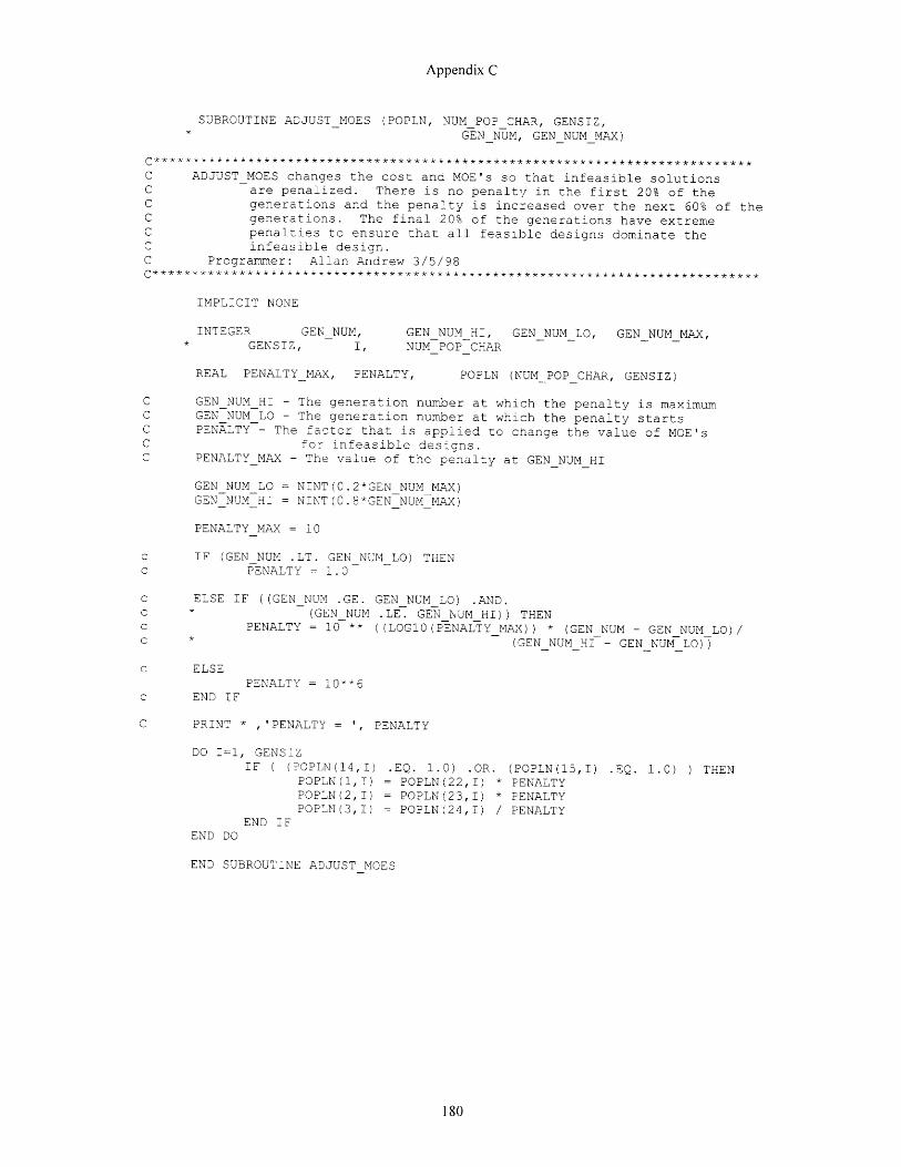
Appendix C
SUBROUTINE ADJUST_MOES (POPLN, NUM POP CHAR, GENSIZ,GENNUM, GENNUMMAX)
C*********************************
C ADJUST_MOES changes the cost and MOE's so that infeasible solutionsC are penalized. There is no penalty in the first 20% of theC generations and the penalty is increased over the next 60% of theC generations. The final 20% of the generations have extremeC penalties to ensure that all feasible designs dominate theC infeasible design.C Programmer: Allan Andrew 3/5/98C* ********* *************************** *** * *** *** ww *** w**w** w
IMPLICIT NONE
INTEGER GEN NUM, GEN NUM HI, GEN NUM LO, GEN NUM MAX,GENSIZ, I, NUM POP CHAR
REAL PENALTY_MAX, PENALTY, POPLN (NUM POP CHAR, GENSIZ)
C GEN_NUM_HI - The generation number at which the penalty is maximumC GEN NUM LO - The generation number at which the penalty startsC PENALTY - The factor that is applied to change the value of MOE'sC for infeasible designs.C PENALTY_MAX - The value of the penalty at GEN NUM HI
GEN NUM LO = NINT(0.2*GEN NUM MAX)GEN NUM HI = NINT(0.8*GEN-NUM-MAX)
PENALTY MAX = 10
c IF (GEN NUM .LT. GEN NUM LO) THENc PENALTY = 1.0
c ELSE IF ((GEN NUM .GE. GEN NUM LO) .AND.c * (GEN NUM .LE. GEN NUM HI)) THENc PENALTY = 10 ** ((LOG10(PENALTY MAX)) * (GEN NUM - GEN NUM LO)/c * (GEN NUM HI - GEN NUM LO))
c ELSEPENALTY = 10**6
c END IF
C PRINT * ,'PENALTY = ', PENALTY
DO I=l, GENSIZIF ( (?OPLN(14,I) .EQ. 1.0) .OR. (POPLN(15,I) .EQ. 1.0) ) THEN
POPLN(1,I) = POPLN(22,I) * PENALTYPOPLN(2,I) = POPLN(23,I) * PENALTYPOPLN(3,I) = POPLN(24,I) / PENALTY
END IFEND DO
END SUBROUTINE ADJUST MOES
180
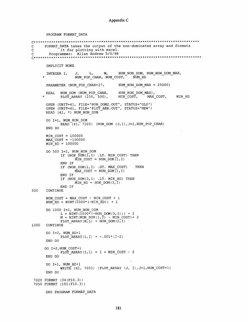
Appendix C
PROGRAM FORMAT DATA
C FORMATDATA takes the output of the non-dominated array and formats
C it for plotting with excel.
C Programmer: Allan Andrew 5/5/98
IMPLICIT NONE
INTEGER I, J, L, M, NUMNONDOM, NUMNON_DOM_MAX,NUMPOPCHAR, NUMCOST, NUMHD
PARAMETER (NUM POP CHAR=27, NUM NON DOM MAX = 25000)
REAL NON DOM (NUM POP CHAR, NUM NON DOM MAX),* PLOT ARRAY (100, 500), MIN-COST, MAX COST, MIN HD
OPEN (UNIT=41, FILE='NON DOM2.OUT', STATUS='OLD')OPEN (UNIT=61, FILE='PLOT ARR.OUT', STATUS='NEW')READ (41, *) NUM NON DOM
DO I=l, NUM NON DOMREAD (41, 7020) (NON DOM (J,I),J=1,NUM POP CHAR)
END DO
MIN COST = 100000MAX COST = -100000MIN HD = 100000
DO 500 I=1, NUM NON DOMIF (NON_DOM(1,I) .LT. MIN COST) THEN
MIN COST = NON DOM(1,I)END IFIF (NONDOM(1,I) .GT. MAX COST) THEN
MAX COST = NON DOM(1,I)END IFIF (NON DOM(3,I) .LT. MIN HD) THEN
MIN HD = NON DOM(3,I)END IF
500 CONTINUE
NUM COST = MAX COST - MIN COST + 1NUM HD = NINT(1000*(-MIN_ HD)) + 1
DO 1000 I=l, NUM NON DOML = NINT(1000*(-NON DOM(3,I))) + 2M = NINT(NON DOM(1,I) - MIN COST)+ 2PLOT ARRAY(M,L) = NON DOM(2,I)
1000 CONTINUE
DO I=2, NUM HD+1PLOT-ARRAY(1,I) = -.001*(I-2)
END DO
DO I=2,NUM COST+1PLOT ARRAY(I,1) = I + MIN COST - 2
END DO
DO I=l, NUM HD+1WRITE (61, 7050) (PLOTARRAY (J, I),J=1,NUM COST+1)
END DO
7020 FORMAT (34(F10.3))7050 FORMAT (101(F10.3))
END PROGRAM FORMAT DATA