News and Notes 4/8

• HW3 due date delayed to Tuesday 4/13– will hand out HW4 on 4/13 also

• Today: finish up NW economics• Tuesday 4/13

– another mandatory class exercise– topic: evolutionary game theory

Market Economiesand Networks

Networked LifeCSE 112

Spring 2004Prof. Michael Kearns

Market Economies• Suppose there are a bunch of different goods

– wheat, rice, paper, raccoon pelts, matches, grain alcohol,…– no differences or distinctions within a good: rice is rice

• We may all have different initial amounts or endowments– I might have 10 sacks of rice and two raccoon pelts– you might have 6 bushels of wheat, 2 boxes of matches– etc. etc. etc.

• Of course, we may want to exchange some of our goods– I can’t eat 10 sacks of rice, and I need matches to light a fire– it’s getting cold and you need raccoon mittens– etc. etc. etc.

• How should we engage in exchange?• What should be the rates of exchange?• These are among the oldest questions in economics

Cash and Prices• Suppose we introduce an abstract good called cash

– no inherent value– simply meant to facilitate trade, encode exchange rates

• And now suppose we introduce prices in cash– i.e. rates of exchange between each “real” good and

cash

• Then if we all believed in cash and the prices…– we might try to sell our initial endowments for cash– then use the cash to buy exactly what we most want

• But will there really be:– others who want to buy all of our endowments? (demand)– others who will be selling what we want? (supply)

Mathematical Economics• Have k abstract goods or commodities g1, g2, … , gk• Have n consumers or players• Each player has an initial endowment e = (e1,e2,…,ek)

> 0• Each consumer has their own utility function:

– assigns a personal valuation or utility to any amounts of the k goods

– e.g. if k = 4, U(x1,x2,x3,x4) = 0.2*x1 + 0.7*x2 + 0.3*x3 + 0.5*x4

– here g2 is my “favorite” good --- but it might be expensive– generally assume utility functions are insatiable

• always some bundle of goods you’d prefer more

– utility functions not necessarily linear, though

Market Equilibrium• Suppose we post prices p = (p1,p2,…,pk) for the k goods• Assume consumers are rational:

– they will attempt to sell their endowment e at the prices p (supply)– if successful, they will get cash e*p = e1*p1 + e2*p2 + … + ek*pk– with this cash, they will then attempt to purchase x = (x1,x2,…,xk)

that maximizes their utility U(x) subject to their budget (demand)– example:

• U(x1,x2,x3,x4) = 0.2*x1 + 0.7*x2 + 0.3*x3 + 0.5*x4• p = (1.0,0.35,0.15,2.0)• look at “bang for the buck” for each good i, wi/pi:

– g1: 0.2/1.0 = 0.2; g2: 0.7/0.35 = 2.0; g3: 0.3/0.15 = 2.0; g4: 0.5/2.0 = 0.25– so we will purchase as much of g2 and/or g3 as we can subject to budget

• Say that the prices p are an equilibrium if there are exactly enough goods to accomplish all supply and demand steps

• That is, supply exactly balances demand --- market clears

The Phone Call from Stockholm• Arrow and Debreu, 1954:

– There is always a set of equilibrium prices!– Both won Nobel prizes in Economics

• Intuition: suppose p is not an equilibrium– if there is excess demand for some good at p, raise its price– if there is excess supply for some good at p, lower its price– the “invisible hand” of the market

• The trickiness:– changing prices can radically alter consumer preferences

• not necessarily a gradual process; see “bang for the buck” argument

– everyone reacting/adjusting simultaneously– utility functions may be extremely complex

• May also have to specify “consumption plans”:– who buys exactly what from whom– example:

• A has Fruit Loops and Lucky Charms, but wants granola• B and C have only granola, both want either FL or LC (indifferent)• need to “coordinate” B and C to buy A’s FL and LC

Remarks• A&D 1954 a mathematical tour-de-force

– resolved and clarified a hundred of years of confusion– proof related to Nash’s; (n+1)-player game with “price player”

• Actual markets have been around for millennia– highly structured social systems– it’s the mathematical formalism and understanding that’s new

• Model abstracts away details of price adjustment process– modern financial markets– pre-currency bartering and trade– auctions– etc. etc. etc.

• Model can be augmented in various way:– labor as a commodity– firms producing goods from raw materials and labor– etc. etc. etc.

• “Efficient markets” ~ in equilibrium (at least at any given moment)

Network Economics• All of what we’ve said so far assumes:

– that anyone can trade (buy or sell) with anyone else– wheat bought from Nick is the same as wheat bought from Kilian– equivalently, exchange takes place on a complete network– global prices must emerge due to competition

• But there are many economic settings in which everyone is not free to trade with everyone else– geography:

• perishability: you buy groceries from local markets so it won’t spoil• labor: you purchases services from local residents

– legality:• if one were to purchase drugs, it is likely to be from an acquaintance (no

centralized market possible)• peer-to-peer music exchange

– politics:• there may be trade embargoes between nations

– regulations:• on Wall Street, certain transactions (within a firm) may be prohibited

Next Up

• A model of network economics• Analysis of our experiment• Network economics and preferential attachment

A Network Model of Market Economies

• Still begin with the same framework:– k goods or commodities– n consumers, each with their own endowments and utility functions

• But now assume an undirected network dictating exchange– each vertex is a consumer– edge between i and j means they are free to engage in trade– no edge between i and j: direct exchange is forbidden

• Note: can “encode” network in goods and utilities– for each raw good g and consumer i, introduce virtual good (g,i)– think of (g,i) as “good g when sold by consumer i”– consumer j will have

• zero utility for (g,i) if no edge between i and j• j’s original utility for g if there is an edge between i and j

Network Equilibrium

• Now prices are for each (g,i), not for just raw goods– permits the possibility of variation in price for raw goods– prices of (g,i) and (g,j) may differ– what would cause such variation at equilibrium?

• Each consumer must still behave rationally– attempt to sell all of initial endowment, but only to NW

neighbors– attempt to purchase goods maximizing utility within budget– will only purchase g from those neighbors with minimum price

for g

• Market equilibrium still always exists!– set of prices (and consumptions plans) such that:

• all initial endowments sold (no excess supply)• no consumer has money left over (no excess demand)

Our Experimental Network

• Four “island economies” --- groups A, B, C, D– can only engage in trade within group and with group E

• One economic “superpower” --- group E– can trade with anyone, including internally

• Group A: 6 buyers, 3 sellers (excess demand)• Group B: 3 buyers, 7 sellers (excess supply)• Group C: 5 buyers, 5 sellers (balanced)• Group D: 2 buyers, 5 sellers (excess supply)• Group E: 3 buyers, 3 sellers (internal balance

irrelevant)• Overall: 19 buyers, 23 sellers (excess supply)• What should happen at equilibrium?

The Theory Says…

• At equilibrium:– group E buyers join groups B and D (excess supply)– create merged economy of B, D (all parties) and E’s buyers– group E sellers join groups A (excess demand)– group C remains isolated, only trades internally– price computations:

• B-D-Ebuyers: cash/goods = 8/12 ~ 0.67• A-Esellers: cash/goods = 6/6 = 1.0• C: cash/goods = 5/5 = 1.0

– market incentive for E players to equalize opportunity– but price variation remains

D

C

B

E

A

sellers in bluebuyers in redignore edge color

the exchange subgraph at equilibrium

yellow: not competitive, unused

black: competitive, used

dashed: competitive, unused

0.67

1.00 1.00

What Actually Happened?

CSE112 Perpetrators:• colluded to inflate profits of Esell3 and Abuy5• $0 for 1, $1 for 0 transactions• agreed to split any prizes• we’ll come back to their fate

Esell3 Abuy2Asell1 Abuy5

Some Analysis• Market clearance:

– 18.56 dollars spent (out of 19)– 21.34 wheat sold (out of 23)

• Group A: 6 buyers, 3 sellers (excess demand)– average buyer price: 1.14; 1.23 excluding perp Abuy5– average seller price: 0.72; 1.13 excluding perp Asell1– versus 1.00 equilibrium

• Group B: 3 buyers, 7 sellers (excess supply)– average buyer price: 0.5, average seller price: 0.59– versus 0.67 equilibrium

• Group C: 5 buyers, 5 sellers (balanced)– average buyer price: 1.10, average seller price: 1.10– versus 1.00 equilibrium

• Group D: 2 buyers, 5 sellers (excess supply)– average buyer price: 0.65, average seller price: 0.71– versus 0.67 equilibrium

• Group E: 3 buyers, 3 sellers (internal balance irrelevant)– average buyer price: 0.72 (0.67 equilibrium)– average seller price: 1.47; 1.21 excluding perp Esell3 (1.00

equilibrium)• Qualitative agreement with equilibrium; higher prices overall

Prizes: $10 Each• Must have cleared (unloaded all of endowment)• Lowest avg prices for a buyer compared to equilibrium

– Bbuy1 (Eric Pierce): 0.38, vs 0.67 equilibrium (0.29 differential) – Abuy5 (Chenxi Jiao): 0.50, vs. 1.00 equilibrium (0.50

differential)

• Highest avg prices for a seller compared to equilibrium– Esell2 (Sarah Dong): 1.35, vs. 1.00 equilibrium (0.35

differential)– Esell3 (Scott Brown): 2.00, vs. 1.00 equilibrium (1.00

differential)

• Congratulations! • The SEC may be contacting some of you.

Markets on Natural Networks

• NW for class experiment highly artificial– very regular and simple structure– facilitated an easy experiment

• What happens on the NW types from SNT?– e.g. Erdos-Renyi, model, preferential attachment,…– we’ll take a quick look at preferential attachment– will have only buyers ($1) and sellers (1 wheat)– introduce a bipartite version of pref. att.

• Some personal comments on:– serving up only the freshest fare – the research-teaching-research cycle– MK talk tomorrow at CMU; (optional) paper on web site

A Preferential Attachment Modelfor Buyer-Seller Networks

• Probabilistically generates a bipartite graph• Buyers and sellers added in pairs at each time step• All edges between buyers and sellers• Each new party will have links back to extant graph

– note: generates bipartite trees – larger generates cyclical graphs

• Distribution of new buyer’s links:– with prob. 1 – : extant seller chosen w.r.t. preferential

attachment– with prob. : extant seller chosen uniformly at random– is pure pref. att.; is “like” Erdos-Renyi model

• So () characterizes distribution of generative model

A Sample Network and Equilibrium

• Solid edges:– exchange at equilibrium

• Dashed edges:– competitive but unused

• Dotted edges:– non-competitive prices

• Note price variation– 0.33 to 2.00

• Degree alone does not determine price!– e.g. B2 vs. B11– e.g. S5 vs. S14

Basic Theory

Statistics of the Network

• Can generate standard range of degree distributions• Define

– varies from (to

• Theorem: in the () model, for x = o(n^(1/)), the fraction of sellers at time n with degree > x is (x^()).– closely follows standard techniques– yields cumulative distribution (x^(-2))– as , tails become lighter; exponential decay at

Economics of the Network• Now not just interested in structural

properties of NW• Examine the properties of global

(equilibrium) computation• A useful monotonicity lemma:

– take a subgraph with a buyer (respectively, seller) frontier

– let p be the global equilibrium price of some good in this subgraph

– let p’ be its equilibrium price when computed just on the subgraph

– then p’ > p (respectively, p’ < p)• For example, seller degree is an

upper bound on seller wealth• This lemma has algorithmic

applications– compute controlled, local

approximations to global equilibrium prices

– how well will this work?

Economics of the Network• Theorem (Wealth Distribution): For w = o(n^()), the

fraction of sellers with wealth > w is O(w^(-)).– no corresponding lower bound yet– power laws seen empirically– not explained by degree distribution!

• Theorem (Price Variation): If (e.g.) (pure pref. att.), then (max price)/(min price) = (n^(2/))– = (n) for – = (n^(2/3)) for – variation generally scaling as a root of population size

Simulation Studies

Model: ()n = 250average of 25 trials

degree

wealth

Degree and Wealth Distributions

Power law wealth distribution at (rational) economic equilibrium

Degree and Wealth Distribution versus

Model: ()n = 250average of 25 trials

Increased lightens wealth tail, separates wealth and degree

Price Variation vs. NW Size &

Model: (varying)average of 25 trials

Power of network size (matches theory); decreasing with

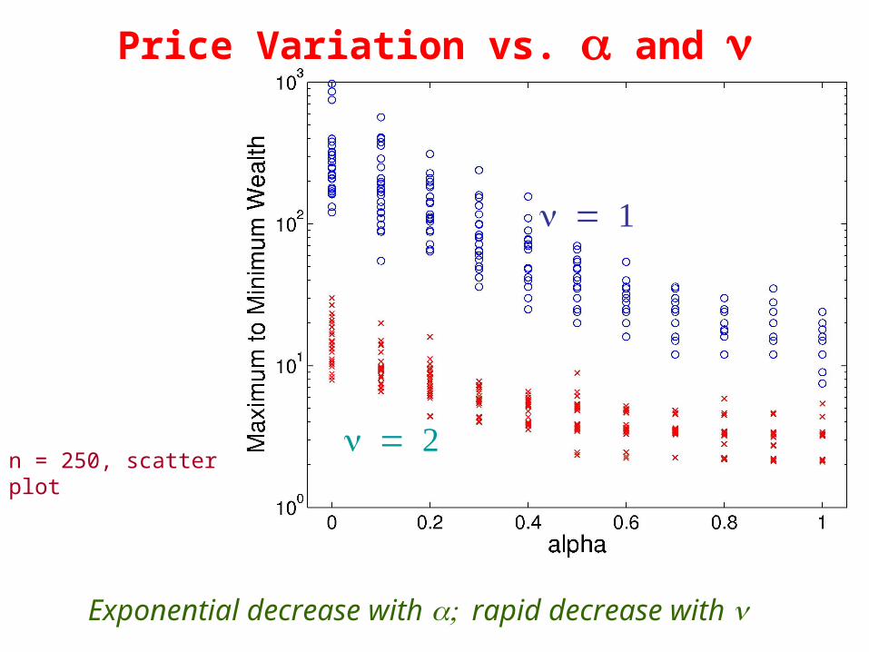
Price Variation vs. and

n = 250, scatter plot

Exponential decrease with rapid decrease with

Quality of Local Approximations

Model: ()n = 50 to 250 (five plots)each plot averages 5 trials

Very good approximations in small neighborhoodsError decays exponentially with k

Quality of Local Approximation II

Model: ()n = 50 to 250 (five plots)each plot averages 5 trials

Very mild dependence on n (Chung & Lu on loglog(n) core)k = 5 gives exact solution; k = 3 is 60% faster (n = 250)