Nonparametric StatisticsRelax Normality

Radu T. Trımbitas

May 19, 2016

1 Introduction

Introduction

• The term nonparametric statistics has no standard definition that is agreedon by all statisticians.

• Parametric methods – those that apply to problems where the distribu-tion(s) from which the sample(s) is (are) taken is (are) specified exceptfor the values of a finite number of parameters.

• Nonparametric methods apply in all other instances.

– The one-sample t test applies when the population is normally dis-tributed with unknown mean and variance. Because the distribu-tion from which the sample is taken is specified except for the valuesof two parameters, µ and σ2, the t test is a parametric procedure.

– Suppose that independent samples are taken from two populationsand we wish to test the hypothesis that the two population distri-butions are identical but of unspecified form. In this case, the dis-tribution is unspecified, and the hypothesis must be tested by usingnonparametric methods.

• Valid employment of some of the parametric methods presented in pre-ceding lectures requires that certain distributional assumptions are atleast approximately met. Even if all assumptions are met, research hasshown that nonparametric statistical tests are almost as capable of detect-ing differences among populations as the applicable parametric methods.They may be, and often are, more powerful in detecting population dif-ferences when the assumptions are not satisfied.

1

2 A General Two-Sample Shift Model

A General Two-Sample Shift Model

• Test wether two populations have the same distribution

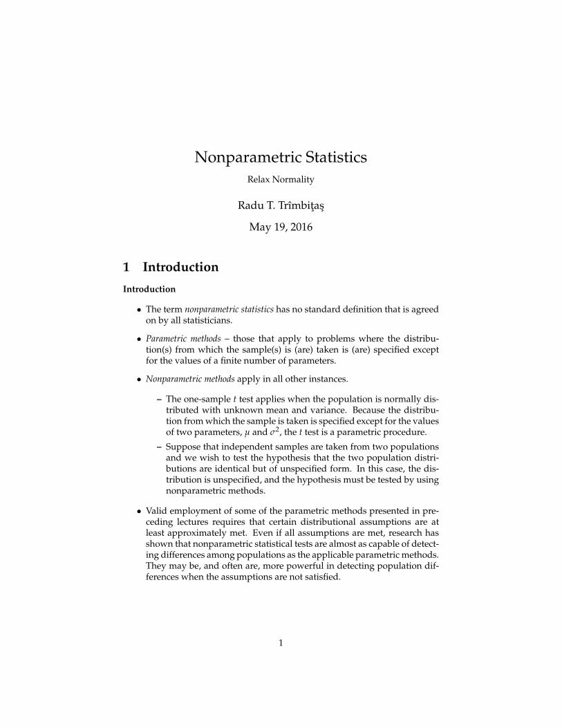
• Independent random samples X1, X2, . . . , Xn1 ∼ N(µX , σ2) and Y1, Y2,. . . , Yn2 ∼ N(µY, σ2); the experimenter may wish to test H0 : µX − µY = 0versus Ha : µX − µY < 0. If H0 is true, the population distributions areidentical. If Ha is true, then µY > µX and the distributions of X1 andY1 are the same, except that the location parameter (µY) for Y1 is largerthan the location parameter (µX) for X1. Hence, the distribution of Y1 isshifted to the right of the distribution of X1 (see Figure 1).

• This is an example of a two-sample parametric shift (or location) model.The model is parametric because the distributions are specified (normal)except for the values of the parameters µX , µY, and σ2. The amount thatthe distribution of Y1 is shifted to the right of the distribution of X1 isµY − µX (see Figure 1).

• We define a shift model that applies for any distribution, normal or oth-erwise.

• Let X1, X2, . . . , Xn1 be a random sample from a population with distri-bution function F(x) and let Y1, Y2, . . . , Yn2 be a random sample from apopulation with distribution function G(y). If we wish to test whetherthe two populations have the same distribution—that is, H0 : F(z) =G(z) versus Ha : F(z) 6= G(z), with the actual form of F(z) and G(z)unspecified—a nonparametric method is required.

• Notice that Ha is a very broad hypothesis.

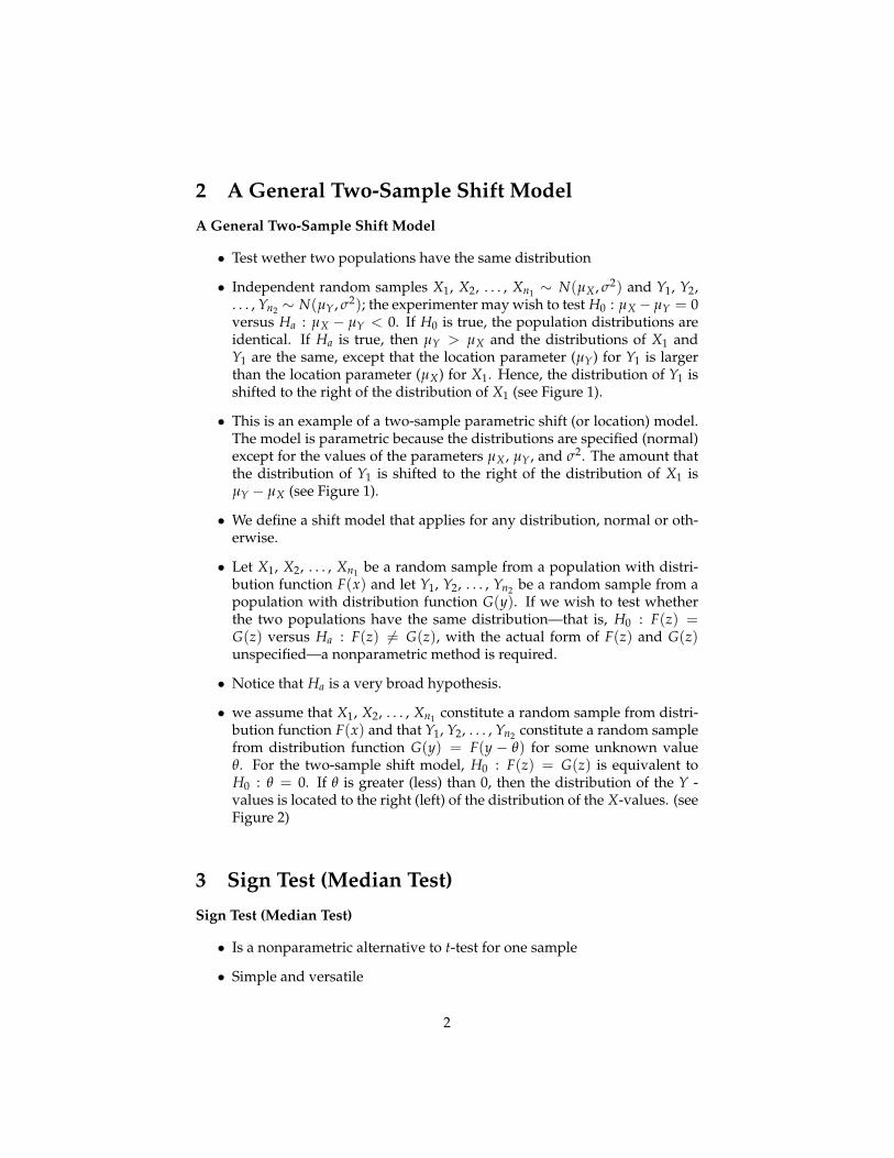
• we assume that X1, X2, . . . , Xn1 constitute a random sample from distri-bution function F(x) and that Y1, Y2, . . . , Yn2 constitute a random samplefrom distribution function G(y) = F(y − θ) for some unknown valueθ. For the two-sample shift model, H0 : F(z) = G(z) is equivalent toH0 : θ = 0. If θ is greater (less) than 0, then the distribution of the Y -values is located to the right (left) of the distribution of the X-values. (seeFigure 2)

3 Sign Test (Median Test)

Sign Test (Median Test)

• Is a nonparametric alternative to t-test for one sample

• Simple and versatile

2

Figure 1: Two normal distributions with same variances and different means

Figure 2: Two probability densities, one shifted with θ with resppect to theother

3

• Hypotheses H0 : m = m0 (median) with respect to usual alternatives

• The data are converted to and signs according to whether each data valueis more or less than m0. A plus sign will be assigned to each larger thanm0, a minus sign to each smaller than m0, and a zero to those equal to m0.The sign test uses only the plus and minus signs; the zeros are discarded.

• Test statistics M = min(n(+), n(−)), where n(+) is the number of +signs. Distribution of M ∼ b(n, 1/2).

• Normal approximation

Z =M− n/2√

n2

.

Example 1. The following data give temperature (in ◦C) for 20 days: 22 18 17 1613 20 19 21 20 16 14 17 21 21 17 17 17 22 22 21. Test if the median is m = 19.

Solution. See nonpar/ex15_0.pdf

4 The Sign Test for a Matched-Pairs Experiment

The Sign Test for a Matched-Pairs Experiment

• n pairs of observations of the form (Xi, Yi); H0 : X and Y have the samecontinuous distributions; Ha : the distributions differ in location.

• Let Di = Xi −Yi. H0 is true =⇒ P(Di > 0) = P(Di < 0) = 1/2

• Let M denote the total number of positive (or negative) differences. Thenif the variables Xi and Yi have the same distribution, M has a binomialdistribution with p = 1/2, and the rejection region for a test based on Mcan be obtained by using the binomial probability distribution.

• Problem that may arise: observations associated with one or more pairsmay be equal and therefore may result in ties. When this situation occurs,delete the tied pairs and reduce n, the total number of pairs.

Sign Test SummaryThe Sign Test for a Matched-Pairs ExperimentLet p = P(X > Y).

Null hypothesis: H0 : p = 1/2.

Alternative hypothesis: Ha : p > 1/2 or (p < 1/2 or p 6= 1/2).

Test statistic: M = card{Di = Xi −Yi > 0 : i = 1, . . . , n}.

Rejection region: • For Ha : p > 1/2, reject H0 for the largest values of M;

4

Day A B1 172 2012 165 1793 206 1594 184 1925 174 1776 142 1707 190 1828 169 1799 161 169

10 200 210

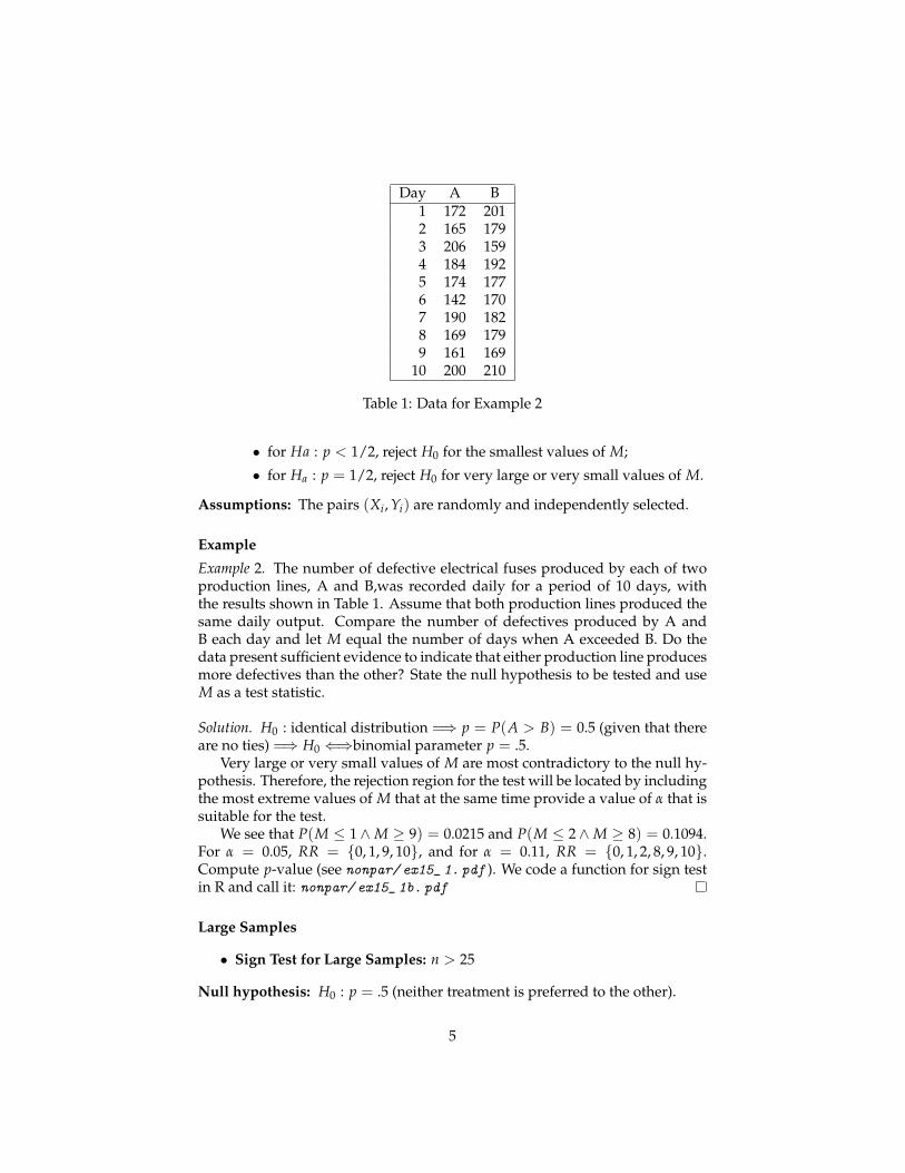
Table 1: Data for Example 2

• for Ha : p < 1/2, reject H0 for the smallest values of M;

• for Ha : p = 1/2, reject H0 for very large or very small values of M.

Assumptions: The pairs (Xi, Yi) are randomly and independently selected.

Example

Example 2. The number of defective electrical fuses produced by each of twoproduction lines, A and B,was recorded daily for a period of 10 days, withthe results shown in Table 1. Assume that both production lines produced thesame daily output. Compare the number of defectives produced by A andB each day and let M equal the number of days when A exceeded B. Do thedata present sufficient evidence to indicate that either production line producesmore defectives than the other? State the null hypothesis to be tested and useM as a test statistic.

Solution. H0 : identical distribution =⇒ p = P(A > B) = 0.5 (given that thereare no ties) =⇒ H0 ⇐⇒binomial parameter p = .5.

Very large or very small values of M are most contradictory to the null hy-pothesis. Therefore, the rejection region for the test will be located by includingthe most extreme values of M that at the same time provide a value of α that issuitable for the test.

We see that P(M ≤ 1 ∧M ≥ 9) = 0.0215 and P(M ≤ 2 ∧M ≥ 8) = 0.1094.For α = 0.05, RR = {0, 1, 9, 10}, and for α = 0.11, RR = {0, 1, 2, 8, 9, 10}.Compute p-value (see nonpar/ ex15_ 1. pdf ). We code a function for sign testin R and call it: nonpar/ ex15_ 1b. pdf

Large Samples

• Sign Test for Large Samples: n > 25

Null hypothesis: H0 : p = .5 (neither treatment is preferred to the other).

5

Alternative hypothesis: Ha : p = .5 for a two-tailed test (Note: We use thetwo-tailed test for an example. Many analyses require a one-tailed test.)

Test statistic:Z =

M− n/212√

n.

Rejection region: Reject H0 if z ≥ zα/2 or if z ≤ −zα/2, where zα/2 is thequantile of order α/2 for standard normal distribution.

ExampleThe data in the file chickenembrios.txt are a subset of the data obtained

by Oppenheim (1968) in an experiment investigating light responsivity in chickembryos. The subjects were white leghorn chick embryos, and the behavioralresponse measured in the investigation was beak-clapping (i.e., the rapid open-ing and closing of the beak that occurs during the latter one-third of incubationin chick embryos). (Gottlieb (1965) had previously shown that changes in therate of beak-clapping constituted a sensitive indicator of auditory responsive-ness in chick embryos.)

The embryos were placed in a dark chamber 30 min before the initiation oftesting. Then ten 1-min readings were taken in the dark, and at the end of this10-min period, a single reading was obtained for a 1-min period of illumina-tion.

File chickenembrios.txt gives the average number of claps per minuteduring the dark period (XD) and the corresponding rate during the period ofillumination (YL) for 25 chick embryos. nonpar/ chikenEmbriosls. pdf

Comments

• Suppose that the paired differences are normally distributed with a com-mon variance σ2. Will the sign test detect a shift in location of the twopopulations as effectively as the Student’s t test?

• Intuitively: no. This is correct because the Student’s t test uses moreinformation: sign +magnitude of differences for more accurate meansand variances.

• Thus, we might say that the sign test is not as “efficient” as the Student’st test; but this statement is meaningful only if the differences in pairedobservations are normally distributed with a common variance σ2

D.

• The sign test might be more efficient when these assumptions are notsatisfied.

6

5 The Wilcoxon Signed-Rank Test for a Matched-Pairs Experiment

The Wilcoxon Signed-Rank Test for a Matched-Pairs Experiment

• We have n paired observations (Xi, Yi) and Di = Xi −Yi.

• H0: the X’s and the Y’s have the same distribution versus the alternativethat the distributions differ in location. Under the null hypothesis of nodifference in the distributions of the X’s and Y’s, you would expect (onthe average) half of the differences in pairs to be negative and half to bepositive.

• That is, the expected number of negative differences between pairs is n/2(where n is the number of pairs). Further, it would follow that positiveand negative differences of equal absolute magnitude should occur withequal probability.

• If we were to order the differences according to their absolute values andrank them from smallest to largest, the expected rank sums for the nega-tive and positive differences would be equal.

• Sizable differences in the sums of the ranks assigned to the positive andnegative differences would provide evidence to indicate a shift in loca-tion for the two distributions.

• To carry out the Wilcoxon test:

1. We calculate the differences (Di) for each of the n pairs. Differencesequal to zero are eliminated, and the number of pairs, n, is reducedaccordingly.

2. We rank the absolute values of the differences, assigning a 1 to thesmallest, a 2 to the second smallest, and so on. Ties: If two or moreabsolute differences are tied for the same rank, then the average ofthe ranks that would have been assigned to these differences is as-signed to each member of the tied group. For example, if two ab-solute differences are tied for ranks 3 and 4, then each receives rank3.5, and the next highest absolute difference is assigned rank 5.

3. Then we calculate the sum of the ranks (rank sum) for the nega-tive differences and also calculate the rank sum for the positive dif-ferences. For a two-tailed test, we use T, the smaller of these twoquantities, as a test statistic to test the null hypothesis that the twopopulation relative frequency histograms are identical. The smallerthe value of T is, the greater will be the weight of evidence favor-ing rejection of the null hypothesis. Hence, we will reject the nullhypothesis if T is less than or equal to some value, say, T0.

7

4. To detect the one-sided alternative, that the distribution of the X’sis shifted to the right of that of the Y’s, we use the rank sum T− ofthe negative differences, and we reject the null hypothesis for smallvalues of T−, say, T− ≤ T0. If we wish to detect a shift of the distri-bution of the Y’s to the right of the X’s,we use the rank sum T+ ofthe positive differences as a test statistic, and we reject small valuesof T+, say, T+ ≤ T0.

• The probability that T is less than or equal to some value T0 has beencalculated for a combination of sample sizes and values of T0. Theseprobabilities are tabulated and can be used to find the rejection region forthe test based on T.

• The R functions dsignrank, psignrank, qsignrank, rsignrank are den-sity, distribution function, quantile function and random generation, re-spectively, for the distribution of the Wilcoxon Signed Rank statistic ob-tained from a sample with size n.

SummaryWilcoxon Signed-Rank Test for a Matched-Pairs Experiment

H0 : The population distributions for the X’s and Y’s are identical.

Ha : (1) The two population distributions differ in location (two-tailed), or (2)the population relative frequency distribution for the X’s is shifted to theright of that for the Y ’s (one-tailed).

Test statistic 1. For a two-tailed test, use T = min(T+, T−), where T+ =sum of the ranks of the positive differences and T− = sum of theranks of the negative differences.

2. For a one-tailed test (to detect the one-tailed alternative just given),use the rank sum T− of the negative differences. To detect a shift ofthe distribution of the Y’s to the right of the distribution of the X’s,use the rank sum T+, the sum of the ranks of the positive differences,and reject H0 if T+ ≤ T0.

Rejection region: 1. For a two-tailed test, reject H0 if T ≤ T0, where T0 isthe critical value for the two-sided test

2. For a one-tailed test (as described earlier), reject H0 if T− ≤ T0,where T0 is the critical value for the one-sided test.

Example

Example 3. Due to oven-to-oven variation, a matched-pairs experiment wasused to test for differences in cakes prepared using mix A and mix B. Twocakes, one prepared using each mix, were baked in each of six different ovens(a total of 12 cakes). Test the hypothesis that there is no difference in population

8

Difference Absolute Rank ofA B A− B Difference Absolute Difference

.135 .129 .006 .006 3

.102 .120 −.018 .018 5

.108 .112 −.004 .004 1.5

.141 .152 −.011 .011 4

.131 .135 −.004 .004 1.5

.144 .163 −.019 .019 6

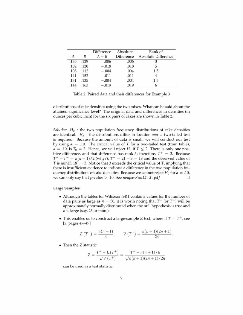
Table 2: Paired data and their differences for Example 3

distributions of cake densities using the two mixes. What can be said about theattained significance level? The original data and differences in densities (inounces per cubic inch) for the six pairs of cakes are shown in Table 2.

Solution. H0 : the two population frequency distributions of cake densitiesare identical. Ha : the distributions differ in location =⇒ a two-tailed testis required. Because the amount of data is small, we will conduct our testby using α = .10. The critical value of T for a two-tailed test (from table),α = .10, is T0 = 2. Hence, we will reject H0 if T ≤ 2. There is only one pos-itive difference, and that difference has rank 3; therefore, T+ = 3. BecauseT+ + T− = n(n + 1)/2 (why?), T− = 21− 3 = 18 and the observed value ofT is min(3, 18) = 3. Notice that 3 exceeds the critical value of T, implying thatthere is insufficient evidence to indicate a difference in the two population fre-quency distributions of cake densities. Because we cannot reject H0 for α = .10,we can only say that p-value > .10. See nonpar/ ex15_ 3. pdf

Large Samples

• Although the tables for Wilcoxon SRT contains values for the number ofdata pairs as large as n = 50, it is worth noting that T+ (or T−) will beapproximately normally distributed when the null hypothesis is true andn is large (say, 25 or more).

• This enables us to construct a large-sample Z test, where if T = T+, see[2, pages 47–49]

E(T+)=

n(n + 1)4

, V(T+)=

n(n + 1)(2n + 1)24

.

• Then the Z statistic

Z =T+ − E (T+)√

V (T+)=

T+ − n(n + 1)/4√n(n + 1)(2n + 1)/24

can be used as a test statistic.

9

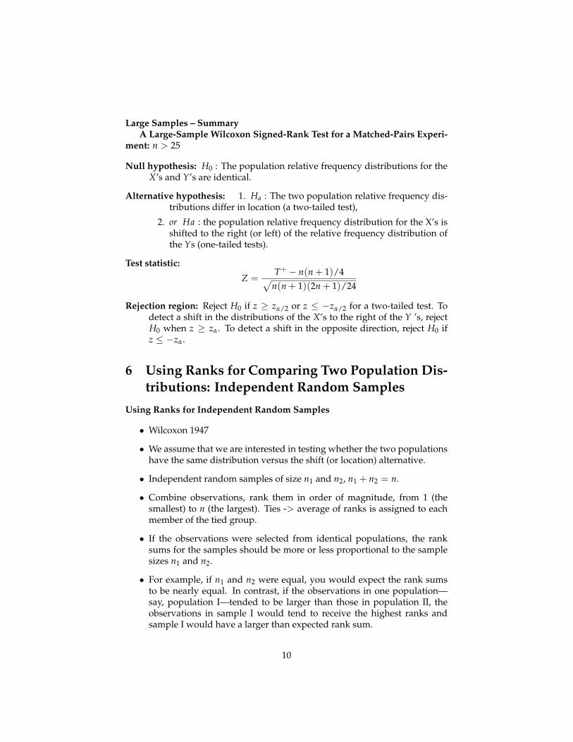
Large Samples – SummaryA Large-Sample Wilcoxon Signed-Rank Test for a Matched-Pairs Experi-

ment: n > 25

Null hypothesis: H0 : The population relative frequency distributions for theX’s and Y’s are identical.

Alternative hypothesis: 1. Ha : The two population relative frequency dis-tributions differ in location (a two-tailed test),

2. or Ha : the population relative frequency distribution for the X’s isshifted to the right (or left) of the relative frequency distribution ofthe Ys (one-tailed tests).

Test statistic:

Z =T+ − n(n + 1)/4√

n(n + 1)(2n + 1)/24

Rejection region: Reject H0 if z ≥ zα/2 or z ≤ −zα/2 for a two-tailed test. Todetect a shift in the distributions of the X’s to the right of the Y ’s, rejectH0 when z ≥ zα. To detect a shift in the opposite direction, reject H0 ifz ≤ −zα.

6 Using Ranks for Comparing Two Population Dis-tributions: Independent Random Samples

Using Ranks for Independent Random Samples

• Wilcoxon 1947

• We assume that we are interested in testing whether the two populationshave the same distribution versus the shift (or location) alternative.

• Independent random samples of size n1 and n2, n1 + n2 = n.

• Combine observations, rank them in order of magnitude, from 1 (thesmallest) to n (the largest). Ties -> average of ranks is assigned to eachmember of the tied group.

• If the observations were selected from identical populations, the ranksums for the samples should be more or less proportional to the samplesizes n1 and n2.

• For example, if n1 and n2 were equal, you would expect the rank sumsto be nearly equal. In contrast, if the observations in one population—say, population I—tended to be larger than those in population II, theobservations in sample I would tend to receive the highest ranks andsample I would have a larger than expected rank sum.

10

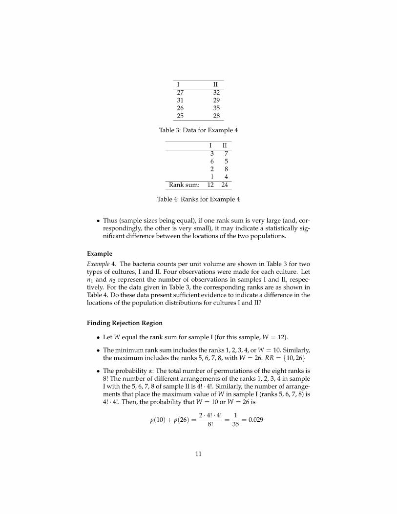
I II27 3231 2926 3525 28

Table 3: Data for Example 4

I II3 76 52 81 4

Rank sum: 12 24

Table 4: Ranks for Example 4

• Thus (sample sizes being equal), if one rank sum is very large (and, cor-respondingly, the other is very small), it may indicate a statistically sig-nificant difference between the locations of the two populations.

Example

Example 4. The bacteria counts per unit volume are shown in Table 3 for twotypes of cultures, I and II. Four observations were made for each culture. Letn1 and n2 represent the number of observations in samples I and II, respec-tively. For the data given in Table 3, the corresponding ranks are as shown inTable 4. Do these data present sufficient evidence to indicate a difference in thelocations of the population distributions for cultures I and II?

Finding Rejection Region

• Let W equal the rank sum for sample I (for this sample, W = 12).

• The minimum rank sum includes the ranks 1, 2, 3, 4, or W = 10. Similarly,the maximum includes the ranks 5, 6, 7, 8, with W = 26. RR = {10, 26}

• The probability α: The total number of permutations of the eight ranks is8! The number of different arrangements of the ranks 1, 2, 3, 4 in sampleI with the 5, 6, 7, 8 of sample II is 4! · 4!. Similarly, the number of arrange-ments that place the maximum value of W in sample I (ranks 5, 6, 7, 8) is4! · 4!. Then, the probability that W = 10 or W = 26 is

p(10) + p(26) =2 · 4! · 4!

8!=

135

= 0.029

11

• If this value of α is too small, the rejection region can be enlarged to in-clude the next smallest and next largest rank sums, W = 11 and W = 25.The rank sum W = 11 includes the ranks 1, 2, 3, 5, and

p(11) =4! · 4!

8!=

170

Similarly,

p(25) =170

.

Then,

α = p(10) + p(11) + p(25) + p(26) =2

35= 0.057.

• Expansion of the rejection region to include 12 and 24 substantially in-creases the value of α. The set of sample points giving a rank of 12 in-cludes all sample points associated with rankings of (1, 2, 3, 6) and (1, 2,4, 5). Thus,

p(12) =2 · 4! · 4!

8!=

135

and

α = p(10) + p(11) + p(12) + p(24) + p(25) + p(26)

=1

70+

170

+135

+1

35+

170

+1

70=

435

= 0.114

This value of α might be considered too large for practical purposes.Hence, we are better satisfied with the rejection region W = 10, 11, 25,and 26. The rank sum for the sample, W = 12, does not fall in this pre-ferred rejection region, so we do not have sufficient evidence to reject thehypothesis that the population distributions of bacteria counts for thetwo cultures are identical.

7 The Mann–Whitney U Test

The Mann-Whitney U Test - Logic

• The Mann–Whitney statistic U is obtained by ordering all n1 + n2 ob-servations according to their magnitude and counting the number of ob-servations in sample I that precede each observation in sample II. Thestatistic U is the sum of these counts.

• We denote the observations in sample I as x1, x2, . . . , xn1 and the obser-vations in sample II as y1, y2, . . . , yn2 . For example, the eight orderedobservations of Example 4 are

25 26 27 28 29 31 32 35x(1) x(2) x(3) y(1) y(2) x(4) y(3) y(4)

12

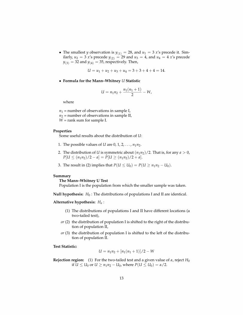
• The smallest y observation is y(1) = 28, and u1 = 3 x’s precede it. Sim-ilarly, u2 = 3 x’s precede y(2) = 29 and u3 = 4, and u4 = 4 x’s precedey(3) = 32 and y(4) = 35, respectively. Then,

U = u1 + u2 + u3 + u4 = 3 + 3 + 4 + 4 = 14.

• Formula for the Mann–Whitney U Statistic

U = n1n2 +n1(n1 + 1)

2−W,

where

n1 = number of observations in sample I,n2 = number of observations in sample II,W = rank sum for sample I.

PropertiesSome useful results about the distribution of U:

1. The possible values of U are 0, 1, 2, . . . , n1n2.

2. The distribution of U is symmetric about (n1n2)/2. That is, for any a > 0,P[U ≤ (n1n2)/2− a] = P[U ≥ (n1n2)/2 + a].

3. The result in (2) implies that P(U ≤ U0) = P(U ≥ n1n2 −U0).

SummaryThe Mann–Whitney U TestPopulation I is the population from which the smaller sample was taken.

Null hypothesis: H0 : The distributions of populations I and II are identical.

Alternative hypothesis: Ha :

(1) The distributions of populations I and II have different locations (atwo-tailed test),

or (2) the distribution of population I is shifted to the right of the distribu-tion of population II,

or (3) the distribution of population I is shifted to the left of the distribu-tion of population II.

Test Statistic:U = n1n2 + [n1(n1 + 1)]/2−W

Rejection region: (1) For the two-tailed test and a given value of α, reject H0if U ≤ U0 or U ≥ n1n2 −U0, where P(U ≤ U0) = α/2.

13

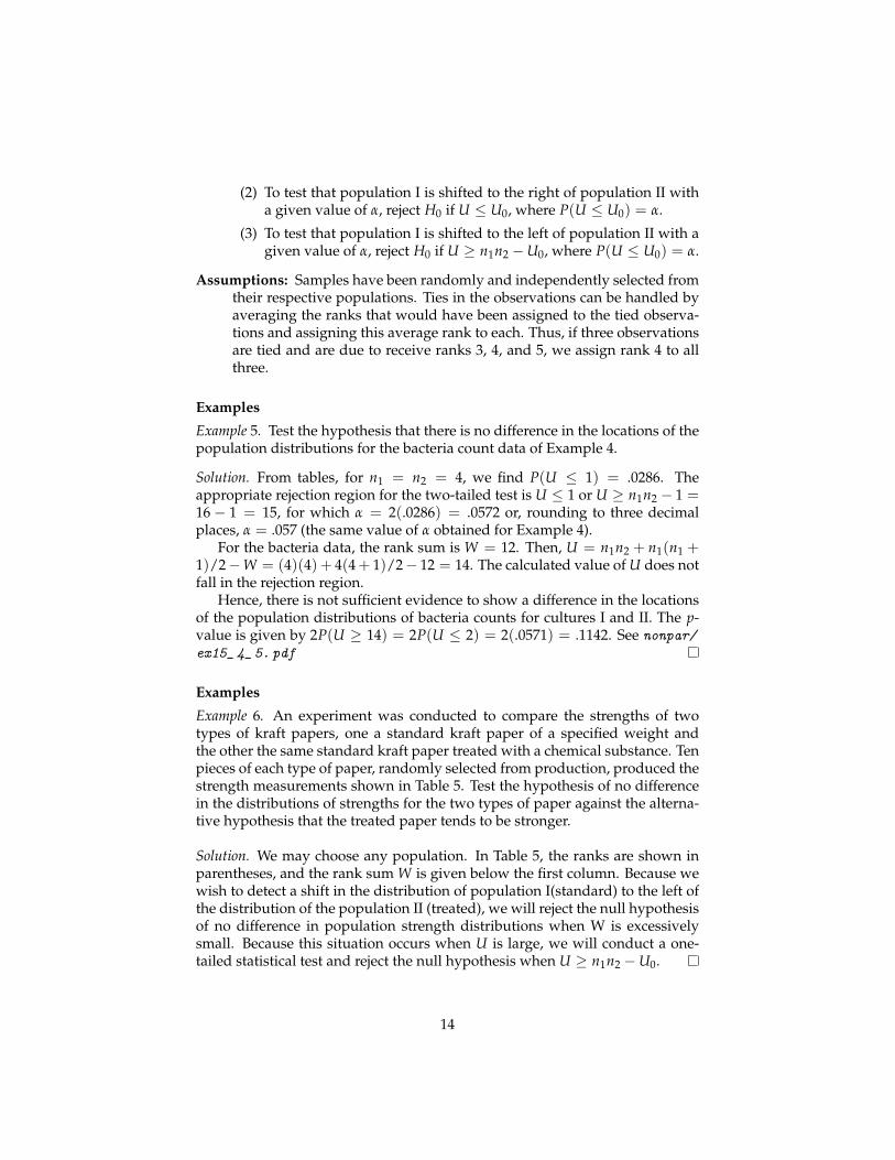
(2) To test that population I is shifted to the right of population II witha given value of α, reject H0 if U ≤ U0, where P(U ≤ U0) = α.

(3) To test that population I is shifted to the left of population II with agiven value of α, reject H0 if U ≥ n1n2 −U0, where P(U ≤ U0) = α.

Assumptions: Samples have been randomly and independently selected fromtheir respective populations. Ties in the observations can be handled byaveraging the ranks that would have been assigned to the tied observa-tions and assigning this average rank to each. Thus, if three observationsare tied and are due to receive ranks 3, 4, and 5, we assign rank 4 to allthree.

Examples

Example 5. Test the hypothesis that there is no difference in the locations of thepopulation distributions for the bacteria count data of Example 4.

Solution. From tables, for n1 = n2 = 4, we find P(U ≤ 1) = .0286. Theappropriate rejection region for the two-tailed test is U ≤ 1 or U ≥ n1n2 − 1 =16 − 1 = 15, for which α = 2(.0286) = .0572 or, rounding to three decimalplaces, α = .057 (the same value of α obtained for Example 4).

For the bacteria data, the rank sum is W = 12. Then, U = n1n2 + n1(n1 +1)/2−W = (4)(4) + 4(4+ 1)/2− 12 = 14. The calculated value of U does notfall in the rejection region.

Hence, there is not sufficient evidence to show a difference in the locationsof the population distributions of bacteria counts for cultures I and II. The p-value is given by 2P(U ≥ 14) = 2P(U ≤ 2) = 2(.0571) = .1142. See nonpar/

ex15_ 4_ 5. pdf

Examples

Example 6. An experiment was conducted to compare the strengths of twotypes of kraft papers, one a standard kraft paper of a specified weight andthe other the same standard kraft paper treated with a chemical substance. Tenpieces of each type of paper, randomly selected from production, produced thestrength measurements shown in Table 5. Test the hypothesis of no differencein the distributions of strengths for the two types of paper against the alterna-tive hypothesis that the treated paper tends to be stronger.

Solution. We may choose any population. In Table 5, the ranks are shown inparentheses, and the rank sum W is given below the first column. Because wewish to detect a shift in the distribution of population I(standard) to the left ofthe distribution of the population II (treated), we will reject the null hypothesisof no difference in population strength distributions when W is excessivelysmall. Because this situation occurs when U is large, we will conduct a one-tailed statistical test and reject the null hypothesis when U ≥ n1n2 −U0.

14

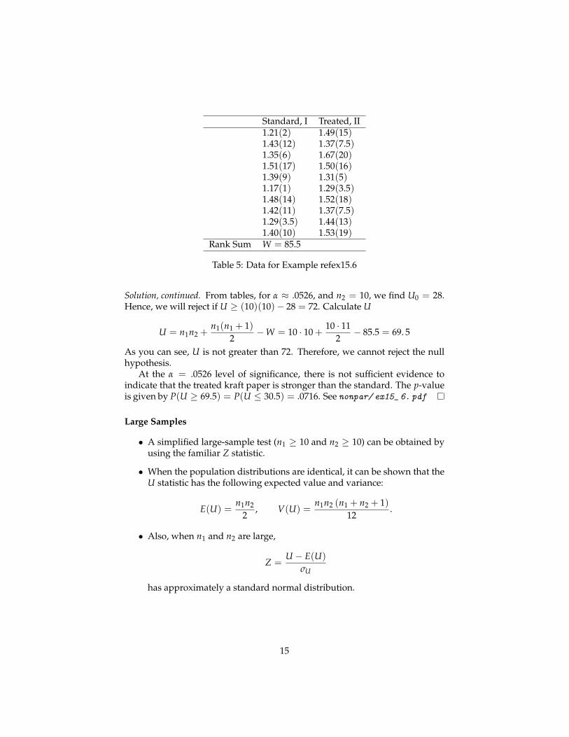
Standard, I Treated, II1.21(2) 1.49(15)1.43(12) 1.37(7.5)1.35(6) 1.67(20)1.51(17) 1.50(16)1.39(9) 1.31(5)1.17(1) 1.29(3.5)1.48(14) 1.52(18)1.42(11) 1.37(7.5)1.29(3.5) 1.44(13)1.40(10) 1.53(19)

Rank Sum W = 85.5

Table 5: Data for Example refex15.6

Solution, continued. From tables, for α ≈ .0526, and n2 = 10, we find U0 = 28.Hence, we will reject if U ≥ (10)(10)− 28 = 72. Calculate U

U = n1n2 +n1(n1 + 1)

2−W = 10 · 10 +

10 · 112− 85.5 = 69. 5

As you can see, U is not greater than 72. Therefore, we cannot reject the nullhypothesis.

At the α = .0526 level of significance, there is not sufficient evidence toindicate that the treated kraft paper is stronger than the standard. The p-valueis given by P(U ≥ 69.5) = P(U ≤ 30.5) = .0716. See nonpar/ ex15_ 6. pdf

Large Samples

• A simplified large-sample test (n1 ≥ 10 and n2 ≥ 10) can be obtained byusing the familiar Z statistic.

• When the population distributions are identical, it can be shown that theU statistic has the following expected value and variance:

E(U) =n1n2

2, V(U) =

n1n2 (n1 + n2 + 1)12

.

• Also, when n1 and n2 are large,

Z =U − E(U)

σU

has approximately a standard normal distribution.

15

Comments

• The Mann–Whitney U test and the equivalent Wilcoxon rank-sum test arenot very efficient because they do not appear to use all the information inthe sample. Actually, theoretical studies have shown that this is not thecase.

• Under the normality assumption, the two-sample t test and the Mann–Whitney U test test the same hypotheses: H0 : µ1 − µ2 = 0 versus Ha :µ1 − µ2 > 0.

• For a given α and β, the total sample size required for the t test is approx-imately .95 times the total sample size required for the Mann–WhitneyU.

• Thus, the nonparametric procedure is almost as good as the t test for thesituation in which the t test is optimal.

• For many nonnormal distributions, the nonparametric procedure requiresfewer observations than a corresponding parametric procedure wouldrequire to produce the same values of α and β.

8 The Kruskal–Wallis Test for the One-Way Layout

The Kruskal–Wallis Test

• We assume that independent random samples have been drawn from kpopulations that differ only in location, and we let ni, for i = 1, 2, . . . , k,represent the size of the sample drawn from the ith population.

• Combine all the n1 + n2 + · · ·+ nk = n observations and rank them from1 (the smallest) to n (the largest).

• Ties: if two or more observations are tied for the same rank, then theaverage of the ranks that would have been assigned to these observationsis assigned to each member of the tied group.

• Let Ri denote the sum of the ranks of the observations from population iand let Ri = Ri/ni denote the corresponding average of the ranks. If Requals the overall average of all of the ranks, consider the rank analogue ofSST, which is computed by using the ranks rather than the actual valuesof the measurements:

V =k

∑i=1

ni(

Ri − R)2 .

16

• If the null hypothesis is true and the populations do not differ in loca-tion, we would expect the Ri values to be approximately equal and theresulting value of V to be relatively small. If the alternative hypothe-sis is true, we would expect this to be exhibited in differences amongthe values of the Ri values, leading to a large value for V. Notice thatR = (∑n

k=1 k)/n = [n(n + 1)/2]/n = (n + 1)/2 and thus that

V =k

∑i=1

ni

(Ri −

n + 12

)2. (1)

• Instead of focusing on V, Kruskal and Wallis (1952) [3] considered thestatistic

H =12V

n(n + 1), (2)

which may be rewritten (homework)

H =12

n (n + 1)

k

∑i=1

R2i

ni− 3 (n + 1) . (3)

• As previously noted, the null hypothesis of equal locations is rejected infavor of the alternative that the populations differ in location if the valueof H is large. Thus, the corresponding α-level test calls for rejection of thenull hypothesis in favor of the alternative if H > h(α), where h(α) is suchthat, when H0 is true, P[H > h(α)] = α.

• If the underlying distributions are continuous and if there are no tiesamong the n observations, the null distribution of H can (tediously) befound by using the methods of Probability Theory. We can find the dis-tribution of H for any values of k and n1, n2, . . . , nk by calculating thevalue of H for each of the n! equally likely permutations of the ranks ofthe n observations. These calculations have been performed and tablesdeveloped for some relatively small values of k and for n1, n2, . . . , nk [2,Table A.12].

SummaryKruskal–Wallis Test Based on H for Comparing k Population Distribu-

tions

Null hypothesis: H0: The k population distributions are identical.

Alternative hypothesis: Ha: At least two of the population distributions differin location.

Test statistic:

H =12

n (n + 1)

k

∑i=1

R2i

ni− 3 (n + 1) .

17

Line 1 Line 2 Line 3Def R Def R Def R6 5 34 25 13 9.5

38 27 28 19 35 263 2 42 30 19 15

17 13 13 9.5 4 311 8 40 29 29 2030 21 31 22 0 115 11 9 7 7 616 12 32 23 33 2425 17 39 28 18 145 4 27 18 24 16

R1 = 120 R2 = 210.5 R3 = 134.5

Table 6: Data for Example 7

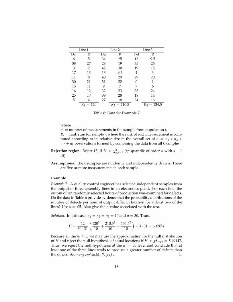
whereni = number of measurements in the sample from population i,Ri = rank sum for sample i, where the rank of each measurement is com-puted according to its relative size in the overall set of n = n1 + n2 +· · ·+ nk observations formed by combining the data from all k samples.

Rejection region: Reject H0 if H > χ2α,k−1 (χ2-quantile of order α with k − 1

df).

Assumptions: The k samples are randomly and independently drawn. Thereare five or more measurements in each sample.

Example

Example 7. A quality control engineer has selected independent samples fromthe output of three assembly lines in an electronics plant. For each line, theoutput of ten randomly selected hours of production was examined for defects.Do the data in Table 6 provide evidence that the probability distributions of thenumber of defects per hour of output differ in location for at least two of thelines? Use α = .05. Also give the p-value associated with the test.

Solution. In this case, n1 = n2 = n3 = 10 and n = 30. Thus,

H =12

30 · 31

(1202

10+

210.52

10+

134.52

10

)− 3 · 31 = 6. 097 4

Because all the ni ≥ 5, we may use the approximation for the null distributionof H and reject the null hypothesis of equal locations if H > χ2

0.05,2 = 5.99147.Thus, we reject the null hypothesis at the α = .05 level and conclude that atleast one of the three lines tends to produce a greater number of defects thanthe others. See nonpar/ ex15_ 7. pdf .

18

Remarks

• It can be shown that, if we wish to compare only k = 2 populations, theKruskal–Wallis test is equivalent to the Wilcoxon rank-sum two-sidedtest. If data are obtained from a one-way layout involving k > 2 pop-ulations but we wish to compare a particular pair of populations, theWilcoxon rank-sum test (or the equivalent Mann–Whitney U test) can beused for this purpose.

• Notice that the analysis based on the Kruskal–Wallis H statistic does notrequire knowledge of the actual values of the observations. We need onlyknow the ranks of the observations to complete the analysis.

9 The Friedman Test for Randomized Block Designs

The Friedman Test for Randomized Block Designs

• Milton Friedman - winner of Nobel Prize for Economy, 1937

• After the data from a randomized block design are obtained, within eachblock the observed values of the responses to each of the k treatments areranked from 1 (the smallest in the block) to k (the largest in the block).

• If two or more observations in the same block are tied for the same rank,then the average of the ranks that would have been assigned to theseobservations is assigned to each member of the tied group. However, tiesneed to be dealt with in this manner only if they occur within the sameblock.

• Ri denote the sum of the ranks of the observations corresponding to treat-ment i and let Ri = Ri/b denote the corresponding average of the ranks(recall that in a randomized block design, each treatment is applied ex-actly once in each block, resulting in a total of b observations per treat-ment and hence in a total of bk total observations). Because ranks of 1 tok are assigned within each block, the sum of the ranks assigned in eachblock is 1 + 2 + · · ·+ k = k(k + 1)/2. Thus, the sum of all the ranks as-signed in the analysis is bk(k + 1)/2. If R denotes the overall average ofthe ranks of all the bk observations, it follows that R = (k + 1)/2. Con-sider the rank analog of SST for a randomized block design given by

W = bk

∑i=1

(Ri − R

)2 .

• If the null hypothesis is true and the probability distributions of the treat-ment responses do not differ in location, we expect the Ri -values to beapproximately equal and the resulting value for W to be small. If the

19

alternative hypothesis were true, we would expect this to lead to differ-ences among the Ri-values and corresponding large values of W. Insteadof W, Friedman considered the statistic Fr = 12W/[k(k + 1)], which maybe rewritten as

Fr =12

bk(k + 1)

k

∑i=1

R2i − 3b(k + 1).

• The null hypothesis of equal locations is rejected in favor of the alterna-tive that the treatment distributions differ in location if the value of Fr islarge. That is, the corresponding α-level test rejects the null hypothesis infavor of the alternative if Fr > fr(α), where fr(α) is such that, when H0 istrue, P[Fr > fr(α)] = α.

• If there are no ties among the observations within the blocks, the nulldistribution of Fr can (tediously) be found by using the methods of Prob-ability Theory. For any values of b and k, the distribution of Fr is found asfollows. If the null hypothesis is true, then each of the k! permutations ofthe ranks 1, 2, . . . , k within each block is equally likely. Further, becausewe assume that the observations in different blocks are mutually inde-pendent, it follows that each of the (k!)b possible combinations of the bsets of permutations for the within-block ranks are equally likely whenH0 is true. Consequently, we can evaluate the value of Fr for each possi-ble case and thereby give the null distribution of Fr. Selected values forfr(α) for various choices of k and b are given in Hollander and Wolfe [2,Table A.22].

• For k = 2, the Friedman analysis is equivalent to a two-tailed sign test.

SummaryFriedman Test Based on Fr for a Randomized Block Design

Null hypothesis: H0: The probability distributions for the k treatments areidentical.

Alternative hypothesis: Ha: At least two of the distributions differ in location.

Test statistic

Fr =12

bk(k + 1)

k

∑i=1

R2i − 3b(k + 1),

whereb = number of blocks,k = number of treatments,Ri = sum of the ranks for the ith treatment, where the rank of each mea-surement is computed relative to its size within its own block.

Rejection region: Fr > χ2α,k−1.

20

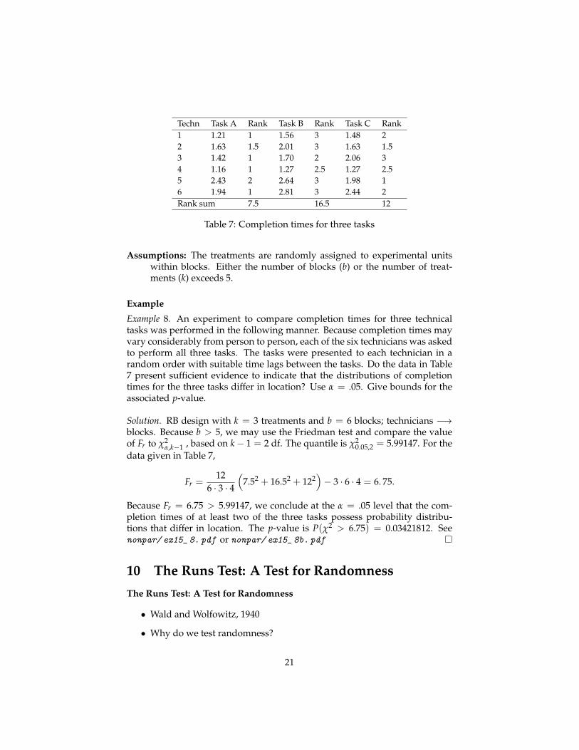
Techn Task A Rank Task B Rank Task C Rank1 1.21 1 1.56 3 1.48 22 1.63 1.5 2.01 3 1.63 1.53 1.42 1 1.70 2 2.06 34 1.16 1 1.27 2.5 1.27 2.55 2.43 2 2.64 3 1.98 16 1.94 1 2.81 3 2.44 2Rank sum 7.5 16.5 12

Table 7: Completion times for three tasks

Assumptions: The treatments are randomly assigned to experimental unitswithin blocks. Either the number of blocks (b) or the number of treat-ments (k) exceeds 5.

Example

Example 8. An experiment to compare completion times for three technicaltasks was performed in the following manner. Because completion times mayvary considerably from person to person, each of the six technicians was askedto perform all three tasks. The tasks were presented to each technician in arandom order with suitable time lags between the tasks. Do the data in Table7 present sufficient evidence to indicate that the distributions of completiontimes for the three tasks differ in location? Use α = .05. Give bounds for theassociated p-value.

Solution. RB design with k = 3 treatments and b = 6 blocks; technicians −→blocks. Because b > 5, we may use the Friedman test and compare the valueof Fr to χ2

α,k−1 , based on k− 1 = 2 df. The quantile is χ20.05,2 = 5.99147. For the

data given in Table 7,

Fr =12

6 · 3 · 4

(7.52 + 16.52 + 122

)− 3 · 6 · 4 = 6. 75.

Because Fr = 6.75 > 5.99147, we conclude at the α = .05 level that the com-pletion times of at least two of the three tasks possess probability distribu-tions that differ in location. The p-value is P(χ2 > 6.75) = 0.03421812. Seenonpar/ ex15_ 8. pdf or nonpar/ ex15_ 8b. pdf

10 The Runs Test: A Test for Randomness

The Runs Test: A Test for Randomness

• Wald and Wolfowitz, 1940

• Why do we test randomness?

21

• The runs test is used to study a sequence of events with one of two out-comes, success (S) or failure (F). If we think of the sequence of itemsemerging from a manufacturing process as defective (F) or nondefective(S), the observation of twenty items might yield

S S S S S F F S S SF F F S S S S S S S

• We notice the groupings of defectives and nondefectives and ask whetherthis grouping implies nonrandomness and, consequently, lack of processcontrol.

Definition 9. A run is a maximal subsequence of like elements.

• The 20 elements are arranged in five runs, the first containing five S’s, thesecond containing two F’s, and so on.

• A very small or very large number of runs in a sequence indicates non-randomness.

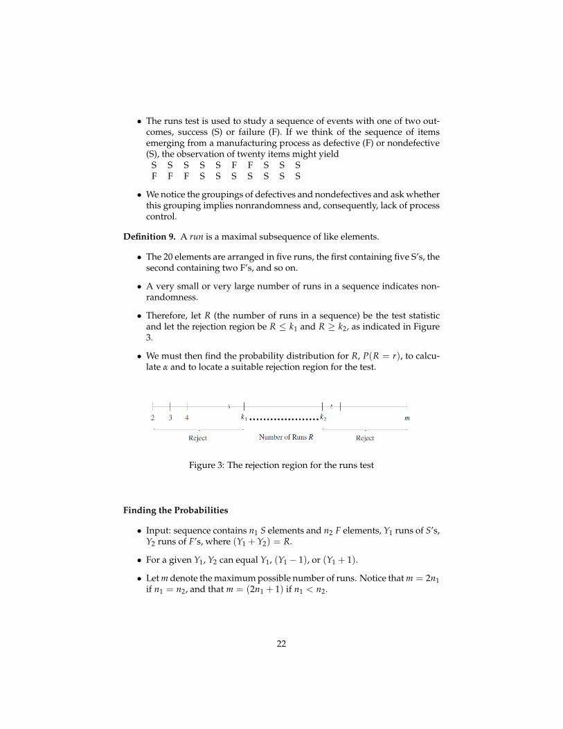
• Therefore, let R (the number of runs in a sequence) be the test statisticand let the rejection region be R ≤ k1 and R ≥ k2, as indicated in Figure3.

• We must then find the probability distribution for R, P(R = r), to calcu-late α and to locate a suitable rejection region for the test.

Figure 3: The rejection region for the runs test

Finding the Probabilities

• Input: sequence contains n1 S elements and n2 F elements, Y1 runs of S’s,Y2 runs of F’s, where (Y1 + Y2) = R.

• For a given Y1, Y2 can equal Y1, (Y1 − 1), or (Y1 + 1).

• Let m denote the maximum possible number of runs. Notice that m = 2n1if n1 = n2, and that m = (2n1 + 1) if n1 < n2.

22

• We will suppose that every distinguishable arrangement of the (n1 + n2)elements in the sequence constitutes a simple event for the experimentand that the sample points are equiprobable. It then remains for us tocount the number of sample points that imply R runs.

• The total number of distinguishable arrangements of n1 S elements andn2 F elements is (

n1 + n2n1

),

and therefore the probability per sample point is

1(n1 + n2

n1

) .

• The number of ways of achieving y1 S runs is equal to the number of iden-tifiable arrangements of n1 indistinguishable elements in y1 cells, none ofwhich is empty, as represented in Figure 4. This is equal to the numberof ways of distributing the (y1 − 1) inner bars in the (n1 − 1) spaces be-tween the S elements (the outer two bars remain fixed). Consequently, itis equal to the number of ways of selecting (y1 − 1) spaces (for the bars)out of the (n1 − 1) spaces available, or(

n1 − 1y1 − 1

).

• The number of ways of observing y1 S runs and y2 F runs, obtained byapplying the mn rule, is(

n1 − 1y1 − 1

)(n2 − 1y2 − 1

).

• This gives the number of sample points in the event “y1 runs of S’s andy2 runs of F’s.” The probability of exactly y1 runs of S’s and y2 runs ofF’s:

p (y1, y2) =

(n1 − 1y1 − 1

)(n2 − 1y2 − 1

)(

n1 + n2n1

)Then, P(R = r) equals the sum of p(y1, y2) over all values of y1 and y2such that (y1 + y2) = r.

• Examples: R = 4 could occur when y1 = 2 and y2 = 2 with either the Sor F elements commencing the sequences. Consequently,

P(R = 4) = 2P(Y1 = 2, Y2 = 2).

23

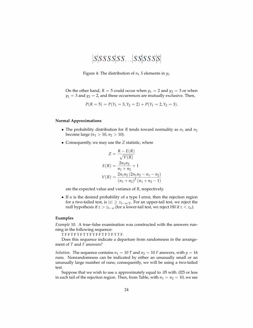
Figure 4: The distribution of n1 S elements in y1

On the other hand, R = 5 could occur when y1 = 2 and y2 = 3 or wheny1 = 3 and y2 = 2, and these occurrences are mutually exclusive. Then,

P(R = 5) = P(Y1 = 3, Y2 = 2) + P(Y1 = 2, Y2 = 3).

Normal Approximations

• The probability distribution for R tends toward normality as n1 and n2become large (n1 > 10, n2 > 10).

• Consequently, we may use the Z statistic, where

Z =R− E(R)√

V(R)

E(R) =2n1n2

n1 + n2+ 1

V(R) =2n1n2 (2n1n2 − n1 − n2)

(n1 + n2)2 (n1 + n2 − 1)

are the expected value and variance of R, respectively.

• If α is the desired probability of a type I error, then the rejection regionfor a two-tailed test, is |z| ≥ z1−α/2. For an upper-tail test, we reject thenull hypothesis if z > z1−α (for a lower-tail test, we reject H0 if z < zα).

Examples

Example 10. A true–false examination was constructed with the answers run-ning in the following sequence:

T F F T F T F T T F T F F T F T F T T F.Does this sequence indicate a departure from randomness in the arrange-

ment of T and F answers?

Solution. The sequence contains n1 = 10 T and n2 = 10 F answers, with y = 16runs. Nonrandomness can be indicated by either an unusually small or anunusually large number of runs; consequently, we will be using a two-tailedtest.

Suppose that we wish to use α approximately equal to .05 with .025 or lessin each tail of the rejection region. Then, from Table, with n1 = n2 = 10, we see

24

that P(R ≤ 6) = .019 and P(R ≤ 15) = .981. Then, P(R ≥ 16) = 1− P(R ≤15) = .019, and we would reject the hypothesis of randomness at the α = .038significance level if R ≤ 6 or R ≥ 16. Because R = 16 for the observed data,we conclude that evidence exists to indicate nonrandomness in the professor’sarrangement of answers. The attempt to mix the answers was overdone. Seenonpar/ ex15_ 10. pdf

Examples–cont.

• A second application – time series

• Departures from randomness in a series, caused either by trends or peri-odicities, can be detected by examining the deviations of the time seriesmeasurements from their average.

• Negative and positive deviations could be denoted by S and F, respec-tively, and we could then test this time sequence of deviations for non-randomness.

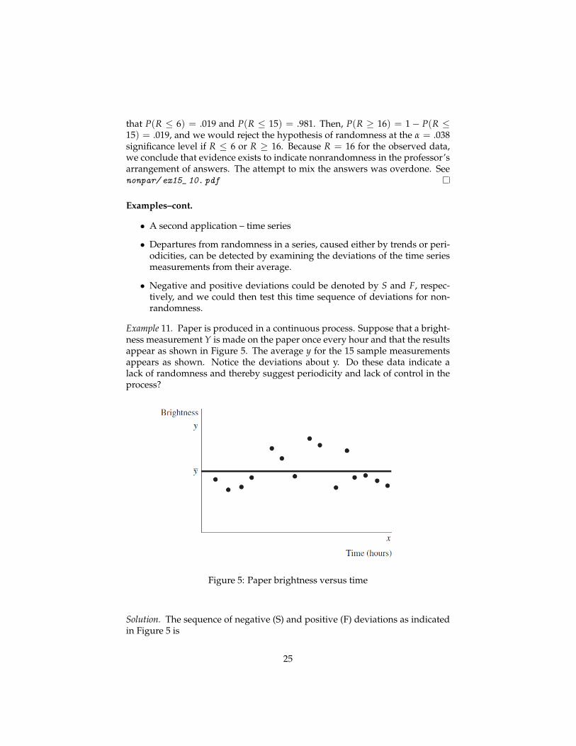
Example 11. Paper is produced in a continuous process. Suppose that a bright-ness measurement Y is made on the paper once every hour and that the resultsappear as shown in Figure 5. The average y for the 15 sample measurementsappears as shown. Notice the deviations about y. Do these data indicate alack of randomness and thereby suggest periodicity and lack of control in theprocess?

Figure 5: Paper brightness versus time

Solution. The sequence of negative (S) and positive (F) deviations as indicatedin Figure 5 is

25

S S S S F F S F F S F S S SThen, n1 = 10, n2 = 5, and R = 7. Consulting Table, we find P(R ≤ 7) =

.455. This value of R is not improbable, assuming the hypothesis of random-ness to be true. Consequently, there is not sufficient evidence to indicate non-randomness in the sequence of brightness measurements. See nonpar/ ex15_

11. pdf

11 Rank Correlation Coefficient

Rank Correlation Coefficient

• Let (X1, Y1), . . . , (Xn, Yn) be a random sample from a continuous bivari-ate population with joint distribution function FX,Y and marginal distri-bution functions FX and FY. That is, the (X, Y) pairs are mutually inde-pendent and identically distributed according to some continuous bivari-ate population.

• The null hypothesis: X and Y are independent:

H0 : [FX,Y(x, y) ≡ FX(x)FY(y), for all (x, y) pairs]. (4)

• To compute the Spearman rank correlation coefficient rs, we first orderthe n X observations from least to greatest and let Ri denote the rankof Xi, i = 1, . . . , n, in this ordering. Similarly, we separately order then Y observations from least to greatest and let Si denote the rank of Yi,i = 1, . . . , n, in this ordering. The Spearman (1904) rank correlation co-efficient is defined as the Pearson product moment sample correlation ofthe Ri and the Si.

• Recall that the sample correlation coefficient for observations (X1, Y1), . . . , (Xn, Yn)is given by

rP =Sxy√SxxSyy

=∑n

i=1(Xi − X)(Yi −Y)[∑n

i=1(Xi − X)2 ∑ni=1(Yi −Y)2

]1/2 .

• When no ties within a sample are present, this is equivalent to two com-putationally efficient formulae:

rS =

12n

∑i=1

(Ri − n+1

2

) (Si − n+1

2

)n (n2 − 1)

(5)

= 1−6 ∑n

i=1 D2i

n (n2 − 1), (6)

where Di = Ri − Si, i = 1, . . . , n.

26

• Rejection region

(a) Upper-tailed test: Ha : X and Y are positively associated. Reject H0 if rS ≥rS,α, where the constant rS,α is chosen to make the type I error probabilityequal to α. Values of rS,α are found with the command qSpearman.

(b) Lower-tailed test: Ha : X and Y are negatively associated. Reject H0 ifrS ≤ −rS,α

(c) Two-tailed test: Ha : X and Y are not associated (not independent). RejectH0 if |rS| ≥ rS,α/2.

The critical values are tabulated.

Normal Approximation

• The large-sample approximation is based on the asymptotic normality ofrS, suitably standardized. For this standardization, we need to know theexpected value and variance of rS when the null hypothesis of indepen-dence is true. Under H0, the expected value and variance of rS are

E(rS) = 0 (7)

V(rS) =1

n− 1. (8)

• The standardized version of rS is

r∗S =rS − E(rS)√

V(rS)=√

n− 1rS. (9)

• When H0 is true, r∗S has, as n tends to infinity, an asymptotic N(0, 1) dis-tribution.

Ties

• If there are ties among the n X observations and/or separately among then Y observations, assign each of the observations in a tied (either X or Y)group the average of the integer ranks that are associated with the tiedgroup.

• If there are tied X’s and/or tied Y’s, Spearman’s rank correlation coeffi-cient calculated with Pearson’s correlation does not require modification.

• If using the computationally efficient version of rS at (6), some changesto the statistic are necessary. The statistic rS in this case becomes

rS =n(n2 − 1)− 6 ∑n

s=1 D2s − 1

2 [T1 + T2]

{[n(n2 − 1)− T1] [n(n2 − 1)]− T2}1/2 (10)

27

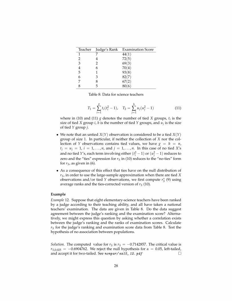
Teacher Judge’s Rank Examination Score1 7 44(1)2 4 72(5)3 2 69(3)4 6 70(4)5 1 93(8)6 3 82(7)7 8 67(2)8 5 80(6)

Table 8: Data for science teachers

T1 =g

∑i=1

ti(t2i − 1), T2 =

h

∑j=1

uj(u2j − 1) (11)

where in (10) and (11) g denotes the number of tied X groups, ti is thesize of tied X group i, h is the number of tied Y groups, and uj is the sizeof tied Y group j.

• We note that an untied X(Y) observation is considered to be a tied X(Y)group of size 1. In particular, if neither the collection of X nor the col-lection of Y observations contains tied values, we have g = h = n,tj = uj = 1, i = 1, . . . , n, and j = 1, . . . , n. In this case of no tied X’sand no tied Y’s, each term involving either (t2

i − 1) or (u2j − 1) reduces to

zero and the “ties” expression for rS in (10) reduces to the “no-ties” formfor rS, as given in (6).

• As a consequence of this effect that ties have on the null distribution ofrS, in order to use the large-sample approximation when there are tied Xobservations and/or tied Y observations, we first compute r∗S (9) usingaverage ranks and the ties-corrected version of rS (10).

ExampleExample 12. Suppose that eight elementary-science teachers have been rankedby a judge according to their teaching ability, and all have taken a nationalteachers’ examination. The data are given in Table 8. Do the data suggestagreement between the judge’s ranking and the examination score? Alterna-tively, we might express this question by asking whether a correlation existsbetween the judge’s ranking and the ranks of examination scores. CalculaterS for the judge’s ranking and examination score data from Table 8. Test thehypothesis of no association between populations.

Solution. The computed value for rS is rS = −0.7142857. The critical value isrS,0.025 = −0.6904762. We reject the null hypothesis for α = 0.05, left-tailed,and accept it for two-tailed. See nonpar/ ex15_ 12. pdf

28

References

References

[1] J. D. Gibbons, and S. Chakraborti. 2003. Nonparametric Statistical Inference,4th. ed. New York, Basel: Marcel Dekker

[2] Hollander, M., and D. A. Wolfe and E. Chicken. 2014. Nonparametric Sta-tistical Methods, 3rd ed. New York: Wiley.

[3] Kruskal, W. H., and W. A. Wallis. 1952. “Use of Ranks in One-CriterionVariance Analysis,” Journal of the American Statistical Association 47: 583–621.

29