optimization of gmr array sensor based magnetic flux
TRANSCRIPT

Optimization of GMR Array Sensor based
Magnetic Flux Leakage Techniques using
Finite Element Modeling
By
WAIKHOM SHARATCHANDRA SINGH
(Enrollment No: PHYS02200704005)
Indira Gandhi Centre for Atomic Research, Kalpakkam
A Thesis submitted to the
Board of Studies in Physical Sciences
In partial fulfillment of requirements
For the degree of
DOCTOR OF PHILOSOPHY
of
HOMI BHABHA NATIONAL INSTITUTE
July, 2013

Homi Bhabha National Institute
Recommendations of the Viva Voce Board
As members of the Viva Voce Board, we certify that we have read the dissertation
prepared by Waikhom Sharatchandra Singh entitled “Optimization of GMR Array
Sensor based Magnetic Flux Leakage Techniques using Finite Element Modeling”
and recommend that it may be accepted as fulfilling the dissertation requirement for the
Degree of Doctor of Philosophy.
_________________________________________________Date:
Chairman-Dr. R. S. Keshavamurthy
_________________________________________________Date:
Guide / Convener-Dr. B. Purna Chandra Rao
_________________________________________________Date:
Examinar: Dr. G. Rajaram
_________________________________________________Date:
Member 1-Dr. G. Amarendra
_________________________________________________Date:
Member 2- Dr. B. K. Panigrahi
Final approval and acceptance of this dissertation is contingent upon the
candidate‟s submission of the final copies of the dissertation to HBNI.

CERTIFICATE
I hereby certify that I have read this dissertation prepared under my direction
and recommend that it may be accepted as fulfilling the dissertation requirement.
I also certify that the thesis submitted to the examiners has been revised after
incorporating their suggestions. The revised thesis has been rebound and submitted to
the HBNI for the award of Degree of Doctor of Philosophy.
Guide - Dr. B. Purna Chandra Rao
Date:
Place: Kalpakkam

STATEMENT BY AUTHOR
This dissertation has been submitted in partial fulfillment of requirements for an
advanced degree at Homi Bhabha National Institute (HBNI) and is deposited in the
Library to be made available to borrowers under rules of the HBNI.
Brief quotations from this dissertation are allowable without special permission,
provided that accurate acknowledgement of source is made. Requests for permission for
extended quotation from or reproduction of this manuscript in whole or in part may be
granted by the Competent Authority of HBNI when in his or her judgment the proposed
use of the material is in the interests of scholarship. In all other instances, however,
permission must be obtained from the author.
(W. Sharatchandra Singh)
Date:
Place: Kalpakkam

DECLARATION
I, hereby declare that the investigation presented in the thesis entitled “Optimization of
GMR Array Sensor based Magnetic Flux Leakage Techniques using Finite Element
Modeling” submitted to Homi Bhabha National Institute (HBNI), Mumbai, India, for
the award of Doctor of Philosophy in Physical Sciences is the record of work carried
out by me under the guidance of Dr. B. Purna Chandra Rao, Head, Non-Destructive
Evaluation Division, Metallurgy and Materials Group, Indira Gandhi Centre for Atomic
Research, Kalpakkam. The work is original and has not been submitted earlier as a
whole or in part for a degree / diploma at this or any other Institution / University.
(W. Sharatchandra Singh)
Date:
Place: Kalpakkam

Solely dedicated to my Parents
Shri W. Shangaijaoba Singh
And (Late) Smt. W. Mema Devi

ACKNOWLEDGEMENT
I owe my deep sense of gratitude to my research supervisor and mentor Dr. B. Purna
Chandra Rao, Head, Non-Destructive Evaluation Division (NDED), Indira Gandhi
Centre for Atomic Research (IGCAR) for his whole hearted support, encouragement
and guidance during the research work. Without his untiring mentorship, constant
inspiration, valuable discussions and suggestions, this thesis wouldn‟t have been
possible. I am deeply obliged to his meticulous planning, effective approach and
perfections in all the research works.
I express my sincere gratitude to Dr. T. Jayakumar, Director, Metallurgy and
Materials Group, IGCAR for his inspiration, encouragement and most importantly
providing direction during the course of thesis work. I would like to extend my heartfelt
thanks to Dr. Baldev Raj and Shri S. C. Chetal, the former Directors, IGCAR and Dr.
P. R. Vasudeva Rao, the present Director, IGCAR for permitting me to pursue research
in this reputed centre.
My sincere thanks to my Doctoral Committee members Dr. R. S. Keshavamurthy, Dr.
B. Purna Chandra Rao, Dr. G. Amarendra and Dr. B. K. Panigrahi for regular
evaluation of the research work and giving many useful suggestions.
I take this opportunity to thank Dr. C. K. Mukhopadhyay, Shri S. Mahadevan, Shri
S. Thirunavukkarasu, Smt. B. Sasi and Shri A. Viswanath, NDE Division who
helped me to learn various technical ingredients for analysis of the results. I am grateful
to Shri P. Krishnaiah for helping me to wind the coils and to make the magnetisation
units. Thanks to all the staffs of NDE Division for all the helpful assistance.

My special thanks to my friend Dr. Satender Kataria and his family members for
encouragement and precious help to my family, in many times. I also thank to my
friends Dr. S. Ayyapan, Dr. C. Pandian and Dr. Satyaprakash Sahoo for valuable
discussions and suggestions during their stay at Kalpakkam. I also would like to
acknowledge Dr. K. Sathpathy, Shri Shuaib Ahmed, Dr. N. Joyshankar, Shri C.
Kisan and Shri L. Herojit for their kind helps in many situations.
My appreciation is also offered to my wife Smt. W. Langlentombi Devi and daughters
Kum. W. Santirani, Kum. W. Babyrani and Kum. W. Kriparani for their
understanding, support and patience during my research work.
(W. Sharatchandra Singh)

CONTENTS
Page No.
Synopsis…………………………………………………………………….. i
List of Figures……………………………………………………………… iii
List of Tables……………………………………………………..………... xi
List of Abbreviations………………………………………..…………….. xii
List of Publications and Awards……………………………………..…… xv
Chapter 1 Introduction……………………………………………... 1
1.1 Introduction to Nondestructive Testing (NDT)………….. 1
1.2 Introduction to Magnetic Flux Leakage (MFL)
Testing………………………………………………………
5
1.2.1 Working Principle…………………………………... 5
1.2.2 Capabilities…………………………………………. 7
1.2.3 Applications…………………………………............ 7
1.3 Magnetisation Techniques in MFL Testing……………... 9
1.3.1 Permanent Magnets………………………………… 9
1.3.2 Electromagnets……………………………………... 10
1.3.2.1 Electromagnetic Yoke……………………… 10
1.3.2.2 Solenoid Coil……………………………….. 11
1.3.2.3 Helmholtz Coils…………………………….. 12
1.3.3 Electric Current……………..……………………… 13
1.4 Magnetic Field Sensors for MFL Testing………………... 14
1.4.1 Induction Coils…………………………………………... 14

1.4.2 Hall Sensors……………………………………………… 15
1.4.3 SQUID Sensors………………………………………….. 16
1.4.4 AMR Sensors…………………………………………….. 16
1.4.5 GMR Sensors…………………………………………….. 17
Chapter 2 Literature Review and Motivation……………... 21
2.1 Literature Review…………………………………………. 21
2.1.1 Modeling of MFL Testing.………………………….. 22
2.1.1.1 Theoretical Modeling……………………….. 23
2.1.1.2 Numerical Modeling………………………... 28
2.2 Motivation………………………………………………….. 34
2.3 Objective of the Thesis……………………………………. 35
2.4 Organization of the Thesis………………………………... 36
Chapter 3 Finite Element Modeling of MFL Technique…... 38
3.1 Introduction to Finite Element Modeling………………... 38
3.1.1 Discretization of Domain………………………………. 39
3.1.2 Selection of Interpolation Functions………………….. 40
3.1.3 Formulation of System of Equations…………………. 41
3.1.4 Solution of System of Equations……………………. 41
3.1.5 Post-processing of Data………………………………... 42
3.2 Finite Element Modeling of MFL Technique…………… 43
3.2.1 Construction of Model Geometry…………………... 43
3.2.2 Mathematical Formulation…………………………….. 44
3.2.2.1 Governing Equation………………………... 44
3.2.2.2 Boundary Conditions………………………. 48
3.2.3 Meshing…………………………………………….. 49
3.2.4 Solver……………………………………………….. 50
3.2.5 Post-processing and Prediction of GMR
Signal….....................................................................
51
3.3 Validation of Model……………………………………... 52
Chapter 4 Optimization of MFL Technique for Cuboid
Geometry………………………………………….
55
4.1 Introduction………………………………………………... 55
4.2 MFL Technique for Cuboid Geometry…………………. 57
4.3 Modeling………………………………………………….... 57
4.4 Experimental Setup……………………………………….. 67
4.5 Reference Defects……………………………………….... 68
4.6 Experimental Results……………………………………… 71
4.6.1 Surface Defects……………………………………... 71
4.6.2 Sub-surface Defects………………………………… 73
4.6.3 Influence of Lift-off on MFL Signals………………... 76
4.6.4 Influence of Inclined Defects on MFL Signals……... 76
4.6.5 Influence of Interacting Defects on MFL Signals….. 79
4.6.6 Validation…………………………………………… 80
4.7 Development of 2-dimensional 16 Element GMR Array
Sensors……………………………………………………...
82
4.8 Conclusions………………………………………………… 84
Chapter 5 Optimization of MFL Technique for Solid
Cylindrical Geometry……………………………
86
5.1 Introduction………………………………………………... 86

5.2 MFL Technique for Solid Cylindrical Geometry……….. 89
5.3 Modeling…………………………………………………… 90
5.4 Experimental Setup……………………………………….. 94
5.5 Reference Defects………………………………………… 95
5.6 Experimental Results……………………………………… 96
5.6.1 Local Flaws………………………………………… 96
5.6.2 Loss of Metallic Cross-sectional Area……………… 101
5.6.3 Validation…………………………………………… 102
5.6.4 Comparative Performance of Saddle Coils and
Helmholtz Coil Magnetisations……………………..
104
5.7 Development of Flexible 12 Element GMR Array
Sensors……………………………………………………...
106
5.8 Conclusions………………………………………………… 110
Chapter 6 Optimization of MFL Technique for Hollow
Cylindrical Geometry……………………………
112
6.1 Introduction……………………………………………….. 112
6.2 MFL Technique for Hollow Cylindrical Geometry……... 116
6.3 Modeling…………………………………………………… 117
6.4 Experimental Setup……………………………………….. 125
6.5 Reference Defects………………………………………… 126
6.6 Experimental Results……………………………………… 127
6.6.1 Localised Defects…………………………………… 127
6.6.2 Influence of Support Plate on MFL Signals………... 131
6.6.3 Validation…………………………………………… 133

6.7 Development of Flexible 5 Element GMR Array Sensors. 134
6.8 Conclusions………………………………………………… 136
Chapter 7 Generalized Approach Proposed for Model
based Optimization……….……………..…….…
138
7.1 Comparative Performance of MFL Techniques for the
Three Different Geometries……………………………….
138
7.2 Generalized Approach……………………………………. 140
Chapter 8 Conclusions………………………………………. 142
Chapter 9 Future Work……………………………………... 145
References………………………………………………... 147

i
SYNOPSIS
This thesis presents the three dimensional finite element (3D-FE) model based
optimization of magnetic flux leakage (MFL) techniques for high sensitive, fast and
reliable non-destructive detection of defects in ferromagnetic components of three
different geometries viz. 1) cuboid geometry, 2) solid cylindrical geometry and 3)
hollow cylindrical geometry. Carbon steel plates, track ropes of Heavy Water Plant
(HWP) and steam generator (SG) tubes of Prototype Fast Breeder Reactor (PFBR) have
been considered for cuboid, solid cylindrical and hollow cylindrical geometries,
respectively. Experiments have been conducted to confirm the effectiveness of the
model based optimization of MFL techniques using giant magneto-resistive (GMR)
sensors connected to low-noise differential amplifiers and to develop array sensors for
rapid imaging of defects.
Optimization of MFL technique for carbon steel plates (thickness, 12 mm) has
been carried out by optimizing the leg spacing, height and magnetizing current of the
electromagnetic yoke used in the technique. Confirming experiments have been
conducted. GMR sensor with a low-noise differential amplifier have enabled successful
detection of a sub-surface notch (depth, 0.9 mm) located at 11.1 mm below the surface.
The MFL signal parameters namely, skewness and Bx-Bz locus patterns have been found
to be useful for enhanced detection and classification of inclined and interacting defects
in cuboid geometry.
MFL technique that uses saddle coils and GMR array sensors has been
developed, for the first time, for inspection of track ropes (outer diameter, 64 mm)
representing solid cylindrical geometry. The magnetizing current, inter-coil spacing of

ii
the saddle coils and locations of GMR sensors between the two coils have been
optimized using the 3D-FE model. The experimental results clearly confirmed the
reliable detection of both localized flaw (LF) and loss of metallic area (LMA) type
defects and resolution (3.2 mm) of multiple flaws in the track rope. Further, a novel
flexible 12 element GMR array sensor has been developed and successfully used for
rapid imaging to obtain the spatial information of both LF and LMA type defects.
For optimization of MFL technique for testing SG tubes (outer diameter, 17.2
mm and wall thickness, 2.3 mm) using GMR array sensors, the magnetisation unit
comprising of two bobbin coils wound on a ferrite core has been optimized for
achieving optimum inter-coil spacing of the bobbin coils. The number of GMR sensors
and their locations have been optimized by predicting the uniform magnetic flux density
region between the two bobbin coils. A 5-element GMR array sensor has been
fabricated and the performance of the GMR array sensor has been evaluated for
successful detection and imaging of 1 mm diameter localized hole in the tube. The
influence of support plate and sodium deposits on the tube outer surface and in defect
regions on the MFL signals has been analysed, for the first time.
This thesis finally proposes a generalized approach for optimization of MFL
techniques using finite element modeling for enhanced detection and fast imaging of
defects in ferromagnetic components, without the need for extensive physical testing.

iii
LIST OF FIGURES
Fig. No. Fig. Caption Page No.
Fig. 1.1 A generic NDE system……………………………………….. 2
Fig. 1.2 (a) Typical magnetisation curve and (b) ferromagnetic test
object with defect illustrating MFL method……………….….
6
Fig. 1.3 Online MFL inspection of pipelines using
PIGs…………………………………………………………...
8
Fig. 1.4 GMR multilayer structures…………………………………… 18
Fig. 1.5 GMR effect…………………………………………………… 19
Fig. 2.1 (a) Two-dimensional rectangular defect below the specimen
surface and (b) its modified double dipole model…………….
26
Fig. 2.2 Computed leakage magnetic field signals for (a) tangential
and (b) normal components of surface and sub-surface slots
in ferromagnetic material……………………………………..
26
Fig. 2.3 MFL signal peak-to-peak amplitudes as functions of (a)
defect width (length 10 mm, depth 10 mm) in a 14 mm thick
plate and (b) defect depth (length 10 mm, width 10 mm) in a
10 mm thick plate at various lift-offs…………………………
31
Fig. 3.1 (a) One-dimensional, (b) two-dimensional and (c) three-
dimensional basic finite elements…………………………….
40
Fig. 3.2 3D-FE model geometry for MFL NDE of steel plate………... 44
Fig. 3.3 Typical meshing for 3D-FE modeling of MFL technique of 50

iv
steel plate……………………………………………………...
Fig. 3.4 FE model predicted arrow contour plots for (a) surface slot of
3.32 mm depth and (b) sub-surface slot located at 6.24 mm
below the measurement surface………………………………
51
Fig. 3.5 Magnetization curve for steam generator tube ….…………. 54
Fig. 3.6 Comparison of model predicted and experimentally obtained
(a) MFL signals for circumferential notches and (b) its signal
peak amplitudes……………………………………………….
54
Fig. 4.1 Three different structures of C-core electromagnetic yoke for
MFL NDE of cuboid geometry……………………………….
58
Fig. 4.2 Model predicted contour lines of Bx component of magnetic
flux density from the surface groove for (a) structure 1 (b)
structure 2 and (c) structure 3………………………………....
62
Fig. 4.3 Model predicted Bx component of MFL signals for (a) surface
groove and (b) sub-surface groove of the three yoke
structures……………………………………………………...
62
Fig. 4.4 Model predicted Bxpeak
amplitudes for surface and sub-surface
grooves of the three yoke structures…………………………..
63
Fig. 4.5 Model predicted variation of Bxpeak
amplitudes with (a)
height, (b) leg spacing of yoke, (c) lift-off and (d) plate
thickness for the surface and sub-surface groove……………
64
Fig. 4.6 Model predicted Bxpeak
amplitudes of MFL signals as a
function of magnetising current ………………………..…..
66

v
Fig. 4.7 Schematic of experimental setup used for MFL
measurements on carbon steel plate…………………………..
67
Fig. 4.8 (a) Functional block diagram of GMR bridge sensor and (b)
GMR sensor response characteristic………………………….
68
Fig. 4.9 Carbon steel plate specimen with EDM notches…………….. 69
Fig. 4.10 Schematic showing (a) surface notch (near-side) and (b) sub-
surface notch (far-side)……………………………………….
71
Fig. 4.11 GMR sensor signal output for various surface notches of (a)
0.5 mm width and (b) 1.0 mm width………………………....
72
Fig. 4.12 GMR signal amplitude as a function of depth for surface
notches (dotted line shows the approximated two-slope
behavior)……………………………………………………...
73
Fig. 4.13 GMR sensor signal response for sub-surface notches of (a)
0.5 mm width and (b) 1.0 mm width located at different
depths below surface………………………………………….
75
Fig. 4.14 GMR sensor signal amplitude for sub-surface notches as a
function of notch location below the surface………………....
75
Fig. 4.15 Variation of GMR signal amplitude with lift-off for different
sub-surface notches …………………………………………
76
Fig. 4.16 (a) Measured GMR sensor signal response for inclined
notches, (b) parameters determined from the measured MFL
signals, (c) signal asymmetry and (d) differential skewness as
a function of angle of inclination of notches………………….
79

vi
Fig. 4.17 (a) Measured GMR sensor signal response for interacting
notches and (b) ratio of peak amplitudes of outer and inner
flanks as a function of notch-to-notch separations……………
80
Fig. 4.18 Comparison between the model and experimentally obtained
(a) MFL signal amplitude as a function of notch location
below the surface for sub-surface notches and (b) differential
skewness as a function of angle of inclination for inclined
notches………………………………………………………...
81
Fig. 4.19 (a) Model predicted magnetic flux density between the legs
of the electromagnetic yoke (b) the photograph of fabricated
2D array of 4x4 GMR sensors………………………………..
83
Fig. 4.20 (a) 16 element 2D GMR array sensor response for a 3.32 mm
deep surface notch and (b) its corresponding MFL image......
84
Fig. 5.1 The cross-section and design details of double locked track
rope……………………………………………………………
88
Fig. 5.2 (a) Photograph of the track rope system with bucket carrying
coal and (b) local flaws and loss of metallic cross-sectional
area on the outer surface of the track rope…………………...
89
Fig. 5.3 Breakage of wires at the outer surface of the track rope……... 89
Fig. 5.4 Three different structures of coil based magnetising unit for
MFL NDE of track ropes……………………………………..
90
Fig. 5.5 (a) 3D finite element mesh and model predicted magnetic
flux line contours between the two saddle coils for (b)
92

vii
clockwise and (c) anticlockwise directions of electric currents
Fig. 5.6 Optimization of (a) magnetising current and (b) inter-coil
spacing between the two saddle coils………………………...
94
Fig. 5.7 Experimental setup for the MFL testing of track ropes……… 95
Fig. 5.8 Schematic of the track rope having axial and circumferential
machined artificial notches…………………………………...
96
Fig. 5.9 MFL signals for (a) axial notches and (b) circumferential
notches………………………………………………………..
97
Fig. 5.10 FWHM and signal amplitude for axial and circumferential
notches………………………………………………………..
98
Fig. 5.11 (a) Photograph of the saw cut in the track rope and (b) the
corresponding GMR sensor output…………………………...
99
Fig. 5.12 (a) Photograph of 5 saw cuts (23.2 mm length, 1.0 mm width
and 2.0 mm depth) separated by 13.5 mm, 10.0 mm, 5.5 and
3.2 mm distances and (b) the corresponding GMR sensor
measured MFL signals………………………………………..
100
Fig. 5.13 Photograph of LMA (42.0 mm length, 9.2 mm width and 3.0
mm depth) machined in the track rope and its GMR sensor
response scanned along dotted line AA direction…………….
101
Fig. 5.14 (a) Model predicted MFL signals from the axial notch, C and
the circumferential notch, G and (b) the corresponding
experimentally measured GMR sensor response…………….
102
Fig. 5.15 Comparison of model predicted and experimentally measured 103

viii
(a) normalised MFL signal amplitude of circumferential LFs
and (b) MFL signal of LMA………………………………….
Fig. 5.16 Schematic of Helmholtz coil magnetisation based MFL
testing set-up………………………………………………….
105
Fig. 5.17 MFL signals for (a) axial notches and (b) circumferential
notches using Helmholtz coil magnetisation…...…………….
106
Fig. 5.18 (a) Model predicted magnetic flux density between the saddle
coils along half of circumferential distance and (b) the
fabricated flexible sensor array of 12 GMR sensors…………
107
Fig. 5.19 Photographs of (a) axial LF, (b) circumferential LF, (c) axial
LMA and (d) circumferential LMA type defects in the track
rope……………………………………………………………
108
Fig. 5.20 GMR sensor array response for a 5.5 mm long
circumferential LF…………………………………………….
108
Fig. 5.21 MFL images for (a) axial and (b) circumferential LFs………. 109
Fig. 5.22 MFL images of (a) axial LMA (42.0 x 9.0 x 3.0 mm3) and (b)
circumferential LMA (33.5 x 14.2 x 4.9 mm3)……………….
110
Fig. 6.1 (a) Schematic of steam generator and (b) photograph of tube
bundle assembly………………………………………………
113
Fig. 6.2 MFL technique proposed for small diameter SG tubes of
hollow cylindrical geometry………………………………….
117
Fig. 6.3 Three different core structures of bobbin coils based
magnetising unit for MFL NDE of small diameter hollow
119

ix
cylinder……………………………………………………….
Fig. 6.4 Surface and arrow plots of magnetic flux density from a 1.15
mm deep OD notch for (a) air core, (b) ferrite core and (c)
ferrite core with flux guide (d) air core (near defect), (e)
ferrite core (near defect) and (f) ferrite core with flux guide
(near defect)………………………………..………………...
121
Fig. 6.5 Model predicted Ba component of MFL signals for (a) ID
notch and (b) OD notch of three magnetising coil structures...
122
Fig. 6.6 Model predicted Bapeak
amplitudes of MFL signals for ID and
OD notches of three magnetising coil structures……………..
123
Fig. 6.7 Optimization of (a) inter-coil spacing between the two bobbin
coils and (b) magnetising current…………………………….
124
Fig. 6.8 (a) Experimental setup for MFL testing of SG tube and (b)
photograph of GMR sensor based MFL probe………………
126
Fig. 6.9 GMR sensor response for outer side (a) EDM circumferential
notches, (b) flat bottom holes and (c) through holes in SG
tube……………………………………………………………
129
Fig. 6.10 GMR sensor signal amplitude as a function of volume of
defects………………………………………………………...
130
Fig. 6.11 (a) Photograph of the SG tube with support plate (Inconel-
718) and (b) comparison of experimentally obtained and
model predicted MFL signals for a 1.08 mm diameter hole in
tube with and without the support plate……………………..
132

x
Fig. 6.12 Model predicted contour plots of magnetic flux density (a)
with and (b) without the support plate………………………..
133
Fig. 6.13 Comparison of experimentally obtained and model predicted
MFL signal amplitude of circumferential notches.
134
Fig. 6.14 (a) Model predicted magnetic flux density between the two
bobbin coils (b) the photograph of fabricated flexible array of
5 element GMR sensors………………………………………
135
Fig. 6.15 Response of 5 element GMR array sensor for through holes
of 1.1, 2.0, 2.8 and 3.1 mm diameter………………………....
135
Fig. 7.1 Flowchart of the generalized approach for model based
optimization of MFL techniques………………………...…....
141

xi
List of Tables
Table No. Table Caption Page No.
Table 1.1 Comparison of commonly used sensors in MFL testing…. 19
Table 3.1 Parameters used in the FE modeling………………………. 53
Table 4.1 Parameters used in the FE modeling of MFL technique for
carbon steel plate…………………………………………...
59
Table 4.2 Details of surface and sub-surface notches in 12 mm thick
carbon steel plates………………………………………….
70
Table 5.1 Details of artificial EDM notches machined in the track
rope (length 5.5 mm and width 2.0 mm)…………………...
96
Table 6.1 Parameters used in the FE modeling of MFL technique….. 119
Table 6.2 Depths of reference defects in SG tubes…………………... 127
Table 7.1 Comparative performance of MFL techniques for the three
different geometries………………………………………..
139

xii
List of Abbreviations
Symbol Abbreviation
1D, 2D, 3D One-dimension, two-dimension, three-dimension
Ф Magnetic flux
σ Surface magnetic charge density
ρ Volume magnetic charge density
μ0 Magnetic permeability of free space
μr Relative permeability
a0, a1 Coefficients
A Magnetic vector potential
Ax, Ay and Az Components of vector potential
AC Alternating current
AMR Anisotropic magneto-resistive
AST Above ground storage tank
{b} Global source vector
, , Vectors of an element e
Bx, By, Bz Tangential, circumferential and normal components of
leakage flux density
Bxpeak
, Bzpeak
MFL peak amplitudes
Bxlpeak
- Bxrpeak
Difference in peak amplitudes w. r. t. left and right minima
BEM Boundary element method
CG Conjugate gradient
DC Direct current
ECT Eddy current testing
EDM Electro-discharge machining
F(A) Functional
FDM Finite difference method
FE Finite element
FEM Finite element method
FGMRES Flexible generalised minimum residual

xiii
FWHM Full width at half maximum
GMR Giant magneto-resistive
GMRES Generalised minimum residual
h Defect location below the specimen surface
hy Height of yoke
H0 Applied magnetic field
Hx, Hz Tangential and normal components of leakage field intensity
Hs*
Effective magnetic field in the specimen
HWAC Half wave rectified current
HWP Heavy water plant
I Magnetising current
ID Internal diameter
ILI In-line inspection
IRIS Internal rotary ultrasonic inspection
ISI In-service inspection
J Current density
[K] Global matrix (or stiffness matrix)
, , Matrices of an element e
LF Local flaws
LMA Loss of metallic cross-sectional area
LPT Liquid Penetrant testing
M Magnetisation
MFL Magnetic flux leakage
MPT Magnetic particle testing
MR Magneto-resistive
N Number of copper winding turns
Nje Interpolation function of element e at node j
NDE Non-destructive evaluation
NDT Non-destructive testing
NVE Non volatile electronics

xiv
OD Outer diameter
PCB Printed circuit board
PFBR Prototype fast breeder reactor
PIG Pipe inspection gauge
PSEC Partial saturation eddy current
RH Hall coeffcient
RFEC Remote field eddy current
RMS Root mean square error
RT Radiographic testing
sc Inter-coil spacing of bobbin coils
ss Inter-coil spacing of saddle coils
sy Leg spacing of yoke
SG Steam generator
SQUID Superconducting quantum interface device
SNR Signal-to-noise ratio
UT Ultrasonic testing
VH Hall voltage
VT Visual testing
WT Wall thickness

xv
List of Publications
Publications in Journals
1. W. Sharatchandra Singh, B. P. C. Rao, S. Thirunavukkarasu, C. K. Mukhopadhyay
and T. Jayakumar, “Design and optimization of GMR array based magnetic flux
leakage probe for imaging of defects in small diameter steam generator tubes”, Sensors
and Actuators A (Communicated).
2. W. Sharatchandra Singh, B. P. C. Rao, S. Thirunavukkarasu, C. K. Mukhopadhyay
and T. Jayakumar, “GMR based magnetic flux leakage technique for detection of
localized outer side defects in small diameter ferromagnetic steam generator tubes”,
IEEE Transactions on Magnetics (Communicated).
3. W. Sharatchandra Singh, B. P. C. Rao, S. Thirunavukkarasu and T. Jayakumar,
“Flexible GMR sensor array for magnetic flux leakage testing of steel track ropes”,
Journal of Sensors, vol. 2012, article ID 129074, 6 pages, March 2012.
4. W. Sharatchandra Singh, B. P. C. Rao, S. Thirunavukkarasu, S. Mahadevan, C. K.
Mukhopadhyay and T. Jayakumar, “3-D finite element modeling of leakage magnetic
fields from inclined cracks in carbon steel plates”, Studies in Applied Electromagnetics
and Mechanics, Electromagnetic Nondestructive Evaluation (XV), vol. 36, pp. 175-182,
January 2012.
5. W. Sharatchandra Singh, B. P. C. Rao, C. K. Mukhopadhyay and T. Jayakumar,
“GMR based magnetic flux leakage technique for condition monitoring of steel track
rope”, Insight, vol. 53, no. 7, pp. 377-381, July 2011.

xvi
6. W. Sharatchandra Singh, B. P. C. Rao, S. Mahadevan, T. Jayakumar and Baldev
Raj, “Giant magneto-resistive sensor based magnetic flux leakage technique for
inspection of track ropes”, Studies in Applied Electromagnetics and Mechanics,
Electromagnetic Nondestructive Evaluation (XIV), vol. 35, pp. 256-263, June 2011.
7. W. Sharatchandra Singh, B. P. C. Rao, T. Jayakumar and Baldev Raj,
“Simultaneous measurement of tangential and normal components of leakage magnetic
flux using giant magneto-resistive sensors”, Journal of Non-Destructive Testing &
Evaluation, vol. 8, no. 2, pp. 23-28, September 2009.
8. W. Sharatchandra Singh, B. P. C. Rao, S. Vaidyanathan, T. Jayakumar and Baldev
Raj, “Detection of leakage magnetic flux from near-side and far-side defects in carbon
steel plates using giant magneto-resistive sensor”, Measurement Science and
Technology, vol. 19, no. 1, 015702 (8pp), January 2008.
Conference Proceedings
1. W. Sharatchandra Singh, B. P. C. Rao, C. K. Mukhopadhyay and T. Jayakumar,
“Giant magneto-resistive sensor array for non-destructive detection of leakage magnetic
flux from surface defects in ferromagnetic materials”, International Conference On
Sensors and Related Networks (SENNET 12), VIT University, India, pp. 71-73, January
2012.
2. W. Sharatchandra Singh, S. Thirunavukkarasu, S. Mahadevan, B. P. C. Rao, C. K.
Mukhopadhyay and T. Jayakumar, “Three-dimensional finite element modeling of
magnetic flux leakage technique for detection of defects in carbon steel plates”, Proc. of
COMSOL Conference-2010, Bangalore, India, October 2010 (CD released).

xvii
3. W. Sharatchandra Singh, K. Krishna Nand, B. P. C. Rao, T. Jayakumar and Baldev
Raj, “Magnetic flux leakage NDE using giant magneto-resistive sensors”, Review of
Progress in Quantitative NDE, AIP Press, vol. 27B, pp. 857-864, March 2008.
4. W. Sharatchandra Singh, B. P. C. Rao, B. Sasi, S. Vaidyanathan, T. Jayakumar and
Baldev Raj, “Giant magneto-resistive sensors for non-destructive detection of magnetic
flux leakage from sub-surface defects in steels”, International Conference On Sensors
and Related Networks (SENNET 07), VIT University, India, pp. 11-14, December
2007.
Awards
1. Best oral presentation award for presenting a paper entitled “Three-dimensional
finite element modeling of magnetic leakage flux from inclined and interacting defects”,
W. Sharatchandra Singh, S. Thirunavukkarasu, S. Mahadevan, B. P. C. Rao, C. K.
Mukhopadhyay and T. Jayakumar, NDE Seminar-2010, Kolkata, India, December
2010.
2. Best oral presentation award for presenting a paper entitled “Three-dimensional
finite element modeling of magnetic flux leakage technique for detection of defects in
carbon steel plates”, W. Sharatchandra Singh, S. Thirunavukkarasu, S. Mahadevan, B.
P. C. Rao, C. K. Mukhopadhyay and T. Jayakumar, COMSOL Conference-2010,
Bangalore, India, October 2010.

Chapter 1
1
Chapter 1: Introduction
1.1 Introduction to Non-Destructive Testing
Assessment of structural integrity of engineering components and structures in many
industries is essential for ensuring their safe and economical operations. In general,
components and structures fail due to the presence and growth of inherent or service-
induced defects. Sometimes failures can occur without any prior notice. This has
motivated the search for techniques for detection and quantitative characterization of
defects to take corrective actions to prevent failures of catastrophic consequences. Very
often, assessment of structural integrity of a component is performed through
mechanical destructive tests which measure properties such as hardness, tensile strength
and ductility. However, inspection of installed components such as steam generator
(SG) in nuclear plants, pipelines in petrochemical industries, etc. demands techniques
that are non-destructive.
Non-destructive testing (NDT) is a branch of material science that deals with the
assessment of soundness and structural integrity of a component or structure through
detection of defects without causing any damage to it [1-2]. This mere detection of
defects is not sufficient to take the decision of acceptance/rejection of the component.
This has lead to the emergence of non-destructive evaluation (NDE) as a new discipline
which does detection as well as quantification of defects with respect to its shape, size,
location, and orientation. NDE also involves characterization of microstructures,
residual stresses and degradation of mechanical properties of components or structures.

Chapter 1
2
NDE is being routinely used in nuclear power plants, transportation, aerospace
and petrochemical industries to ensure reliability, safety and structural integrity of
critical components such as heat exchangers, railroads, aircraft engines, wire ropes, gas
pipelines and others where failures can effect availability factors, productivity and
profitability[3-4]. The NDE of installed critical components is becoming increasingly
important for both safety and economic reasons. There is a tremendous demand for new
and improved NDE techniques that are efficient, reliable and economical to use in many
industries.
Figure 1.1 shows a generic NDE system consisting of a specimen under test, an
excitation source and a receiving sensor array. The excitation source interacts with the
test specimen. If any defect is present in the specimen, the interaction of the field is
different for defective and healthy regions of the specimen. This difference in
interaction response is measured using the sensor array. The sensor array output in the
form of signals or images is further analyzed using signal or image processing
techniques to display the useful information of the defect.
Figure 1.1 A generic NDE system.

Chapter 1
3
There are several established NDE methods which are based on various physical
principles. Commonly used NDE methods include the following:
Visual Testing (VT)
Liquid Penetrant Testing (LPT)
Ultrasonic Testing (UT)
Radiographic Testing (RT)
Eddy Current Testing (ECT)
Magnetic Particle Testing (MPT)
Among these methods, visual testing is the oldest and the least expensive method
which is generally used as the first step for assessing the overall general health of a
component and for detection of surface-breaking defects. A variety of aids such as
magnifying glass, fibrescopes, cameras and video equipments are often used to enhance
the capability of VT method. The basic principle of liquid penetrant testing is to
increase the visibility contrast between defect and background by applying a liquid of
high mobility and penetrating power to the region of interest, and then allowing the
liquid to emerge from the developer to reveal the defect pattern under white light or
ultraviolet light. The LPT method is applicable to all types of materials and component
geometries. Ultrasonic testing uses high frequency (0.5 - 25 MHz) sound waves to
detect imperfections or changes in material properties within a specimen. It is a
volumetric technique and can detect cracks, laminations, shrinkage, cavities, pores and
inclusions in plates, pipes, welds, castings and forgings [5]. Radiographic testing uses
an x-ray tube or radioactive isotope as a source of radiation which passes through the

Chapter 1
4
material and captures the radiation on a film or digital device placed on the opposite
side. Possible imperfections are identified in radiographic images through density
changes. RT is widely used for volumetric inspection of castings, welds, bonded
structures and composite materials. Eddy current testing method works on the principle
of electromagnetic induction and measures changes in coil impedance due to variations
in electrical conductivity and magnetic permeability in metallic materials. ECT method
is widely used for materials sorting, defect detection in tubes, sheets and rods and
coating thickness measurements [6-8]. It is also possible to assess heat treatment
adequacy and microstructure degradation [6]. In magnetic particle testing (MPT)
method, the test component is magnetised and local magnetic flux leakage due to
presence of defects is detected using fine magnetic particles [9]. MPT is widely used for
inspection of cracks in crankshafts, fly wheels, crank hooks in transportation industries,
butt welds of pressure vessels and steam turbine rotors in power plants, etc. [5, 9].
However, it fails to test parts such as inner diameter defects of long tubes and pipes etc.,
which are not easily accessible for visual examination [10]. Often demagnetisation and
cleaning of the object is required after carrying out the MPT. It does not provide
permanent and quantitative records of inspection and its capability is limited for
detection of sub-surface defects located beyond 5 mm from surface.
Selection of NDE method is important. The material, component geometry,
characteristics of the expected defects, manufacturing process, environment surrounding
the component, accessibility, and cost as well as capability of the method are all
important factors which decide the NDE method to be used for a particular application
[8]. Apart from improving the existing NDE techniques, newer techniques are also

Chapter 1
5
being constantly researched and developed to solve the increasing demands on quality,
safety and stringent specifications of critical components and newly developed
materials. The effectiveness and efficiency of many established NDE techniques have
been enhanced by modeling, better sensor technologies and novel signal and image
processing methodologies.
1.2 Introduction to Magnetic Flux Leakage Testing
Magnetic flux leakage (MFL) method is the advance form of magnetic particle testing
and in this method magnetic field sensors are used, in place of magnetic particles, to
enable permanent and quantitative recording of leakage magnetic fields. Further, the use
of sensors enables incorporation of the latest advances in the magnetic field sensing
devices for enhancing the detection sensitivity of the existing MFL technique for the
detection and sizing of defects in ferromagnetic materials. The working principle,
capabilities and applications of MFL testing for different geometries are given in the
following sections:
1.2.1 Working Principle
In MFL method, the test object is uniformly magnetised close to magnetic saturation in
magnetisation curve (Fig. 1.2a). If any defect is present in the object, the magnetic
permeability is reduced at the defect region and this causes the distortion of magnetic
field lines around the defects and leaking some of the magnetic fields out of the object
as shown in Fig. 1.2(b). The leakage field is measured using a sensor or sensor arrays
by scanning the object surface. The leakage field components in three directions viz.

Chapter 1
6
tangential, Bx (along the measurement surface and perpendicular to the length of defect),
circumferential, By (along the measurement surface and parallel to the length of defect)
and normal, Bz (perpendicular to the measurement surface) can be measured, although
in practice only one component is usually measured [10]. The sensor output is used to
estimate the shape and size of the defect [7]. Apart from defects, stress and lift-off
(spacing between MFL system and object surface) and velocity of MFL system
influence the sensor output.
Success of MFL testing method depends on the following:
• proper magnetisation of object
• detection of leakage flux using a suitable sensor
• processing raw data to enhance signal-to-noise ratio (SNR) and
• interpretation of test results
(a) (b)
Figure 1.2 (a) Typical magnetisation curve and (b) leakage magnetic flux from a defect
in ferromagnetic test object.
B,
T
H, A/m
B
H Hc 0
Br Initial magnetisation
curve
Hysteresis
loop

Chapter 1
7
1.2.2 Capabilities
MFL method provides a high degree of certainty for detection of localized surface or
near-surface defects in ferromagnetic materials, even on rough surfaces methods [2]. It
is capable of detecting corrosion, cracks, gouges and dents in pipelines and storage tank
floors. Automated MFL testing is possible in production line, due to the use of sensor,
to ensure the quality and uniformity of final products such as steel blooms, billets, rods,
tubes and bars during manufacturing [3]. It is also possible to reconstruct defect profiles
from the measured sensor output using inversion techniques [11-12]. However, MFL
signal is influenced by stress and velocity of the MFL unit.
1.2.3 Applications
MFL method is widely used in industry for assessing the quality and structural integrity
of ferromagnetic objects such as underground oil and gas pipelines, oil-storage tank
floors, wire ropes, etc. [2, 13-14] of different geometries. MFL is commonly used in-
line inspection technique for finding metal-loss regions in oil and gas transmission
pipelines [15-16]. About 80% of the pipeline inspection is carried out using the MFL
method. Pipe Inspection Gauge (PIG) is commonly used for this purpose (Figure 1.3).
The PIG is propelled inside the pipe under the pressure of natural gas or fluid. A strong
permanent magnet or electromagnet in the PIG nearly saturates the pipe wall. Defects
distort the applied field, producing the flux leakage. An array of Hall sensors is placed
around the circumference of the pipe to measure the leakage flux. The measured data is
acquired and stored in a computerized data acquisition system and subsequently

Chapter 1
8
analyzed. MFL method can reliably detect metal loss due to corrosion and, sometimes,
gouging in the gas-pipelines.
Figure 1.3 Online MFL inspection of pipelines using PIGs [16].
MFL method is also found to use in petrochemical and refinery industries for
detecting flaws in cuboid geometry components such as carbon steel plates, storage tank
floors, etc. [17-18]. Carbon steel plates are also used in the flooring of above ground
storage tanks (AST) [17]. MFL for the inspection of AST floors was proposed in 1988
by Saunderson [18]. MFL method can reliably detect metal-loss defects or remaining
wall thickness due to corrosion in tank floors [19-20].
Another application of MFL method is the inspection of wire ropes, of solid
cylindrical geometry, which are used for material handling in mines and hauling of men
in ski-lift operations [21-23]. MFL method can detect both types of defects viz. local
flaw (LF) and loss of metallic cross-sectional area (LMA) which are generally occurred
during service due to corrosion, abrasion and wear [21].
MFL method is also used in production line to ensure the quality and uniformity
of final products such as steel blooms, billets, rods, tubes and bars during manufacturing
time [24-25]. Several MFL devices viz. rotomat, tubomat and discomat systems
Chapter 1
9
employing rotating magnetising yokes and Hall sensor array are used for the automatic
testing of tubes of diameters ranging from 10 to more than 500 mm [25]. All these
devices are used for testing of tubes from outside of the tubes.
1.3 Magnetisation Techniques in MFL Testing
MFL testing of objects requires optimisation of the following:
permanent magnets
electromagnets
electric current
1.3.1 Permanent Magnets
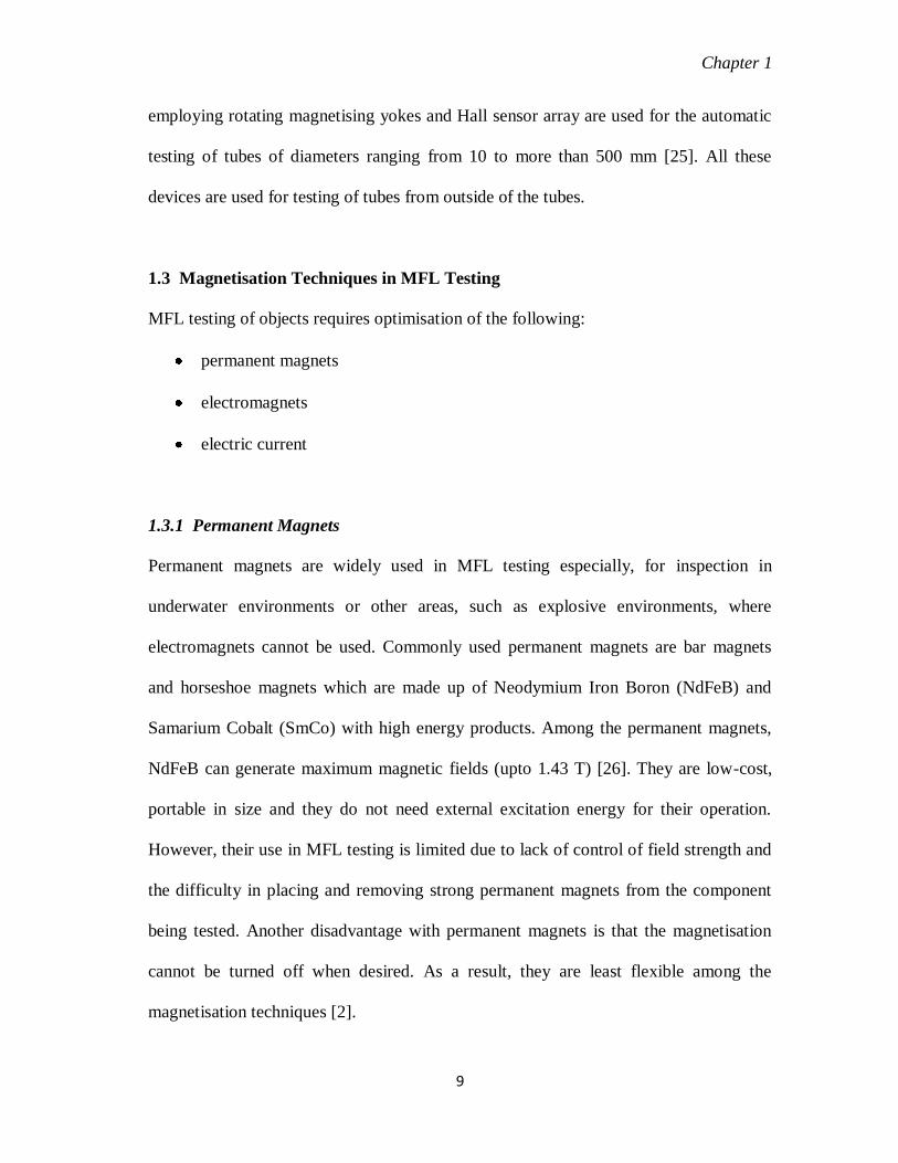
Permanent magnets are widely used in MFL testing especially, for inspection in
underwater environments or other areas, such as explosive environments, where
electromagnets cannot be used. Commonly used permanent magnets are bar magnets
and horseshoe magnets which are made up of Neodymium Iron Boron (NdFeB) and
Samarium Cobalt (SmCo) with high energy products. Among the permanent magnets,
NdFeB can generate maximum magnetic fields (upto 1.43 T) [26]. They are low-cost,
portable in size and they do not need external excitation energy for their operation.
However, their use in MFL testing is limited due to lack of control of field strength and
the difficulty in placing and removing strong permanent magnets from the component
being tested. Another disadvantage with permanent magnets is that the magnetisation
cannot be turned off when desired. As a result, they are least flexible among the
magnetisation techniques [2].

Chapter 1
10
1.3.2 Electromagnets
Several electromagnets such as electromagnetic yoke, solenoid and Helmholtz coils are
extensively used depending upon the geometry and accessibility of the components. The
magnitude of magnetising current can be varied so as to produce a wide range of
induced flux density required depending upon the thickness of the test component, size
and location of defects. Among the magnetisation techniques, electromagnets have the
most flexibility to suit the geometry of the test components. However, it is essential to
ensure good coupling with the component for better detection sensitivity and reliability
when electromagnets are used. The different types of electromagnets commonly used in
MFL testing are briefly discussed below:
1.3.2.1 Electromagnetic Yoke
Electromagnetic yoke consists of a soft iron C-core around which copper wire is
uniformly wound. A strong longitudinal magnetic field between the north and south
poles of the magnet is generated when electric current flows through the copper wire. A
typical electromagnetic yoke can generate magnetic field upto 2 T [27]. Yokes with
adjustable legs are commonly used in MFL testing for inspection of irregular shaped
components and welds [28]. A switch is generally included in the electrical circuit so
that the current and, therefore, the magnetisation can be turned on and off conveniently.
The yokes can be powered with alternating current from a wall socket or with a battery
pack.

Chapter 1
11
Suppose L, A and μ are the magnetic path length, area of cross-section and
relative permeability respectively of a specimen. Let N be the number of turns of copper
wire carrying a current I. Then, the total magnetic force in the magnetic circuit of a
yoke placed over the specimen with an air gap is given by [3],
(1.1)
where the subscripts represent the test specimen (s), core (c) of the yoke and air gap (a)
between the magnetising yoke and specimen surface. In ideal case where reluctances
of the core and air gap are both zero, the effective magnetic field Hs* in the test
specimen is given by,
(1.2)
Generally, industrial yokes are designed to provide at least 30-40 Oe
tangentially at the surface of the specimen, midway between the legs [3]. This region of
uniform surface field between the two legs can be checked by a gaussmeter. One
important aspect with yokes is heating of coil at prolonged use as well as due to use of
higher amperage.
1.3.2.2 Solenoid Coil
A solenoid is made by winding a large number of turns of insulated copper wire in a
helical fashion on an elongated former. Solenoids are often cylindrical in shape and
hence, they are suited for testing of cylindrical objects. When the length of a component
is several times larger than its diameter, an axial magnetic field can be established in the
component. If L is the length of the solenoid, D the diameter, I the current in the

Chapter 1
12
winding of N turns and x the distance from the centre of the solenoid, then the magnetic
field at x is given by [27]
(1.3)
At the centre of the solenoid x=0 and hence
(1.4)
For infinitely long (L is greater than at least 7 times the D) solenoid where L>>D
and , the above equation (1.4) reduces to
(1.5)
At the end of the solenoid, the field is equal to half the value of the solenoid at the
centre.
When a cylindrical component with considerable length is magnetised using a
solenoid, it is possible to obtain uniform axial magnetisation within and very near to the
solenoid and MFL sensor is placed in this region [27]. At some distance from the
solenoid, the magnetic lines of force will deviate from the axial direction and field
sensing sensors would not be usually placed in this region.
1.3.2.3 Helmholtz Coils
A pair of Helmholtz coils can also be used to generate a fairly uniform axial field over a
large volume of space in a component. They consist of two circular coils of the same
radius and number of turns on a common axis and separated by a distance equal to the
radius of the coil. The current flowing through the two coils of Helmholtz coils is in the
same direction. Let I be the current flowing in each coils of N turns and radius a

Chapter 1
13
separated by a. Then, the axial component of magnetic field intensity at an axial point
whose distance is x, is given by [3]
(1.6)
At the middle of the Helmholtz coils, the axial component of magnetic field
becomes
(1.7)
The radial component of magnetic field along axial direction is zero due to the
symmetry. The axial component of magnetic field close to the centre of Helmholtz coils
is also very weakly dependent on the radial distance from the axis. Therefore, the
magnetic field strength is maintained fairly constant over a large volume of space
between the two coils [3, 28]. The useful region of uniform field between the two coils
can also be increased by making the coil spacing slightly larger than their common
radius. Helmholtz coils are suited for magnetisation of cylindrical components.
1.3.3 Electric Current
Electric current can also be used for magnetisation of components through either
directly injecting current into the components or indirectly sending current to separate
conductors such as prods and central conductors. Various types of electric current
sources such as direct current (DC), alternating current (AC), half wave rectified current
(HWAC), etc. are used to obtain the required magnetisation of the part being inspected
[9]. The direction of electric current should be in such a way that the presence of a
discontinuity distorts the current flow as much as possible. Bars, billets and tubes are

Chapter 1
14
often magnetised with a direct electric current [2]. Prods, usually made from thick
copper, are used for weld testing. Central conductors are used for circumferential
magnetisation of hollow cylindrical tubes. The central conductors are usually solid
copper bars and they are placed inside the tube to generate circular magnetic fields.
In all the magnetisation techniques, it is necessary to ensure that the
magnetisation is perpendicular to the expected orientation of defects so as to get
maximum leakage field at the object surface.
1.4 Magnetic Field Sensors for MFL Testing
Commonly used magnetic field sensors in MFL testing are induction coils and Hall
sensors [29-31]. Coils measure the rate of change of a magnetic field, while Hall
sensors measure the actual magnetic field strength. SQUID (Superconducting Quantum
Interface Device) [32-33], anisotropic magneto-resistive (AMR) [34-35] and giant
magneto-resistive (GMR) [36-37] sensors are also found to use in MFL testing. The
characteristics and suitability of these magnetic sensors for MFL testing are discussed
below:
1.4.1 Induction Coils
Induction coils consist of some turns of insulated copper wire wrapped around a core.
When an induction coil is scanned across the defect, the magnetic flux linking with the
coil changes and a voltage is induced across the terminals of the coil. This output
voltage (E) is proportional to the number of turns (N) in the coil and the time rate of
change of flux (dφ/dt) linking with the coil as given below:

Chapter 1
15
(1.8)
where A is the cross-sectional area, B is the flux density and x is the distance moved by
the coil. Thus, the voltage induced in the coil is proportional to the gradient of flux
density along the direction of coil motion and the speed at which coil moves. Induction
coils are cheap, easy to manufacture and adaptable to any geometry. They do not
require any excitation and also not saturate even at quite large magnetic field levels [3].
But, they are less sensitive and possess poor resolution. They also require encapsulation
to minimize the eddy current effects.
1.4.2 Hall Sensors
Hall sensors are the most commonly used magnetic field sensors in MFL testing [38-
39]. The fabrication material of Hall sensors is specially grown semiconductor such as
indium arsenide, indium antimony, gallium arsenide or silicon. It works on the principle
of Hall Effect. When a current Ix carrying semiconductor is placed perpendicular to the
direction of an externally applied magnetic field Bz, a voltage VH will be generated
perpendicular to both the current and field given by
(1.9)
where RH is the Hall coefficient that depends upon the charge carriers and t is the
thickness of the semiconductor. Hall sensor measures the component of magnetic field
perpendicular to its chip plane. Typical sensitivity of Hall sensors are 100-600 mV/T
with excitation AC currents around 100 mA [40]. Their attractive features for MFL
testing include high linearity, small size, low-cost, operate at room temperature, and
possibility to fabricate sensor arrays for rapid inspection. Compared to induction coils,

Chapter 1
16
Hall sensors have very small active sensing area, so that they approximate to point
sensors [3]. However, they suffer from less sensitivity and large offset [41].
1.4.3 SQUID Sensors
SQUID (Superconducting Quantum Interface Device) sensor consists of a
superconducting ring closed by a Josephson junction. It works based on flux
quantization in superconducting rings and the Josephson Effect [42]. Among the
magnetic field sensors, SOUIDs has the highest sensitivity and can detect magnetic
fields of a few fT. It enables measurement of weak magnetic fields even without
applying a very large magnetising field [43]. It has the potential for detection of
discontinuities, material degradations in materials even at large lift-offs [44]. However,
it is necessary to use cryogenic liquid, generally liquid nitrogen and scan the cryostat to
get the signals, if the object can not be moved. Further, SQUIDs cannot be used for
applications in small diameter tubes.
1.4.4 AMR Sensors
Anisotropic magneto-resistance (AMR) sensors consist of thin ferromagnetic films (e.g.
permalloy) with a magnetic anisotropy. The application of an external magnetic field
will rotate the magnetisation with a resulting change in resistance. The resistance
changes roughly as the square of the cosine of the angle between the magnetisation and
the direction of current flow [34].The magneto-resistive (MR) ratio for AMR materials
is typically a few percent (3-4%) [45]. They have the advantages of less noise as

Chapter 1
17
compared to GMR sensors. However, their output may flip or reverse at higher
magnetic fields.
1.4.5 GMR Sensors
Giant magneto-resistance (GMR) is a quantum mechanical magneto-resistance effect
observed in a few nm thick multilayer structures such as Fe/Cr/Fe, Co/Cu/Co, etc. in
which ferromagnetic layers are separated by non-magnetic layers (Figure 1.4). The
Nobel Prize for the year 2007 in physics was awarded to Albert Fert and Peter Grünberg
for their discovery of GMR effect [46]. The GMR sensors work based on the GMR
effect in which there is a large change in electrical resistance to an applied magnetic
field due to the spin dependent scattering of electrons [47-48]. Ferromagnetic materials
have two types of electrons viz. spin up electrons and spin down electrons as carriers.
Spin up electrons are those electrons whose magnetic moments are parallel to the
direction of magnetisation of the material while spin down electrons have magnetic
moments antiparallel to the direction of magnetisation. The population of spin up
electrons is higher than the population of spin down electrons. It is more difficult for a
spin down electron to act as a carrier in the ferromagnetic film. This is the fundamental
reason for different surface scattering of spin up and spin down electrons of magnetic
materials used in GMR structures [49].
In order to exhibit the GMR effect, the mean free path of conduction electrons
has to greatly exceed the thickness of thin films. The mean free path of electrons in
many ferromagnetic alloys is on the order of 10 nm while the thickness of magnetic
films used in GMR structures is on the order of 5 nm. For such sufficiently thin films,

Chapter 1
18
surface scattering from the surfaces of the films plays the major role for higher
resistivity. It is also important that nonmagnetic film is lattice-matched to the magnetic
films so that electrons can pass from a magnetic film into the nonmagnetic film without
scattering. For example, Fe and Cr have the same crystal structure (body-centered
cubic) and similar lattice spacing.
When the magnetisations are antiparallel (Figure 1.4a), there is more scattering
i.e. the conduction electrons are not allowed to move freely and hence, they exhibit high
resistance. When an external magnetic field (leakage magnetic field for MFL testing) is
applied to this multilayer structure, the direction of magnetisation of the two magnetic
layers becomes parallel (Figure 1.4b) In this situation, there is less scattering resulting
to less resistance to conduction electrons. Since scattering has large effect on thin film
resistance, the difference in resistance for the two magnetic states can be relatively large
(Figure 1.5).
(a) (b)
Figure 1.4 GMR multilayer structures.

Chapter 1
19
Figure 1.5 GMR effect.
GMR sensors offer high sensitivity at low magnetic fields and high spatial
resolution [50-51]. Next to SQUID, GMR sensors are the most sensitive among the
magnetic field sensors. They can also be integrated as arrays to facilitate rapid scanning
of surfaces. But, they suffer from hysteresis effect and low saturation field. Table1.1
compares the performances of various magnetic field sensors used in MFL testing.
Table1.1 Comparison of commonly used sensors in MFL testing
Sensor Detectable
field range (T)
Sensitivity
(V/T)
Response
Time
Sensor
head size
Power
Consumption
Induction
coil
10 -4
- 10 3
0.25 0.1 MHz 2-10 mm 1 W
Hall 10 -6
- 10 2 0.65 1 MHz 10 -100 μm 10 mW
SQUID 10 -14
- 10 -6
104 1 MHz 10 -100 μm 10 mW
AMR 10 -5
- 10 0 2.5 1 MHz 10 -100 μm 10 mW
GMR 10 -12
- 10 -2
120 1 MHz 10 -100 μm 10 mW

Chapter 1
20
GMR sensors are found widespread use in eddy current NDE applications in
general [52-56] and for inspection of aging aerospace components, in particular [52-53].
Winchesky et al. [52] demonstrated the use of GMR sensors for the detection of deep
fatigue cracks and Yashan et al. [53] use GMR sensors for the detection of hidden
defects in a riveted aircraft structures. The GMR sensors can be used in eddy current
testing over a wide range of frequencies from DC to MHz [54]. Chomsuwan et al. [55]
used GMR based eddy current probe for inspection of Printed Circuit Boards (PCB).
Sasi et al. [56] developed EC-GMR sensor that could reliably detect corrosion attack at
8 mm below surface as compared to 4 mm achieved by the conventional EC probes.
GMR sensors are also found to use in MFL NDE applications [36, 57-59]. Using
the GMR sensor, Chen et al. [36] detected leakage magnetic fields from a 1.2 mm deep
(length, 10 mm and width, 10 mm) surface notch in a 12 mm thick oil pipeline. Yashan
et al. [57] used GMR sensors to detect small inclusions in thin steel sheets by MFL
technique. Kreutzbruck et al. [58] used GMR sensors for detection of real fatigue cracks
and artificial cracks of different depths and orientations in plates, bearings and rails.
Cracks with a depth of 40 μm could be resolved with a SNR of about 20. GMR sensors
are also useful for detection of stress and fatigue damage [59]. However, details on the
use of GMR sensors for detection of leakage fields from deep sub-surface defects are
scarce in the literature, although they find widespread use in eddy current testing.

Chapter 2
21
Chapter 2: Literature Review and Motivation
2.1 Literature Review
Historically, magnetic non-destructive testing was first started in 1868 at the Institute of
Naval Architects in England by Saxby [60]. He demonstrated the detection of defects
and other geometry irregularities in magnetised cannon tubes by making use of a
compass needle. In 1876, Hering was granted a patent for detection of discontinuities in
railroad rails by using similar technique [61]. The technique of magnetic particle testing
(MPT) was then developed by deForest [62] and Doane [63] around 1930. From then,
MPT became an important tool for non-destructive detection of defects in steels and
iron products. Later, as the subject of defect detection became more quantitative,
magnetic flux leakage (MFL) technique was derived from MPT by using field sensor,
instead of magnetic particles to enable the quantification of defects. The use of field
sensors for detecting leakage fields was first suggested in 1933 by Zuschlag [64]. The
use of sensor opened up new possibilities such as incorporation of latest advances in the
field sensing devices and associated signal and image processing techniques, modeling
of sensor response, etc. for enhancing the detection sensitivity of the existing MFL
techniques, especially for detection of deep sub-surface defects which is not possible by
MPT.
Several researchers [40, 65, 10] reported the state-of-art of NDE applications of
the MFL technique. The subject of MFL technique as an NDE tool had been extensively
reviewed by Beissner et al. [40]. They discussed the history of the development of the

Chapter 2
22
MFL technique, the underlying theory for the analysis of leakage field results to
characterize the defects and finally described its various applications for NDE of
ferromagnetic pipes, tubes, rods and round billets. Review of the subject of magnetic
leakage field calculations and interpretation of experimental measurements had been
reported by Dobmann [65]. He discussed the problem of sizing of defects in MFL
technique and attempted to solve it through an integral equation for field-defect
interaction. Jiles [10] reviewed the theoretical calculations of leakage fields and
applications of MFL technique for NDE of ferromagnetic tubes and pipes using
rotomat, tubomat and discomat systems.
The detailed literature review on modeling and experimental studies reported on
technique optimization, sensors and detectability for different components are given
below:
2.1.1 Modeling of MFL testing
One attractive facet of MFL technique is the ability to theoretically model the physical
phenomenon of leakage fields from defect region in a magnetised object. The modeling
enables the calculation of field-defect interactions and thus, helps better understanding
and more effective utilization of the MFL technique. The MFL modeling works
reported in the literature can be broadly classified into two categories:
Theoretical modeling
Numerical modeling

Chapter 2
23
2.1.1.1 Theoretical Modeling
Theoretical modeling of MFL technique is based on magnetic dipole method in which
defects are assumed as magnetic dipoles developed on the walls of the defect. Magnetic
moments of the dipoles are assumed opposite to the direction of the applied magnetic
field. These magnetic dipoles generate a magnetic field outside the specimen which is
equivalent to the leakage magnetic field. The theoretical modeling facilitates the
understanding of several properties of MFL fields. It has the advantages over numerical
modeling for offering a closed form solution, faster and convenient for simple
geometries [66-67].
The theoretical basis for modeling of MFL technique is discussed below:
In the absence of free current, the magnetic field intensity at any arbitrary point
is given by [40]
(2.1)
where the magnetic scalar potential satisfies the following integral equation
(2.2)
where is the magnetisation (dipole moment per unit volume) of the magnetised object
under test. The two terms on the right hand side of equation (2.2) correspond to two
distinct sources of MFL signals associated with a defect. The first term (integral over
the surface of object) is the induced surface magnetic charge density, ,
contributed due to the distribution of uncompensated magnetic poles on the defect
surface. The second term (integral over the volume of the object) is the induced volume
)(xH
x
)(x

Chapter 2
24
magnetic charge density, , arising due to variation in the permeability of the
test object near the defect.
Zatsepin and Shcherbinin [68] pioneered the dipole modeling of the MFL
technique for determination of leakage fields from two-dimensional (2D) surface-
breaking defects. They proposed that MFL signal arises from induced magnetic
polarization at the walls of a defect. They approximated 2D defects as line dipoles of
constant magnetic charge density and derived the expressions for tangential and normal
components of leakage magnetic fields due to the defect. Subsequently, Shcherbinin
and Pashagin [69-70] improved this model by considering three-dimensional (3D)
defects of rectangular cross-sections as surface dipoles. They also reported experimental
evidence that the surface magnetic charge density on the defect walls is not uniform
along the defect width. It is higher at the center of the walls than at the defect edges.
Shcherbinin and Pashagin [71] also studied the effect of the proximity of sub-surface
defects to the boundaries of the specimen on MFL fields.
Novikova and Miroshin [72] proposed that MFL signals are caused not only by
surface magnetic charge on the defect walls, but also by volume magnetic charge close
to the defect walls inside the bulk material. They approximated the volume magnetic
charge for a 2D defect with rectangular cross-section by a single filament of dipoles.
However, their theoretical equations are very complicated and modeling of real life
defects expected in components is difficult.
Förster [73-74] analysed the same types of defects but accounted for the
magnetic properties of the material and the applied magnetising field strength. The
practical significance of the different sections of magnetisation curve and hysteresis

Chapter 2
25
loop to the magnetic flux leakage was also studied. Based on the double dipole model,
Förster [74] proposed the approximate equations for tangential (Hx) and normal (Hz)
components of leakage field for a surface-breaking slot of a finite depth d in a linear
isotropic medium magnetised by a uniform magnetic field H0 as
(2.3)
(2.4)
The factor m is the induced dipole moment per unit length of slot given by
(2.5)
where w is the width of the slot and assumption is that the permeability (μ) of the
material is very much larger than that of air (μ0). The origin of the x-z co-ordinate axes
is at the centre of the top surface of the slot.
Using the idea of the Förster‟s dipole model and the image theory, Zhang et al.
[75] derived expressions for the Hx and Hz components of leakage field for a rectangular
defect (Figure 2.1) located at a depth h below the surface of the material magnetised by
a uniform magnetic field H0 as
(2.6)
(2.7)
where
(2.8)
(2.9)
Chapter 2
26
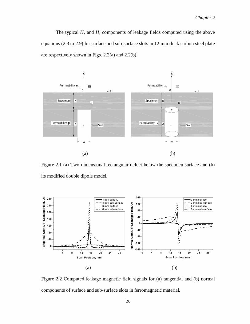
The typical Hx and Hz components of leakage fields computed using the above
equations (2.3 to 2.9) for surface and sub-surface slots in 12 mm thick carbon steel plate
are respectively shown in Figs. 2.2(a) and 2.2(b).
(a) (b)
Figure 2.1 (a) Two-dimensional rectangular defect below the specimen surface and (b)
its modified double dipole model.
(a) (b)
Figure 2.2 Computed leakage magnetic field signals for (a) tangential and (b) normal
components of surface and sub-surface slots in ferromagnetic material.
Specimen
Permeability
h
d
II
I Slot
w
Permeability
0 X
Y
III
Specimen
Permeability
h
d
II
I Slot
Permeability
0 X
Y
III
+
-
w
Z Z

Chapter 2
27
Edwards and Palmer [76] presented an analytical solution for the leakage field
of surface-breaking cracks. They considered variations in the dipole strength with the
magnetising conditions of the specimen. They showed that the relationships derived by
Zatsepin and Shcherbinin [66] for infinitely long cracks were also valid for finite
cracks, provided the magnetic leakage field was passed through the centre of the defect.
Minkov et al. [77-78] proposed that the surface magnetic charge density is not
uniform along the defect depth - it is higher at the defect tip compared to defect mouth.
They modeled this variation linearly. They also proposed a defect sizing scheme for
complex surface breaking cracks, based on the minimization of the root mean square
(RMS) error between the experimental Hall voltage measurement of leakage magnetic
field and theoretical dipole modeling of the crack.
Lukyanets et al. [79] solved an integral equation to derive asymptotic solution
for MFL signals from a single defect on the surface of a linear ferromagnetic half space
by approximating only one saddle point of Kernel. They proposed that the density of
defect-induced magnetic charges is directly related to the surface shape.
Mandache et al. [66] used the dipole model with constant surface magnetic
charge density to analyze MFL signals due to single defect and multiple cylindrical pit
defects situated close to each other. They used the locations of peaks of the normal
component of MFL signals along the center of the defect to determine the length of the
defect. The model result was also confirmed through comparison with experimental
MFL signals from different defect geometries.
Chapter 2
28
Dutta et al. [80-81] has recently proposed an analytical model by accounting the
variation of surface magnetic charge density for defect surfaces oblique to the direction
of applied field. The model was able to predict all the orthogonal components of 3D-
MFL fields of a surface-breaking defect [80]. They also proposed that the use of the
tangential (circumferential) component of MFL signal would be useful for
determination of location of defects with respect to the sensor [81].
The above literature review indicates that almost all the theoretical modeling
studies have been concentrated to the prediction of MFL signals from simple defect
geometries located at the object surface. They pose difficulties for realistic defect
shapes for most real life NDT problems and also lack generalization while making the
necessary assumptions to obtain tractable analytical solutions. Therefore, use of
theoretical modeling is limited for design of magnetisation systems and hence,
optimization of the MFL techniques for diverse applications including complex
geometries and defect shapes.
2.1.1.2 Numerical Modeling
Various numerical modeling methods have been reported for MFL NDE. They include
finite difference method (FDM) [82], finite element method (FEM) [83-84], boundary
element method (BEM) [85], hybrid method with FEM-BEM [86-87], meshless method
[88], etc. for analyzing MFL signals from defects in ferromagnetic components. Among
these, finite element (FE) method has been extensively used for study of leakage
magnetic fields in MFL testing as it can handle nonlinear [89], time-dependent and
circular geometry problems [90]. FE modeling has the advantages over theoretical

Chapter 2
29
modeling for enabling to model the complex boundary geometries and nonlinear
material characteristics found in actual defects and ferromagnetic materials. In general,
it requires intensive computer resources [91-92].
FE modeling of MFL technique was first carried out by Huang and Lord [93].
They could predict the field-defect interaction and this was a real breakthrough in the
area of MFL science and technology. This was followed by a series of significant works
by Lord et al. [94-95] and Atherton et al. [96-97]. The study showed that the FE
modeling has a potential tool for the design and optimization of MFL techniques
through analyzing MFL signals from defects [94-95]. In addition, it provides the
possibility of sizing of defects from the leakage field profile. Atherton et al. [97]
predicted the MFL signals from rectangular grooves of different depths in a pipe using
Infolytica MagNet software. In these early works, only 2D-FE modeling with
comparatively coarse mesh elements was employed and defects were treated as 2D
profile instead of the actual 3D geometry. However, since the MFL signals are
essentially three dimensional perturbations, 2D FE modeling of MFL technique appears
less satisfactory for signal calculations from real defects.
Ida et al. [98] realized a 3D-FE modeling to predict the leakage field around a
rectangular slot in a ferromagnetic bar. It could predict leakage fields of defects
regardless of their shape or location. Various groups [17, 34, 99-104] extended 3D-FE
modeling to study leakage fields for various test conditions. Naemi et al. [17] used
Infolytica MagNet software for modeling of MFL technique for inspection of
ferromagnetic plates and demonstrated that when modeling was extended to 3D, the
magnitude of the saturation magnetisation within the test plate was reduced. They

Chapter 2
30
compared the predicted MFL signals from 2D and 3D models and showed that a signal
obtained from 2D models is much larger than 3D models due to higher saturation level
in the area of the defect in 2D models. Zuoying et al. [99] and Ji et al. [100] used
ANSYS finite element software for 3D-FE modeling of pipeline MFL NDE to analyze
the influence of dimensions (length, width and depth) of surface defects and lift-off of
the sensor to the MFL signals. It was shown that the MFL signal amplitude increases
with the increase in width (Figure 2.3a) and depth of defects (Figure 2.3b) while the
MFL signal amplitude decreases with the increase in length of defects and lift-off of the
sensor. Ji et al. [100] also studied the influence of intensity of applied magnetic field on
MFL signals and observed that MFL signal amplitude increases initially with the
intensity of magnetisation and then tends to stable when the intensity reaches the
magnetic saturated condition. Chen et al. [101] performed 3D-FE modeling to
investigate the effect of complex corrosion on MFL signals from a 12 mm thick steel
plate and found that the relative positions of the complex corrosion pits affects the
magnitude of MFL signals. The effects of different pit corner geometries on MFL
signals were studied by Babbar et al. [102] and they reported that MFL signals are
influenced by the sharpness of the pit corner. The interaction between nearby corrosion
pits was studied by Mao et al. [103] using Infolytica MagNet 6 software and it was
found that the alignment of the pits had significant effects on the absolute values of
MFL signals. Li et al. [34] simulated 3D MFL signals from irregular shaped surface
defects in magnetic specimens using FEMLAB software and showed the potential for
improvement of defect characterization capabilities of existing MFL systems by sensing
all the 3D magnetic fields, especially for defects having irregular geometries. Ireland et

Chapter 2
31
al. [104] simulated a circumferential magnetizer for in-line inspection (ILI) of pipelines
under both static and moving tool conditions and highlighted the difficulties associated
with maintaining a stable magnetic circuit for a moving ILI tool.
(a) (b)
Figure 2.3 MFL signal peak-to-peak amplitudes (MFLpp) as functions of (a) defect
width (length 10 mm, depth 10 mm) in a 14 mm thick plate [99] and (b) defect depth
(length 10 mm, width 10 mm) in a 10 mm thick plate at various lift-offs [100].
Effect of velocity of MFL inspection tools (generally PIG) on MFL signals for
testing of pipelines was extensively studied using FE modeling by various groups [89,
91, 105-106]. Li et al. [89] used ANSOFT Maxwell EM V10 software and showed that
the shape and magnitude of the MFL signal changes with circumferential and axial
MFL and the velocity at which it influences the MFL signal is much lower in the
circumferential MFL than the axial MFL. Yang et al. [105] showed that the velocity-
induced circumferential fields of PIGs could be used for detecting axial stress corrosion
cracks in pipelines. Cui et al. [91] proposed a simplified FE modeling method to

Chapter 2
32
simulate the movement of MFL inspection tool inside the pipe in which the defect is
fixed and the magnetic fields along the axial direction are considered as representative
of the sensor signals from the MFL inspection tool.
Various group of researchers [107-110] paid significant scientific attention to
the effect of operating line pressure induced stress of the steel pipelines on MFL
signals. Leonard et al. [107] observed anisotropy on MFL signals, i.e., increase in MFL
signal amplitude along axial direction and decrease along circumferential direction of
pipes. Later, Ryu et al. [108] used Infolytica MagNet 6 software to investigate the
effects of local anisotropies simulating the stress concentrations induced by tensile
circumferential stress on MFL signals for various far- and near-side pit depths and they
observed that bulk stress and corrosion pit depth have a significant effect on MFL
signals. Babbar et al. [109-110] used Infolytica MagNet 6 software to analyze the
effects of dent-induced localized residual stresses [109] and dent geometry [110] on
MFL signals from a steel plate and found that the geometry effect signal is larger than
the stress effect signal. Further, they reported that the MFL signal has greater sensitivity
for compressive stresses than for tensile stresses.
Katoh et al. [28, 111] modeled the yoke magnetisation in MFL testing using 2D-
FEM and analyzed the influence of air gap between the magnetising yoke and specimen
and also specimen thickness on the detectability of flaw. They showed that MFL signal
decreases with the increase in air gap as well as specimen thickness [127]. They also
proposed an approach for estimation of intensity of magnetisation of the specimen by
extrapolating the intensity of magnetic field measured near the specimen surface to that
at lift-off being zero [28].
Chapter 2
33
In the last decade, researchers [26, 112-115] pursued FE modeling to optimize
the MFL techniques of tank floors [26] and pipelines [112-115]. Xiao-chun et al. [26]
used OPERA-3D finite element analysis software to research the influence of magnet
size (width, height, pole spacing), the air gap between the magnetic pole and specimen
surface and the magnetic force in the MFL testing of tank floors. The modeling results
indicated that variation of the magnet width affects the magnetisation much more than
variation of the magnet thickness and when the floor has reached its magnetising
saturation, the testing sensitivity and the SNR can improve with the increase in the
magnet-pole spacing and the pole-piece thickness. Park et al. [112-113] optimized the
magnetisation level of ferromagnetic pipes to obtain maximum change in leakage
magnetic flux from the region of defects. Their research found that the MFL signal
would be maximum if the magnetisation level is operated near to the saturation of B-H
curve [112] and the sensitivity of the optimized MFL system could also be increased to
200% by placing a high permeable back yoke system close to the sensor [113].
Mackintosh et al. [114] studied the various MFL assemblies for improving the detection
sensitivity in MFL testing of pipelines and obtained the highest improvement in the
MFL assembly when opposing magnetising assemblies were added to each end of the
primary magnetising assembly. Their result also indicated no improvement in the
sensitivity with the increase in magnet size and addition of brushes to the pole-pieces in
the traditional magnetising systems used in the pipeline testing. The research of Norouzi
et al. [115] for optimization of length of magnetising yoke used in MFL testing of
pipelines showed that longer yoke does not necessarily result uniform magnetic flux
density in the sample under test. The optimum length of the yoke was found to be

Chapter 2
34
between 300 mm to 400 mm for achieving higher sensitivity of defects in pipelines
(outer diameter 300 mm, wall thickness 10 mm).
In the above mentioned literature review, it is found that the majority of the studies
are focused on MFL signals under different defects shapes, dimensions and locations.
Effects of velocity of inspection tool and line pressure induced stress on MFL signals
for ILI of pipelines have also been thoroughly investigated. However, only few studies
have been carried out for the optimization of MFL techniques employed in pipes and
tank bottom floors. Therefore, a systematic numerical model based study is needed to
optimize the MFL techniques for various geometries used in different field applications.
2.2 Motivation
Although few modeling studies were reported for optimization of MFL techniques in
pipes and tank bottom floors, there is no systematic study to generalize the model based
optimization of the MFL techniques for different geometries. Apart from the pipelines
and tank bottom floors, ferromagnetic components such as carbon steel plates, stranded
track ropes, small diameter steam generator tubes, etc. are abundant in critical
applications. Corrosion induced defects are the major concerns in steel plates and tank
floors. Prolonged use of the ropes or wires is expected to cause abrasion and wear,
resulting in loss of metallic cross-sectional area (LMA) or localized flaw (LF) type
defects [21]. Detection of damage in the ropes or wires is essential as part of the
condition monitoring and life management programs. Periodic in-service inspection
(ISI) of steam generator tubes is essential to detect defects and size them [116]. NDE of
thick walled ferromagnetic tubes is challenging as the leakage magnetic field from outer

Chapter 2
35
surface defect is very feeble. There is a need to develop high sensitive, fast and reliable
NDE techniques for ISI of these critical components. As these components are made up
of ferromagnetic materials, MFL technique is well suited and the use of GMR sensors is
very attractive as they offer high sensitivity for low magnetic fields, good SNR and high
spatial resolution [36, 50].
For fast inspection of the components, array sensors are essential to facilitate
rapid scanning of the surfaces with large coverage. Further, optimization of MFL
techniques for these ferromagnetic components is inevitable for enhanced and reliable
detection of defects by increasing the MFL signal and at the same time, decreasing the
background noise. However, the detailed optimizations of magnetisation units for
various geometries, identification of number of sensors in an array and their optimal
locations are essential and general guidelines do not exist for various geometries.
Experimental based optimization is time consuming, cumbersome and sometimes,
impractical. In this context, the use of finite element numerical modeling is very
attractive.
2.3 Objective of the Thesis
The primary objective of the research work in the thesis is model based optimization
of MFL techniques for high sensitive, fast and reliable detection of defects in
ferromagnetic components in i) cuboid geometry, ii) solid cylindrical geometry and
iii) hollow cylindrical geometry. The scope involves optimization of the magnetisation
unit, number of GMR sensors and sensor locations for enhanced detection and fast
imaging of defects as detailed below:

Chapter 2
36
i) Optimization of GMR sensor based MFL technique for detection of shallow
surface defects and deep sub-surface defects in 12 mm thick carbon steel plates
(cuboid geometry)
ii) Optimization of GMR sensor based MFL technique for detection of localized
flaws and loss of metallic cross-sectional area type of defects in 64 mm outer
diameter steel ropes (solid cylindrical geometry)
iii) Optimization of GMR sensor based MFL technique for detection of localized
defects in 17.2 mm outer diameter (wall thickness, 2.3 mm) SG tubes of PFBR
(hollow cylindrical geometry).
The objective also includes proposing a generalized approach for model based
optimization of MFL technique for different geometries, based on the experience
gained from the studies on these three geometries.
2.4 Organization of the Thesis
The thesis consists of 9 chapters. The details of each chapter are summarized below:
Chapter 1 gives a brief introduction to MFL NDE and Chapter 2 provides a
comprehensive literature survey as well as objectives of the present work.
Chapter 3 deals with the details of 3D-FE modeling of the MFL technique. It
discusses the governing equations, boundary conditions applied, meshing and solver
used in the model. It explains the post processing of the FE solution for prediction of
MFL signal of a defect along the scan-line of the sensor at a definite lift-off.
Chapter 4 describes the optimization of GMR sensor based MFL technique for
detection of leakage magnetic fields from surface and sub-surface defects in cuboid

Chapter 2
37
geometry i.e. a ferromagnetic steel plate. It explains how the FE modeling has been
carried out to optimize the magnetising unit comprising of electromagnetic yoke for
achieving its optimum leg spacing, height and magnetising current used in the MFL
technique. Chapter 4 also discusses the influence of inclined and interacting defects
on MFL signals as well as the optimization of locations of 2D arrays of 16 GMR
sensors.
Chapter 5 describes the optimization of MFL technique for solid cylindrical
geometry i.e. steel track ropes, essentially optimization of two saddle coils based
magnetising unit and the development of a flexible GMR sensor array system.
Chapter 6 deals with the optimization of MFL technique for hollow cylindrical
geometry i.e. ferromagnetic SG tubes of PFBR. It explains the development of bobbin
coils and GMR tandem array sensors for imaging of localized defects in the tube.
Chapter 7 presents a generalized approach for model based optimization of
MFL technique for three different geometries. Application of this approach for various
geometries is discussed for fast and high sensitive detection of surface and sub-surface
defects in ferromagnetic materials.
The chapter 8 summarizes the major conclusions drawn from the model based
optimization studies as well as the experimental measurements. The chapter 9 gives
the scope for further studies.
Chapter 3
38
Chapter 3: Finite Element Modeling of MFL Technique
3.1 Introduction to Finite Element Modeling
The finite element modeling (FEM) is a numerical technique for finding approximate
solutions to boundary value problems. It was first proposed in the 1940s [117] and its
use began in the 1960s for structural and continuum mechanics and later found a wide
variety of applications in electromagnetic field problems [118]. Subsequently, FEM has
also been started using in NDE research community [119-120]. Today, the FEM has
become a general tool for designing many engineering devices to improve their
performances and efficiencies.
In FEM, the domain of interest is discretized into a finite number of sub-domains,
usually referred as elements. The interconnecting points are called nodes. The exact
variation of the unknown function (e.g. potential) is approximated by a simple
interpolation functions with unknown coefficients at each nodes associated with the
elements. In other words, the original boundary value problem with infinite degrees of
freedom is transformed into a problem with finite degrees of freedom. Then, a system of
algebraic equations is obtained by applying the Ritz variational or Galerkin procedure
and solution of the boundary value problem is obtained by solving the system of
equations. Finally, the desired parameters such as potential, field, etc. can be computed
at the nodes situated within the region of interest. The steps involved in the FEM of a
boundary value problem are as follows [117, 121]:

Chapter 3
39
1) Discretization of the domain
2) Selection of the interpolation functions
3) Formulation of the system of equations
4) Solution of the system of equations
5) Post-processing of the data
3.1.1 Discretization of Domain
Domain discretization is the most important step in any FEM as it affects the computer
storage requirements, the computation time and the accuracy of the modeling results. In
this step, the entire domain is divided into a finite number of sub-domains, usually
referred as elements. For one-dimensional (1D) modeling, the elements are often short
line segments interconnected to approximate the original line (Fig. 3.1a). For two-
dimensional (2D) modeling, the elements are usually small triangles and rectangles
(Fig. 3.1b). The rectangular elements are well suited for discretization of rectangular
geometry while, the triangular elements can be used for any geometries including the
irregular geometries. For three-dimensional (3D) modeling, the possible elements are
tetrahedral, triangular prisms and rectangular bricks (Fig. 3.1c). Among these,
tetrahedral are the simplest and best suited for arbitrary geometries [117].

Chapter 3
40
(a) (b)
(c)
Figure 3.1 (a) One-dimensional, (b) two-dimensional and (c) three-dimensional basic
finite elements.
3.1.2 Selection of Interpolation Functions
The second step of FEM is the selection of an interpolation function that approximates
the unknown function within an element. The interpolation is generally selected to be a
polynomial of first (linear), second (quadratic), or higher order. Higher order
polynomials are usually more accurate compared to lower order polynomials. However,
higher order polynomials result in a more complicated formulation than that of lower
order polynomials. Therefore, the simple linear interpolation is still widely used in the
FEM. The typical interpolation function of an element e at the node j in one dimension
is given by,
where a0 and a1 are unknown coefficients or parameters of the expansion and x is the
independent variable.

Chapter 3
41
3.1.3 Formulation of System of Equations
In this step, the elemental equation is first formulated using either the Ritz variational
method or Galerkin method. Then, all the elemental equations are assembled over all
elements to form the system of equations. Finally, the boundary conditions are imposed
to obtain the final form of the system of equations. There are two types of boundary
conditions viz. Dirichlet boundary condition and Neumann boundary condition.
Dirichlet boundary condition prescribes the unknown function at the boundary while the
Neumann boundary condition sets the normal derivative of the function to vanish at the
boundary.
3.1.4 Solution of System of Equations
In FEM, the system of equations is generally large set of algebraic equations. This set of
equations is then solved for getting the field or potential at the nodes. The different
formulations result in different matrices. These may be linear or nonlinear, sparse or
dense, symmetric or non-symmetric. If the system of equation is linear, it has been
solved using numerical linear algebra methods such as Gaussian elimination, LU
decomposition, QR decomposition, single value decomposition, Eigen value, etc.
Among these, Gauss elimination method is the most efficient method for solving a
linear system of equations, particularly if there is no special property of the matrix to
exploit (sparsity, symmetry, etc.). On the other hand, if the equation is nonlinear, it has
been solved using the Newton-Raphson method, Bailey‟s method, Chord method, etc.
[118, 122]. Depending upon the size of the system of equations, two types of solvers
viz. direct solver [123] and iterative solver [124] are available for solving the equations.

Chapter 3
42
Direct solvers are mostly used for solving relatively small size systems. It provides the
solution faster compared to iterative solver. However, for very large systems of
equations, the memory requirements of direct solvers are too large. Therefore, iterative
solvers are generally used in FEM. Iterative methods begin with an initial estimate for
the solution and successively improve it until it converges to the solution as accurate as
desired. In practice, the iteration terminates when some norm of the residual, or some
other measure of error, is as small as desired. Commonly used iterative methods for
solving systems of equations are conjugate gradient (CG), generalized minimum
residual (GMRES) and flexible generalized minimum residual (FGMRES) [118, 125].
The CG method is used only for symmetric positive definite matrices while GMRES
and FGMRES are used for general nonsymmetric problems. The GMRES method
computes a sequence of orthogonal vectors that minimizes the residual norm in a least
squares norm. Hence, the method leads to the smallest residual for a fixed number of
iterations. However, it requires preconditioners to improve the convergence. FGMRES
method can handle more general preconditioners which makes FGMRES method as the
more effective iterative solver in several FE modeling [125].
3.1.5 Post-processing of Data
Once the system of equations has been solved, we can compute the desired parameters
such as field or potential and display the results in the form of graphs or images which
are more meaningful and interpretable.

Chapter 3
43
3.2 Finite Element Modeling of MFL Technique
Finite element modeling has been extensively used for study of leakage magnetic fields
in MFL testing. It enables study of field-defect interactions and thus, helps in better
understanding of the MFL technique and enhances its applicability. FEM has the
advantages of flexibility for modeling of irregular material geometry and boundaries. It
yields a stable solution of required accuracy. It can also handle material nonlinearity
and eddy currents well. However, the representation of open boundaries is difficult. The
unknowns must be solved for throughout the whole domain even if the solution is
required only at a few points. It also requires intense computational time and resources
[118, 120]. Detailed literature review on FE modeling of MFL techniques for various
test conditions were discussed in Chapter 2. Here, the important steps needed for FE
modeling of MFL technique for various geometries are discussed.
3.2.1 Construction of Model Geometry
The first step in the FE modeling of MFL technique is to construct the model geometry.
The FE model geometry consists of the test specimen with defect, magnetisation unit
and a boundary black box. The typical geometry of 3D-FE model for MFL NDE of
carbon steel plate constructed using COMSOL Multiphysics package [125] is shown in
Figure 3.2. It consists of the steel plate with defect, electromagnetic yoke wounded with
copper coils and a boundary box.

Chapter 3
44
Figure 3.2. 3D-FE model geometry for MFL NDE of steel plate.
3.2.2 Mathematical Formulation
A complete description of the MFL phenomenon requires formulating both the
governing differential equation and boundary conditions. The governing equations
along with the boundary conditions imposed for FE modeling of MFL technique are
discussed in the following sub-sections:
3.2.2.1 Governing Equation
Maxwell‟s magneto-static equations given below are used for FE modeling of MFL
technique
(3.1)
(3.2)

Chapter 3
45
along with the constitutive relation
(3.3)
where B is the magnetic flux density,
H is the magnetic field intensity,
J is the current density,
μ0 is the magnetic permeability of free space,
μr is the relative permeability of the ferromagnetic material under test,
M is the magnetisation level of the material
The flux density B is related to the magnetic potential A as
(3.4)
Assuming the magnetic permeability of test material is isotropic, equation (3.2) can be
written as,
or, (3.5)
Here, is the source current density; , the eddy current generated by the applied
magnetic field and σϑ×(∇×A), the current density resulting from the relative motion
between the magnetizing unit (magnetic field) and the test specimen.
Equation (3.5) is the governing differential equation used in the FE modeling of MFL
technique. In this study, the effects of the eddy current and the motion of the
magnetizing unit are not considered.
In order to determine A uniquely in equation (3.5), Coulomb gauge condition as given
by [126] is imposed

Chapter 3
46
(3.6)
The solution to equation (3.5) can be obtained by minimizing the field energy related
expression called functional (Ritz variational formulation) given as
(3.7)
This can be written in terms of components of vector potential Ax, Ay and Az as,
(3.8)
The volume of the domain (boundary box) V is discretized into M small tetrahedral
volume elements. For an eth element of n nodes, the components of vector potential are
given by,
(3.9)
where is the shape function of the eth element. Substituting (3.9) into (3.8) gives the
value of F associated with the eth
element and by taking its partial derivatives, we get

Chapter 3
47
where the matrices and vectors are respectively given by,
and
Assembling of all the elements, the system of equations becomes
Minimizing the functional with respect to the components of vector potential, we obtain

Chapter 3
48
The system of equations can be written in the form of global matrix as,
(3.10)
or,
where is the [3N X 3N] global matrix (or stiffness matrix), is the (3N X 1)
unknown vector, is the (3N X 1) global source vector, and N is the number of nodal
points in the solution region [98].
At this stage, material properties such as magnetic permeability of the test
specimen, number of turns of copper winding, magnetisation current of the coil, etc. are
set for all the sub-domains used in the model. The next step is the application of
boundary conditions to the global system of equations.
3.2.2.2 Boundary Conditions
The magnetic insulation ( ) of Neumann boundary condition is applied to
boundaries (black box) confining a surrounding region of air. This sets the tangential
component of the magnetic potential or the normal component of the magnetic field to
zero [125]. Ideally, this condition is valid at infinitely large distances from the
specimen. However, in the interest of simplicity and computation time, the region of
interest is shrunk to a minimum subject to the condition that a significant increase in the
region of interest does not lead to any appreciable change in the spatial solution data.

Chapter 3
49
3.2.3 Meshing
Meshing is the discretization of the model geometry into small elements. For 3D-FE
modeling, the model geometry is discretized into tetrahedral mesh elements. The
number of mesh elements is determined from the shape of the geometry and element
order (linear, or of higher order) in the model. When the size of the elements is small, a
more accurate solution can be expected. On the other hand, it increases the number of
elements which leads to increase of the number of nodes and needs more computational
time to solve the resulting bigger global matrix. Hence, proper meshing should been
done wisely. One advantage of FEM is that meshing of various sizes can be done in
different sub-domains. A finer mesh must be used in the sub-domain where high
potential gradients (e.g. defect region) are expected. A courser meshing should be done
in the sub-domain of uniform potential. This will provide a more reliable and accurate
result in the reasonable computational time. If the meshing is refined further beyond a
certain limit, the accuracy of the solution will not improve further, due to round-off
errors associated with more number of computational operations for more number of
elements. One typical example of mesh that consists of 214584 tetrahedral elements
with corresponding 1380774 degrees of freedom is shown in Figure 3.3. The mesh
element size near the defect is chosen to be small (0.00002 m) to obtain an accurate
result in a reasonable computation time.

Chapter 3
50
Figure 3.3 Typical meshing for 3D-FE modeling of MFL technique of steel plate.
3.2.4 Solver
Equation (3.9) is solved in three dimensions using either direct or iterative methods. For
models with large degrees of freedom (more than 100,000), the direct solvers need too
much memory [125]. In such cases, the more memory-efficient iterative solvers such as
GMRES, FGMRES and CG perform better. However, iterative solvers are less stable
than direct solvers in that they do not always converge at a solution. For 3D-FE
modeling, the number of meshes and hence, the corresponding size of the system of
equations is reasonably large. Therefore, iterative method is generally employed for
solving the system of equations. Among the iterative solvers, FGMRES is more
effective with fast convergence. The computation time for solving equation (3.10) using
FGMRES solver is approximately 90 minutes in a dual core 64 bit processor with 8 GB
RAM workstation.

Chapter 3
51
3.2.5 Post-processing and Prediction of GMR Signal
Post-processing is performed to predict the desired parameters viz. magnetic flux
density B and field H from the magnetic vector potential A using the equations (3.4) and
(3.3) respectively. The flux density B is again post-processed to predict the Bx and Bz
components of the leakage flux from a defect along scan line of the sensor at a definite
lift-off. Various plotting methods such as surface, contour, streamline, etc. can be
performed for visualization of MFL profiles from the defects. The model predicted
MFL signals are further analyzed for design and optimization of the MFL techniques.
Typical magnetic flux density profiles of surface slot of 3.32 mm depth and sub-
surface slot located at 6.24 mm below the surface in a 12 mm thick carbon steel plate
are shown in Figure 3.4. One can easily visualize the leakage MFL profiles of the slots
from the arrow contour plots. As expected, the leakage magnetic field at the surface for
sub-surface slot is weaker than that of the surface slot.
(a) (b)
Figure 3.4 FE model predicted arrow contour plots for (a) surface slot of 3.32 mm depth
and (b) sub-surface slot located at 6.24 mm below the measurement surface.

Chapter 3
52
3.3 Validation of Model
COMSOL 4.3 Multiphysics software package has been used for optimization of MFL
techniques in the present thesis. Firstly, the model has been validated with the
experimental MFL signals. For this purpose, a hollow cylindrical geometry steam
generator tube (length 100 mm, outer diameter 17.2 mm and wall thickness 2.3 mm)
with circumferential notches (length 5 mm, width 1 mm) of depths 0.50 mm to 1.25 mm
in steps of 0.25 mm has been modeled. The tube has been magnetized with two bobbin
coils (cross-sectional area 10 x 3 mm2) wound on a ferrite core. Table 3.1 gives the
parameters used in the 3D-nonlinear FE modeling. The μr value of the tube is taken
from its magnetization curve as shown in Figure 3.5. Single GMR sensor positioned
centrally over the defects has been considered for modeling. Figure 3.6(a) shows the
comparison of model predicted and experimentally obtained (measured using a GMR
sensor) axial component of MFL signals (Ba) from the notches. A good agreement is
seen between the trends of model predicted and experimental MFL signal amplitudes.
Further, MFL signal peak amplitudes (Bapeak
) of notches have been calculated by
subtracting the background value (away from the notch) from the signal peak. In both
the cases, the Bapeak
amplitude increases with the increase in notch depth due to increase
in reluctance. The model predicted Bapeak
amplitude values are within 10% of the
experimental values. The deviation between the model and experimental values can be
attributed to the flux concentration intrinsically present in the GMR sensor.

Chapter 3
53
Table 3.1 Parameters used in the FE model
Bobbin coils No. of coils: 2
No. of turns of each coils: 70
Cross-sectional area: 10x3.4 mm 2
Current: 1.25 A
Conductivity: 5.98x10⁷ S/m
Ferrite core Length: 40.2 mm, Diameter: 4.8 mm
Relative permeability: 1000
Conductivity: 1.0x10⁻⁵
S/m
SG tube Length: 100 mm, Outer diameter: 17.2 mm
Wall thickness: 2.3 mm
Relative permeability: Magnetization curve
Conductivity: 4.03x10⁶ S/m
Defect (notch) modeled Length: 5 mm, Width: 1 mm, Depth: 0.50,
0.75, 1.00, 1.25 and 1.50 mm
Boundary condition assumed Magnetic insulation (n×A=0)
No. of mesh elements 255739
Size of mesh element at defect 0.00002 m
Degrees of freedom 1629568
Computation time 25 minutes in dual core 64 bit processor
workstation with 8 GB primary memory

Chapter 3
54
Figure 3.5 Magnetization curve for steam generator tube
(a) (b)
Figure 3.6 Comparison of model predicted and experimentally obtained (a) MFL signals
for circumferential notches and (b) its signal peak amplitudes

Chapter 4
55
Chapter 4: Optimization of MFL Technique for
Cuboid Geometry
4.1 Introduction
Ferromagnetic components of cuboid geometry are widely used in petrochemical and
refinery industries. Common examples are carbon steel plates and storage tank floors.
Carbon steel plates are also used in the flooring of above ground storage tanks (AST)
[17]. Corrosion related defects are of major concern for the carbon steel floors used in
these ASTs [127]. Defects can form on top and bottom surfaces of the tank floors. The
defects that form on the top surface are called surface defects or near-side defects while
the defects that form on the bottom surface are called sub-surface defects or far-side
defects. Prolonged corrosion and growth of defects can cause leak of hazardous
materials contained in the ASTs. Therefore, periodic inspection and maintenance of the
floors is essential. Among NDE techniques, MFL technique is widely used to detect
metal-loss defects or remaining wall thickness in the tank floors [20, 128-129]. This
particular application of MFL involves locally magnetising the floor plate and
measuring the leakage field just above the floor surface caused by a defect using
magnetic field sensors.
Ramirez et al. [129] carried out experimental studies using Hall sensors to
distinguish top and bottom defects of the tank floor and showed that there is a very high
similarity between MFL signals belonging to the top and bottom defects. They

Chapter 4
56
suggested that it is not viable to use standard MFL based techniques to discriminate top
and bottom defects. Liu et al. [20] studied the influence of specimen width on the local
magnetisation and showed that different areas of tank floors do not affect the testing
sensitivity, provided the thickness of the sample is same. Kasai et al. [14] used Hall
sensor to measure both Bx and Bz components of leakage fields from flat-bottomed holes
and rectangular grooves with various widths and depths in carbon steel plates of 12 mm
and 22 mm thickness. They proposed a practical procedure that uses linear relationship
between the MFL signal peak amplitude and defect cross-sectional area for determining
the depth of the flaw or residual plate thickness in storage tank floors.
Xiao-chun et al. [26] used OPERA-3D FE analysis software to study the
influence of permanent magnet size (width, height, pole spacing), the air gap between
the magnetic pole and specimen surface in the MFL testing of tank floors. The
modeling results indicated that variation of the magnet width affects the magnetisation
much more than the magnet height. Also, when the floor has reached its magnetic
saturation, the testing sensitivity and the SNR improve with the increase in the pole
spacing and height of the magnet. Validation experiments were performed using
permanent magnetic yoke and Hall sensors in 15 mm thick tank floors. Muzhitskii et al.
[130] discussed the problems in determining the optimum sizes of magnetising systems
based on permanent magnets as the strength of the magnetic fields depends on the size
of the magnet. However, detailed optimization of electromagnetic yoke based MFL
technique for cuboid geometry is still scarce and is required for enabling high sensitive
detection of defects. In all the above mentioned studies, Hall sensors are used for
detection of leakage magnetic fields from defects in cuboid shaped plates and floors.

Chapter 4
57
However, since the defects can occur on the top as well as bottom surfaces of the floor,
the sensitivity of the MFL technique employing Hall sensors is limited. In this context,
GMR sensors are attractive, especially for detection of deep sub-surface defects.
This chapter discusses the optimization of GMR based MFL technique for high
sensitive detection of surface and sub-surface defects in 12 mm thick carbon steel
plates. In order to optimize the structure of the electromagnetic yoke used in the
technique, 2D-FE modeling is performed. The number of GMR sensors and location of
2D GMR array sensors are optimized using 3D-FE model.
4.2 MFL Technique for Cuboid Geometry
The MFL technique proposed for cuboid geometry (steel plate) consists of a C-core
electromagnetic yoke, GMR array sensor, ferromagnetic plate with defects, X-Y
scanner, amplifier and personal computer. The yoke is used for uniform tangential
magnetisation of the plate. GMR array sensor is used to measure the Bx component of
the leakage magnetic flux by scanning the sensor array across the defect. The output
from sensors is amplified and digitized for analysis and interpretation.
4.3 Modeling
2D-FE modeling has been performed to optimize the magnetising unit comprising of an
electromagnetic yoke used in the MFL technique for cuboid geometry i.e. carbon steel
plate. Firstly, the structure of the electromagnetic yoke has been optimized for enhanced
detection of defects in the plate. Three different structures of C-core electromagnetic
yoke are possible for magnetisation of the steel plate as shown in Figure 4.1. Structure 1

Chapter 4
58
Excitation coil
Yoke
Sensor Defect
Plate
Yoke
Excitation coil
Sensor Defect
Plate
Yoke
Sensor Defect
Plate
Excitation coil
(Figure 4.1a) has one magnetising coil of 300 turns which is wound around the bow of
the yoke. Structure 2 (Figure 4.1b) has two symmetric coils, each of 150 turns which are
wound around the two legs of the yoke. Structure 3 (Figure 4.1c) has three coils- one
coil of 100 turns at the bow and two coils, each of 100 turns at the legs of the yoke. The
total number of turns in all the three structures is maintained the same i.e. 300 turns. In
order to detect both the surface and sub-surface defects and for optimization of the
yoke, 50% wall loss surface and sub-surface defects (6 mm deep in 12 mm thick plate)
have been considered. The Bx component of MFL signal at the sensor location has been
predicted for all the three structures and their peak amplitudes (Bxpeak
) have been
compared. The parameters used in the modeling are given in Table 4.1.
The following equation (4.1) has been solved in two dimensions using the FE
method:
(4.1)
where A is the magnetic vector potential, μr is the relative permeability and Ј is the
current density.
(a) Structure 1 (b) Structure 2 (c) Structure 3
Figure 4.1 Three different structures of C-core electromagnetic yoke for MFL NDE of
cuboid geometry.
sy
hy

Chapter 4
59
Table 4.1 Parameters used in the FE modeling of MFL technique for carbon steel plate.
Excitation coil No. of turns: 300
Cross-sectional area: 50x6 mm 2
Current: 4 A
Conductivity: 5.98x10⁷ S/m
Yoke Yoke height: 75 mm
Leg spacing: 75 mm
Relative permeability: 1000
Conductivity: 1.12x10⁷ S/m
Steel plate Dimensions: 240x12 mm 2
Relative permeability: B-H curve
Conductivity: 1.71x10⁷ S/m
Defect (groove) Dimensions: 1x6 mm 2
Boundary condition Magnetic insulation (n×A=0)
No. of mesh elements 43632
Size of mesh element at defect 0.0002 m
Degrees of freedom 88723
Solver MUMPS (direct solver)
Computation time 7.28 s in dual core 64 bit processor
workstation with 8 GB primary memory
The magnetic vector potential A is computed for the model geometry and the Bx
component of MFL signals for the surface and sub-surface grooves at different lift-offs

Chapter 4
60
are predicted. The model predicted contour lines of Bx component of magnetic flux
density for the surface groove for the three structures 1, 2 and 3 are shown in Figures
4.2(a), 4.2(b) and 4.2(c) respectively. Among the three structures, structure 1 has the
highest value of Bx as the direction of excitation coil is tangential resulting in higher
magnetic flux density of the excitation coil along the tangential direction. In structure 2,
the magnetic fields due to the excitation coils are mostly in the normal direction and
cancel each other at the middle of the two poles due to the symmetrical structure of the
excitation coils. Structure 3 has the magnetic fields in both the tangential and normal
directions, although the field is dominant along the normal direction. Figures 4.3(a) and
4.3(b) show the model predicted Bx component of MFL signals for the surface groove
and sub-surface groove respectively for the three yoke structures. The intensity of the
MFL signal is found to be highest in the structure 1 and lowest in the structure 2 for
both the defects. At the same time, the background magnetic field is also highest in the
structure 1 and lowest in the structure 2. As expected, the intensity of MFL signal for
the surface groove is higher compared to that of the sub-surface groove. However, the
MFL signal for the sub-surface groove is found to be broader than that of surface
groove due to divergence effect. The Bxpeak
amplitudes of both the surface and sub-
surface grooves for all the structures have been calculated and are shown in Figure 4.4.
The Bxpeak
amplitude is found to be highest in the structure 1 and lowest in the structure
2 for both the defects. This is attributed mainly to the tangential magnetisation of the
steel plate in the structure 1 meeting magnetic field lines perpendicular to the defect and
causing more leakage of magnetic fields from the defects. Moreover, the excitation coils
in the structures 2 and 3 are distributed against the localization of a single coil in the

Chapter 4
61
structure 1 leading to less resultant magnetic field of the component magnetic vector
fields due to the distributed coils in the structures 2 and 3. Therefore, structure 1 is
expected to provide the highest detection sensitivity. Hence, structure 1 has been chosen
as the optimum structure for magnetisation of the steel plates.
(a) Structure 1
(b) Structure 2

Chapter 4
62
(c) Structure 3
Figure 4.2 Model predicted contour lines of Bx component of magnetic flux density
from the surface groove for (a) structure 1, (b) structure 2 and (c) structure 3.
(a) (b)
Figure 4.3 Model predicted Bx component of MFL signals for (a) surface groove and (b)
sub-surface groove of the three yoke structures.

Chapter 4
63
Figure 4.4 Model predicted Bxpeak
amplitudes for surface and sub-surface grooves of the
three yoke structures.
4.3.1 Optimization of Yoke Height
Optimization of yoke height (hy) is important for enhanced detection of defects. The
height of the yoke is optimized using Bxpeak
amplitudes of the MFL signals of surface
and sub-surface grooves for different heights from 55 mm to 95 mm in steps of 10 mm
as shown in Figure 4.5(a). The Bxpeak
amplitude is found to decrease with the increase in
yoke height. This is attributed to the increase in length (L) of magnetic circuit with the
increase in yoke height which in turn, increases magnetic reluctance (R) given by
R=L/μ0μrA (A, being the cross sectional area of the yoke). The increase in magnetic
reluctance leads to reduction of magnetic flux (Ф=MMF/R, MMF being the
magnetomotive force which is equal to NI ampere-turns). However, the increase in
reluctance is very small as the permeability of the mild steel yoke is very high. As a
result, the Bxpeak
amplitude is found to be almost constant for all heights of the yoke and

Chapter 4
64
this observation is similar to that reported in [26]. Hence, a height of 75 mm has been
chosen as the height of the yoke.
(a) (b)
(c) (d)
Figure 4.5 Model predicted variation of Bxpeak
amplitudes with (a) height, (b) leg
spacing of yoke, (c) lift-off and (d) plate thickness for the surface and sub-surface
grooves.

Chapter 4
65
4.3.2 Optimization of Leg Spacing
The leg spacing (sy) of the yoke is optimized for obtaining uniform tangential
magnetisation of the plate between the two legs of the yoke so that sufficient detectable
magnetic fields are leaked out of the defects. The leg spacing is optimized using Bxpeak
amplitudes of the MFL signals of the surface and sub-surface grooves for different leg
spacing from 75 mm to 115 mm in steps of 10 mm as shown in Figure 4.5(b). The Bxpeak
amplitude of the MFL signal for surface groove is found to decrease with the increase in
leg spacing. This is primarily due to the increase in magnetic reluctance with the
increase in leg spacing of the yoke which leads to reduction in magnetic flux (and
hence, leakage magnetic flux) with the leg spacing. Similarly, the Bxpeak
amplitude of
the MFL signal for sub-surface groove is found to decrease with the leg spacing greater
than 95 mm. However, at smaller leg spacing (< 95 mm), signal amplitude of the sub-
surface groove is found to decrease due to less magnetic flux leading at the location of
sub-surface groove and limited space for leaking of distributed and broad MFL signal
from the sub-surface groove. Hence, a distance of 95 mm has been chosen as the
optimum leg spacing of the yoke for this technique, as it enables detection of both
surface and sub-surface defects. It also enables detection of leakage fields at higher lift-
offs (Figure 4.5c). However, the optimization of the leg spacing and hence the yoke
depends upon the thickness of the plate as shown in Figure 4.5(d). As can be seen, the
MFL signal peak amplitudes of both the surface and sub-surface grooves decrease with
the increase in plate thickness due to reduction in induced magnetic flux density with
the increase in plate thickness.

Chapter 4
66
4.3.3 Optimization of Magnetizing Current
The magnetising current is optimized for obtaining sufficient detectable leakage
magnetic fields from both the surface and sub-surface defects. Figure 4.6 shows the
model predicted Bxpeak
amplitudes of MFL signals as a function of magnetising current.
As can be seen, Bxpeak
increases with the increase in magnetising current and the rate of
increase of Bxpeak
amplitude decreases at higher currents following the non-linearity of
magnetization curve. However, at currents > 4 A there is a likelihood of saturation of
GMR sensor for leakage fields from deep surface-breaking notches. In view of this, 4 A
current is chosen as the optimum current in this study for detection of both surface and
sub-surface defects. Thus, the optimized magnetising unit for MFL NDE of 12 mm
thick steel plates is structure 1 with length 120 mm, width 50 mm, height 75 mm, leg
spacing 95 mm, winding 300 turns and magnetising current 4 A. Experimental
measurements have been made using this optimized magnetising yoke in this technique.
Figure 4.6 Model predicted Bxpeak
amplitudes of MFL signals as a function of
magnetising current.

Chapter 4
67
4.4 Experimental Setup
The schematic of the experimental setup used for the MFL measurements on a carbon
steel plate of cuboid geometry using the optimized yoke is shown in Figure 4.7. This
consists of a yoke, GMR sensor, ferromagnetic specimen with defects, X-Y scanner,
amplifier and personal computer. With electromagnetic yoke centered over the defects,
measurements are made by scanning the GMR sensor across the defects in steps of 0.2
mm. At sensor location, the Bx component (along the scan direction) of the leakage
magnetic flux is measured using the GMR sensor. The sensor output is first amplified
by a low noise amplifier consisting of a differential amplifier, a notch rejection filter at
50 Hz followed by a low-pass filter of 100 kHz and a single ended variable gain
amplifier with DC suppression for enhancing the signals. The variable gain amplifier is
set such that it amplifies the sensor output 8 times. This output is digitized using a DAQ
system of 16-bit A/D conversion card (PCI-1716) and then, stored in the computer for
subsequent analysis.
Figure 4.7 Schematic of experimental setup used for MFL measurements on carbon
steel plate.
Yoke
X-Y Scanner
DC Power Suppply
Amplifier
Computer
GMR
Sensor
Notch
Carbon Steel Plate
Controller

Chapter 4
68
For this study, GMR bridge sensors (AA003-02) manufactured by NVE
Associates are used. Because of the bridge circuit (Figure 4.8a), GMR sensor measures
the differential output voltage of the two sensing elements as a function of resistance
variation and ensures high stability with low noise. The GMR sensor has a maximum
hysteresis of 4% unit [51]. The output characteristic of the GMR sensor for calibrated
magnetic fields is shown in Figure 4.8(b). The sensitivity of the GMR sensor is found to
be 260 VT-1
at 5 V biasing voltage and the linear response is within the range of 0.2 mT
to 1.3 mT. This GMR sensor saturates at magnetic fields greater than 3 mT.
(a) (b)
Figure 4.8 (a) Functional block diagram of GMR bridge sensor and (b) GMR sensor
response characteristic.
4.5 Reference Defects
The specimens used in this study are five carbon steel plates (thickness, 12 mm) each
having two 15 mm long electro-discharge machining (EDM) notches of widths of 0.5
mm and 1 mm as shown in Figure 4.9 and of different depths (Table 4.2). With the
Pin 5, OUT +
Pin 1, OUT -Pin 4, V – (Ground)
Pin 3, V + (Supply)
GMRshield
shield
Functional Block Diagram

Chapter 4
69
notches on the GMR sensor side and on the opposite of sensor side (plate inverted),
surface (Figure 4.10a) and sub-surface notches (Figure 4.10b) are examined,
respectively. In the case of sub-surface notches, a definite location h below the scanning
surface exists for each notch. The physical lift-off between the GMR sensing layer and
the specimen surface is 0.3 mm.
Figure 4.9 Carbon steel plate specimen with EDM notches.
150 mm
450 mm
12 mm
15 m
m
Width, 0.5 mm Width, 1mm
150 mm 150 mm

Chapter 4
70
Table 4.2 Details of surface and sub-surface notches in 12 mm thick carbon steel plates
Plate
number
Notch type Length,
l (mm)
Width,
w (mm)
Depth,
d (mm)
Location below surface,
h (mm)
Plate 1 Surface 15 0.5 1.10 0
1 0.93 0
Sub-surface 15 0.5 1.10 10.90
1 0.93 11.07
Plate 2 Surface 15 0.5 1.74 0
1 1.72 0
Sub-surface 15 0.5 1.74 10.26
1 1.72 10.28
Plate 3 Surface 15
0.5 3.38 0
1 3.32 0
Sub-surface 15 0.5 3.38 8.62
1 3.32 8.68
Plate 4 Surface 15
0.5 5.84 0
1 5.76 0
Sub-surface 15 0.5 5.84 6.16
1 5.76 6.24
Plate 5 Surface 15
0.5 8.84 0
1 8.90 0
Sub-surface 15 0.5 8.84 3.16
1 8.90 3.10

Chapter 4
71
(a) (b)
Figure 4.10 Schematic showing (a) surface notch (near-side) and (b) sub-surface notch
(far-side).
4.6 Experimental Results
4.6.1 Surface Defects
The GMR sensor output for surface notches of different depths for two different widths
0.5 mm and 1 mm, after background removal are shown in Figures 4.11(a) and 4.11(b)
respectively. It can be seen that the GMR sensor detected all the surface notches and the
intensity of GMR sensor output increases with notch depth due to higher magnetic
reluctance from the deeper notches. However, when the notch depth increases beyond
5.84 mm, the leakage field becomes relatively insensitive to further increase in depth
and this observation is in agreement with that reported in [3]. This is more prominently
seen in Figure 4.11(a) in the case of 5.84 mm and 8.84 mm deep notches. With the
increase in depth, an increase in lateral spread of the MFL signals has been observed.
The amplitude of GMR signals from 0.93 mm deep (width 0.5 mm) and 1.1 deep (width
1.0 mm) surface notches are approximately 4 times the background signals from notch-
free regions.
Specimen
d Near - side Notch
w
Sensor
Specimenh
d I Far-side Notch
w
Sensor

Chapter 4
72
In order to assess the detection performance of the technique, signal and noise
amplitudes have been measured and the signal-to-noise ratio (SNR) is determined for all
the notches using SNR=20log(S/N), where S is the amplitude of MFL signal of a notch
and N is the amplitude of MFL signal in notch-free region (noise) of the plate. The SNR
of the shallowest notch (0.93 mm deep) is found to be 12.1 dB.
(a) (b)
Figure 4.11 GMR sensor signal output for various surface notches of (a) 0.5 mm width
and (b) 1.0 mm width.
The GMR sensor signal amplitude as a function of surface notch depth for two
different widths is shown in Figure 4.12. It is seen that the amplitude of MFL signal
increases with notch depth and notch width. The influence of notch depth is seen more
prominent than that of the notch width. The rate of increase in signal amplitude with
notch depth showed nearly two-slope behavior as depicted in Figure 4.12 (dotted line).
Larger slope is observed upto ~ 3 mm depth and thereafter, it is reduced. This reduction
in the slope at higher values of notch depth is due to the significant contribution of
induced volume magnetic charge density near the defect which leads to leakage of

Chapter 4
73
significant amount of magnetic flux to the other side of the plate. As expected, with
increasing width of notch, there is an increase in MFL signal amplitude.
Figure 4.12 GMR signal amplitude as a function of depth for surface notches (dotted
line shows the approximated two-slope behavior).
4.6.2 Sub-surface Defects
The GMR sensor output for sub-surface notches located at different depths for widths
0.5 mm and 1 mm are shown in Figures 4.13(a) and 4.13(b) respectively. It can be seen
that GMR sensor detected sub-surface notch located at 11.07 mm (depth 0.93 mm)
below the surface and this is a first time result. For this notch, the GMR signal is 3.92
times the background signal from the notch-free regions. This high sensitive detection
of deep sub-surface notch is possible due to the optimization of high sensitive GMR
sensor based MFL technique together with the low noise differential amplifier. The
GMR sensor signal amplitude as a function of notch location below the surface is
compared for two different notch widths and is shown in Figure 4.14. It can be observed

Chapter 4
74
that the leakage field strength is decreased with increase in notch location from the
surface and as a result, the amplitude of the MFL signal is decreased. Once again, two-
slope behavior is observed for the rate of decrease in signal amplitude with notch
location. The GMR sensor signal amplitudes are found to be higher for wider notches.
The lateral extent of signals is found to increase with increasing h due to the inherent
divergence effect. The lateral extent of the signals can be reduced by decreasing the leg
spacing of magnetising yoke (refer Figure 4.5b) and by increasing the magnetising
current (refer Figure 4.6) which will also increase the background noise. However, from
Figures 4.13 and 4.14, it is evident that resolution in depth and position evaluation
becomes poor when h increases.
(a)
0 10 20 30
0
50
100
150
Scan Position, mm
GM
R O
utp
ut,
mV
h=3.16 mmh=6.16 mmBackground
0 10 20 30
0
50
100
150
Scan Position, mm
GM
R O
utp
ut,
mV h=8.62 mm
Background
0 10 20 30
0
50
100
150
Scan Position, mm
GM
R O
utp
ut,
mV h=10.26 mm
Background
0 10 20 30
0
50
100
150
Scan Position, mm
GM
R O
utp
ut,
mV h=10.90 mm
Background

Chapter 4
75
(b)
Figure 4.13 GMR sensor signal response for sub-surface notches of (a) 0.5 mm width
and (b) 1.0 mm width located at different depths below surface.
Figure 4.14 GMR sensor signal amplitude for sub-surface notches as a function of notch
location below the surface.
0 10 20 30
0
50
100
150
200
Scan Position, mm
GM
R O
utp
ut,
mV h=3.10 mm
h=6.24 mmBackground
0 10 20 30
0
50
100
150
200
Scan Position, mm
GM
R O
utp
ut,
mV h=8.68 mm
Background
0 10 20 30
0
50
100
150
200
Scan Position, mm
GM
R O
utp
ut,
mV h=10.28 mm
Background
0 10 20 30
0
50
100
150
200
Scan Position, mmG
MR
Ou
tpu
t, m
V h=11.07 mmBackground

Chapter 4
76
4.6.3 Influence of Lift-off on MFL Signals
The influence of lift-off on the sensitivity of the MFL technique has been presented in
this section. The response of the GMR sensor with lift-off (lifting only the GMR sensor
from the plate surface) for sub-surface notches (length 15 mm, width 1 mm) located at
different depths below surface is shown in Figure 4.15. As can be observed, the GMR
sensor has detected all the notches upto 3 mm lift-off. At low lift-offs, the GMR signal
amplitude decreases drastically and then, it decreases gradually. Thus, this section
demonstrates that the optimized MFL technique can be used for non-contact and high
sensitive detection of surface and sub-surface defects in the plates.
Figure 4.15 Variation of GMR signal amplitude with lift-off for different sub-surface
notches in 12 mm thick carbon steel plates.
4.6.4 Influence of Inclined Defects on MFL Signals
The influence of inclined defects on the sensitivity of the MFL technique has also been
studied. Figure 4.16(a) shows the response of the GMR sensor for notches (length 15
mm, width 2 mm, depth 6 mm) of 0º, 15º, 30º and 60º inclinations. As expected, MFL

Chapter 4
77
signals are found to be asymmetric for inclined notches. The intensity of MFL signals
for the notches is found to decrease with increase in angle of inclination. Shift in signal
peak amplitude of MFL signals is also observed. In order to classify inclined or non-
inclined defects, the following nine parameters (shown in Figure 4.16b) are determined
from the measured MFL signals:
i) Difference in peak amplitudes (Bxlpeak
- Bxrpeak
)
ii) Full width at half maximum (FWHM)
iii) Rising slope
iv) Falling slope
v) Peak position
vi) Area under the signal
vii) Angle at signal peak
viii) Skewness and
ix) Kurtosis
In this study, the FWHM is taken as the full width at the half of the average peak
amplitudes of Bxlpeak
and Bxrpeak
. The Skewness and Kurtosis are defined as [131],
and
where μ is the mean and σ is the standard deviation of the distribution with variable x.
Figure 4.16(c) shows the variation of difference in peak amplitudes (Bxlpeak
-
Bxrpeak
) due to change in the inclination angle of the notches. It is observed that the

Chapter 4
78
asymmetry increases with the increase in angle of inclination. Skewness and kurtosis of
the MFL signals of inclined notches have been calculated and determined the
differential skewness and kurtosis with respect to the 0º inclination (non-inclined)
notch. Figure 4.16(d) shows the variation of differential skewness as a function of angle
of inclination of notches. As can be seen, the differential skewness increases with the
increase in angle of inclination. However, kurtosis shows very little change for small
angle of inclinations. Among the nine parameters, skewness has been found to be a
better parameter for classification of inclined or non-inclined defects. Thus, the
optimized MFL technique enables the sensitive detection of inclined defects through the
asymmetric behavior of MFL signals. This has been verified with the model prediction
which is discussed in the later section.
(a) (b)

Chapter 4
79
(c) (d)
Figure 4.16(a) Measured GMR sensor signal response for inclined notches, (b)
parameters determined from the measured MFL signals, (c) signal asymmetry and (d)
differential skewness as a function of angle of inclination of notches.
4.6.5 Influence of Interacting Defects on MFL Signals
Figure 4.17(a) shows the response of the GMR sensor for interacting notches (length 15
mm, width 1 mm, depth 6 mm) with notch-to-notch separations of 2.5 4, 6, and 8 mm.
As can be seen, the optimized MFL technique can resolve notches separated by a gap of
2.5 mm. The intensity of MFL signal decreases with the decrease in notch-to-notch
separation due to the effect of mutual interaction. The separation of peak positions are
nearly matching with the notch-to-notch separations. In order to distinguish interacting
defects from non-interacting defects, ratio of average Bxpeak
amplitudes of outer and
inner flanks has been calculated and the result is shown in Figure 4.17(b). At low
separations (2.5 mm and 4 mm), the notches are strongly interacting and then, it
interacts weakly. Finally, the notches are not interacting at 6.7 mm separations. This
observation is in agreement with the minimum of 5.6 mm times hole-to-hole separations

Chapter 4
80
measured at 1.5 mm lift-off using Hall sensors [132]. The variation is attributed to the
decrease in signal amplitude and hence less separations at higher lift-offs. Further, the
shape of Bx-Bz locus pattern is analyzed by measuring both Bx and Bz components of
magnetic flux from defects using two separate GMR sensors. Locus patterns are
observed to be distorted for interacting defects. Thus, the optimized MFL technique
enables the sensitive detection of interacting defects through the ratio of peak
amplitudes and distorted behavior of Bx-Bz locus pattern in MFL signals.
(a) (b)
Figure 4.17(a) Measured GMR sensor signal response for interacting notches and (b)
ratio of peak amplitudes of outer and inner flanks as a function of notch-to-notch
separations.
4.6.6 Validation
The model predicted characteristics of the MFL signals have been validated by
experiments using a GMR sensor scanned over the plate. The comparison of model
predicted and experimentally measured MFL signal amplitudes of sub-surface notches
as a function of notch location below the surface is shown in Figure 4.18(a). As can be

Chapter 4
81
seen, the MFL signal amplitude decreases with the increase in notch location below the
surface in both the cases. The rate of decrease in signal amplitudes with notch location
showed different slope beyond 6.24 mm (notch depth, 5.76 mm ~ 50% wall loss) as the
significant amount of flux is leaked to the other side of the plates. However, the
experimentally measured MFL signal amplitudes of notches with notch location beyond
6.24 mm are found to be larger than that of the model predicted signal amplitudes. The
difference in signal amplitudes beyond 6.24 mm location may be attributed to the
change in lift-off during experimental measurement.
(a) (b)
Figure 4.18 Comparison between the model and experimentally obtained (a) MFL
signal amplitude as a function of notch location below the surface for sub-surface
notches and (b) differential skewness as a function of angle of inclination for inclined
notches.
In the case of inclined defects, the model predicted and experimentally measured
differential skewness values as a function of angle of inclination are compared in Figure
4.18(b). In both the cases, differential skewness increases with the increase in angle of
inclination due to increase in asymmetry of MFL signals of inclined notches. Further,

Chapter 4
82
the differential skewness obtained from the experimental graph for 5º, 45º and 75º
inclinations are found to be 0.07, 0.68 and 1.31 respectively while the differential
skewness predicted from the 3D-FE model for 5º, 45º and 75º inclinations are 0.04, 0.61
and 1.39 respectively. At 5º inclination, the error for classification is 42% while, at 45º
and 75º inclinations, the errors are 10% and 6% respectively. Thus, the angle of
inclination (> 10º inclination) can be accurately classified using skewness.
4.7 Development of 2-dimensional GMR Array Sensors
For fast inspection of the carbon steel plates, sensing unit consisting of array sensors is
essential to facilitate rapid scanning of surfaces with the coverage of a large area of the
plate. Rigid 2D arrays of GMR sensors are attractive for fast inspection of the flat
surface plates. Further, optimization of the number of GMR elements and locations of
2D arrays between the two legs of the electromagnetic yoke is inevitable for enhanced
and reliable detection of defects. For optimization of the sensing unit, 3D-FE modeling
has been performed. Equation 4.1 with the magnetic insulation boundary condition has
been solved in three dimensions. The computation time for solving the equation 4.1
with 255528 numbers of tetrahedral elements is 21 minutes. Figure 4.19(a) shows the
model predicted surface plot of Bx component of the magnetic flux density between the
two legs of the yoke. As can be seen, the magnetic flux density is nearly uniform for an
optimum area of 60×25 mm2 (dotted region in Figure 4.19a).
The model predicted region can easily accommodate 16 GMR sensors. Hence, a
2D array of 4x4 GMR sensors has been fabricated (Figure 4.19b) and used for imaging
of defects in the plate. Each sensor element in the array has a common power input of

Chapter 4
83
5V, and the array has 16 differential outputs. The overall size of the sensor array is
20×17 mm2. The centre-to-centre distances (pitch) between two consecutive sensors
along the length and width directions are 5.5 mm and 4 mm respectively. The GMR
sensors measure the Bx component of leakage flux from defects in the plate. The output
from the array sensors is acquired and analyzed using a LabVIEW based data
acquisition system incorporating averaging and low pass filter to minimize noise.
(a) (b)
Figure 4.19 (a) Model predicted magnetic flux density between the legs of the
electromagnetic yoke (b) the photograph of fabricated 2D array of 4x4 GMR sensors.
The performance of the 2D array of 4x4 GMR sensors has been evaluated by
measuring the Bx component of leakage fields from surface defects in the plate. Figure
4.20(a) shows the typical output of the 16 element GMR array sensor scanned across a
notch (length 15 mm, width 1 mm and depth 3.32 mm). In Figure 4.20(a), we can see
the output of all the 16 GMR sensors. As expected, the output of GMR sensors is found
to be dependent on the position of the sensors. The GMR sensors output are processed
and MFL image of the notch is obtained as shown in Figure 4.20(b). As can be seen, it
20 mm
17 mm 60 mm length,
25 mm width
Yoke
Leg 1 Yoke
Leg 2

Chapter 4
84
is possible to obtain spatial information of the notch from the MFL image produced by
a single line scanning of the sensor array over the notch.
(a) (b)
Figure 4.20 (a) 16 element 2D GMR array sensor response for a 3.32 mm deep surface
notch and (b) its corresponding MFL image.
4.8 Conclusions
An MFL technique comprising of electromagnetic yoke and GMR array sensor
has been proposed for high sensitive detection of surface and sub-surface defects
in carbon steel plates of cuboid geometry. The structure of the magnetising yoke
and the important parameters such as leg spacing, height and magnetising
current of the yoke, number and location of GMR sensors used in the MFL
technique have been optimized.
The optimized technique is capable of detecting a shallow surface notch of 0.93
mm depth and a sub-surface notch located 11.07 mm below the measurement
surface in 12 mm thick plate.

Chapter 4
85
Two-slope behavior is observed for the rate of change in GMR sensor signal
amplitudes with notch depth for surface notches and notch location for sub-
surface notches.
The technique can be used for non-contact detection of surface and sub-surface
defects in the plates upto 3 mm lift-off.
Skewness has been found to be a better parameter for classification of inclined
or non-inclined notches. It can classify inclined (>10º inclination) notches with
an error of 10%.
The technique can resolve notches separated by a gap of 2.5 mm.
The model predicted features of the MFL signals have been experimentally
validated for a few cases.
A 2D array of 4x4 GMR sensors has been designed and fabricated for enabling
rapid detection and imaging of defects in the carbon steel plate.

Chapter 5
86
Chapter 5: Optimization of MFL Technique for Solid Cylindrical Geometry
5.1 Introduction
Ferromagnetic steel wire ropes of solid cylindrical geometry are widely used for
material handling in mines and hauling of men in ski-lift operations [2, 133]. In wire
ropes, two types of damage viz., local flaws (LF) and loss of metallic cross-sectional
area (LMA) occur mainly due to corrosion and wear [29, 134]. LFs are external and
internal discontinuities such as broken wires, cracks and corrosion pitting. Wire
breaking can occur due to fatigue, inter-strand nicking or martensitic embrittlement.
LMAs are distributed defects such as missing of wires caused by corrosion, abrasion
and wear resulting in loss of cross-sectional area. Periodic inspection of wire ropes is
important to ensure the structural integrity and to take corrective actions. Non-
destructive inspection of wire ropes is challenging due to their heterogeneous structure,
multiplicity, uncertainty of broken wires and hostile working environment.
Among various NDE techniques, visual and MFL techniques are widely used for
monitoring the health of steel wire ropes [135-136]. Although visual inspection is
simple and does not require special instrumentation, it is not suited for monitoring the
internal deterioration of ropes. On the contrary, the MFL technique is capable of
detecting both LF and LMA type defects in wire ropes [136]. In this particular
application of MFL technique, wire ropes are locally magnetised using electromagnets
or permanent magnets. If any defect is present in the rope, some amount of flux lines
leak out of the surface around the defect. This leakage flux is measured using magnetic
Chapter 5
87
field sensors and is correlated to the size and location of the defects. A variety of
procedures that use different types of sensors and magnetising devices have been
reported for reliable detection of defects in wire ropes [22-23, 137-138]. Wang et al.
[30] used flux gate sensors for detection of broken wires in a coal mine-hoist cable and
a back propagation neural network for assessment of the position and number of broken
wires in the cable. Jomdecha et al. [137] used printed circuit-shaped coils connected in
series as field sensors placed in a solenoid coil magnetisation and reported the detection
of 2 mm deep surface defects in a 38 mm diameter wire rope. Kalwa et al. [23, 138]
developed MFL systems with magnetic concentrators and Hall and coil sensors for
enhancing the detection sensitivity of defects in steel ropes. They suggested that
measurement of the axial component is more versatile than the radial component for the
detection of multiple defects in wire ropes.
One example of solid cylindrical geometry is track rope. Track ropes are a type
of wire ropes used for transportation of coal in mining industries. One such rope system
is operated for about 10 hours every day in Heavy Water Plant (HWP), Manuguru, to
transport 3000 tons of coal with the help of 256 numbers of buckets, each carrying
nearly 1.6 tons of coal. The track rope is stationary and is rigidly supported by towers at
periodic intervals. The schematic of the cross-section of the track rope along with the
design details is shown in Figure 5.1. The track rope has eight layers of stranded wires
of different diameters. The six inner layers are round-type wires, while the outer two
layers are Z-type wires. The round wires are locked by two Z wires to get the strength
of the rope. The width of the outer surface of the first Z wire is 6.45 mm, and the gap
width between two outer Z wires is 0.76 mm. During the operation of the rope system,

Chapter 5
88
the carriage wheels of the bucket come in contact with the top surface of the outer Z
wire as shown in Figure 5.2(a). Prolonged use of the rope system is expected to cause
abrasion and wear, resulting in LMA or LF type defects (Figure 5.2b). Also wire
breakage and formation of fatigue cracks, pitting corrosion, inter strand nicking or
martensitic embrittlement, etc. are likely to occur [21]. When more than two Z wires of
the outer layer are broken, they will be separated from the adjacent layers, as shown in
Figure 5.3. Therefore, detection of damage in track rope is essential to ensure the safety
and also to plan the replacement or repair of the track rope, as part of the condition
monitoring and life management programme.
This chapter discusses the model based optimization of MFL technique that uses
saddle coils and flexible GMR array sensor proposed, for the first time, for inspection of
artificial LFs and LMA defects in the 64 mm diameter steel track ropes.
Figure 5.1 The cross-section and design details of double locked track rope.
Layer Wire details Wire dia. or
thickness, mm
1 1 centre wire 4.00
2 6 round wires 4.66
3 6 filler wires 1.93
4 12 round wires 4.33
5 18 round wires 4.27
6 13 round wires 4.95
7 32 Z-wires 5.50
8 34 Z-wires 6.48
2 3
7
1
4
5
6
8
Z-wire
6.45 mm
Round
wire

Chapter 5
89
(a) (b)
Figure 5.2 (a) Photograph of the track rope system with bucket carrying coal and (b)
local flaws and loss of metallic cross-sectional area on the outer surface of the track
rope.
Figure 5.3 Breakage of wires at the outer surface of the track rope.
5.2 MFL Technique for Solid Cylindrical Geometry
An MFL technique that uses split-type saddle coils and flexible sensor arrays has been
proposed, for the first time, for the inspection of track ropes of solid cylindrical
geometry. Two saddle coils are used for uniform axial magnetisation of the rope. The
Loss of metallic cross-
sectional area Local flaws

Chapter 5
90
current in the saddle coils is set in opposite direction to enable predominantly axial
magnetisation of the rope region between the coils. A flexible GMR array sensor is used
to measure the axial (Ba) component of leakage magnetic flux by scanning the sensor
array and the magnetisation coils together as a single unit over the track rope. In order
to enhance the sensitivity, each GMR sensor output is amplified, digitized and stored in
the computer for subsequent analysis.
5.3 Modeling
Three different structures of coil based magnetising unit viz. solenoid, Helmholtz and
saddle coils are possible for magnetisation of the track rope as shown in Figure 5.4.
Among the structures, traditional solenoid (Figure 5.4a) and Helmholtz coil (Figure
5.4b) based magnetising units are not suited for practical field inspection as the
movement of the coil is obstructed by the supporting towers. On the contrary, split-type
saddle coils are convenient to move freely over the supporting towers. Moreover, most
of damages occur only on the top surface of the rope which can be easily covered by the
saddle coils. So, saddle coils (Figure 5.4c) based magnetisation unit has been chosen for
inspection of 64 mm diameter steel track ropes.
(a) Solenoid coil (b) Helmholtz coil (c) Saddle coils
Figure 5.4 Three different structures of coil based magnetising unit for MFL NDE of
track ropes.
Support Support Support
GMR
Track Rope Semicircular coils
Bias supply / Amplifier
Scan direction
Computer
DC power supply
0.05
Sensor
75 mm
30 mm
Rope Rope Rope ss

Chapter 5
91
5.3.1 Optimization of Magnetizing Current
3D-FE modeling has been performed to optimize the magnetising current
flowing in the two saddle coils and to predict the leakage magnetic fields from LFs and
LMA type defects in the track rope. Figure 5.5(a) shows the mesh generated for the
geometry which consists of a track rope (length 300 mm, outer diameter 64 mm) and
two saddle coils (length 120 mm, width 35 mm) each consisting of 90 turns with a cross
sectional area of 20 x10 mm2. Equation (5.1) has been solved in three dimensions using
the finite element method.
(5.1)
where A is the magnetic vector potential, μ0 is the magnetic permeability of free space,
μr is the relative permeability of steel and Ј is the current density.
For simplicity, in the model the track rope is assumed as a solid rod and GMR
sensor as well as velocity effects are not modeled. The magnetising current in the saddle
coils is taken as 5 A. Magnetic insulation (n×A=0) boundary condition is applied at the
outer boundaries of the model. The iterative solver is used for solving equation (5.1).
The computation time with 5673392 degrees of freedom is approximately 50 minutes
for a dual-core 64 bit processor workstation with 8 GB primary memory.
The magnetic vector potential A is computed in the solution region and the axial
component of the magnetic flux density between the two saddle coils is predicted.
Figures 5.5(b) and 5.5(c) are the model predicted magnetic flux line contours for same
and opposite directions of electric currents respectively. In the case of same direction of
magnetising current, the magnetic flux lines are predominantly along the radial
direction of the rope (Figure 5.5b). On the contrary, the magnetic flux lines are fairly

Chapter 5
92
uniform along axial direction of the rope for opposite direction of magnetising current
(Figure 5.5c). This is attributed to the same direction of electric current in the nearest
semicircular coils similar to the current direction in the Helmholtz coil. Hence, the
magnetising current in the saddle coils is set in opposite directions to ensure axial
magnetisation of the rope region between the saddle coils.
(a) (b) (c)
Figure 5.5 (a) 3D finite element mesh and model predicted magnetic flux line contours
between the two saddle coils for (b) same and (c) opposite directions of electric
currents.
The magnitude of magnetising current of the saddle coils is optimized for
obtaining sufficient detectable leakage field signals from all the flaws considered. The
current is optimized using the Bapeak
amplitudes of the MFL signals. The model
predicted Bapeak
amplitudes of the shallowest axial notch (2.05 mm deep) and
circumferential notch (1.94 mm deep) for different magnetising currents are shown in
Figure 5.6(a). As can be seen, Bapeak
increases with the increase in magnetizing current
Coil 1
(current
inward)
Coil 2
(current
outward
)
Coil 1
(current
inward)
Coil 2
(current
inward)

Chapter 5
93
for both notches due to higher magnetomotive force. However, there is likelihood of
saturation of GMR sensor at currents greater than 5 A. Hence, a current of 5 A has been
chosen as the optimum current for this technique.
5.3.1 Optimization of Inter-coil Spacing
The inter-coil spacing (ss) between the two saddle coils is optimized for
obtaining uniform axial magnetisation of the rope region between the two coils so that
sufficient detectable magnetic fields were leaked out of the notches. It is optimized
using Bapeak
amplitudes of the MFL signals for the notches. The typical Bapeak
amplitudes of the shallowest axial notch (2.05 mm deep) and circumferential notch
(1.94 mm deep) for various coil spacing of 60 mm to 85 mm in steps of 5 mm are
shown in Figure 5.6(b). The Bapeak
amplitudes of the MFL signals for both axial and
circumferential notches are found to increase upto 75 mm spacing. At distances greater
than 75 mm, the signal amplitudes are seen decreased due to reduction in magnetic field
strength with the increase in inter-coil spacing of coils. Hence, a distance of 75 mm has
been chosen as the optimum inter-coil spacing between the two saddle coils.

Chapter 5
94
(a) (b)
Figure 5.6 Optimization of (a) magnetising current and (c) inter-coil spacing between
the two saddle coils.
5.4 Experimental Setup
The experimental setup used for the MFL measurements on a track rope is shown in
Figure 5.7. It consists of two saddle coils, variable DC power supply, track rope, GMR
sensor, GMR field meter and a personal computer. Each saddle coil consists of 90 turns
with a cross sectional area of 20x10 mm2. The two saddle coils are separated by a gap
of 75 mm. The current in the coils is set in opposite direction to enable predominantly
axial magnetisation of the rope in the region between the coils. GMR bridge sensor
(AA003-02) is kept at the middle of the saddle coils.
Measurements are made by moving the GMR sensor and saddle coils together as
a single unit over the track rope in steps of 0.5 mm. A constant lift off of 0.3 mm is
maintained between the GMR sensor and the track rope to avoid physical damage to the
sensor. In order to enhance the sensitivity of GMR sensor, its output is amplified using
a low-noise amplifier consisting of a differential amplifier, notch rejection filter at 50

Chapter 5
95
Hz, 100 kHz low-pass filter and a single-ended variable gain amplifier. The variable
gain amplifier is set such that it amplifies the sensor output by a factor of 10. The
amplified GMR sensor output is digitized using a 2-channel data acquisition system (16
bit) and stored in the computer for further analysis.
Figure 5.7 Experimental setup for the MFL testing of track ropes.
5.5 Reference Defects
LFs are simulated by EDM notches introduced on the outer surface of the track rope.
Four axial notches (A, B, C, D) and four circumferential notches (E, F, G, H) of 5.5 mm
length, 2.0 mm width and of different depths are machined. A schematic of the type and
location of the notches is shown in Figure 5.8. The distance between the notches is
maintained at 80 mm, which is slightly more than the length of magnetisation unit (75
mm) to avoid the mutual interaction of leakage fields from notches. The depths of the
EDM notches measured using the replica technique are given in Table 5.1. One LMA-
type defect (length 42.0 mm, width 9.2 mm, depth 3.0 mm) is simulated by removing
the material from the outer surface of the Z-wire, and this depth is around 46.3% of the
Z-wire diameter.
Track Rope
GMR Field Meter/Amplifier
Servo Motor Saddle Coils
Coil
GMR Sensor

Chapter 5
96
Figure 5.8 Schematic of the track rope having axial and circumferential machined
artificial notches.
Table 5.1 Details of artificial EDM notches machined in the track rope (length 5.5 mm
and width 2.0 mm)
Notch Notch Orientation Notch Depth, mm
A Axial 2.05
B Axial 4.11
C Axial 5.86
D Axial 7.91
E Circumferential 1.94
F Circumferential 3.88
G Circumferential 5.90
H Circumferential 8.24
5.6 Experimental Results
5.6.1 Local Flaws
The MFL signals of axial notches viz. A, B, C and D in the track rope are shown in
Figure 5.9(a). The signal amplitude of the shallowest axial notch, A (2.05 mm deep) is
approximately 4.9 times the background noise from the stranded structure of the track
130 mm 80 mm 80 mm 80 mm 80 mm 80 mm 80 mm 80 mm 130 mm
A B C D E F G H
0 130 210 290 370 450 530 610 690 820 mm
64 mm
820 mm
6.45 mm 0.76 mm

Chapter 5
97
rope. The SNR for notch A is better than 14 dB. As can be observed, all the four axial
notches are detected by the technique with two distinct peaks correlated to the edges of
axial notches. Double peaks are seen in the signals of the axial notches due to the
extended nature of the axial notches.
The MFL signals of circumferential notches viz. E, F, G and H in the track rope
are shown in Figure 5.9(b). Once again, all four circumferential notches have been
clearly detected. The signal amplitude of the shallowest 1.94 mm-deep circumferential
notch, E is 7.5 times the background noise. The MFL signals of the circumferential
notches in Figure 5.9(b) are seen sharp with a single peak, which is in contrast to that
observed for the axial notches in Figure 5.9(a).
(a) (b)
Figure 5.9 MFL signals for (a) axial notches and (b) circumferential notches.
0 50 100 150 200 250 300-100
-50
0
50
100
150
200
250
300
DC
B
A
GM
R S
en
so
r O
utp
ut,
mV
Scan Distance, mm
Axial notches
0 50 100 150 200 250 300-200
-100
0
100
200
300
400
500
HG
F
E
GM
R S
en
so
r O
utp
ut,
mV
Scan Distance, mm
Circumferential notches

Chapter 5
98
Figure 5.10 FWHM and signal amplitude for axial and circumferential notches.
In order to evaluate the detection and sizing capability of the technique, the peak
amplitude and FWHM are determined for all the signals and the results are shown in
Figure 5.10. The FWHM is determined after the Gaussian fitting of the data. The error
in the determination of FWHM is ±0.1. In the case of the axial notches, the amplitude of
the MFL signals is found to increase with notch depth and the FWHM is found to be
nearly constant. In the case of the circumferential notches, the amplitude increases upto
the 5.90 mm deep notch and then decreases, while the FWHM remains nearly constant.
The decrease in the signal amplitude of notches deeper than outer diameter, i.e. 6.48
mm, is due to the penetration of a significant amount of magnetic flux into the inner
layers of the rope and not reaching the GMR sensor to be detected. The signal
amplitude is expected to be higher for a larger thickness of Z-wire and smaller diameter
of the rope. It is also observed that the amplitude of the circumferential notches is
nearly two times higher than that of the axial notches of similar depth. However, the
FWHM of circumferential notches is found to be nearly two times lower than that of the
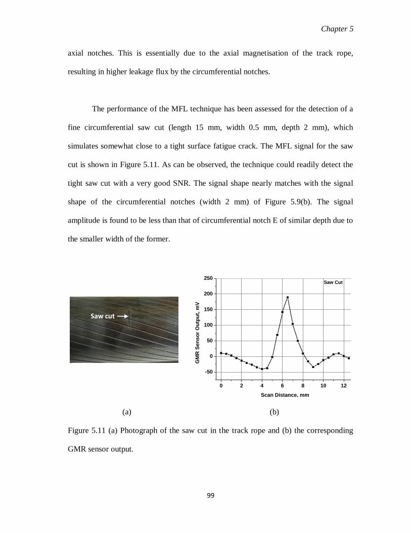
Chapter 5
99
axial notches. This is essentially due to the axial magnetisation of the track rope,
resulting in higher leakage flux by the circumferential notches.
The performance of the MFL technique has been assessed for the detection of a
fine circumferential saw cut (length 15 mm, width 0.5 mm, depth 2 mm), which
simulates somewhat close to a tight surface fatigue crack. The MFL signal for the saw
cut is shown in Figure 5.11. As can be observed, the technique could readily detect the
tight saw cut with a very good SNR. The signal shape nearly matches with the signal
shape of the circumferential notches (width 2 mm) of Figure 5.9(b). The signal
amplitude is found to be less than that of circumferential notch E of similar depth due to
the smaller width of the former.
(a) (b)
Figure 5.11 (a) Photograph of the saw cut in the track rope and (b) the corresponding
GMR sensor output.
0 2 4 6 8 10 12
-50
0
50
100
150
200
250
GM
R S
en
so
r O
utp
ut,
mV
Scan Distance, mm
Saw Cut
Saw cut

Chapter 5
100
0 10 20 30 40 50-100
-50
0
50
100
150
200
250
300
C5
C4
C3
C2
C1
GM
R S
en
so
r O
utp
ut,
mV
Scan Distance, mm
Multiple cuts
(a) (b)
Figure 5.12 (a) Photograph of 5 saw cuts separated by 13.5 mm, 10.0 mm, 5.5 and 3.2
mm distances and (b) the corresponding GMR sensor measured MFL signals.
Further, the resolution of the MFL technique has been evaluated by studying the
signals of five saw cuts (C1, C2, C3, C4 and C5), each of length 23.2 mm, width 1.0
mm and depth 2.0 mm, separated by finite distances as shown in Figure 5.12(a). The
MFL signals of the saw cuts are shown in Figure 5.12(b). It is found that the proposed
technique is able to detect all the 5 saw cuts. The intensity of the leakage field is found
to decrease with the decrease in separation between the saw cuts due to the effect of
mutual interaction. The MFL technique is able to clearly distinguish the saw cuts
separated by a gap of 3.2 mm. It may be noted here that a large variation in scanning
speed and lift-off during testing may change the signal amplitude and hence the
resolution of the technique.
C1 C2 C5 C3 C4

Chapter 5
101
5.6.2. Loss of Metallic Cross-sectional Area
The MFL signal of the simulated LMA (length 42.0 mm, width 9.2 mm and depth 3.0
mm) for scanning along the AA direction is shown in Figure 5.13. As can be observed,
the technique is able to detect unambiguously the LMA in the track rope with good
SNR. Following the dimension of the LMA, the MFL signal of LMA is found to be
extended compared to the sharp signal of the LF. The signal amplitude of LMA is found
to be 468.7 mV, which lies between the signal amplitude of circumferential and axial
LFs. The FWHM of LMA is found to be 29.1 mV, which is unambiguously more than
the FWHM of circumferential notches (~2.0 mm) and axial notches (~5.0 mm).
Figure 5.13 Photograph of LMA (42.0 mm length, 9.2 mm width and 3.0 mm depth)
machined in the track rope and its GMR sensor response scanned along dotted line AA
direction.
The proposed MFL technique can be used for condition monitoring of the track
rope as it enables reliable detection of LF and LMA type flaws on the outer layer of the
track rope. The high resolution of the technique is expected to enable effective detection
A A

Chapter 5
102
of degradation on the track rope during periodic inspection and can help in prevention
of premature retirement of track rope, through implementation of timely corrective
actions.
5.6.3 Validation
The MFL signals of LFs and LMA type defects have been predicted using the model.
Figure 5.14(a) shows the model predicted normalised MFL signals of the axial notch, C
and the circumferential notch, G (5.5 mm length and 2 mm width) of similar depth. The
MFL signals are normalised to the signal peak amplitude of the circumferential notch,
G. It is found that the signal amplitude of the notch G is found to be 2 times higher than
the notch C. However, FWHM of notch G is found to be 2 times lower than the notch
C, essentially due to the axial magnetisation of the track rope. Figure 5.14(b) shows the
MFL signals of notches C and G measured experimentally using a GMR sensor.
(a) (b)
Figure 5.14 (a) Model predicted MFL signals from the axial notch, C and the
circumferential notch, G and (b) the corresponding experimentally measured GMR
sensor response.

Chapter 5
103
The model predicted signal amplitude of the circumferential LFs is compared with the
experimentally obtained GMR signal amplitude in Figure 5.15(a). As can be seen, there
is an increase in signal amplitude in both the cases, except for the experimental signal
amplitude of the 8.24 mm deep notch. This attribute may be due to the fact that some of
the magnetic field lines are leaked into the second Z layer. It must be noted that the rope
is assumed as a single solid cylinder in the modeling, ignoring the noise arising from the
anisotropy of 0.76 mm wide helical Z layer strands which will be studied in future.
(a) (b)
Figure 5.15 Comparison of model predicted and experimentally measured (a)
normalised MFL signal amplitude of circumferential LFs and (b) MFL signal of LMA.
The model predicted normalised leakage field profile of LMA is compared with
the experimentally measured GMR output as shown along in Figure 5.15(b) and a good
agreement has been observed.

Chapter 5
104
5.6.4 Comparative Performance of Saddle Coils and Helmholtz Coil magnetisations
MFL signals of axial notches viz. A, B, C and D, obtained using Helmholtz coil
magnetisation (Figure 5.16) are shown in Figure 5.17(a). The GMR sensor output for
the shallowest axial notch, A (2.05 mm deep) is approximately 2.0 times the
background noise that comes mainly from 0.76 mm wide stranded structure of the track
rope. Similar to saddle coils magnetization (Figure 5.9a), all the four axial notches are
detected by the technique with two distinct peaks correlated to the edges of axial
notches. The signal amplitude in Helmholtz coil magnetisation is found to be ~ 4 times
higher than that of saddle coils magnetisation. It is due to larger uniform axial
magnetisation of the rope by the Helmholtz coil as compared to saddle coil
magnetisation and hence more leakage flux occurs from the notches. However, the SNR
of the shallowest axial notch, A (2.05 mm deep) for saddle coil (SNR=14 dB) is found
to be ~ 2 times higher than that of Helmholtz coil (SNR=6 dB). This is attributed to the
higher noise in the Helmholtz coil (only axial field) which arises due to stranded
structure of the rope as compared to saddle coil (both axial and radial fields). In the case
of Helmholtz coil magnetisation, both signal amplitude due to notch and noise
amplitude due to stranded structure in the rope are found to be higher. In the case of
saddle coil magnetisation, signal amplitude is found to decrease and the noise amplitude
is also found to decrease significantly.
MFL signals of circumferential notches viz. E, F, G, and H, obtained using
Helmholtz coil magnetisation are shown in Figure 5.17(b). Once again, all the four
notches are detected and the GMR sensor response of circumferential notches is found
to be sharp with a single peak as observed in the MFL signals using saddle coils

Chapter 5
105
magnetisation (Figure 5.9b). The signal amplitude of 1.94 mm deep notch, E is 3.2
times the background noise. The signal amplitude in Helmholtz coil magnetisation is ~
5 times higher than that of saddle coils magnetisation. However, the SNR of the
shallowest circumferential notch, E (1.94 mm deep) for saddle coil (SNR=18 dB) is
found to be ~ 2 times higher as compared to that of Helmholtz coil (SNR=10 dB). Also,
Helmholtz coil cannot be used for field inspection due to practical problems of
supporting towers whereas saddle coils can be used. Moreover, most of damages occur
only on the top surface of the rope which can be easily covered by the saddle coils.
Thus, saddle coils is found to be better than Helmholtz coil for inspection of track ropes
with half (top side) access.
Figure 5.16 Schematic of Helmholtz coil magnetisation based MFL testing setup.
GMR
Wire Rope
Helmholtz coil
Bias supply / Amplifier
Scan direction
Computer
DC power supply
0.05
Sensor
50 mm
20 mm
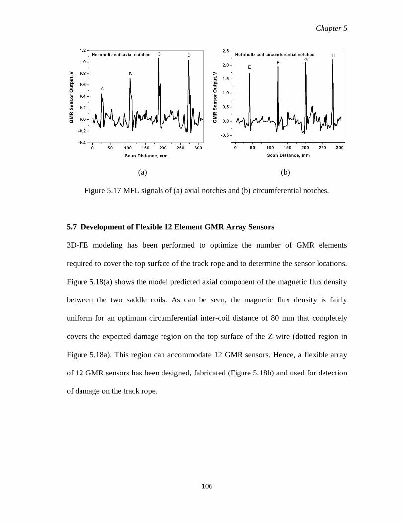
Chapter 5
106
(a) (b)
Figure 5.17 MFL signals of (a) axial notches and (b) circumferential notches.
5.7 Development of Flexible 12 Element GMR Array Sensors
3D-FE modeling has been performed to optimize the number of GMR elements
required to cover the top surface of the track rope and to determine the sensor locations.
Figure 5.18(a) shows the model predicted axial component of the magnetic flux density
between the two saddle coils. As can be seen, the magnetic flux density is fairly
uniform for an optimum circumferential inter-coil distance of 80 mm that completely
covers the expected damage region on the top surface of the Z-wire (dotted region in
Figure 5.18a). This region can accommodate 12 GMR sensors. Hence, a flexible array
of 12 GMR sensors has been designed, fabricated (Figure 5.18b) and used for detection
of damage on the track rope.

Chapter 5
107
(a) (b)
Figure 5.18 (a) Model predicted magnetic flux density between the saddle coils along
half of circumferential distance and (b) the fabricated flexible sensor array of 12 GMR
sensors.
The performance of the flexible 12 element GMR array sensors has been
evaluated by measuring the axial component of leakage fields from two LF and two
LMA type defects in track rope. The two LFs are simulated by EDM notches of size 5.5
x 2.0 x 2.0 mm3 (length x width x depth) oriented along axial and circumferential
directions in the track rope, as shown in photographs 5.19(a) and 5.19(b). The two
LMAs of sizes 42.0 x 9.0 x 3.0 mm3
and 33.5 x 14.2 x 4.9 mm3 are made along axial
and circumferential directions respectively (refer Figures 5.19c and 5.19d).
Coil 1
Coil 2

Chapter 5
108
(a) (b)
(c) (d)
Figure 5.19 Photographs of (a) axial LF, (b) circumferential LF, (c) axial LMA and (d)
circumferential LMA type defects in the track rope.
The MFL signals of the sensor array for the circumferential LF in the track rope
are shown in Figure 5.20. As the length of the flaw is 5.5 mm, only two GMR sensors
viz. S6 and S7 have shown the output of the leakage flux.
Figure 5.20 GMR sensor array response for a 5.5 mm long circumferential LF.
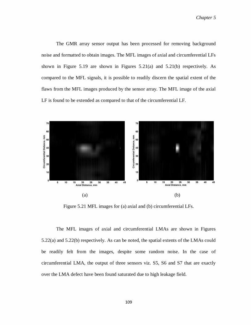
Chapter 5
109
The GMR array sensor output has been processed for removing background
noise and formatted to obtain images. The MFL images of axial and circumferential LFs
shown in Figure 5.19 are shown in Figures 5.21(a) and 5.21(b) respectively. As
compared to the MFL signals, it is possible to readily discern the spatial extent of the
flaws from the MFL images produced by the sensor array. The MFL image of the axial
LF is found to be extended as compared to that of the circumferential LF.
(a) (b)
Figure 5.21 MFL images for (a) axial and (b) circumferential LFs.
The MFL images of axial and circumferential LMAs are shown in Figures
5.22(a) and 5.22(b) respectively. As can be noted, the spatial extents of the LMAs could
be readily felt from the images, despite some random noise. In the case of
circumferential LMA, the output of three sensors viz. S5, S6 and S7 that are exactly
over the LMA defect have been found saturated due to high leakage field.

Chapter 5
110
(a) (b)
Figure 5.22 MFL images of (a) axial LMA (42.0 x 9.0 x 3.0 mm3) and (b)
circumferential LMA (33.5 x 14.2 x 4.9 mm3).
The flexible GMR sensor array has shown detection capability for both LF and
LMA type defects oriented along the axial as well as circumferential directions. The
sensor array has a fast detection speed along the length of the track rope and does not
require circumferential scanning. The images of circumferential notches have been
found to be sharp.
5.8 Conclusions
This chapter proposes, first of its kind, saddle coils-GMR based MFL technique for
condition monitoring of LF and LMA types of defects on the outer surface of 64
mm diameter steel track ropes.
The optimized technique is able to detect both LF and LMA type defects in track
ropes.

Chapter 5
111
2.0 mm deep axial and circumferential notches (length, 5.5 mm, width, 2.0 mm) in
the track rope are detected with SNR better than 14 dB.
The technique is able to resolve flaws separated by a distance of more than 3.2 mm.
Using the amplitude and FWHM of the MFL signals, it is possible to classify
whether the flaw in the track rope is axial or circumferential.
The model predicted characteristics of MFL signals for LF and LMA defects have
been experimentally validated.
A flexible 12 element GMR array sensor has been developed and used for fast
detection and imaging of both types of defects in the track rope.
The use of saddle coils-GMR array sensor based MFL technique is expected to
result in reliable periodic condition monitoring of the track rope, enhance safety and
incorporation of corrective measures that enable extension of life of the track ropes.

Chapter 6
112
Chapter 6: Optimization of MFL Technique for
Hollow Cylindrical Geometry
6.1 Introduction
MFL technique is widely used for inspection of hollow cylindrical geometry
components such as oil and gas transmission pipelines [15-16] and tubes [24-25]. About
80% of pipeline inspection is carried out using Pipe Inspection Gauge (PIG). A detailed
report has been submitted by Nestleroth et al. [15] for inspection of pipelines. MFL
technique can reliably detect metal loss due to corrosion and, sometimes, gouging
occurred in gas-pipelines. Apart from pipelines, small diameter ferromagnetic tubes are
abundant in critical applications. Some examples are steam generator (SG) tubes in
nuclear power plants and heat exchanger tubes in boiler and petrochemical industries.
The inspection of these tubes is extremely important to prevent catastrophic failures and
to extend their life. This chapter discusses the developmental study of MFL technique
for inspection of SG tubes of Prototype Fast Breeder Reactor (PFBR) of 500 MWe
being commissioned at Kalpakkam, India.
Steam generator is one of most critical components in sodium cooled PFBR.
The main function of SG is to extract the reactor heat through secondary circuit and
convert feed water into superheated steam in the tubes of SG. SG is a shell and tube,
once through vertical (height 25 m) heat exchanger (Figure 6.1a) with sodium on the
shell side and water on the tube side [139]. Any leakage in the sodium-water interface
would lead to catastrophic failure by violent sodium-water exothermic reaction which

Chapter 6
113
makes the SG a critical component in determining the efficient running of the plant.
Therefore, periodic ISI of SG tubes is essential to identify tube degradation at its
incipient stage and take remedial action to ensure safe and reliable operation of the
plant.
The structural material of SG tubes of PFBR is modified 9Cr-1Mo (Grade 91)
steel which is ferromagnetic. This material has been chosen in view of its excellent high
temperature creep and fatigue resistant properties and high thermal conductivity [140].
There are 547 tubes of outer diameter 17.2 mm and wall thickness (WT) 2.3 mm. Each
tube has an expansion bend of radius 375 mm to accommodate differential thermal
expansion. These tubes in the SG are stored as a bundle (Figure 6.1b) and generally
clamped outside the tube by Inconel-718 which is non-magnetic. Therefore, ISI of these
tubes is possible only from the inside of tube with limited accessible space. It should
also be noted that most of the degradation in ferromagnetic SG tubes takes place on the
outer surface of the tube, where they are more difficult to detect [141].
Figure 6.1 (a) Schematic of steam generator and (b) photograph of tube bundle
assembly.
2500
0
MANHOLE
BEND
EXPANSION
SODIUMOUTLET
INLET
SODIUM
MANHOLE
WATER
INLET
STEAM
OUTLET
(a)
(b)
Chapter 6
114
Several NDE techniques such as remote field eddy current (RFEC), partial
saturation eddy current (PSEC), MFL, internal rotary ultrasonic inspection (IRIS), etc.
are used for inspection of ferromagnetic heat exchanger tubes [2, 142-143]. The
working principles, advantages and limitations of these techniques were reported in [2,
142]. Among these techniques, RFEC technique is widely used for ISI of ferromagnetic
tubes due to equal sensitivity to both internal diameter (ID) and outer diameter (OD)
defects and does not require large space for placing the RFEC probes [143-144]. RFEC
technique is currently used for detection of defects in SG tubes of PFBR [116, 145].
Thirunavukkarasu et al. [116] showed detection of wall thinning of 10% WT, through
hole of 2 mm diameter and circumferential notch of 1.15 mm depth (50% WT) using
RFEC technique. This technique is capable of detecting uniform wall thinning and large
volumetric defects. However, it has shown that the RFEC technique has poor sensitivity
for the detection of localized cracks and shallow volumetric defects which are expected
to occur during service. Moreover, RFEC signals are influenced by the presence of
support structures and sodium deposits (non-magnetic and highly conducting) in the
defective regions of the tube which affects the sizing capability of the technique [145].
Therefore, a complimentary NDE technique to RFEC is essential for getting additional
information during ISI of SG tubes. Among the potential NDE techniques, MFL
technique is best suited for this purpose as it can detect both shallow surface and deep
sub-surface defects in ferromagnetic materials.
M. J. Bergander [146] reported MFL testing of ferromagnetic heat exchanger
tubes using permanent magnet for magnetisation and pair of induction coils for

Chapter 6
115
measurement of localized defects and gradual wall thinning in the tubes. Gotoh et al.
[147-148] proposed alternating MFL technique for inspection of outer side defects on
SUS 430 steel tube (OD 25 mm and WT 1.5 mm). They used an inner coil of low
frequency of about 60 Hz for excitation and a search coil for detection of defects and
showed detection of 0.5 mm (33% WT) deep circumferential defects. Krzywosz et al.
[149] used induction coils and Hall sensors to measure the leakage magnetic fields from
outer side erosion and holes in 19.05 mm OD carbon steel tube. They reported that
MFL testing is limited to a tubing size where ID is at least six times the nominal wall
thickness due to the physical constraints of the magnet size. Any inspection of tubes
exceeding the above criteria will result in reduced sensitivity, especially to OD flaws.
However, the ID (12.6 mm) of the SG tube in PFBR is about 5.5 times its wall thickness
(2.3 mm) which exceeds the above criteria. This demands the use of high sensitive
magnetic field sensors such as GMR sensors for detection of feeble magnetic fields
especially from outer side defects. Moreover, detail on the optimization of MFL
technique for small diameter tubes is scarce in the literature, although some details are
reported for large diameter pipelines [112-115].
This chapter presents the optimization of GMR based MFL technique, proposed
for detection of localized defects in small diameter (OD 17.2 mm) SG tubes of hollow
cylindrical geometry. The performance of the technique has been evaluated by
measuring the axial (Ba) component of leakage fields from localized outer side defects
in the SG tube. The details of the model based optimization of MFL technique and the
experimental measurement using GMR sensor are discussed.

Chapter 6
116
6.2 MFL Technique for Hollow Cylindrical Geometry
The schematic of the MFL technique proposed for inspection of small diameter SG
tubes of hollow cylindrical geometry is shown in Figure 6.2. It consists of two bobbin
coils, a variable DC power supply, tandem GMR array sensors, differential amplifiers
and a personal computer. The bobbin coils wound on a ferrite core is used for axial
magnetisation of the tube. The bobbin coils has the advantages over the permanent
magnet for allowing change in the magnetising current and also not adhering to the
tube. The use of ferrite core concentrates the magnetic field lines along central axis of
the tube and hence, reduces the compression of leakage fields due to direct magnetising
fields. In addition, the two ends of the ferrite core are attached with ferrite rings which
act as magnetic flux guiding device, by concentrating more magnetic field lines into the
tube. This enhances the sensitivity of leakage field from the defects in the small
diameter tube. The separation between the bobbin coils ensures predominantly uniform
axial magnetisation of the tube region between the two coils. Two tandem GMR array
sensors are kept at the middle of the bobbin coils with a phase shift as shown in Figure
6.2.

Chapter 6
117
Figure 6.2 MFL technique proposed for small diameter SG tubes of hollow cylindrical
geometry.
The axial component of the leakage flux from defects in the tube is measured
using the GMR array sensors by moving the GMR array sensors and magnetisation
coils together as a single unit inside the tube. In order to enhance the sensitivity of
GMR sensors, its outputs are filtered and amplified. The amplified GMR sensor outputs
are digitized and stored in the computer for subsequent analysis.
6.3 Modeling
2D-axis symmetry FE modeling has been performed to optimize the magnetising unit
comprising of two bobbin coils used in the MFL technique for hollow cylindrical
geometry i.e. SG tube. Firstly, the structure of the excitation coils has been optimized
for enhanced detection of defects in the tube. Three different core structures (Figure
6.3) of bobbin coils are considered for magnetisation of the SG tube. Structure 1 (Figure
PC based DAQ
25 mm
Excitation coils
Tandem GMRsensor arraysTube
Scan direction
Magnetizing current
Notch
PCB
GMR sensor arrayO/P voltage
0.05
GMR field meter/AmplifierDC power supply
SG Tube dimension:OD=17.2mm, ID=12.6mm, WT=2.3mm
Defect dimension (ID & OD):
Flat bottom hole - 2mm dia., 10%, 20% WL
Notch (Long. & Circum.) -10mm L, 0.5mm W, 0.25D)
Development of 8 GMR array sensor based MFL system for Non-destructive image and
evaluation of defects in steam generator tubes
5VDC
Ø17.2 mmFerrite core
GMR I/P supply
Ø12.6 mm
Flux guides

Chapter 6
118
6.3a) is the air core bobbin coils. Structure 2 (Figure 6.3b) is the ferrite core coils.
Structure 3 (Figure 6.3c) has extra flux guiding devices at the two ends of the ferrite
core. In order to detect both the ID and OD defects, ID and OD defects of 50% WT
(1.15 mm deep in 2.3 mm thick tube) have been considered for the optimization of the
magnetisation coils. The Ba component of MFL signal at the sensor location has been
predicted for all the three structures and compared their peak amplitudes (Bapeak
) for
obtaining the optimal structure.
(a) (b) (c)
Figure 6.3 Three different core structures of bobbin coils based magnetising unit for
MFL NDE of small diameter hollow cylinder.
The following equation (6.1) has been solved in two dimensions using the FE method:
(6.1)
where A is the magnetic vector potential, μr is the relative permeability and Ј is the
current density.

Chapter 6
119
Table 6.1 gives the parameters used in the modeling of MFL technique for SG tubes of
PFBR.
Table 6.1 Parameters used in the FE modeling of MFL technique.
Bobbin coils No. of coils: 2
No. of turns of each coils: 70
Cross-sectional area: 10x3.4 mm 2
Current: 1.25 A
Conductivity: 5.98x10⁷ S/m
Ferrite Length: 40.2 mm, Diameter: 4.8 mm
Relative permeability: 1000
Conductivity: 1.0x10⁻⁵
S/m
SG tube Length: 100 mm, Outer diameter: 17.2 mm
Wall thickness: 2.3 mm
Relative permeability: B-H loop
Conductivity: 4.03x10⁶ S/m
Defect (notch) Dimensions: 1x1.15 mm 2
Boundary condition Magnetic insulation (n×A=0)
No. of mesh elements 105748
Size of mesh element at defect 0.00002 m
Degrees of freedom 211591
Solver MUMPS (direct solver)
Computation time 24.43 s in dual core 64 bit processor
workstation with 8 GB primary memory

Chapter 6
120
The model predicted surface and normalised arrow plots of axial component of
leakage field from the OD notch for three different core structures of bobbin coils are
shown in Figures 6.4(a)-6.4(c). Among the three structures, ferrite core with flux guide
(Figure 6.4c) has the highest value of Ba in the tube as the magnetic field lines generated
by the two coils are drastically increased by the ferrite core together with the guiding of
magnetic field lines into the tube. The significant increase of the flux density has also
been seen in the surface plot (Figure 6.4c) of flux density of the ferrite with guide
structure as compared to that of flux density of the ferrite core alone. This is attributed
to the shorter magnetic path provided by the flux guide made up of ferrite. In the air
core structure (Figure 6.4a), the leakage magnetic flux from the notch is masked by the
direct magnetising field as the tube ID is very small (12.6 mm).
Figures 6.5(a) and 6.5(b) show the model predicted Ba component of MFL
signals for the ID notch and OD notch respectively at the sensor location for the three
core structures. The leakage magnetic fields from both the ID and OD notches are
clearly seen with the use of ferrite core as compared to the air core structure. This
observation is due to the concentration of magnetic field lines along the central axis of
the tube by the ferrite core and hence reduction of compression of leakage fields due to
direct magnetising fields. The intensity of the MFL signal is found to be highest in the
ferrite core with flux guide structure for both the notches. This can be clearly seen from
the Bapeak
amplitudes of the three core structures for both the notches (Figure 6.6). It can
be noted that the signal Bapeak
amplitude increases by 4 times with the use of flux guide,
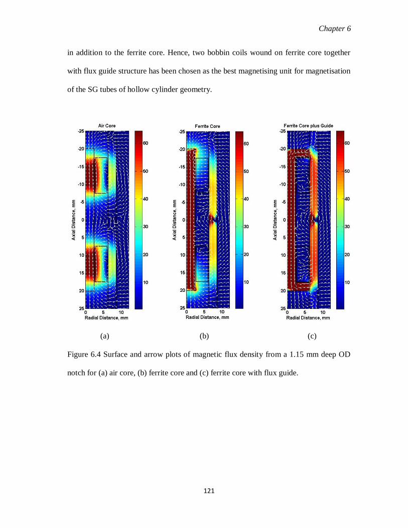
Chapter 6
121
in addition to the ferrite core. Hence, two bobbin coils wound on ferrite core together
with flux guide structure has been chosen as the best magnetising unit for magnetisation
of the SG tubes of hollow cylinder geometry.
(a) (b) (c)
Figure 6.4 Surface and arrow plots of magnetic flux density from a 1.15 mm deep OD
notch for (a) air core, (b) ferrite core and (c) ferrite core with flux guide.

Chapter 6
122
(d) (e) (f)
Figure 6.4 Surface and arrow plots of magnetic flux density from a 1.15 mm deep OD
notch (near defect) for (d) air core, (e) ferrite core and (f) ferrite core with flux guide.
(a) (b)
Figure 6.5 Model predicted Ba component of MFL signals for (a) ID notch and (b) OD
notch of three magnetising coil structures.

Chapter 6
123
Figure 6.6 Model predicted Bapeak
amplitudes of MFL signals for ID and OD notches of
three magnetising coil structures.
6.3.1 Optimization of Inter-coil Spacing
The inter-coil spacing (sc) between the two bobbin coils is optimized for obtaining
uniform axial magnetisation of the tube region between the two coils so that sufficient
detectable magnetic fields were leaked out of the notch. The axial component of leakage
fields is computed for various coil spacing of 15 mm to 40 mm in steps of 5 mm. The
inter-coil spacing is optimized using Bapeak
amplitudes of the MFL signals for both ID
and OD notches as shown in Figure 6.7(a). The Bapeak
amplitude of the MFL signal for
ID notch is found to decrease with the increase in inter-coil spacing. This is primarily
due to the reduction in magnetic field strength with the increase in inter-coil spacing of
the coils. On the other hand, the Bapeak
amplitude of the MFL signal for OD notch is
found to increase upto 25 mm spacing. At distances greater than 25 mm, the signal

Chapter 6
124
amplitude is seen decreased due to increase in magnetic reluctance with inter-coil
spacing. Hence, a distance of 25 mm has been chosen as the optimum inter-coil spacing
between the two bobbin coils for this technique.
(a) (b)
Figure 6.7 Optimization of (a) inter-coil spacing between the two bobbin coils and (b)
magnetising current.
6.3.2 Optimization of Magnetizing Current
The magnetising current is optimized to i) obtain sufficient detectable leakage magnetic
fields from all the notches considered in the study, ii) avoid the overheating of the coils
due to continuous current and iii) minimize the demagnetization requirement of the SG
tube. Figure 6.7(b) shows Bapeak
amplitudes of the MFL signals as a function of
magnetising current for both ID and OD notches. As can be seen, Bapeak
increases with
the increase in magnetising current for both notches and starts the saturation
magnetization of the SG tube at currents 5 A. However, the bobbin coils starts getting
heated up at currents greater than 2.5 A. In order to enable inspection of the SG tubes

Chapter 6
125
for a longer duration without cooling the coils and to minimize the demagnetization
requirement of the SG tube, the magnetizing current of 1.25 A is used. Experimental
measurements have been made using these optimized magnetising coils in this
technique.
6.4 Experimental Setup
The experimental setup used for the MFL measurements of SG tube using GMR sensor
is shown in Figure 6.8(a). It consists of two bobbin coils, a variable DC power supply, a
GMR sensor, a differential amplifier and a personal computer. The bobbin coils
consisting of two circular coils of 68 turns each separated by 25 mm is used for axial
magnetisation of the tube. The coil outer diameter is made 11.5 mm to fit inside the
tube. Each coil has cross-sectional area of 10 x 3 mm2 and wind on a 4.8 mm diameter
ferrite core. The ferrite core acts as a magnetic flux guiding device by concentrating the
magnetic field lines along central axis of the tube and hence, reduces the compression
of leakage fields due to direct magnetising fields. The GMR sensor is kept at the middle
of the bobbin coils as shown in Figure 6.8(b). The GMR bridge sensor (AAL002-02) is
used in this study. The axial component of the leakage flux from defects in the tube is
measured using the GMR sensor. Measurements are made by moving the GMR sensor
and magnetisation coils together as a single unit inside the tube with a speed of 2 cm/s.
A constant fill factor of 91.3% is maintained between the GMR sensor and the ID
surface of tube to avoid physical damage of the sensor. In order to enhance the
sensitivity of GMR sensor, its output is filtered and amplified 20 times using a low-

Chapter 6
126
noise differential amplifier. The amplified GMR sensor output is digitized using a 16 bit
DAQ system and stored in the computer for subsequent analysis.
(a)
(b)
Figure 6.8 (a) Experimental setup for MFL testing of SG tube and (b) photograph of
GMR sensor based MFL probe.
6.5 Reference Defects
The specimens used in this study are three straight SG tubes T1, T2 and T3 (length
1000 mm, OD 17.2 mm and WT 2.3 mm) with artificial reference defects. Localized
defects are simulated by notches and flat bottom holes (FBH) introduced on the outer
surface of the SG tubes T1 and T2 using EDM machining. Four circumferential notches
(A, B, C and D) of length 5 mm, width 1 mm and different depths are machined on the
outer side of tube T1. Four flat bottom holes (E, F, G and H) of diameter 2 mm and
different depths are machined on the outer side of tube T2. Four through holes (I, J, K
and L) of different diameters are also machined into the tube T3. The depths of EDM
notches and FBHs and diameters of through holes measured by replica technique are
given in Table 6.2.

Chapter 6
127
Table 6.2 Depths of reference defects in SG tubes
S. No. Tube No. Defect Defect type Defect depth/diam.,
mm
% Wall
thickness
1 T1 A Notch 0.54 23.65%
2 T1 B Notch 0.75 32.65%
3 T1 C Notch 1.19 51.83%
4 T1 D Notch 1.50 65.22%
5 T2 E FBH 0.22 09.57%
6 T2 F FBH 0.56 24.30%
7 T2 G FBH 1.14 49.70%
8 T2 H FBH 1.40 60.65%
9 T3 I Through hole 1.08 100%
10 T3 J Through hole 2.03 100%
11 T3 K Through hole 2.77 100%
12 T3 L Through hole 3.10 100%
6.6 Experimental Results
6.6.1 Localised Defects
The MFL signals of axial component of leakage fields of outer side circumferential
notches viz. A, B, C and D in the tube T1 measured by the GMR sensor, after
background removal, are shown in Figure 6.9(a). As can be observed, all the four
circumferential notches can be detected. The signal amplitude for the shallowest notch
A (0.54 mm deep, 23.65% WT) is approximately 2.9 times the background signals from

Chapter 6
128
notch-free regions. The SNR of the shallowest notch A (0.54 mm deep, 23.65% WT) is
found to be 9.2 dB. As expected, the signal amplitude is found to increase with the
increase in notch depth.
The MFL signals of axial component of leakage fields of flat bottom holes viz.
E, F, G and H in the tube T2 are shown in Figure 6.9(b). The technique detected three
FBHs F, G and H, except the shallowest FBH, E (0.22 mm deep, 9.57% WT). The
signal amplitude of the hole, F (0.56 mm deep, 24.30% WT) in the tube is
approximately 1.8 times the background signals from defect-free regions and its SNR
turns out to be 5.1 dB. Thus, the optimization of the MFL technique together with the
use of GMR sensors and differential amplifier enables to lower the minimum detectable
depth from 40% WT hole in 2.77 mm thick ferromagnetic carbon steel tube [142] to
24% WT hole in 2.3 mm thick ferromagnetic SG tube in MFL technique. The signal
amplitude increases with the increase in depth of holes.
The MFL signals of axial component of leakage fields of through holes viz. I, J,
K and L in the tube T3, after background removal, are shown in Figure 6.9(c). Once
again, the technique detected all the four holes. The SNR of the smallest hole, I
(diameter 1.04 mm) in the tube is found to be approximately 6.8 dB.

Chapter 6
129
Figure 6.9 GMR sensor response for outer side (a) EDM circumferential notches, (b)
flat bottom holes and (c) through holes in SG tube.
(a) (b)
(c)

Chapter 6
130
Figure 6.10 GMR sensor signal amplitude as a function of volume of defects.
In order to compare the detection sensitivity of the MFL technique for the three
types of defects viz. notches, FBHs and through holes, peak amplitudes of MFL signals
have been determined by taking the difference of peak and valley of MFL signals. The
peak amplitudes of MFL signals of the three types of defects are plotted as a function of
volume of defects, as shown in Figure 6.10. The peak amplitude increases almost
linearly with increase in volume of defect in all type of defects. Among the three types
of defects, the peak amplitude of through holes is found to be maximum for the similar
volume of defects. This observation is attributed to the higher reluctance with 100%
WT in through holes compared to the notches and FBHs and the MFL signal amplitude
depends upon more on depth as compared to length and width of defects [100].
The optimized GMR based MFL technique can be used for ISI of the SG tubes
as it enables reliable detection of OD defects in the SG tube. It is expected that the

Chapter 6
131
technique will detect ID defects with larger signals than OD defects as the field strength
on the ID side is higher than OD side. The use of GMR sensors with low noise
differential amplifier also enables to lower the minimum detectable depth of defects in
tubes with lower IDT ratio that were previously considered undetectable. The technique
does not require full saturation of the tube unlike in saturation eddy current technique.
The instrumentation is less expensive and much simpler as compared to RFEC
technique [146]. The high sensitivity of the technique is expected to enable effective
detection of both ID and OD defects in small diameter ferromagnetic tubes.
6.6.2 Influence of Support Plate on MFL Signals
The influence of support plate (Figure 6.11a) on MFL signal has also been analyzed.
Figure 6.11(b) shows the MFL signals of the 1.08 mm diameter hole with and without
the support plate. As can be seen, the MFL signals of holes are not significantly
influenced by the presence of support plate outside the SG tube. To verify the
experimental observation, FE modeling has been carried out simulating the situation.
Model predicted MFL signals of the hole with and without support plate is plotted
together with the experimental result in Figure 6.11(b). As can be seen, there is a good
agreement between the model predicted and experimental MFL signals. In both cases,
no significant change in the MFL signals is observed by the presence of support plate.
This is attributed to the non-magnetic (μr = 1.001) behavior of the Inconel-718 support
plate resulting similar field contour lines in the tube with and without plate as shown in
Figure 6.12(a) and 6.12(b) respectively. It can also be expected that the electrically
conductive non-magnetic sodium deposits, if present, in the defective regions of the SG

Chapter 6
132
tubes will also not influence the defect sensitivity of the technique. This will avoid the
use of multi-frequency excitation and associated signal and image processing
techniques to remove the influence of support plate and sodium deposits on RFEC
signals [112, 145]. Further, the MFL technique can be advantageously used to identify
the support plate and sodium deposits by comparing to RFEC signals.
(a) (b)
Figure 6.11 (a) Photograph of the SG tube with support plate (Inconel-718) and (b)
comparison of experimentally obtained and model predicted MFL signals for a 1.08 mm
diameter hole in tube with and without the support plate.

Chapter 6
133
(a) (b)
Figure 6.12 Model predicted contour plots of magnetic flux density (a) with and (b)
without the support plate.
6.6.3 Validation
The experimental MFL signals have been validated with the model predicted MFL
signals. The experimentally obtained GMR signal amplitude of the circumferential
notches (length 5 mm, width 1 mm and depths 0.54, 0.75, 1.19 and 1.50 mm) is
compared with the model predicted signal amplitudes in Figure 6.13. A good agreement
is seen between the trends of model predicted and experimental MFL signal amplitudes.
In both the cases, the Bapeak
amplitude increases with the increase in notch depth. The
model predicted Bapeak
amplitude values are within 20% of the experimental values. The
deviation between the model and experimental values can be attributed to the flux
concentration intrinsically present in the GMR sensor and magnetic anisotropy in the
tube material.

Chapter 6
134
Figure 6.13 Comparison of experimentally obtained and model predicted MFL signal
amplitude of circumferential notches.
6.7 Development of Flexible 5 Element GMR Array Sensors
In order to identify the number of GMR elements and locations of flexible GMR array
sensors between the two bobbin coils, 3D-FE modeling has been performed. Figure
6.14(a) shows the model predicted Ba component of the magnetic flux density between
the two bobbin coils. As can be seen, the magnetic flux density is nearly uniform for an
optimum area of 36x13 mm2 (dotted region in Figure 6.14a). This region can
accommodate two arrays, each of 5 GMR sensors. Hence, a flexible array of 5 GMR
sensors has been fabricated (Figure 6.14b) and used for imaging of defects in the tube.
Each sensor element in the array has a common power input of 5 V, and the array has 5
differential outputs. The overall size of the sensor array is 34×9 mm2. The centre-to-
centre distance (pitch) between two consecutive sensors is 5.5 mm. The GMR sensors
measure the Ba component of leakage flux from defects in the SG tube. The sensors‟

Chapter 6
135
outputs are acquired and analyzed using a LabVIEW-based data acquisition system
incorporating averaging and low pass filter to minimize noise.
(a) (b)
Figure 6.14 (a) Model predicted magnetic flux density between the two bobbin coils (b)
the photograph of fabricated flexible array of 5 element GMR sensors.
The performance of the GMR array sensor based MFL probe has been evaluated
by measuring the axial component of leakage fields from localized defects in the SG
tube. Typical GMR array response of localized holes of diameter in the range of 1.1 mm
to 3.1 mm is shown in Figure 6.15. The array sensor has reliably detected 1.1 mm
diameter hole in the tube with SNR better than 5 dB. The GMR sensor output increases
with the increase in diameter of holes.

Chapter 6
136
Figure 6.15 Response of 5 element GMR array sensor for through holes of 1.1, 2.0, 2.8
and 3.1 mm diameter.
6.8 Conclusions
In this chapter, MFL technique comprising of specially designed bobbin coils
wound on a ferrite core and GMR array sensors has been proposed for detection
of localized defects in small diameter hollow cylindrical tubes such as SG tubes
of PFBR. FE modeling has been performed to optimize the best structure of the
bobbin coils based magnetising unit, number and location of GMR sensors used
in the MFL technique.
The optimized MFL technique is capable of detecting outer side 0.54 mm deep
(23.65% WT) EDM circumferential notch and 0.56 mm deep (24.30% WT) flat
bottom hole in the SG tube with a SNR better than 5 dB.
The study confirms that the presence of support structures of the SG tube is not
influenced on MFL signals.

Chapter 6
137
A flexible 5 element GMR array sensor has been fabricated and its performance
has been found satisfactory, enabling fast detection of 1.1 mm holes in the SG
tubes.

Chapter 7
138
Chapter 7: Generalized Approach Proposed for
Model Based Optimization
7.1 Comparative Performance of MFL Techniques for the Three Different
Geometries
It is found from chapters 4, 5 and 6 that MFL techniques are different depending upon
the geometry and accessibility of the components to be inspected. For optimization of
the MFL techniques for three different geometries, the FE modeling based approach has
been found to be effective. It enhances the detection sensitivity of the MFL techniques
by optimizing the best configuration of magnetising and sensing units. However, the
detection sensitivities of the MFL techniques are different for different geometry
components. Table 7.1 shows the comparative performance of MFL techniques for the
three different geometries. From the studies, it appears that yoke with sensor array unit
will enable high sensitive detection of defects in all the three geometries by way of
SNR, resolution and sub-surface detectability. However, it appears that the speed of
testing is slow in the yoke magnetization compared to the coil based magnetizations.
Two important aspects of MFL technique viz. magnetising unit and sensor unit
must be tailored to suit the geometry of the component. In the case of carbon steel plate
of cuboid geometry, electromagnetic yoke of only one magnetising coil which is wound
around its bow shows the best magnetising structure. For track ropes of solid cylindrical
geometry with top side access, split type saddle coils is found to be optimal magnetising
structure, although the Helmholtz coil provides excellent uniform axial magnetic fields
for MFL inspection of ropes with full access. In the case of SG tubes of hollow

Chapter 7
139
cylindrical geometry, ferrite cored bobbin coils with the flux guide show the very good
detectability compared to other coils.
The number and locations of GMR sensors depend upon the test geometry and
area of coverage. Rigid array sensor is sufficient for cuboid geometry while flexible
array sensors are necessary for curved surfaces and cylindrical geometries.
Table 7.1 Comparative performance of MFL techniques for the three different
geometries
Aspect Cuboid Solid Cylinder Hollow Cylinder
Magnetisation unit Electromagnetic yoke Saddle coils Bobbin coils
Magnetisation
field
Strong (~1.1 T) Weak (~0.8 T) Weak (~0.7 T)
Sensing unit 2D array of 4x4 GMR
sensors
1D flexible array
of 12 GMR
sensors
1D flexible tandem
arrays, each of 5
GMR sensors
Detectability Surface notch: 0.5 mm
deep
Sub-surface notch: 1
mm deep located at 11
mm
Surface LF: 1 mm
deep
Surface LMA: 3
mm deep
OD notch: 0.5 mm
deep
Hole: 1 mm
diameter
SNR (1 mm deep
surface defect)
12 dB 7 dB 10 dB
Spatial resolution 2.5 mm 3.2 mm 3 mm
Imaging Possible Possible Possible

Chapter 7
140
7.2 Generalised Approach
Based on the experience gained from the study of model based optimization of MFL
techniques for three different geometries viz. cuboid, solid cylinder and hollow
cylinder, a generalized approach has been proposed. As the geometry of the objects are
different and their dimensions vary, 50% WT deep defects are proposed as a guideline,
in order to optimize the magnetizing unit and detectability by the GMR sensor. Figure
7.1 shows the flowchart of the proposed approach. The approach employed consists of
the following steps:
i) For a given test geometry, select the magnetising unit by considering the
accessibility and dimension of the test object.
ii) Simulate 50% WT deep defects in object and predict MFL signals
iii) Optimize each parameters of the magnetising unit to detect these defects,
keeping saturation of GMR sensor in perspective.
iv) Optimize the number and location of array sensing unit by predicting uniform
magnetic flux density between the two poles of magnetising unit.
v) Fine tuning the parameters based on the test conditions.
It may be noted that the magnetising unit and its optimum test parameter values
depend upon the dimension of the object to be inspected. For example, the ferrite cored
bobbin coils used for magnetization of hollow cylindrical geometry is limited to ID
more than 12 mm and WT upto 6 mm. If the ID of the tube is less than 12 mm, the
leakage field will be completely masked by the direct magnetizing field. Similarly, if
the WT of the tube is more than 6 mm for relatively small ID tubes, the magnetization
level would be quite small to detect defects.

Chapter 7
141
Figure 7.1 Flowchart of the generalized approach for optimization of MFL techniques.

Chapter 8
142
Chapter 8: Conclusions
The present thesis reported finite element model based optimization of GMR array
sensor based MFL techniques of ferromagnetic components for different geometries
using FE modeling. The major observations made from the study are highlighted in this
chapter.
This thesis has demonstrated the possibility of optimizing the MFL techniques
for different geometries using FE modeling without extensive physical testing. The
optimization approach is shown to be efficient and effective for high sensitivity
detection of defects in ferromagnetic components.
MFL techniques are different depending upon the geometry and accessibility of
the components to be inspected. In the case of carbon steel plate of cuboid geometry,
MFL technique comprising of electromagnetic yoke (leg spacing 95 mm, height 75 mm,
magnetizing current 4 A) with coil wound around the bow of the yoke and 2D rigid
array of 4x4 GMR array sensor has found to be optimum. Using the model optimized
parameters, an experimental MFL setup consisting of electromagnetic yoke, GMR
sensor and selective amplifier has been developed for detection of defects in the plates.
The GMR sensor based technique is capable of detecting a shallow surface notch of
0.93 mm depth and a sub-surface notch located at 11.07 mm below the measurement
surface in 12 mm thick plate. A 2D array of 4x4 GMR sensors has been designed and
fabricated for rapid imaging of the defects in the plate with the possibility to obtain
spatial information of the defect.

Chapter 8
143
On the study of inclined and interacting defects, it reveals that skewness is a
better parameter for classification of inclined or non-inclined defects. It can classify the
inclined (>10º inclination) notches with an error of about 10%. The Bxpeak
amplitude
appears to be a better parameter for classification of interacting or non-interacting
defects.
For the first time, a split type saddle coils-GMR array sensor based MFL
technique has been proposed for inspection of 64 mm diameter steel track ropes of solid
cylindrical geometry with half (top) side access. The technique has been optimized
using FE modeling for enabling reliable detection of both LF (depth 2 mm) and LMA
type defects that form in the ropes. In addition, the technique is able to resolve flaws
separated by a distance of more than 3.2 mm. Using the amplitude and FWHM of the
MFL signals, it is possible to classify whether the flaw in the track rope is axial or
circumferential. Using the FE model optimized parameters, a flexible GMR array
sensor has been developed for fast detection of LF and LMA type defects in the steel
track rope. The array sensor shows very good performance enabling fast detection and
imaging of both types of defects in the track rope.
An MFL technique comprising of specially designed ferrite cored bobbin coils
with flux guide and GMR array sensors has been proposed for detection of localized
defects in small diameter steam generator tubes of PFBR. The inter-coil spacing of the
bobbin coils is found to be optimum at 25 mm for 17.2 mm OD and 2.3 WT tubes. The
experiment results reveal that the MFL technique is capable of detecting outer side 0.54
mm deep (23.65% WT) EDM circumferential notch and 0.56 mm deep (24.30% WT)
flat bottom hole in the SG tube with a SNR better than 5 dB. It is also found that the

Chapter 8
144
support structures do not affect the MFL signals and this avoids the need for the use of
additional techniques for processing RFEC signals. In addition, a flexible 5 element
GMR array sensor has been fabricated based on the outcome of the FE modeling results
and this has enabled detection and imaging of 1.1 mm holes in the SG tubes with a SNR
of 7 dB, as compared to 5 dB by RFEC technique.
Based on the analysis of observations from the three different geometries, a
generalized approach has been proposed for MFL NDE of ferromagnetic components.

Chapter 9
145
Chapter 9: Future Work
The works presented in this thesis aim at generalization of model based optimization of
MFL techniques for ferromagnetic components of different geometries. It details the
optimization of GMR array sensor based MFL techniques for three different geometries
and provides a generalized approach. However, the study is not exhaustive and further
research is still needed to improve the performance of the MFL techniques. In the
present research work, the MFL inspection system is assumed static. However, the
system is moving with constant velocity and the velocity of MFL inspection system
influences the shape and magnitude of MFL signal. Therefore, it would be beneficial to
introduce the velocity term in equation (3.5) and solve to study the influence of velocity
variations on MFL signals in different geometries.
As the DC MFL technique only relies on one measurement feature, i.e. the
magnetic field leakage intensity, the technique provides limited information about the
defects detected in terms of location and sizing. In order to enhance the information
obtained from different depths in the testing component, the use of pulsed excitation
(instead of DC) in the MFL technique may be beneficial. This may enable analysis of
MFL signals in both time and frequency domains to obtain location and sizing of
defects, especially in the thickness direction.
Although non-linearity of B-H characteristics has been considered in the present
thesis, the accuracy of the model can be further enhanced by taking into account of the
anisotropy of true wire strand of the rope.

Chapter 9
146
The GMR array sensors used in the present thesis are on-chip sensors in which
each GMR sensor is packaged with an IC chip. This reduces the spatial resolution of the
MFL technique. In order to enhance the detection sensitivity and spatial resolution, off-
chip GMR array sensors in which the sensors in the form of die mounted on the PCBs,
are very attractive.
Another potential area of research is the development of multi-dimensional
GMR array sensors for measuring all the 3 components of leakage fields from defects in
ferromagnetic components. It will also be interesting to develop automatic intelligent
image fusion algorithms for the measured 3 components to enable effective detection of
defects and interpretation of data.
Automated detection, classification and accurate sizing of defects in
ferromagnetic components using MFL techniques is still an open area of research.
Inversion algorithms, artificial neural networks, genetic algorithms, etc. may be useful
for this purpose.

147
References
[1] “Nondestructive testing handbook, second edition: Vol. 10, Nondestructive testing
overview”, Columbus, OH: American Society for Nondestructive Testing, 1996.
[2] S. S. Udpa and P. O. Moore, “Nondestructive testing handbook”, Vol. 5- Electromagnetic
testing, ASNT 3rd Edition, 2004.
[3] D. E. Bray and R. K. Stanley, “Nondestructive evaluation, a tool for design, manufacturing,
and service”, McGraw-Hill, 1989.
[4] P. J. Shull, “Nondestructive evaluation: theory, techniques and applications”, Marcel
Dekkar, Inc., New York, 2002.
[5] B. Raj, T. Jayakumar and M. Thavasimuthu, “Practical nondestructive testing”, Third
Edition, Narosa Publishing House, New Delhi, 2007.
[6] B. P. C. Rao, “Practical eddy current testing”, Narosa Publishing House, New Delhi, 2007.
[7] J. Blitz, “Electrical and magnetic methods of nondestructive testing”, Adam Hilger
publication, 1991.
[8] W. Lord, “Electromagnetic methods of nondestructive testing”, Gordon and Breach Science
Publishers, London, 1985, 175-304.
[9] D. J. Lovejoy, “Magnetic particle inspection: a practical guide”, Chapman & Hall, 1993.
[10] D. C. Jiles, “Review of magnetic methods for nondestructive evaluation (Part 2)”, NDT
International, 23 (2), 1990, 83-92.
[11] P. Ramuhalli, L. Udpa, and S. S. Udpa, “Electromagnetic NDE signal inversion by
function-approximation neural networks”, IEEE Trans. Magn., 38 (6), 2002, 3633-3642.
[12] V. Lunin, V. Barat and D. Podobedov, “Neural network-based crack parameterization
using wavelet preprocessing MFL signal”, Review of Progress in Quantitative
Nondestructive Evaluation, Vol. 20, ed. by D. O. Thompson and D. E. Chimenti.
[13] D. L. Atherton, “Magnetic inspection is key to ensuring safe pipelines,” Oil Gas J, 87 (32)
1989, 52-61.
[14] N. Kasai, K. Sekine and H. Maruyama, “Non-destructive evaluation method for far-side
corrosion type flaws in oil storage tank bottom floors using the magnetic flux leakage
technique”, Journal of the Japan Petroleum Institute, 46 (2), 2003, 126-132.
[15] J. B. Nestleroth and T. A. Bubenik, “Magnetic flux leakage (MFL) technology for natural
gas pipeline inspection: The Gas Research Institute”, February 1999.
(http://www.battelle.org/pipetechnology/ MFL/MFL98Main.html).

148
[16] Md. Afzal and S. Udpa, “Advanced signal processing of magnetic flux leakage data
obtained from seamless gas pipeline”, NDT &E International, 35, 2002, 449-457.
[17] F. I. Al-Naemi, J. P. Hall and A. J. Moses, “FEM modeling techniques of magnetic flux
leakage-type NDT for ferromagnetic plate inspections”, Journal of Magnetism and
Magnetic Materials, 304, 2006, 790-793.
[18] D. H. Saunderson, “The MFL tank floor scanner - a case history”, IEE colloquium on non-
destructive evaluation, 1988.
[19] N. R. Pearson, M. A. Boat, R. H. Priewald, M. J. Pate, J. S. D. Mason, “Practical
capabilities of MFL in steel plate inspection”, Proc. 18th World Conference on
Nondestructive Testing, 16-20 April 2012, Durban, South Africa.
[20] Z. Liu, Y. Kang, X. Wu and S. Yang, “Study on local magnetisation of magnetic flux
leakage testing for storage tank floors”, Insight, 45 (5), 2003, 328-331.
[21] H. R. Weischedel and R. P. Ramsey, “Electromagnetic testing, a reliable method for the
inspection of wire ropes in service”, NDT International, 22 (3), 1989, 155-161.
[22] W. Hong-yao, H. Gang and T. Jie, „Research on detection device for broken wires of coal
mine-hoist cable‟, Journal of China University Mining & Technology, 17 (3), 2007, 376-
381.
[23] E. Kalwa and K. Piekarski, „Design of Hall-effect sensors for magnetic testing of steel
ropes‟, NDT International, 22 (5), 1987, 295-301.
[24] W. Stumm, “Tube testing by electromagnetic NDT methods”, Nondestructive Testing, 7,
1974, 251.
[25] F. Förster, “Nondestructive inspection of tubing and round billets by means of leakage flux
probes”, British Journal of NDT, 19, 1977, 26.
[26] S. Xiao-chun, H. Song-ling and Z. Wei, “Optimization of the magnetic circuit in the MFL
inspection system for storage-tank floors”, Russian Journal of Nondestructive Testing, 43
(5), 2007, 326-331.
[27] D. C. Jiles, “Introduction to magnetism and magnetic materials”, Chapman & Hall
Publishing, 1994.
[28] M. Katoh, N. Masumoto, K. Nishio and T. Yamaguchi, “Modeling of the yoke-
magnetisation in MFL-testing by finite elements”, NDT & E International, 36, 2003, 479-
486.
[29] Ch. Ravi Kumar, B. P. C. Rao, T. S. Abhilash, G. Rajaram, T. Jayakumar and B. Raj,
“Generic HEMT structure wafer Hall-magnetic sensors for magnetic flux leakage imaging
149
for NDE of magnetic steels”, Proc. of Int. Conf. on Materials for Advanced Technologies,
Singapore, July 2007.
[30] G. S. Park and E.S. Park, “Improvement of the sensor system in magnetic flux leakage-type
nondestructive testing (NDT)”, IEEE Trans. Magn., 38 (2), 2002, 1277-1280.
[31] B. P. C. Rao, T. Jayakumar, „Discontinuity characterization using electromagnetic
methods‟, Journal of Nondestructive Testing & Evaluation‟, 1 (2), 2002, 23-29.
[32] H.-J. Krausea and M.v. Kreutzbruck, “Recent developments in SQUID NDE”, Physica C,
368, 2002, 70-79.
[33] R. J. P. Bain, G. B. Donaldson, S. Evanson, G. Hayward, in: H. D. Hahlbohm, H. Lubbig
(Eds.), SQUID‟85, Proc. 3rd International Conference on Superconducting Quantum
Devices, deGruyter, Berlin, 1985, 841-846.
[34] Y. Li, J. Wilson and G. Y. Tian, “Experiment and simulation study of 3D magnetic field
sensing for magnetic flux leakage defect characterization”, NDT & E International, 40,
2007, 179-184.
[35] J. Wilson and G. Y. Tian, “3D magnetic field sensing for magnetic flux leakage defect
characterization”, Insight, 48 (6), 2006, 357-359.
[36] L. Chen, P.W. Que, and T. Jin, “A giant-magnetoresistance sensor for magnetic-flux-
leakage nondestructive testing of a pipeline”, Russian Journal of Nondestructive Testing, 41
(7), 2005, 462-465.
[37] W. S. Singh, B. P. C. Rao, S. Vaidyanathan, T. Jayakumar and Baldev Raj, “Detection of
leakage magnetic flux from near-side and far-side defects in carbon steel plates using giant-
magnetoresistive sensor”, Measurement Science and Technology, 19, 2008, 015702 (8pp).
[38] W. Cui, S. Huang, W. Zhao and J. F. Burd, “The effect of defect location on the finite
element modeling of defect MFL fields”, Insight, 48 (7), 2006, 402-405.
[39] R. K. Amineh, N. K. Nikolova, J. P. Reilly and J. R. Hare, “Characterization of surface-
breaking cracks using one tangential component of magnetic leakage field measurements”,
IEEE Trans. Magn., 44 (4), 2008, 516-524.
[40] R. E. Beissner, G. A. Matzkanin and C. M. Teller, “NDE applications of magnetic leakage
field methods, a state-of-the-art survey”, NTIAC Report 80-1, Southwest Research Institute,
January 1980.
[41] R. S. Popovic, J. A. Flanagan and P. A. Besse, “The future of magnetic sensors”, Sensors
and Actuators A, 56, 1996, 39-55.
[42] A. C. Bruno, “SQUIDs and inverse problem techniques in nondestructive evaluation of
metals”, Brazilian Journal of Physics, 31 (4), 2001, 587-596.

150
[43] W. G. Jenks, S. S. H. Sadeghi, and J. P. Wikswo, “SQUIDS for nondestructive evaluation”,
J. Phys. D: Appl. Phys., 30, 1997, 293-323.
[44] A. C. Bruno, R. Schifini, G. S. Khuner, C. H. Barbosa, J. P. Wikswo and C. S. Camerini,
“New magnetic techniques for inspection and metal-loss assessment of oil pipelines”,
Journal of Magnetism and Magnetic Materials, 226, 2001, 2061-2062.
[45] H. Hauser, G. Stangl, W. Fallmann, R. Chabicovsky and K. Riedlin, “Magnetoresistive
Sensors (Online)”, http://educypedia.karadimov.info/library/Hauser.pdf
[46] www.nobelprize.org/nobel_prizes/physics/laureates/2007/advanced-physicsprize2007.pdf
[47] M. N. Baibich, J. M. Broto, A. Fert, F. Petroff, P. Eitenne, G. Creuzet, A. Friederich and J.
Chazelas, “Giant magnetoresistance of (001) Fe/ (001) Cr magnetic superlattices”, Phys.
Rev. Lett., 61 (21), 1988, 2472-2475.
[48] G. Binasch, P. Grünberg, F. Saurenbach and W. Zinn, “Enhanced magneto-resistance in
Fe-Cr layered structures with antiferromagnetic interlayer exchange”, Physical Review B,
39 (7), 1989, 4828-4830.
[49] S. Solomon, “Sensors handbook”, 2nd
Edition, McGrawHill, 2009.
[50] C. H. Smith and R. Schneider, “Magnetorestive sensors for nondestructive evaluation”,
10th SPIE International Symposium, Nondestructive Evaluation for Health Monitoring and
Diagnostics, Conference 5770, 2003.
[51] Introduction to NVE GMR sensors, www.nve.com
[52] B. Wincheski, J. Simpson, M. Namkung, D. Perey, E. Scales and R. Louie, “Development
of giant magneto-resistive inspection system for detection of deep fatigue cracks under
airframe fasteners”, Review of Progress in Quantitative NDE, (AIP Conf. Proc.) 21A, 2001,
1007-1014.
[53] A. Yashan, W. Bisle and T. Meier, “Inspection of hidden defects in metal-metal joints of
aircrafts structures using eddy current technique with GMR sensor array”, 9th European
Conf. Non-Destructive Testing, Berlin, September 2006.
[54] Z. Zeng, Y. Deng, X. Liu, L. Udpa, S. S. Udpa, B. E. C. Koltenbah, R. H. Bossi and G.
Steffes, “EC-GMR data analysis for inspection of multilayer airframe structures”, IEEE
Trans. Magn., 47 (12), 2011, 4745-4752.
[55] K. Chomsuwan, S. Yamada, M. Iwahara, “Bare PCB inspection system with SV-GMR
sensor eddy-current testing probe”, IEEE Sens. J., 7, 2007, 890-896.
[56] B. Sasi, B. P. C. Rao, S. Thirunavukkarasu, T. Jayakumar and B. Raj, “Eddy current-GMR
sensor for nondestructive detection of deep-surface defects”, Proc. of Nat. Sym. on Physics
and Technology of Sensors, Mumbai, Feb. 2007, 273-275.

151
[57] A. Yashan, R. Becker and A. Klein, “Detection of small inclusions in thin steel sheets by
magnetic flux leakage technique”, Proc. 8th Eur. Conf. Non-Destructive Testing, Barcelona,
June, 2002.
[58] M. Kreutzbruck, A. Neubauer, M. Pelkner and V. Reimund, “Adapted GMR Array used in
Magnetic Flux Leakage Inspection”, Proc. 18th World Conference on Nondestructive
Testing, 16-20 April 2012, Durban, South Africa.
[59] T. Chady and G. Psuj, “Data fusion from multidirectional remanent flux leakage
transducers for NDT of stress and fatigue loaded steel samples”, IEEE Trans. Magn., 44,
2008, 3285-3288.
[60] S. M. Saxby, “Magnetic testing of iron”, Engineering, 5, 1868, 297.
[61] I. J. Flaherty, “History of magnetic particle testing”, Materials Evaluation, 8 (8), 1990,
1010-1022.
[62] A. V. deForest, “Magnetic testing of iron and steel”, Iron & Steel, May 1932, 170.
[63] F. B. Doane, “Magnaflux inspection for cracks and seams”, Iron Age, Sept. 1933.
[64] T. Zuschlag, “Method and apparatus for testing rails or the like”, US Patent 1, 896, 737,
1933.
[65] G. Dobmann, “Magnetic leakage flux techniques in NDT a state-of-the-art survey of the
capabilities for defect detection and sizing”, Electromagnetic Methods of Nondestructive
Testing, Edited by William Lord, Ed. Gordon and Breach, 1985, 71-95.
[66] C. Mandache and L. Clapham, “A model for magnetic flux leakage signal predictions”, J.
Phys. D: Appl. Phys., 36, 2003, 2427-2431.
[67] J. Hwang, J. Jun, S. Choi, Ch. Kim, K. Ogawa and J. Lee, “A study of magnetic charge per
unit area of dipole model for the NDE”, Key Engineering Materials, 353-358, 2007, 2371-
2374.
[68] N. N. Zatsepin and V. E. Shcherbinin, “Calculation of the Magnetostatic Field of Surface
Defects. I. Field Topography of Defect Models”, Defektoskopiya, 5, 1966, 50-59.
[69] V. E. Shcherbinin and A. I. Pashagin, “Fields of defects on the inner and outer surfaces of a
tube during circular magnetisation”, Sov. J. NDT., 8, 1972, 134.
[70] V. E. Shcherbinin and A. I. Pashagin, “Influence of the extension of a defect on the
magnitude of its magnetic field”, Sov. J. NDT., 8, 1972, 441.
[71] V. E. Shcherbinin and A. I. Pashagin, “Effect of the boundaries of the specimen on the
defect field”, Defektoskopiya, 2, 1976, 85-89.
[72] I. A. Novikova and N. V. Miroshin, “Investigation of the fields of artificial open flaws in a
uniform constant magnetic field”, Defectoskopia, 4, 1973, 95-101.

152
[73] F. Förster, “Nondestructive inspection by the method of magnetic leakage fields”,
Defektoskopiya, 11, 1982, 3-25.
[74] F. Förster, “Theoretische and experimentelle Ergebnisse des magnetischen
Streuflusserfahrens‟‟, Materialprufung, 23, 1981, 372-378.
[75] Y. Zhang, K. Sekine and S. Watanable, “Magnetic leakage field due to sub-surface defects
in ferromagnetic specimens‟‟, NDT & E International, 28 (2), 1995, 67-71.
[76] C. Edwards and S. B. Palmer, “The magnetic leakage field of surface-breaking cracks”, J.
Phys. D: Appl. Phys., 19, 1986, 657-673.
[77] D. Minkov, T. Shoji, “Method for sizing of 3-D surface breaking flaws by leakage flux”,
NDT & E International, 31 (5), 1998, 317-324.
[78] D. Minkov, J. Lee and T. Shoji, “Study of crack inversions utilizing dipole model of a
crack and Hall element measurements”, Journal of Magnetism and Magnetic Materials,
217, 2000, 207-215.
[79] S. Lukyanets, A. Snarskii, M. Shamonin, V. Bakaev, “Calculation of magnetic leakage
field from a surface defect in a linear ferromagnetic material: an analytical approach”, NDT
& E International, 36, 2003, 51-55.
[80] S. M. Dutta, F. H. Ghorbel and R. K.Stanley, “Dipole modeling of magnetic flux leakage”,
IEEE Trans. Magn., 45 (4), 2009, 1959-1965.
[81] S. M. Dutta, F. Ghorbel and R. Stanley, “Simulation and analysis of 3-D magnetic flux
leakage,” IEEE Trans. Magn., 45 (4), 2009, 1966-1972.
[82] B. Bruder, “Magnetic leakage fields calculated by the method of finite differences”, NDT
International, 18 (6), 1985, 353-358.
[83] D. L. Atherton, and M. G. Daly, “Finite element calculations of magnetic flux leakage
detector signals”, NDT International, 20, 1987, 235-238.
[84] R. Palanisamy and W. Lord, “Finite element modeling of electromagnetic NDT
phenomena”, IEEE Trans. Magn., Mag-15 (6), 1979, 1479-1481.
[85] N. Normann, F. J. Borgermann and H. H. Mende, “Simple boundary element method for
three dimensional magnetostatic problems”, IEEE Trans. Magn., Mag-21 (3), 1985, 1235-
1239.
[86] K. Bruce, “A hybrid magnetic field solver using a combined finite element/boundary
element field solver”, Proc. UK magnetic society conference. Advanced electromagnetic
modelling & CAD for industrial application; February 19, 2003, 1-8.
153
[87] B. C. Cretu, O. Mihalache, G. Preda, F. Hantila, Z. Chen and K. Miya, “2D and 3D
simulations of MFL signals for non-linear magnetic materials”, Applied Electromagnetics
III, Japan Society of Applied Electromagnetics and Mechanics, 2001, 37-40.
[88] X. Liang, Z. Zhiwei, S. Balasubramaniam, L. Udpa, “Element-free galerkin method for
static and quasi-static electromagnetic field computation”, IEEE Trans. Magn., 40 (1),
2004, 12-20.
[89] Y. Li, G. Y. Tian, Steve Ward, “Numerical simulation on magnetic flux leakage evaluation
at high speed”, NDT &E International, 39, 2006, 367-373.
[90] Z. Zakaria, M. S. Mansor, A. H. Jahidin, M. S. Azlan and R. A. Rahim, “Simulation of
magnetic flux leakage analysis using FEMM software”, Proc. IEEE Symposium on
Industrial Electronics and Applications (ISIEA 2010), October 3-5, 2010, Penang,
Malaysia, 481-486.
[91] W. Cui, S. Huang, W. Zhao and J. F. Burd, “The effect of defect location on the finite
element modeling of defect MFL fields”, Insight, 48 (7), 2006, 402-405.
[92] Z. Huang and P. Que, “Three modeling methods in MFL testing”, 17th World Conference
on Nondestructive Testing, 25-28 Oct 2008, Shanghai, China.
[93] J. H. Hwang and W. Lord, “Finite element modeling of magnetic field-defect interactions”,
ASTM Journal of Testing & Evaluation, 3 (1), 1975, 21-25.
[94] W. Lord and J. H. Hwang, “Defect characterization from magnetic leakage fields”, British
J. NDT., 19, 1977, 14-18.
[95] W. Lord, J.M. Bridges, W. Yen and R. Palanisamy, “Residual and active leakage fields
around defects in ferromagnetic materials”, Material Evaluation, 36, 1978, 47.
[96] D. L Atherton, and W. Czura, “Finite element calculations on the effects of permeability
variation on magnetic flux leakage signals”, NDT International, 20, 1987, 239-241.
[97] D. L. Atherton, “Finite element calculations and computer measurements of magnetic flux
leakage patterns for pits”, British Journal of Nondestructive Testing, 30 (3), 1988, 159-
162.
[98] N. Ida, W. Lord, “3-D Finite Element Predictions of Magnetostatic Leakage Fields”, IEEE
Trans. Magn., Mag-19 (5), 1983, 2260-2265.
[99] H. Zuoying, Q. Peiwen, C. Liang, “3D FEM analysis in magnetic flux leakage method”,
NDT & E International, 39, 2006, 61-66.
[100] F. Ji, Ch. Wang, S. Sun and W. Wang, “Application of 3-D FEM in the simulation
analysis for MFL signals”, Insight, 51 (1), 2009, 32-35.

154
[101] L. Chen, P. Que, Z. Huang and T. Jin, “Three-dimensional finite element analysis of
magnetic flux leakage signals caused by transmission pipeline complex corrosion”,
Journal of the Japan Petroleum Institute, 48 (5), 2005, 314-318.
[102] V. Babbar and L. Clapham, “Modeling the effects of pit corner geometry on magnetic
flux leakage signals”, Research in Nondestructive Evaluation, 17, 2006, 161-175.
[103] W. Mao, L. Clapham, David L. Atherton, “Effects of alignment of nearby corrosion pits
on MFL”, NDT &E International, 36, 2003, 111-116.
[104] R. C. Ireland, C. R. Torres, “Finite element modeling of a circumferential magnetizer”,
Sensors and Actuators A, 129, 2006, 197-202.
[105] S. Yang, Y Sun, L. Udpa, S. S. Udpa and W. Lord, “3D simulation of velocity induced
fields for nondestructive evaluation application”, IEEE Trans. Magn., 35 (3), 1999, 1754-
1756.
[106] D. Zhiye, R. Jiangjun, P. Ying, Y. Shifeng, Z. Yu, G. Yan and L. Tianwei, “3-D FEM
simulation of velocity effects on magnetic flux leakage testing signals”, IEEE Trans.
Magn., 44 (6), 2008, 1642-1645.
[107] S. Leonard and D. L. Atherton, “Calculations of the effects of anisotropy on magnetic
flux leakage detector signals”, IEEE Trans. Magn., 32 (3), 1996, 1905-1909.
[108] K. S. Ryu, D. L. Atherton and L. Clapham, “Effect of pit geometry and bulk stress on
near- and far-side calculated MFL signals”, J. Phys. D: Appl. Phys., 35, 2002, 2693-2697.
[109] V. Babbar, B. Shiari and L. Clapham, “Mechanical damage detection with magnetic flux
leakage tools: modeling the effect of localized residual stresses”, IEEE Trans. Magn., 40
(1), 2004, 43-49.
[110] V. Babbar, J. Bryne and L. Clapham, “Mechanical damage detection using magnetic flux
leakage tools: modeling the effect of dent geometry and stresses”, NDT &E International,
38, 2005, 471-477.
[111] M. Katoh, K. Nishio and T. Yamaguchi, “FEM study on the influence of air gap and
specimen thickness on the delectability of flaw in the yoke method”, NDT & E
International, 33, 2000, 333-339.
[112] G. S. Park, P. W. Jang and Y. W. Rho, “Optimal design of a non-destructive testing
system to maximize magnetic flux leakage”, Journal of Magnetics, 6 (1), 2001, 31-35.
[113] G. S. Park and E. S. Park, “Improvement of the sensor system in magnetic flux leakage-
type nondestructive testing”, IEEE Trans. Magn., 38 (2), 2002, 1277-1280.
[114] D. Mackintosh, M. Schmidt, C. Claveria, T. Carey and G. Moorhouse, “Magnetic design
of a flux leakage assembly for pipes”, Materials Evaluation, 2005, 329-334.

155
[115] E. Norouzi and H. Ravanbod, “Optimization of the flux distribution in magnetic flux
leakage testing”, Insight, 51 (10), 2009, 563-567.
[116] S. Thirunavukkarasu, B. P. C. Rao, T. Jayakumar and Baldev Raj, “Techniques for
processing remote field eddy current signals from bend regions of steam generator tubes
of prototype fast breeder reactor”, Annals of Nuclear Energy, 38, 2011, 817-824.
[117] J. Jin, “The finite element method in electromagnetic”, John Wiley & Sons, Inc.
Publication, New York, 2002.
[118] M. V. K. Chari and S. J. salon, “Numerical methods in electromagnetism”, Academic
Press, 2000.
[119] W. Lord, “Applications of numerical field modeling to electromagnetic methods of
nondestructive testing”, IEEE Trans. Magn., Mag-19 (6), 1983, 2437-2442.
[120] N. Ida, “Numerical modeling for electromagnetic non-destructive evaluation”, Chapman
& Hall, California, 1995.
[121] L. Udpa, G. Katragadda and W. Lord, “Finite element modeling and defect
characterization for gas transmission pipelines”, Proc. of 14th
World Conference on Non-
destructive Testing, India, December 8-13, 1996, 269-274.
[122] J. P. A. Bastos and N. Sadowski, “Electromagnetic modeling by finite element methods”,
Marcel Dekker, Inc. publisher, New York, 2003.
[123] I. S. Duff, A. M. Erisman and J. K. Reid, “Direct methods for sparse matrices, Clarendon
Press, Oxford, 1986.
[124] A. Greenbaum, “Iterative methods for solving linear systems”, SIAM, Philadelphia, 1997.
[125] COMSOL: Multiphysics modeling and simulation, http://www.comsol.com.
[126] J. A. Straton, “Electromagnetic theory”, McGraw-Hill, New York, 1941.
[127] N. R. Pearson, M. A. Boat, R. H. Priewald, M. J. Pate and J. S. D. Mason, “A study of
MFL signals from a spectrum of defect geometries”, 18th World Conference on
Nondestructive Testing, 16-20 April 2012, Durban, South Africa
[128] N. B. Cameron, “Recommended practice for magnetic flux leakage inspection of
atmospheric storage tank floors”, Health and safety executive UK, 2006.
[129] A. R. Ramirez, J. S. D. Mason and N. Pearson, “Experimental study to differentiate
between top and bottom defects for MFL tank floor inspections”, NDT & E International,
42, 2009, 16-21.
[130] V. F. Muzhitskii and D. A. Kudryavtsev, “Some problems in determining the optimum
sizes of magnetizing systems based on permanenet magnets”, Russian Journal of
Nondestructive Testing, 40 (2), 2004, 124-129.

156
[131] “Engineering statistics handbook”, April 2012,
http://www.itl.nist.gov/div898/handbook/eda/section3/eda35b.htm.
[132] C. Mandache, B. Shiari and L. Clapham, “Defect separation considerations in magnetic
flux leakage inspection”, Insight, 47 (5), 2005, 269-273.
[133] D. Basak, “Performance comparison of drive ropes in a cable belt conveyor system using
an NDT technique”, Insight, 51 (8), 2009, 439-441.
[134] A. S. Mironenko and V. V. Sukhorukov, “Non-destructive testing of steel wire ropes in
Russia”, Insight, 40 (6), 1998, 395-397.
[135] H. R. Weischedel, “The inspection of wire ropes in service: a critical review”, Materials
Evaluation, 43, 1985, 1592-1605.
[136] N. Sumyong, A. Prateepasen and P. Kaewtrakulpong, “Influence of scanning velocity and
gap distance on magnetic flux leakage measurement”, ECTI Transactions on Electrical
Engineering, Electronics and Communications, 5 (1), 2007, 118-122.
[137] C. Jomdecha and A. Prateepasen, “Design of modified electromagnetic main-flux for steel
wire rope inspection”, NDT & E International, 42, 2009, 77-83.
[138] E. Kalwa and K. Piekarski, “Design of inductive sensors for magnetic testing of steel
ropes”, NDT International, 20 (6), 1987, 347-353.
[139] S. C. Chetal, V. Balasubramaniyan, P. Chellapandi, P. Mohanakrishnan, P.
Puthiyavinayagam, C. P. Pillai, S. Raghupathy, T. K. Shanmugham and C. Sivthanu
Pillai, “The design of the prototype fast breeder reactor”, Nuclear Engineering and
Design, 236, 2006, 852-860.
[140] B. Raj, S. L. Mannan, P. R. Vasudeva Rao and M. D. Mathew, “Development of fuels and
structural materials for fast breeder reactors”, Sadhana, 27 (5), 2002, 527-558.
[141] C. V. Dodd, W. E. Deeds and L. D. Chitwood, “Eddy current inspection of ferromagnetic
materials using pulsed magnetic saturation, Material Evaluation, 46 (12), 1988, 1592-
1597.
[142] H. M. Sadek, “NDE techniques for the examination of heat exchangers and boiler tubes –
principles, advantages and limitations”, Insight, 48 (3), 2006, 181-183.
[143] K. Krzywosz and G. Dau, “Comparison of electromagnetic techniques for nondestructive
inspection of ferromagnetic tubing”, Materials Evaluation, 48 (1), 1990, 42-45.
[144] D. D. Mackintosh, D. L. Atherton, T. R. Schmidt and D. E. Russell, “Remote field eddy
current for examination of ferromagnetic tubes”, Materials Evaluation, 54 (6), 1996, 652-
657.

157
[145] S. Thirunavukkarasu, B. P. C. Rao, S. Vaidyanathan, T. Jayakumar and Baldev Raj,
“Influence of sodium deposits in steam generator tubes on remote field eddy current
signals”, International Journal of Pressure Vessels and Piping, 85 (4), 2008, 211-218.
[146] Mark J. Bergander, “NDT Solution: Flux Leakage Examination of Ferrous Heat
Exchanger Tubing”, Materials Evaluation, 44 (7), 1986, 811-812.
[147] Y. Gotoh and N. Takahashi, “Three-dimensional FEM analysis of electromagnetic
inspection of outer side defects on steel tube using inner coil”, IEEE Trans. Magn., 43 (4),
2007, 1733-1736.
[148] Y. Gotoh, H. Fujioka and N. Takahashi, “Proposal of electromagnetic inspection method
of outer side defect on steel tube with steel support plate using optimal search coils”,
IEEE Trans. Magn., 47 (5), 2011, 1006-1009.
[149] K. Krzywosz and J. L. Cagle, “Comparison of three electromagnetic NDE procedures
using realistic feedwater heater mock-ups”, Materials Evaluation, 51 (2), 1993, 132-139.