original article mario d. piccioni giuseppe zurlo ...deseril/publications/deseri piccioni...

Continuum Mech. Thermodyn.DOI 10.1007/s00161-008-0081-1

ORIGINAL ARTICLE

Luca Deseri · Mario D. Piccioni · Giuseppe Zurlo

Derivation of a new free energy for biological membranes

Received: 9 January 2008 / Accepted: 27 June 2008© Springer-Verlag 2008

Abstract A new free energy for thin biomembranes depending on chemical composition, degree of orderand membranal-bending deformations is derived in this paper. This is a result of constitutive and geometricassumptions at the three-dimensional level. The enforcement of a new symmetry group introduced in (Deseriet al., in preparation) and a 3D–2D dimension reduction procedure are among the ingredients of our methodo-logy. Finally, the identification of the lower order term of the energy (i.e. the membranal contribution) on thebasis of a bottom-up approach is performed; this relies upon standard statistical mechanics calculations. Themain result is an expression of the biomembrane free energy density, whose local and non-local counterpartsare weighted by different powers of the bilayer thickness. The resulting energy exhibits three striking aspects:

(i) the local (purely membranal) energy counterpart turns out to be completely determined through thebottom-up approach mentioned above, which is based on experimentally available information on thenature of the constituents;

(ii) the non-local energy terms, that spontaneously arise from the 3D–2D dimension reduction procedure,account for both bending and non-local membranal effects;

(iii) the non-local energy contributions turn out to be uniquely determined by the knowledge of the membranalenergy term, which in essence represents the only needed constitutive information of the model. It isworth noting that the coupling among the fields appearing as independent variables of the model is notheuristically forced, but it is rather consistently delivered through the adopted procedure.

Communicated by T. Pence

L. Deseri gratefully acknowledges the support received by (i) the Cofin-PRIN 2005-MIUR Italian Grant Mathematical andnumerical modelling and experimental investigations for advanced problems in continuum and structural mechanics, (ii) theDepartment of Theoretical and Applied Mechanics at Cornell University and (iii) the Center for Non-linear Analysis underthe National Science Foundation Grant No. DMS 0635983 and the Department of Mathematical Sciences, Carnegie-MellonUniversity.

L. Deseri (B)S.A.V.A. Department, Division of Engineering and STR.eGA. Laboratory, University of Molise, 86100 Campobasso, ItalyE-mail: [email protected]

L. DeseriD.I.M.S., Department of Mechanical and Structural Engineering, University of Trento, 38050 Trento, ItalyE-mail: [email protected]

M. D. Piccioni · G. ZurloD.I.C.A., Politecnico di Bari, Bari, ItalyE-mail: [email protected]: [email protected]

L. Deseri et al.

Keywords Biomatter · Biomechanics · Elasticity · Phase transitions · Biomembranes · GUVs

PACS 87.16.D-, 87.85.G, 87.10.Pq, 83.10.Ff, 83.10.Gr

1 Introduction

In this work, we present a novel derivation of an energetics for biomembranes, such as liposomes, i.e. non-reacting mixtures of different kinds of phospholipid molecules and cholesterol. The lipids are amphiphilic,namely hydrophilic and hydrophobic at the same time; for certain values of temperature and concentration(called CMC, critical micellar concentration) these molecules spontaneously self-organize in aqueous environ-ment into a shell-like structure called lipid bilayer. Multilayers are also possible (see e.g. [17]). In both cases thestructure of the membrane is formed by two or more mono-layers of lipids, respectively. They are arranged sothat their hydrophobic tails face one another while their hydrophilic heads face the aqueous solution on eitherside of the membrane. In liposomes, the lipid bilayer (which has a thickness of few nanometers) is shaped intoclosed, hollow shells with diameter that ranges from 50 nm to tens of micrometers. Larger liposomes are oftenreferred to as giant unilamellar vesicles (GUVs).

The growing interest on liposomes is due to the fact that there is nowadays a strong experimental evidencethat GUVs exhibit a surprisingly rich phase transitions behavior, under externally controlled temperature andosmotic pressure (e.g. the experimental works [6,48,51–54] as well as the the book [10] and the encyclopediavolumes [38] where the issue of phase transitions in biomembranes is extensively discussed).

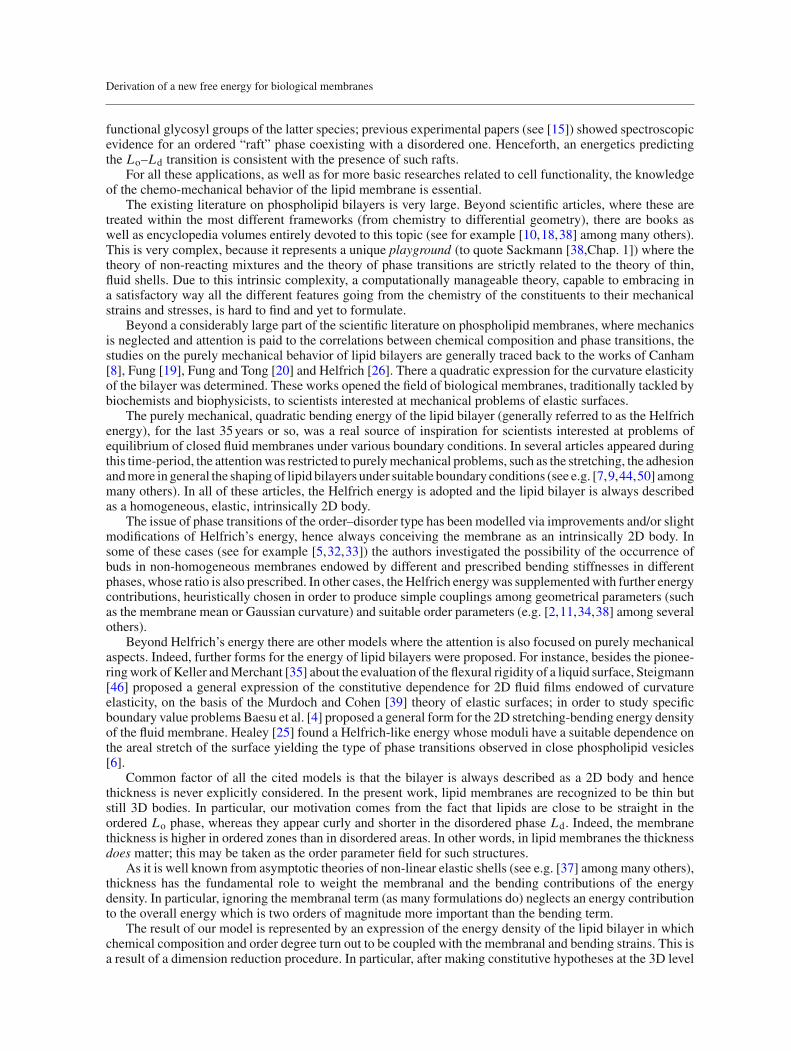
New and advanced high-resolution fluorescence imaging techniques (e.g. [6] in particular) have indeedhighlighted the coexistence of regions (or phases) characterized by different curvature, chemical compositionand degree of order of the phospholipid molecules (see Fig. 1). For the sake of argument the concept of orderis here referred to the single molecule, although in reality clusters of them are observed to be in the givenphase. Depending on the temperature of the environment and on the surrounding conditions, each phospholipidmolecule admits an ordered state, where the hydrophobic tails appear straightened and taller, and a disorderedstate, where the tails appear curly and shortened. Lipid membranes are also fluid-in-plane, which means thatmolecules are free to move on the membrane surface; for these reasons, the two phases are often referred toas liquid ordered (Lo) and liquid disordered (Ld) (e.g. [6,36]).

The above mentioned experimental results lead to think that there may exist a strong interplay amongmembrane shape, order and chemical composition during loading; this paper represents an attempt toward abetter comprehension of the correlation among these three aspects.

Liposomes do not merely capture attention because of their fascinating phase transitions; they representprototypical structures of cell membranes, basic bricks of each living organism. The chemo-mechanical beha-vior of the cell membrane is strictly related to the control of biological functions: for this reason, the studyof the phase-transition behavior of liposomes represents a step toward a better comprehension of the cellfunctionality. Furthermore, in recent years, liposomes have been widely adopted in the most advanced appli-cations of pharmaceutics (for example, the targeted delivery of drugs), of diagnostic, of bio-engineering (forinstance to build biosensors, where membranes are combined with optoelectronic devices), of food industry, ofcosmetics (see [38], Chap. 10 for an overview on these topics). Another interesting feature of cell membranesis, in some cases, the presence of lipid rafts (see [15] among many others); these are domains enriched of aparticular type of lipids, called glycosphingolipid. Such rafts may be induced in artificial biomembranes, suchas GUVs, and they have the key property that they are detergent-resistant. Lipid rafts basically occur when, forexample, fully saturated chains of sphingomyelin and glycosphingolipids bonding between neighboring active

Fig. 1 Images experimentally obtained by Baumgart et al. [6], showing how phase separation is strictly related to the equilibriumshapes of GUVs in water solution. In red and blue (in the online version) respectively, liquid-disordered and liquid-orderedphases. Scale bars 5µm (images by courtesy of Tobias Baumgart)


functional glycosyl groups of the latter species; previous experimental papers (see [15]) showed spectroscopicevidence for an ordered “raft” phase coexisting with a disordered one. Henceforth, an energetics predictingthe Lo–Ld transition is consistent with the presence of such rafts.

For all these applications, as well as for more basic researches related to cell functionality, the knowledgeof the chemo-mechanical behavior of the lipid membrane is essential.

The existing literature on phospholipid bilayers is very large. Beyond scientific articles, where these aretreated within the most different frameworks (from chemistry to differential geometry), there are books aswell as encyclopedia volumes entirely devoted to this topic (see for example [10,18,38] among many others).This is very complex, because it represents a unique playground (to quote Sackmann [38,Chap. 1]) where thetheory of non-reacting mixtures and the theory of phase transitions are strictly related to the theory of thin,fluid shells. Due to this intrinsic complexity, a computationally manageable theory, capable to embracing ina satisfactory way all the different features going from the chemistry of the constituents to their mechanicalstrains and stresses, is hard to find and yet to formulate.

Beyond a considerably large part of the scientific literature on phospholipid membranes, where mechanicsis neglected and attention is paid to the correlations between chemical composition and phase transitions, thestudies on the purely mechanical behavior of lipid bilayers are generally traced back to the works of Canham[8], Fung [19], Fung and Tong [20] and Helfrich [26]. There a quadratic expression for the curvature elasticityof the bilayer was determined. These works opened the field of biological membranes, traditionally tackled bybiochemists and biophysicists, to scientists interested at mechanical problems of elastic surfaces.

The purely mechanical, quadratic bending energy of the lipid bilayer (generally referred to as the Helfrichenergy), for the last 35 years or so, was a real source of inspiration for scientists interested at problems ofequilibrium of closed fluid membranes under various boundary conditions. In several articles appeared duringthis time-period, the attention was restricted to purely mechanical problems, such as the stretching, the adhesionand more in general the shaping of lipid bilayers under suitable boundary conditions (see e.g. [7,9,44,50] amongmany others). In all of these articles, the Helfrich energy is adopted and the lipid bilayer is always describedas a homogeneous, elastic, intrinsically 2D body.

The issue of phase transitions of the order–disorder type has been modelled via improvements and/or slightmodifications of Helfrich’s energy, hence always conceiving the membrane as an intrinsically 2D body. Insome of these cases (see for example [5,32,33]) the authors investigated the possibility of the occurrence ofbuds in non-homogeneous membranes endowed by different and prescribed bending stiffnesses in differentphases, whose ratio is also prescribed. In other cases, the Helfrich energy was supplemented with further energycontributions, heuristically chosen in order to produce simple couplings among geometrical parameters (suchas the membrane mean or Gaussian curvature) and suitable order parameters (e.g. [2,11,34,38] among severalothers).

Beyond Helfrich’s energy there are other models where the attention is also focused on purely mechanicalaspects. Indeed, further forms for the energy of lipid bilayers were proposed. For instance, besides the pionee-ring work of Keller and Merchant [35] about the evaluation of the flexural rigidity of a liquid surface, Steigmann[46] proposed a general expression of the constitutive dependence for 2D fluid films endowed of curvatureelasticity, on the basis of the Murdoch and Cohen [39] theory of elastic surfaces; in order to study specificboundary value problems Baesu et al. [4] proposed a general form for the 2D stretching-bending energy densityof the fluid membrane. Healey [25] found a Helfrich-like energy whose moduli have a suitable dependence onthe areal stretch of the surface yielding the type of phase transitions observed in close phospholipid vesicles[6].

Common factor of all the cited models is that the bilayer is always described as a 2D body and hencethickness is never explicitly considered. In the present work, lipid membranes are recognized to be thin butstill 3D bodies. In particular, our motivation comes from the fact that lipids are close to be straight in theordered Lo phase, whereas they appear curly and shorter in the disordered phase Ld. Indeed, the membranethickness is higher in ordered zones than in disordered areas. In other words, in lipid membranes the thicknessdoes matter; this may be taken as the order parameter field for such structures.

As it is well known from asymptotic theories of non-linear elastic shells (see e.g. [37] among many others),thickness has the fundamental role to weight the membranal and the bending contributions of the energydensity. In particular, ignoring the membranal term (as many formulations do) neglects an energy contributionto the overall energy which is two orders of magnitude more important than the bending term.

The result of our model is represented by an expression of the energy density of the lipid bilayer in whichchemical composition and order degree turn out to be coupled with the membranal and bending strains. This isa result of a dimension reduction procedure. In particular, after making constitutive hypotheses at the 3D level

L. Deseri et al.

(that include the enforcement of a new symmetry group introduced in [12]), we derive the Helmholtz energydensity per unit (reference mid-surface) area of the bilayer via asymptotic expansion of the bulk energy withrespect to a reference thickness. No heuristic coupling among the unknown fields is forced: the only recipesof the model are assumptions of constitutive and geometrical nature.

The resulting energy density confirms a precise hierarchy between local and non-local energy terms. Manyare the new and key results of the procedure worked out in the present paper:

– the local energy term is purely membranal and it appears completely determined on the basis of experimen-tally available information on the nature of the constituents;

– the non-local energy terms account for both bending effects and for a gradient term, penalizing the spatialvariations of a field related to the order–disorder transition;1

– strikingly, the gradient term spontaneously arises from the dimension reduction procedure, rather than beingheuristically introduced in the model;

– even more striking is the fact that the bending counterpart of the resulting energy is completely determined bythe knowledge of the local-purely membranal energy density; this implies that, in essence, such membranalcontribution is the only needed constitutive information of the model. Furthermore, such information canbe strictly related to the chemical composition of the membrane.

2 Assumptions of the model

On the grounds of the experimental evidences discussed in Sect. 1, we formulate the following assumptions:

(a) for GUVs, the small ratio between thickness and diameter (few nanometers vs. micrometers) fully justifiesthe assumption of thin shells;

(b) we ignore effects leading to a spontaneous or natural curvature of the bilayer and thus we assume that thenatural configuration of the membrane is flat;

(c) we assume that the membrane kinematics is restricted to the class of normal preserving deformations; thismeans that in our model lipid molecules remain orthogonal to the bilayer mid-surface; nevertheless, wedo not impose restrictions on the membrane thickness, which plays a crucial role in the Lo–Ld transition;

(d) we assume, according with assumption (b) of flat natural configuration, that the chemical compositionof the membrane is homogeneous moving along the bilayer mid-surface normal. A non-homogeneouschemical composition (as well as differences of pH or of electric charge) between the upper and lowermonolayers may induce a non-zero spontaneous curvature of the bilayer (e.g. [31]); such instance will betaken in consideration in a forthcoming generalization of the present model.

3 Dimension reduction procedure

3.1 Preliminary notions

The summation convention is assumed, unless otherwise specified. Greek indices take their values in the set{1, 2} and Latin indices take their values in the set {1, 2, 3}. Let (E1,E2,E3) be an orthonormal basis for theEuclidean point space R

3 and let a reference placement of a body B to occupy the open, bounded region B0of R

3. Let f be a smooth deformation of B0 into the current placement B = f (B0). Points of B0 will bedenoted by X = Xi Ei and their images in the current configuration B will be denoted by x = f (X).

Let S a smooth, open and oriented surface endowed at each point of a unit normal vector m, let TS := m⊥the tangent plane to S. The perpendicular projector of R

3 on TS is defined as

Pm := I − m ⊗ m

where I is the identity operator in the space Lin of linear transformations from R3 in R

3. Given a vectorfield c defined on B0, we denote the material gradient with respect to points X ∈ B0 by ∇c and the materialdivergence by Div c := tr(∇c) = ∇c ·I. Analogously, given a vector field b defined on B, we denote the spatialgradient with respect to points x ∈ B by grad b and the spatial divergence by div b := tr(grad b) = grad b · I.

1 The non-local energy reduces to the Helfrich’s one whenever the gradient term is negligible with respect to the bending oneand the elastic moduli do not significantly change with areal stretch and concentration.


Let now � and ω be smooth, open and oriented surfaces with unit normal m and n, respectively, bothsurfaces, respectively, endowed of non-zero intersections with B0 and B. The material and spatial surfacegradients of the vector fields c and b are defined by

∇�c := (∇c)Pm, gradωb := (grad b)Pn,

respectively. It is straightforward to check that

∇c = ∇c(Pm + m ⊗ m) = ∇�c + ∂c∂m

⊗ m,

grad b = grad b(Pn + n ⊗ n) = gradωb + ∂b∂n

⊗ n

where the normal derivatives of c and b are defined by

∂c∂m

:= (∇c)m,∂b∂n

:= (grad b)n.

Using a smooth extension of the unit normal field n to a neighborhood of ω, we can introduce the curvaturetensor of the surface as

L := −gradωn = −(grad n)Pn.

It can be proved (e.g. [23]) that the curvature tensor L is symmetric and it satisfies

Ln = 0.

The mean curvature and the Gaussian curvature of the surface ω are, respectively, defined by

H := 1

2trL, K := det L.

According to the Cayley–Hamilton theorem for symmetric rank-2 tensors, the curvature tensor L satisfies thefollowing useful identity

L2 − (trL)L + (det L)Pn = 0 �⇒ L2 − 2HL + K Pn = 0.

For tangential tensors, i.e. the ones for which at every point there exists a vector m such that A ≡ PmAPm, wemay use the following identification for their determinants: det A ≡ det[Aαβ ].

3.2 Geometry, chemistry and energetics in the bulk

Accordingly with assumption (b) of our model, we describe the natural configuration of the membrane as the3D cylindrical domain in R

3 defined as follows

B0 := {X = (X, X3) ∈ �× (−h0/2, h0/2)} (1)

being� an open, bounded and simply connected region in R2 and h0 the constant membrane thickness. Points

of the membrane mid-surface� have been denoted by X = XαEα . Let f be a smooth deformation of the bodyfrom its reference configuration B0 to its current configuration B := f (B0) ⊂ R

3 and let the 3D deformationgradient be F := ∇f . We will assume that the body is made of a non-reacting mixture of C constituentmolecules, differing from each other for the chemical structure and composition. At each point of the currentconfiguration of the body B it is possible to define the molar fractions

χ3Dk (x) := dNk(x)

dNtot(x), k = 1, . . . ,C

where dNk(x) and dNtot(x) = ∑Ck=1 dNk(x) represent a measure of the number of molecules of the k-th

constituent and a measure of the total number of molecules contained in a neighbor of the point x = f (X) (inthe current configuration), respectively. The material description of the molar concentration fields reads as

χ3Dk := χ3D

k ◦ f .

L. Deseri et al.

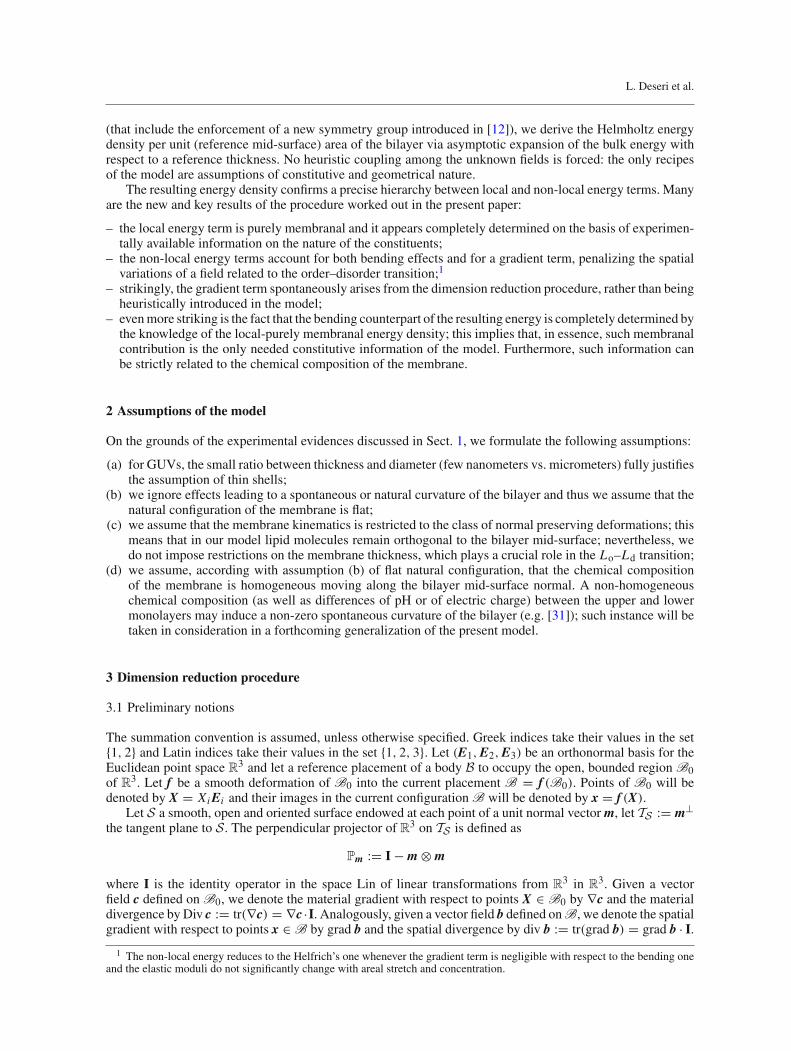
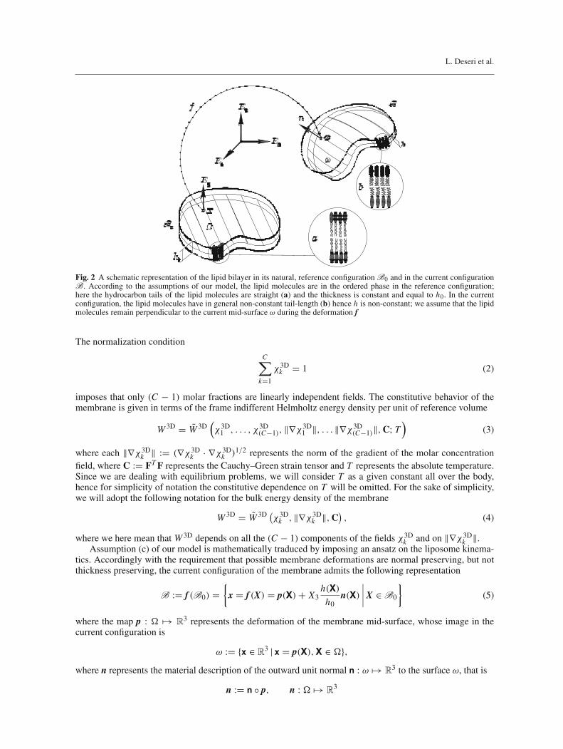
Fig. 2 A schematic representation of the lipid bilayer in its natural, reference configuration B0 and in the current configurationB. According to the assumptions of our model, the lipid molecules are in the ordered phase in the reference configuration;here the hydrocarbon tails of the lipid molecules are straight (a) and the thickness is constant and equal to h0. In the currentconfiguration, the lipid molecules have in general non-constant tail-length (b) hence h is non-constant; we assume that the lipidmolecules remain perpendicular to the current mid-surface ω during the deformation f

The normalization condition

C∑

k=1

χ3Dk = 1 (2)

imposes that only (C − 1) molar fractions are linearly independent fields. The constitutive behavior of themembrane is given in terms of the frame indifferent Helmholtz energy density per unit of reference volume

W 3D = W 3D(χ3D

1 , . . . , χ3D(C−1), ‖∇χ3D

1 ‖, . . . ‖∇χ3D(C−1)‖,C; T

)(3)

where each ‖∇χ3Dk ‖ := (∇χ3D

k · ∇χ3Dk )1/2 represents the norm of the gradient of the molar concentration

field, where C := FT F represents the Cauchy–Green strain tensor and T represents the absolute temperature.Since we are dealing with equilibrium problems, we will consider T as a given constant all over the body,hence for simplicity of notation the constitutive dependence on T will be omitted. For the sake of simplicity,we will adopt the following notation for the bulk energy density of the membrane

W 3D = W 3D (χ3D

k , ‖∇χ3Dk ‖,C

), (4)

where we here mean that W 3D depends on all the (C − 1) components of the fields χ3Dk and on ‖∇χ3D

k ‖.Assumption (c) of our model is mathematically traduced by imposing an ansatz on the liposome kinema-

tics. Accordingly with the requirement that possible membrane deformations are normal preserving, but notthickness preserving, the current configuration of the membrane admits the following representation

B := f (B0) ={

x = f (X) = p(X)+ X3h(X)h0

n(X)∣∣∣∣ X ∈ B0

}

(5)

where the map p : � �→ R3 represents the deformation of the membrane mid-surface, whose image in the

current configuration is

ω := {x ∈ R3 | x = p(X),X ∈ �},

where n represents the material description of the outward unit normal n : ω �→ R3 to the surface ω, that is

n := n ◦ p, n : � �→ R3


and where h(X) represents the material description of the thickness of the current configuration h(x), that ish = h ◦ p.2

From now on, any dependence on the coordinates (X, X3)will be stressed just when necessary; in particular,we recall that the scalar and vector fields h, p and n do not depend on X3. For the sake of simplicity, let us set

φ := h/h0,

so that the 3D gradient of the deformation, which now may be written in terms of φ since f = p + X3φ n,reads as follows

F = ∇f = ∇p + φn ⊗ E3 + X3 [n ⊗ ∇φ + φ∇n] .

On setting for simplicity P3 = PE3 and recalling that I = P3 +E3 ⊗E3, the gradient F can be recast as follows

F = F(P3 + E3 ⊗ E3) = ∇�p + φE3 + X3[n ⊗ ∇�φ − φL(∇�p)

]

= F + φn ⊗ E3 + X3[n ⊗ ∇�φ − φLF

](6)

where F := ∇�p represents the surface gradient of deformation of fibers lying on the reference mid-surface� and where L is the material description of the curvature tensor L of the current mid-surface ω, namely

L := L ◦ p, L := −(grad n)Pn = −gradωn.

We remark that since

FE3 = 0, FT n = 0, L = LT , Ln = 0,

the following useful identities hold

F ≡ PnFP3, L ≡ PnLPn.

The right Cauchy–Green tensor C = FT F arising from the explicit expression of the deformation gradient (6)can be put in the form

C(X, X3) = C0(X)+ X3C1(X)+ X23C2(X) (7)

where the three symmetric tensors C j (X) ( j = 1, 2, 3) are

C0 := FT F + φ2E3 ⊗ E3 = G + φ2E3 ⊗ E3;C1 := −2φFT LF + φ(∇�φ ⊗ E3 + E3 ⊗ ∇�φ);C2 := ∇�φ ⊗ ∇�φ + φ2FT L2F,

where the tensor

G := FT F

evidently represents the Cauchy–Green tensor of the mid-surface �. For later use, let us also calculate theCauchy–Green tensor relative to fibers laying on planes parallel to the reference mid-surface �, namely thetensor

C(X, X3) := [F(X, X3)P3]T [F(X, X3)P3] = P3C(X, X3)P3

which can be expanded as follows

C(X, X3) = C0(X)+ X3C1(X)+ X23C2(X) (8)

2 For simplicity of notation we will set for any arbitrary scalar, vector of tensor function ξ

ξ(X, 0) := ξ(X).

L. Deseri et al.

where the three symmetric tensors C j (X) ( j = 1, 2, 3) are

C0 := FT F = G;C1 := −2φFT LF;C2 := ∇�φ ⊗ ∇�φ + φ2FT L2F.

Furthermore it may be easily checked that

C33 = CE3 · E3 = φ2. (9)

3.3 In-plane-fluidity in the bulk

As already mentioned in Sect. 1, within this model we focus attention on the so-called liquid phases Lo andLd; in such phases the membrane behaves like an in-plane-fluid, which roughly means that lipid moleculescan move freely on the membrane surface. From the mechanical point of view, in-plane-fluidity means thatthe membrane does not offer resistance to shears contained in planes orthogonal to E3. The derivation of asuitable symmetry group which describes the peculiarity of in-plane-fluidity at the level of the bulk materialwas obtained in [12], where an expression of the reduced bulk energy density starting from a frame invariantbulk energy density was given. According to [12], this material property can be imposed by requiring invarianceof the constitutive response under the group of transverse unimodular transformations with axis E3, namelythe set

Unim{E3} := {H = HαβEα ⊗ Eβ + E3 ⊗ E3 with det H = 1},that is deformations which leave unaltered the area of planes parallel to the reference mid-surface�. Invarianceof the energy density (4) under the symmetry transformations group is imposed by requiring that

W 3D(·, ·, (FH)T (FH)) = W 3D(·, ·,FT F), ∀H ∈ Unim{E3},where bullets represent scalars which are unaffected by the symmetry transformation. As it is shown in [12],invariance under the group of transverse unimodular transformations implies the following reduced form ofthe bulk energy density (4):

W 3D = ˜W 3D (χ3D

k , ‖∇χ3Dk ‖, det C, det C,C33

)(10)

where C is the rank-2 tensor defined by

C := P3CP3 = CαβEα ⊗ Eβ.

For the sake of simplicity in the forthcoming calculations, we set

δ := det C, := det C. (11)

3.4 Asymptotic expansion of the stored energy

The Helmholtz energy stored in the body can be calculated by integration of the bulk energy density over thereference configuration B0

E :=∫

B0

W 3D(X, X3) dA dX3, (12)

being dA the area measure on the reference mid-surface �. We now make the following change of variablesfrom B0 to a rescaled domain B1 which is independent of h0 via the re-parametrization

r : Z = (Z, Z3) ∈ B1 −→ X = (X, X3) = (Z, h0 Z3) ∈ B0.


The rescaled domain B1 is defined by

B1 :={

Z = (Z, Z3) ∈ �×(

−1

2,

1

2

)}

(13)

and since the Jacobian of the re-parametrization r equals h0, then dV0 = dAdX3 = dAh0dZ3 = h0dV1. Afterthe change of variables the integral (12) takes the form

E =∫

B1

h0W 3D(Z, h0 Z3) dA dZ3.

On the grounds of the assumption (a) of small bilayer membrane thickness, it makes sense to consider anasymptotic expansion of E with respect to the constant reference thickness h0 (the dependence on h0 is herestressed on purpose)

E(h0) = [E(h0)]h0=0 + h0

[d(h0)

dh0

]

h0=0+ h2

0

2

[d2 E(h0)

dh20

]

h0=0

+ o(h20). (14)

In the purely mechanical context, an analog procedure was performed in [27–29] and more recently in [47].Within our model we will neglect terms of order higher than the second and we will show that the consideredones account for local membranal effects, for non-local membranal effects related to the order/disorder phasetransition and for bending effects. Since B1 is independent of h0, we can carry on the asymptotic expansionof E in powers of h0 by expanding its integrand around h0 = 0; this yields

E =∫

B1

h0

{

[W 3D]h0=0 + h0

[dW 3D

dh0

]

h0=0+ h2

0

2

[d2W 3D

dh20

]

h0=0

}

dA dZ3. (15)

In order to derive the expression of the surface energy density of a thin lipid bilayer which satisfies theassumptions (a)–(d) of our model, we will now consider the special form of the bulk energy (4) for lipidbilayers endowed of in-plane-fluidity, with the expressions of the tensors C and C given by Eqs. (7) and (8).

As first thing, in agreement with the assumption (d) of our model, we impose invariance of the molarfraction fields χ3D

k with respect to the coordinate X3 by setting

χ3Dk (X, X3) ≡ χ3D

k (X, 0) =: χk(X) ∀X ∈ B0.

By the expressions (7)–(9) we also know that the determinants = det C and δ = det C depend on h0, whileC33 = φ2 thus it does not depend on h0. On stressing the dependence on h0, it thus makes sense to set forsimplicity

w = w(δ(h0),(h0)) := ˜W 3D(χk, ‖∇χk‖, δ(h0),(h0),C33). (16)

The asymptotic expansion of w with respect to h0 yields

w(δ(h0),(h0)) = w(δ(0),(0))+ h0 ˙w(δ(0),(0))+ h20

2¨w(δ(0),(0))+ o(h2

0), (17)

where derivation with respect to h0 has been denoted by the dot. We record the following relations:

w = wδδ + w

w = wδδ + w+ wδδδ2 + w

2 + 2wδδ.

Detailed calculations of the derivatives of δ andwith respect to h0 are worked out in Appendix; the resultingexpressions, calculated at h0 = 0 are

(0) = φ2 J 2

(0) = −4Z3φ3 J H

(0) = 4Z23 J 2φ4 K + 8Z2

3φ4 H2

L. Deseri et al.

δ(0) = J 2

δ(0) = −4Z3 J 2φH

δ(0) = Z23

(8φ2 J 2 H2 + 4φ2 J 2 K + 2J 2‖gradωφ‖2

m

);

here

J = (det G)1/2

represents the areal stretch measured at a place of the reference mid-surface�, where H and K are, respectively,the material descriptions of the mean and Gaussian curvatures in a (corresponding) place of the current mid-surface ω.3

The asymptotic expansion of the energy (17) yields an explicit dependence on the coordinate Z3, hence itis now possible to obtain the surface energy density of the membrane by integration over the thickness of therescaled domain B1; linear terms in Z3, which factor w, cancel during integration, and after straightforwardcalculations we finally get that the stored Helmholtz energy can be expressed as

E =∫

�

ϕ(χk,∇χk, J, φ, H, K , ‖gradφ‖m) dA

where ϕ represents the surface Helmholtz energy, per unit reference area, given by

ϕ = ϕloc + h20ϕ

nloc. (18)

The local energy density ϕloc is defined by

ϕloc := ϕloc(χk,∇χk, J, φ) := h0

[ ˜W 3D(χk,∇χk, δ,,C33)]

δ=J 2,=φ2 J 2,C33=φ2(19)

and where the non-local energy density ϕnloc is defined by

ϕnloc := ϕnloc(χk,∇χk, J, φ, H, K , ‖gradωφ‖2

m

):= κ1 H2 + κ2 K + β‖gradωφ‖2

m (20)

with the bending moduli κ1,2 and the non-local modulus β completely determined in terms of the bulk energyW 3D by the relations

κ1 = κ1(χk,∇χk, J, φ) := (φ2 J 2w1 + φ4w2 + 2J 4φ2w3 + 2φ6 J 2w4 + 4J 3φ4w5

)/3,

κ2 = κ2(χk,∇χk, J, φ) := (φ2 J 2w1 + J 2φ4w2

)/6 (21)

β = β(χk,∇χk, J, φ) := w1 J 2/12,

and where, conclusively, we have set

w1 := h0

[ ˜W 3Dδ (χk,∇χk, δ,,C33)

]

δ=J 2,=φ2 J 2,C33=φ2,

w2 := h0

[ ˜W 3D (χk,∇χk, δ,,C33)

]

δ=J 2,=φ2 J 2,C33=φ2,

w3 := h0

[ ˜W 3Dδδ (χk,∇χk, δ,,C33)

]

δ=J 2,=φ2 J 2,C33=φ2, (22)

w4 := h0

[ ˜W 3D(χk,∇χk, δ,,C33)

]

δ=J 2,=φ2 J 2,C33=φ2,

w5 := h0

[ ˜W 3Dδ (χk,∇χk, δ,,C33)

]

δ=J 2,=φ2 J 2,C33=φ2.

The expression of the surface energy density ϕ, consistently derived from the bulk energy (10), represents themain target of our model. Its structure establishes a precise hierarchy between local terms, which factor h0,and non-local terms, which factor h3

0. Worth noting, the bending/non-local moduli constitutively depend onlocal fields, which express the chemical composition, the areal stretch at the level of the bilayer mid-surfaceand the bilayer thickness variations.

3 Here φ is the spatial description of φ, in the sense that φ = φ ◦ p. The term ‖.‖2m represents the material description of ‖.‖2.


3.5 Quasi-incompressibility

The expressions of the moduli given in general form in Eqs. (21), (22) can be appreciably simplified on thebasis of a further assumption on the bulk behavior of the bilayer.

Indeed, besides their full generality, Eqs. (21), (22) may result of no practical use. Nevertheless, there arestrong experimental evidences that lipid molecules behave keeping their volume constant; this in turn impliesthat the mid-surface areal stretch J and the thickness extension (or contraction) φ in a thin biomembrane arenot independent fields. In order to provide an experimental justification of these further assumptions on thebilayer behavior, let us review some well known discussions on the topic from the biophysical literature onbiomembranes.

According to the encyclopedia article on biological membranes by Lipowsky and Sackmann [38], “. . .thehydrocarbon film within the membrane is essentially incompressible, stretching of the bilayer area implies athinning of the bilayer thickness. . .”.

According to Safran [45], the assumption of quasi-incompressibility is proper since “. . .in addition tobeing characterized by the area per amphiphile, the . . . membrane is also characterized by its thickness [h],which can also change under deformations of the film . . . we assume that the equation of state of the flatmembrane determines the thickness as a function of the area per molecule. (A simple example is the case ofan incompressible molecule where the product of [Jφ] is constrained to equal the molecular volume so that[Jφ = 1]). We thus take the flat membrane to be characterized only by the area per molecule. . . ”, where insquare brackets we adopt our notation for the same entities used by the Authors.

About molecular volume incompressibility, Goldstein and Leibler [21], “. . .adopt the viewpoint that theselyotropic liquid crystals may be treated in analogy with conventional models of binary liquid mixtures, namelythat the two components of the system, lipid and water, are assumed to be characterized by invariant molecularvolumes vl and vw. . . the bilayer thickness [h] and effective area per head group are simply related byh = vl”.

For these reasons we impose that in thin biomembranes the fields J and φ are related at each point by therelation

Jφ = 1. (23)

It is easy to check that the relation (23) can be seen as an quasi-incompressiblity constraint for a thin membrane;indeed, according to the constrained kinematics deriving from the ansatz (5), the volume variation det F = √

is given by

det F = φ J − 2X3φ2 H + X2

3 Jφ3 K ;under the constraint (23) the volume variation at each point of the membrane becomes

det F = 1 − 2X3φ2 H + X2

3φ2 K

which shows that the exact incompressibility constraint is actually satisfied for points X = (X, 0) belongingto the bilayer mid-surface, whereas it is not satisfied in general for points with X3 �= 0. In general, it resultsthat

det F = 1 + O(h0),

and for this reason, in the limit of thin bilayers where h0 → 0, we define the requirement (23) as a quasi-incompressibility constraint.

It should be remarked that relation (23) also plays a crucial role in the definition of a suitable coarse-grained order parameter for the order–disorder phase transition in the biomembrane: such transition is indeeddetectable both by the straightening/shortening of the hydrocarbon tails, and by the variation of the head-grouparea, roughly speaking the measure of the transversal cross section of a single lipid molecule.

In light of the discussion above, we restrict our attention to bulk energy densities of the form

W 3D = ˜W 3D (

χ3Dk , ‖∇χ3D

k ‖, δ) , (24)

with δ defined by (11). Obviously, this type of energy is a special case of (10).This energy may capture the main features of a thin biomembrane undergoing the Lo–Ld order–disorder

phase transition; indeed, for a thin body, it results that ≈ 1 and that C33 is deducible by δ evaluated at any

L. Deseri et al.

arbitrary point of the mid-surface; the latter is indeed the areal stretch J measured at any point right on sucha surface.

It should be remarked that in Eq. (24), δ(X) actually depends on all the coordinates (X, X3). For this reason,the expression of the energy density (24) leads to think about this model as a thin, continuous layer of fluidelastic surfaces, whose energy density (beyond chemical composition) solely feels local variations of area onplanes perpendicular to E3 and whose kinematics is restricted by the ansatz (5).

It is now straightforward to check that the expressions of the moduli (21) and (22) undergo a strongsimplification, since in this special case it results that

w2 = w4 = w5 = 0,

hence the bending and non-local moduli are completely determined as functions of derivatives of the bulkenergy with respect to δ. In particular, letting J the spatial description of J , that is J = J ◦ p, it results that

φ J = 1 �⇒ gradωφ = − J−2gradω J �⇒ ‖gradωφ‖2m = J−4‖gradω J‖2

m

hence we get that the Helmholtz energy density per reference area unit admits the following simplified expres-sions for the local counterpart of the energy density

ϕloc := ϕloc(χk,∇χk, J ) := h0

[ ˜W 3D(χk,∇χk, δ)

]

δ=J 2(25)

and for the non-local counterpart of the energy density

ϕnloc := ϕnloc(χk,∇χk, J, H, K , ‖gradω J‖2

m

):= κ1 H2 + κ2 K + α‖gradω J‖2

m (26)

where again

κ1 = κ1(χk,∇χk, J ) := (w1 + 2J 2w3)/3,

κ2 = κ2(χk,∇χk, J ) := w1/6, (27)

α = α(χk,∇χk, J ) := w1/(12J 2),

with

w1 := h0

[ ˜W 3Dδ (χk,∇χk, δ)

]

δ=J 2,

w3 := h0

[ ˜W 3Dδδ (χk,∇χk, δ)

]

δ=J 2.

The final expression of the moduli may be evaluated after substituting ϕloc in place of W 3D, which gives

κ1 = κ1(χk,∇χk, J ) := 1

6

∂2ϕloc(χk,∇χk, J )

∂ J 2 ,

κ2 = κ2(χk,∇χk, J ) := 1

12J

∂ϕloc(χk,∇χk, J )

∂ J, (28)

α = α(χk,∇χk, J ) := 1

24J 3

∂ϕloc(χk,∇χk, J )

∂ J.

The final expression of the surface Helmholtz energy density per reference unit area for a quasi-incompressiblelipid bilayer is represented by

ϕ = ϕloc + h20

[1

6

∂2ϕloc

∂ J 2 H2 + 1

12J

∂ϕloc

∂ JK + 1

24J 3

∂ϕloc

∂ J‖gradω J‖2

m

]

(29)

This expression of the surface Helmholtz energy of the lipid membrane presents several novel featureswith respect to the existing literature on the argument, in particular:


(i) local and non-local effects are weighted by different powers of the bilayer reference thickness h0, inparticular local effects are two orders of magnitude more “important” than non-local ones; this shouldaddress attention to the fact that ignoring membranal effects may be inappropriate when studying theequilibrium of liposomes, although this is customarily done in all articles where the only Helfrich energydensity [26]

w = κ1 H2 + κ2 K (30)

with κα given constants is considered; as matter of fact, it would be easy to check that the Helfich energycan be simply recovered by ignoring chemical and membranal effects;

(ii) the gradient term which penalizes spatial variations of the thickness (that is, in our model, of the mid-surface areal stretch) and the relative modulus α are not heuristically introduced, rather these are consis-tently derived from the procedure of dimension reduction on the grounds of the assumptions of our model;this provides a tool in order to relate the amplitude of the boundary layer between the ordered–disorderedphases and the surface tension;

(iii) the fact that the interplay between K and (J−2‖gradω J‖2m) is penalized in Eq. (29) may not be surprising;

in other words, such energy penalizes local changes in the gradient of the areal stretch J (the determinantof the metric tensor, which is associated to the first fundamental form of the surface) and changes inGaussian curvature; as it is well known, Gauss Egregium theorem assures that the Gaussian curvature Kchanges only if the first fundamental form does; further, Brioschi’s formula gives the explicit expressionof K in terms of the first fundamental form. No other proposed energetics for biomembranes include theterm (K + J−2‖gradω J‖2

m/2), which is in general non-zero;(iv) the bending moduli κ1 and κ2 are not heuristically set equal to different constants for each phase domain

(what is customarily done in the literature on this topic, as discussed in Sect. 1), rather these moduliare known functions of the local energy term, which in turn is completely determined on the basis ofexperimental data on the mixture constituents.

4 Special forms of the energy density

Let us consider the special case of quasi-incompressible membranes whose energy density is given by Eq. (29).The dimension reduction procedure carried out in the previous section has shown that, within our model, thenon-local moduli κ1, κ2 and α can be calculated from Eq. (28) as functions of the local energy density ϕloc. Inessence, by Eq. (29), this energy represents the only needed constitutive information of our approach.

Researchers involved in laboratory analysis of GUVs’ properties generally make use of binary mixturesof ternary liposomes (e.g. [6,51–53]). For this reason in this work we confine attention to the to two cases ofbinary saturated lipid/unsaturated lipid and lipid/cholesterol mixtures. This choice does not obviously representa limit for our theory, which is fully general and virtually applies to more complex cases.

In establishing the expression of the surface Helmholtz energy ϕloc of both kinds of mixtures, we hereconsider the membrane as a surface made of a compound of two non-reacting components. Because of thenormalization condition (2), there is one only independent molar fraction field χ .

Within this intrinsically 2D approach, the order–disorder phase transition is entrusted with the mid-surfaceareal stretch J , univocally related to the bilayer current thickness h by the relation h J = h0. Accordingly, wearbitrarily assume that the reference configuration of the surface is in the ordered phase Lo, which correspondsto J = 1 (that is h = h0).

The existing literature on non-reacting mixtures offers nowadays a huge variety of phenomenologicalmodels providing suitable expressions for the Helmholtz energy ϕloc in different cases. Most of these formulasare based on a bottom-up approach: this allows for finding the (effective) local part of the free energy densitystarting from mean field approaches employed in statistical mechanics (see e.g. [42,Chap. 3], and referencescited therein); this part of the energy accounts for short-to-medium range interactions among lipids and/orcholesterol.

A family of energies for ϕloc may be considered, in which the temperature of the environment T may beassumed as the parameter for such family. This may be provided by the models cited above, among whichwe recognize a common structure for the energy density of liquid, binary mixtures undergoing order–disorderphase transitions. This is essentially represented by the following form

ϕloc(χ, ‖∇χ‖, J ; T ) = [ϕloc

chem(χ; T )+ γ (χ)‖∇χ‖2] + ϕlocelast(χ, J ; T ), (31)

L. Deseri et al.

where the term ϕlocchem represents the classical enthalpic/entropic energy density for mixtures, ϕloc

elast representsthe membranal elastic energy density and the term γ ‖∇χ‖2 represents the free energy cost due to concentrationgradients.

Without entering the details of the derivation, for the particular cases of saturated lipid/unsaturated lipidmixtures (��) and lipid/cholesterol mixtures (�c), accordingly to the work by Komura et al. [36], we take theexpressions for the local counterparts of the local energy density derived in (31) and listed in the sequel:

(��) mixtures: here, the purely chemical counterpart of the energy density (31) has the form

ϕlocchem = ρ0

[ψ0 + ψ id

mix + ψe].

Here ρ0 represents the molar density per unit of area of the reference configuration, while

ψ0 = µ01χ + µ0

2(1 − χ)

represents the formation energy, being µ0i the standard chemical potentials of each component and

ψ idmix = RT [χ ln χ + (1 − χ) ln(1 − χ)]

represents the classical ideal energy of mixing, with R a material constant. The so-called excess energyψe

represents a correction to the ideal energy of mixing deriving from different interactions between like andunlike particles in the aggregate. A typical form of such contribution is represented by the Bragg–Williamsenergy (see e.g. [42, Sect. 3.3] and references cited therein), i.e.:

ψe = wχ(1 − χ)

where w represents the interaction parameter.4 For the elastic counterpart of the energy density, a Landauexpansion with respect to the order parameter J is assumed by slightly adapting the expression proposedin [36]. In particular, we take the following expression for such free energy:

ϕlocelast = a2

2[T ∗(χ)− T ](J − 1)2 + a3

3(J − 1)3 + a4

4(J − 1)4

where the constants a2 > 0, a3 < 0, a4 > 0 are experimentally determined (see [36]) and where T ∗(χ)represents a reference temperature for the order–disorder transition, depending on the pointwise valueof the chemical concentration. In agreement with [36], we adopt for T ∗(χ) a simple linear interpolationbetween the reference temperatures of both constituents of the mixture, that is

T ∗(χ) = χT ∗s + (1 − χ)T ∗

u

where T ∗s and T ∗

u , respectively, represent reference temperatures related to the Lo–Ld transition in pure satu-rated and pure unsaturated mixtures, respectively. The proposed expression of ϕloc

elast presents a temperature-modulated non-convexity in J ; this is essential in order to capture the Lo–Ld transition;

(�c) mixtures: here, the purely chemical counterpart of the energy density has the form

ϕlocchem = ρ0

[ψ0 + ψFH

mix + ψe] .

where the term ψ0 has the same expression given for (��) mixtures; the mixing energy is derived on thebasis of the Flory–Huggins polymer solution theory (see e.g. [42, Sect. 3.5], and references cited therein)and it has the form

ψFHmix = RT [χc ln 2χc + (1 − 2χc) ln(1 − 2χc)]

where χc represents the mole fraction of cholesterol in the mixture. We refer the interested readers to thearticle [36] and to the book by Hill [30] for further details on the Flory–Huggins theory and its applicationsin lipid–cholesterol mixtures. The excess contribution ψe here accounts for the different roles played bycholesterol in (�c) mixtures toward the order–disorder phase transition; Komura et al. [36], in order to

4 In classical models w is understood not to depend upon the measure of the local stretch, although it should. Nevertheless, asa first approximation, here we assume w as a constant.


phenomenologically describe the experimental evidence that at small concentrations cholesterol favorsthe disordered Ld phase, while at higher concentrations it favors the ordered Lo phase, introduced thefollowing term

ψe = 1

J(�1χc − �2χ

2c ),

where �i are experimentally determinable constants. The elastic counterpart of the energy has here thesame form already discussed for (��) mixtures, but here T ∗ is simply the reference temperature of the purelipid system.

This completes the determination of the local energy density for the two considered cases of binary modelmembranes. In both cases of (��) and (�c) mixtures, the concentration dependent penalization moduli γis a constant depending on the mixture constituents and interactions (see for example [45] for more detailedexpositions on the argument). Once the local energy term has been determined, Eq. (28) permits the calculationof the bending and non-local moduli κ1,2 and α; at this point the construction of the energetics (29) of thebiological membrane is finally complete.

Let us now calculate for example the expression of the bending and non-local moduli in the case of (��)mixtures. After straightforward calculations, we get that

κ(��)1 = a2

6[T ∗(χ)− T ] + a3

3(J − 1)+ a4

2(J − 1)2,

κ(��)2 = a2(J − 1)

12J[T ∗(χ)− T ] + a3(J − 1)2

12J+ a4(J − 1)3

12J, (32)

α(��) = a2(J − 1)

24J 3 [T ∗(χ)− T ] + a3(J − 1)2

24J 3 + a4(J − 1)3

24J 3 .

It is worth noting that our procedure naturally yields coupling among the independent fields χ, J, H and Kwhich substantially agree with some heuristic models proposed in the biophysical literature on phase transitionsin lipid bilayers.

Indeed, expanding the energy (29) with moduli given by Eq. (32), we see that for the particular case oflipid–lipid mixtures, the following coupling among χ, J, H and K arises:

ϕcoupl(χ, J, H, K ) = c0χH2 + g0(J )H2 + g1(J )χK + g2(J )K (33)

where c0 is a constant and gi (J ) (i = 0, 1, 2) are known polynomials of J . In particular, Ayton et al. [2] adoptin their expression of the energy a coupling term between chemical composition and mean curvature of theform

wAyton(χ, H) ≈ χH2,

which is recovered from (33) by setting gi = 0. Chen et al. [11] adopt a coupling term among the chemicalcomposition and the Gaussian curvature of the form

wChen(χ, K ) ≈ χK ,

which is recovered from (33) by setting c0 = g0 = g2 = 0 and tacitly ignoring the dependence on J . In theprevious models, no dependence upon T is accounted for.

Returning to the discussion on our model, the expressions of the bending moduli derived in (32) for lipid–lipid mixtures offer the possibility of understanding how, even in the special case of null membranal tractions(i.e. ∂ϕloc/∂ J = 0), the order–disorder transition may have influence on the bending stiffness, in particular onκ1 (since as we have seen, in this case κ2 = α = 0). Indeed, it is possible to show [14] that for temperatures

T < T ∗ − 2a23

9a2a4

the energy density ϕloc reaches its absolute minimum at J = 1, that is in the ordered phase Lo, where themean curvature modulus attains the value

κ��1 (Lo) = a2

6[T ∗(χ)− T ].

L. Deseri et al.

Furthermore, for values of the external temperature

T > T ∗ − 2a23

9a2a4

the absolute minimum is attained at a value of the areal stretch Jd > 1, that is in the disordered phase Ld,where

κ��1 (Ld) =(a2

3 − 4a4a2τ)− a3

√a2

3 − 4a4a2τ

12a4;

for the sake of brevity we have set τ = T ∗ − T . If the externally controlled temperature equals the transitiontemperature

Ttr = T ∗ − 2a23

9a2a4

then a coexistence of two phases endowed of different bending moduli is expected.Naively, by picturing an isometric bending of an initially flat square membrane under opposite couples

applied along two opposite edges, the non-homogeneity of the bending modulus κ1 will naturally determinethe occurrence of phase domains with sensibly different curvatures.

We expect that this kind of behavior can explain the phase separation phenomena in GUVs, where thingsare indeed more complex because these are curved, closed surfaces, subject to internal pressure. In [14], wewill discuss in greater detail the applications of the energetics derived in the present paper and its generalizationto the case of non-negligible spontaneous curvature.

As a concluding remark, it is worth noting that since we assumed that the natural configuration of themembrane is flat, we expect that the derived expression of the energy (29) attains a minimum at J = 1, H = 0and K = 0. As matter of fact, the moduli evaluated at J = 1 read

κ(��)1 = a2

6[T ∗(χ)− T ], κ

(��)2 = α(��) = 0

where since the reference configuration is here assumed in the ordered phase Lo (J = 1) then T ∗ − T > 0 andthus κ1 > 0. The energy density (29) evaluated at J = 1 becomes

ϕ = a2

6[T ∗(χ)− T ]H2

which indeed has a minimum at H = 0, hence the flat configuration with H = K = 0 is in particular anabsolute minimizer for the surface energy; nevertheless, the fact that variations of K do not appear in theexpression of ϕ evaluated at J = 1 means that as long as the membrane is not kept in a regime of membranaltension (that is, as long as ∂ϕloc/∂ J = 0) then all configurations endowed of constant, zero mean curvatureare natural configurations for the membrane, i.e. absolute minimizers of the surface energy density (29).

Acknowledgments Special thanks go to Timothy J. Healey, for stimulating the interest in this topic and for the endless conver-sation on the topic in the last few years and to Roberto Paroni, for continuous and extremely useful conversations through the lastyears about the topic of thin structures and in particular on dimension reduction procedures and differential geometry. The authorswish to thank Tobias Baumgart, Sovan Das and James T. Jenkins for the very useful conversations on the subject and relatedissues through the last few years. G. Zurlo gratefully acknowledges the Department of Theoretical and Applied Mechanics atCornell University and the Center for Non-linear Analysis, Department of Mathematical Sciences at Carnegie-Mellon Universityfor hospitality and support during his extended visits. M. D. Piccioni and G. Zurlo acknowledge Professor Salvatore Marzano forhis advice and support and the D.I.C.A. Politecnico di Bari for the financial support.

Appendix

In this section, we work out the main calculations needed in the article. As first thing let us calculate theexpression of the det F with F deriving from the ansatz (5). As we have seen the current mid-surface of thebilayer is defined as

ω := {x = p(X), X ∈ � ⊂ R2}.


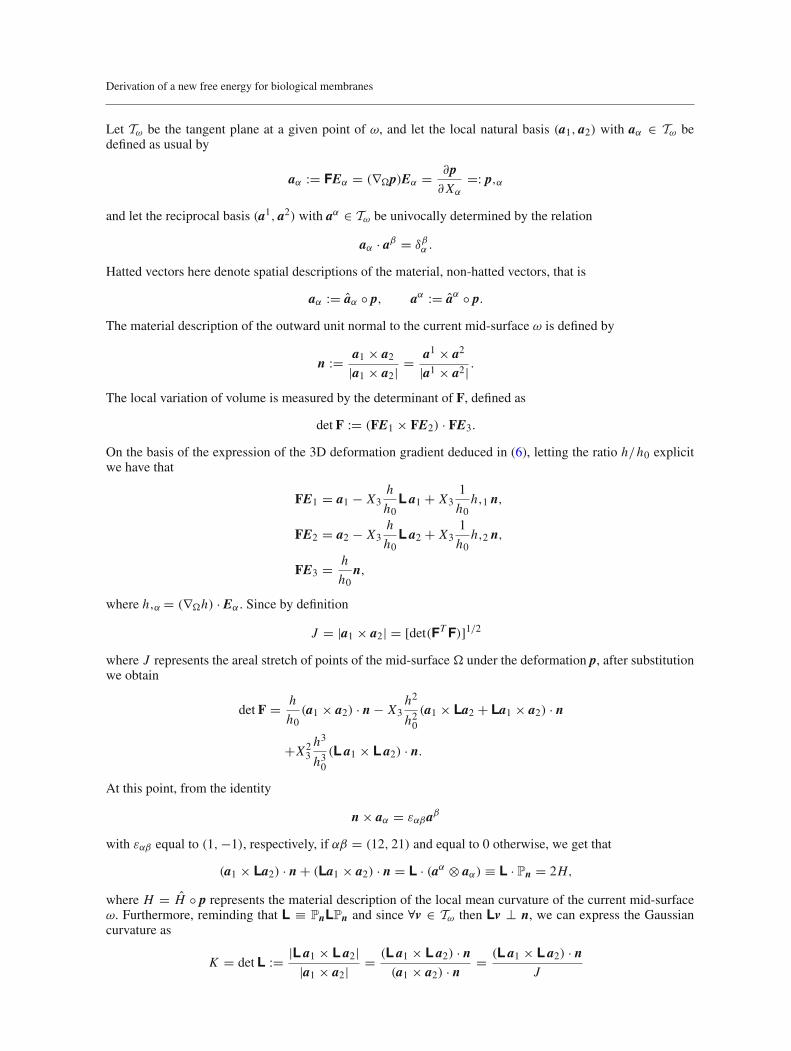
Let Tω be the tangent plane at a given point of ω, and let the local natural basis (a1, a2) with aα ∈ Tω bedefined as usual by

aα := FEα = (∇�p)Eα = ∂p∂Xα

=: p,α

and let the reciprocal basis (a1, a2) with aα ∈ Tω be univocally determined by the relation

aα · aβ = δβα .

Hatted vectors here denote spatial descriptions of the material, non-hatted vectors, that is

aα := aα ◦ p, aα := aα ◦ p.

The material description of the outward unit normal to the current mid-surface ω is defined by

n := a1 × a2

|a1 × a2| = a1 × a2

|a1 × a2| .

The local variation of volume is measured by the determinant of F, defined as

det F := (FE1 × FE2) · FE3.

On the basis of the expression of the 3D deformation gradient deduced in (6), letting the ratio h/h0 explicitwe have that

FE1 = a1 − X3h

h0L a1 + X3

1

h0h,1 n,

FE2 = a2 − X3h

h0L a2 + X3

1

h0h,2 n,

FE3 = h

h0n,

where h,α = (∇�h) · Eα . Since by definition

J = |a1 × a2| = [det(FT F)]1/2

where J represents the areal stretch of points of the mid-surface � under the deformation p, after substitutionwe obtain

det F = h

h0(a1 × a2) · n − X3

h2

h20

(a1 × La2 + La1 × a2) · n

+X23

h3

h30

(L a1 × L a2) · n.

At this point, from the identity

n × aα = εαβaβ

with εαβ equal to (1,−1), respectively, if αβ = (12, 21) and equal to 0 otherwise, we get that

(a1 × La2) · n + (La1 × a2) · n = L · (aα ⊗ aα) ≡ L · Pn = 2H,

where H = H ◦ p represents the material description of the local mean curvature of the current mid-surfaceω. Furthermore, reminding that L ≡ PnLPn and since ∀v ∈ Tω then Lv ⊥ n, we can express the Gaussiancurvature as

K = det L := |L a1 × L a2||a1 × a2| = (L a1 × L a2) · n

(a1 × a2) · n= (L a1 × L a2) · n

J

L. Deseri et al.

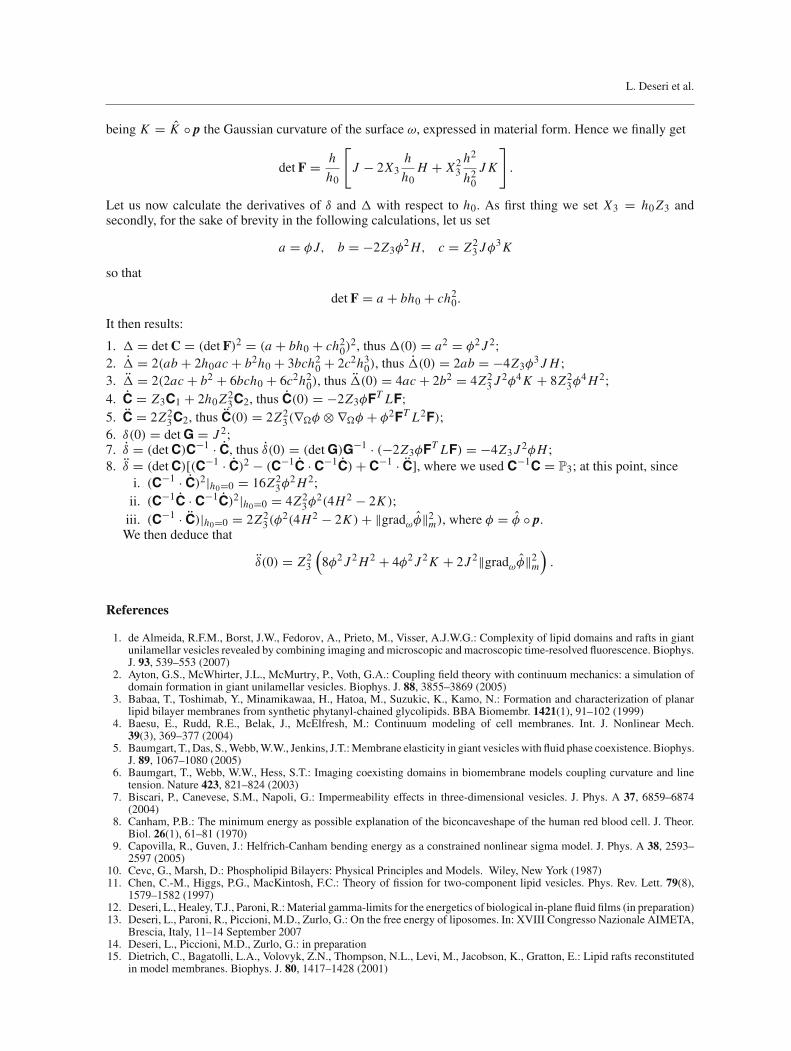
being K = K ◦ p the Gaussian curvature of the surface ω, expressed in material form. Hence we finally get

det F = h

h0

[

J − 2X3h

h0H + X2

3h2

h20

J K

]

.

Let us now calculate the derivatives of δ and with respect to h0. As first thing we set X3 = h0 Z3 andsecondly, for the sake of brevity in the following calculations, let us set

a = φ J, b = −2Z3φ2 H, c = Z2

3 Jφ3 K

so that

det F = a + bh0 + ch20.

It then results:

1. = det C = (det F)2 = (a + bh0 + ch20)

2, thus (0) = a2 = φ2 J 2;2. = 2(ab + 2h0ac + b2h0 + 3bch2

0 + 2c2h30), thus (0) = 2ab = −4Z3φ

3 J H ;3. = 2(2ac + b2 + 6bch0 + 6c2h2

0), thus (0) = 4ac + 2b2 = 4Z23 J 2φ4 K + 8Z2

3φ4 H2;

4. C = Z3C1 + 2h0 Z23C2, thus C(0) = −2Z3φFT LF;

5. C = 2Z23C2, thus C(0) = 2Z2

3(∇�φ ⊗ ∇�φ + φ2FT L2F);6. δ(0) = det G = J 2;7. δ = (det C)C−1 · C, thus δ(0) = (det G)G−1 · (−2Z3φFT LF) = −4Z3 J 2φH ;8. δ = (det C)[(C−1 · C)2 − (C−1C · C−1C)+ C−1 · C], where we used C−1C = P3; at this point, since

i. (C−1 · C)2|h0=0 = 16Z23φ

2 H2;ii. (C−1C · C−1C)2|h0=0 = 4Z2

3φ2(4H2 − 2K );

iii. (C−1 · C)|h0=0 = 2Z23(φ

2(4H2 − 2K )+ ‖gradωφ‖2m), where φ = φ ◦ p.

We then deduce that

δ(0) = Z23

(8φ2 J 2 H2 + 4φ2 J 2 K + 2J 2‖gradωφ‖2

m

).

References

1. de Almeida, R.F.M., Borst, J.W., Fedorov, A., Prieto, M., Visser, A.J.W.G.: Complexity of lipid domains and rafts in giantunilamellar vesicles revealed by combining imaging and microscopic and macroscopic time-resolved fluorescence. Biophys.J. 93, 539–553 (2007)

2. Ayton, G.S., McWhirter, J.L., McMurtry, P., Voth, G.A.: Coupling field theory with continuum mechanics: a simulation ofdomain formation in giant unilamellar vesicles. Biophys. J. 88, 3855–3869 (2005)

3. Babaa, T., Toshimab, Y., Minamikawaa, H., Hatoa, M., Suzukic, K., Kamo, N.: Formation and characterization of planarlipid bilayer membranes from synthetic phytanyl-chained glycolipids. BBA Biomembr. 1421(1), 91–102 (1999)

4. Baesu, E., Rudd, R.E., Belak, J., McElfresh, M.: Continuum modeling of cell membranes. Int. J. Nonlinear Mech.39(3), 369–377 (2004)

5. Baumgart, T., Das, S., Webb, W.W., Jenkins, J.T.: Membrane elasticity in giant vesicles with fluid phase coexistence. Biophys.J. 89, 1067–1080 (2005)

6. Baumgart, T., Webb, W.W., Hess, S.T.: Imaging coexisting domains in biomembrane models coupling curvature and linetension. Nature 423, 821–824 (2003)

7. Biscari, P., Canevese, S.M., Napoli, G.: Impermeability effects in three-dimensional vesicles. J. Phys. A 37, 6859–6874(2004)

8. Canham, P.B.: The minimum energy as possible explanation of the biconcaveshape of the human red blood cell. J. Theor.Biol. 26(1), 61–81 (1970)

9. Capovilla, R., Guven, J.: Helfrich-Canham bending energy as a constrained nonlinear sigma model. J. Phys. A 38, 2593–2597 (2005)

10. Cevc, G., Marsh, D.: Phospholipid Bilayers: Physical Principles and Models. Wiley, New York (1987)11. Chen, C.-M., Higgs, P.G., MacKintosh, F.C.: Theory of fission for two-component lipid vesicles. Phys. Rev. Lett. 79(8),

1579–1582 (1997)12. Deseri, L., Healey, T.J., Paroni, R.: Material gamma-limits for the energetics of biological in-plane fluid films (in preparation)13. Deseri, L., Paroni, R., Piccioni, M.D., Zurlo, G.: On the free energy of liposomes. In: XVIII Congresso Nazionale AIMETA,

Brescia, Italy, 11–14 September 200714. Deseri, L., Piccioni, M.D., Zurlo, G.: in preparation15. Dietrich, C., Bagatolli, L.A., Volovyk, Z.N., Thompson, N.L., Levi, M., Jacobson, K., Gratton, E.: Lipid rafts reconstituted

in model membranes. Biophys. J. 80, 1417–1428 (2001)


16. Do Carmo, M.P.: Differential Geometry of Curves and Surfaces. Prentice-Hall, New Jersey (1976)17. Erriu, G., Ladu, M., Onnis, S., Tang, J.H., Chang, W.K.: Modifications induced in lipid multilayers by 241Am-particles. Lett.

Al Nuovo Cimento Ser. 2 40(17), 527–532 (1984)18. Evans, E.A., Skalak, R.: Mechanics and Thermodynamics of Biomembranes. CRC Press, Boca Raton (1980)19. Fung, Y.C.: Theoretical considerations of the elasticity of red blood cells and small blood vessels. Proc. Fed. Am. Soc. Exp.

Biol. 25(6), 1761–1772 (1966)20. Fung, Y.C., Tong, P.: Theory of sphering of red blood cells. Biophys. J. 8, 175–198 (1968)21. Goldstein, R.E., Leibler, S.: Structural phase transitions of interacting membranes. Phys. Rev. A 40(2), 1025–1035 (1989)22. Gurtin, M.E.: An Introduction to Continuum Mechanics. Academic Press, New York (1981)23. Gurtin, M.E.: Configurational Forces as Basic Concepts of Continuum Physics. Springer, New York (2000)24. Gurtin, M.E., Murdoch, A.I.: Continuum theory of elastic material surfaces. Arch. Ration. Mech. Anal. 57(4), 291–323

(1975)25. Healey, T.J.: Phase transitions in giant unilamellar vescicles. Private communication (2007)26. Helfrich, W.: Elastic properties of lipid bilayers: theory and possible experiments. Z. Naturforsch [C] 28(11), 693–703

(1973)27. Hilgers, M.G., Pipkin, A.C.: Bending energy of highly elastic membranes. Q. Appl. Math. 50(2), 389–400 (1992)28. Hilgers, M.G., Pipkin, A.C.: Elastic sheets with bending stiffness. Q. J. Mech. Appl. Math. 45(1), 57–75 (1992)29. Hilgers, M.G., Pipkin, A.C.: Energy-minimizing deformations of elastic sheets with bending stiffness. J. Elast. 31(2),

125–139 (1993)30. Hill, T.: An Introduction to Statistical Thermodynamics. Dover, New York (1986)31. Israelachvili, J.N.: Intermolecular and Surface Forces. Academic Press, New York (1991)32. Julicher, F., Lipowsky, R.: Domain-induced budding of vesicles. Phys. Rev. E 70(19), 2964–2967 (1993)33. Julicher, F., Lipowsky, R.: Shape transformations of vesicles with intramembrane domains. Phys. Rev. E 53(3), 2670–2683

(1996)34. Kawakatsu, T., Andelman, A., Kawasaki, K., Taniguchi, T.: Phase transitions and shapes of two component membranes and

vesicles I: strong segregation limit. J. Physiol. II (France) 4(8), 1333–1362 (1994)35. Keller, J.B., Merchant, G.J.: Flexural rigidity of a liquid surface. J. Stat. Phys. 63(5-6), 1039–1051 (1991)36. Komura, S., Shirotori, H., Olmsted, P.D., Andelman, D.: Lateral phase separation in mixtures of lipids and cholesterol. Euro-

phys. Lett. 67, 321–327 (2004)37. Koiter, W.T.: On the nonlinear theory of thin elastic shells. Proc. K. Ned. Akad. Wet. B 69, 1–54 (1966)38. Lipowsky, R., Sackmann, E. (eds.): Handbook of Biological Physics—Structure and Dynamics of Membranes, vol. 1. Elsevier

Science B.V., Amsterdam (1995)39. Murdoch, A.I., Cohen, C.: Symmetry considerations for material surfaces. Arch. Ration. Mech. Anal. 72, 61–89 (1979)40. Nagle, J.: An overwiew and some insight on liposomes. Private communication, April (2005)41. Noll, W.: A mathematical theory of the mechanical behavior of continuous media. Arch. Ration. Mech. Anal. 2, 197–226

(1958)42. Onuki, A.: Phase Transition Dynamics. Cambridge University Press, Cambridge (2002)43. Ou-Yang, Z.C., Liu, J.X., Xie, Y.Z.: Geometric methods in the elastic theory of membranes in liquid cristal phases. World

Scientific, Singapore (1999)44. Rosso, R., Virga, E.G.: Squeezing and stretching of vesicles. J. Phys. A 33, 1459–1464 (2000)45. Safran, S.A.: Statistical Thermodynamics of Surfaces, Interfaces, and Membranes. Westview Press, Boulder (2003)46. Steigmann, D.J.: Fluid Films with curvature Elasticity. Arch. Ration. Mech. Anal. 150, 127–152 (1999)47. Steigmann, D.J.: Thin-plate theory for large elastic deformations. Int. J. Nonlinear Mech. 42(2), 233–240 (2007)48. Stottrup, B.L., Veatch, S.L., Keller, S.L.: Nonequilibrium behavior in supported lipid membranes containing cholesterol. Bio-

phys. J. 86, 2942–2950 (2004)49. Taniguchi, T.: Shape deformation and phase separation dynamics of two-component vesicles. Phys. Rev. Lett. 76(23), 4444–

4447 (1996)50. Tu, Z.C., Ou-Yang, Z.C.: Lipid membranes with free edges. Phys. Rev. E 68, 061915 (2003) [7 p.]51. Veatch, S.L., Keller, S.L.: Organization in lipid membranes containing cholesterol. Phys. Rev. Lett. 89(26), 268101-1–

268101-4 (2002)52. Veatch, S.L., Keller, S.L.: Letter to the editor: a closer look at the canonical “Raft Mixture” in model membrane studies. Bio-

phys. J. 84, 725–726 (2003)53. Veatch, S.L., Keller, S.L.: Separation of liquid phases in giant vesicles of ternary mixtures of phospholipids and choleste-

rol. Biophys. J. 85, 3074–3083 (2003)54. Veatch, S.L., Polozov, V.I., Gawrisch, K., Keller, S.L.: Liquid domains in vescicles investigated by NMR and fluorescence

microscopy. Biophys. J. 86, 2910–2922 (2004)55. Zurlo, G.: Material and geometric phase transitions in biological membranes. Dissertation for the Fulfillment of the Doctorate

of Philosophy in Structural Engineering and Continuum Mechanics [Deseri, L., Paroni, R., Marzano, S. (Advisors), Healey,T.J. (Co-Advisor)], University of Pisa (2006)

original article mario d. piccioni giuseppe zurlo ...deseril/publications/deseri piccioni...

Documents