prediction of moment redistribution in statically

applied sciences

Article

Prediction of Moment Redistribution in StaticallyIndeterminate Reinforced Concrete StructuresUsing Artificial Neural Network and SupportVector Regression

Ling Li 1,2,3, Wenzhong Zheng 1,2,3,* and Ying Wang 1,2,3

1 School of Civil Engineering, Harbin Institute of Technology, Harbin 150090, China;[email protected] (L.L.); [email protected] (Y.W.)

2 Key Lab of Structures Dynamic Behaviour and Control of the Ministry of Education,Harbin Institute of Technology, Harbin 150090, China

3 Key Lab of Smart Prevention and Mitigation of Civil Engineering Disasters of the Ministry of Industry andInformation Technology, Harbin Institute of Technology, Harbin 150090, China

* Correspondence: [email protected]; Tel.: +86-155-4501-4182

Received: 14 November 2018; Accepted: 19 December 2018; Published: 21 December 2018 ��

Abstract: In this paper, a new prediction model is proposed that fully considers the variousparameters influencing the moment redistribution in statically indeterminate reinforced concrete(RC) structures by using the artificial neural network (ANN) and support vector regression (SVR).Twenty-four continuous RC beams and 12 continuous RC frames with various design parameterswere tested to investigate the process of moment redistribution. Based on the experimental resultsobtained from this study and the published literature, a reliable database with 111 datasets wasdeveloped for the training and testing of the models. The predicted values of the proposed models,together with the estimations of the widely used code methods, were compared with the experimentalresults in the database. The analysis results showed that both the proposed ANN and SVR modelsexhibit high accuracy and reliability for the prediction of the moment redistribution.

Keywords: statically indeterminate RC structure; moment redistribution; artificial neural network;support vector regression; prediction

1. Introduction

Statically indeterminate reinforced concrete (RC) structures are some of the most commonstructural forms in engineering design. Owing to the cracking of the concrete, the strain penetration ofthe reinforcement, and the formation and gradual rotation of the plastic hinge regions, the relativestiffness of each cross section changes constantly during the loading process, which causes aredistribution of internal forces in the statically indeterminate structure. In structural design,the moment redistribution is considered since it can help to avoid the reinforcement congestion atcritical sections, thereby improving the convenience of the construction and the concreting conditions.Moreover, moment redistribution can help fully exploit the reserved capacity of the non-critical sectionsand achieve an economic design.

For practical applications, the current design codes allow designers to take advantage of linearelastic analysis with limit moment redistribution for structural design, in which the moment diagramderived from the elastic analysis of the structure is modified based on the degree of momentredistribution. Many definitions for measuring the moment redistribution have been proposed.

Appl. Sci. 2019, 9, 28; doi:10.3390/app9010028 www.mdpi.com/journal/applsci

http://www.mdpi.com/journal/applsci

http://www.mdpi.com

https://orcid.org/0000-0003-0824-1522

http://dx.doi.org/10.3390/app9010028

http://www.mdpi.com/journal/applsci

http://www.mdpi.com/2076-3417/9/1/28?type=check_update&version=4

Appl. Sci. 2019, 9, 28 2 of 24

The coefficient of the moment redistribution β, defined by Cohn [1] and adopted in various designcodes, is shown in Equation (1):

β =Melast −Mred

Melast(1)

where Melast is the elastic moment calculated by the elastic theory, Mred is the actual moment aftermoment redistribution, and β is between 0 and 1.

A reasonable consideration of the degree of the moment redistribution is important for theanalysis and design of structures. Traditionally, moment redistribution is considered to be heavilydependent on the ductile behavior of the critical section [2]. In most design provisions, momentredistribution is mainly related to the neutral axis depth factor (the ratio of neutral axis depth tothe section effective depth), since it can well characterize the ductility of a section by combining thecharacteristics of the materials and the geometry of the cross section. In fact, evaluation of the momentredistribution is complex because it depends on the rotation capacity of the plastic hinge as well asthe variation in the stiffness distribution and the bond between the reinforcement and concrete [3].Numerous studies have focused on the behavior and influencing factors of moment redistributionin statically indeterminate structures. Nearly all of these studies are based on a basic model ofcontinuous beams subjected to static loads. By using the concept of ductility demand, the effects ofvarious parameters, including slenderness, stiffness, ratio of tensile and compressive reinforcement,concrete strength, and strength of the reinforcement, on the moment redistribution in continuous RCbeams were studied by Scholz [4] and Mostofinejad et al. [5]. Based on the experiments of continuousRC beams, Bagge et al. [3] concluded that a decrease in the tensile reinforcement and increase inthe compression and transverse reinforcement would be beneficial for the moment redistribution.However, for high-strength concrete beams, the influence of the transverse reinforcement ratio is notsignificant, as observed in the experimental studies conducted by Carmo and Lopes [6]. Their studyalso indicated that the relationship between mid-span reinforcement ratio and intermediate-supportreinforcement ratio had a significant effect on moment redistribution. Scott et al. [7] experimentallystudied the whole process of the moment redistribution in continuous RC beams. Their resultsshow that the moment redistribution evolves through several stages and the parameters, such asthe cross-section size, concrete strength and arrangement of the reinforcement, affect the momentredistribution in each stage. In addition to the experimental studies, many theoretical methods havebeen proposed to investigate the effective behavior of continuous RC members. Oehlers et al. [8]developed a structural mechanics-based mathematical model for moment redistribution in continuousmembers, which was combined with the shear-friction approach [9], partial-interaction theory [10],and rigid body displacement. Through the application of this model, they concluded that momentredistribution increased with the decrease in the bond strength and the increase in the diameter ofsteel bars and concrete confinement. To study the entire nonlinear behavior of RC continuous beams, afinite element model based on the moment–curvature relationship and the Timoshenko beam theorywas established by Lou et al. [11]. By using this model, the effect of many factors, such as the concretestrength, the relationship between the tensile reinforcement ratios at critical negative and positivemoment regions, the relative stiffness, and the concrete confinement on moment redistribution werestudied comprehensively.

As mentioned above, the mechanics of moment redistribution are incredibly complicated. The aimof this study was to propose a new model for accurate prediction of the moment redistribution thatconsiders the various influential parameters as comprehensively as possible, while being convenient forthe applications of practical engineering. In recent years, artificial intelligence techniques of artificialneural networks (ANNs) and support vector machines (SVMs) have exhibited great potential forsolving various problems in civil engineering. Different from most methods used in civil engineering,ANN and SVM algorithms do not rely on the existing theories about structural mechanism, but employhigh precision fitting to match the results to the real values as closely as possible [12]. These twomodels have been successfully applied to several areas in structural engineering, such as structural

Appl. Sci. 2019, 9, 28 3 of 24

analysis [13–15], prediction of the shear resistance in beams [16–19] and compressive strength ofcolumns [20–23], displacement determination of RC buildings [24], and estimation of the compressivestrength for various types of concrete [25–29]. More recently, they were used to understand the behaviorof structures under extreme conditions. Based on a back-propagation ANN, Ince [30] developed afracture model to predict the fracture parameters of cementitious materials. Compared with thecommon non-linear fracture mechanics approaches, the ANN model was more reliable. In a separatestudy, Erdem [31] established an ANN model for determining the ultimate moment capacity of RCslabs in fire. The prediction values were compared with the results provided by the ultimate momentcapacity equation, which showed the ANN model had a high degree of accuracy. To ensure the realisticfire performance of steel structures, Naser [32] used ANN to derive temperature-dependent thermaland mechanical material models for structural steel. The applicability of the models was validatedusing numerical case studies with a highly nonlinear finite element model. The results indicated thatthe proposed ANN models can significantly enhance the current state of structural fire design bydeveloping a uniform representation of material properties at elevated temperatures.

However, few studies have focused on the prediction of the moment redistribution in the staticallyindeterminate RC structures using artificial intelligence techniques. In this paper, an experimentalstudy on the moment redistribution in 24 continuous RC beams and 12 continuous RC frames withvarious design parameters was presented. Furthermore, two models of ANN and SVM were developedusing MATLAB software (MathWorks, Neddick, MA, USA) to predict the coefficient of momentredistribution in the statically RC indeterminate structures. In total, 111 experimental datasets weregathered to construct the models and a description of the development procedure is provided here.The main influential factors, including the neutral axis depth factor (c/d), the ratio of the tensilereinforcement ratio over the critical negative moment regions to the tensile reinforcement ratio over thepositive moment regions (ρs1/ρs2), the yield strength of the reinforcement (f y), the concrete compressivestrength (f c’), the slenderness ratio (l/h), the effective depth of the section (h0), the stirrup ratio (ωw),and the loading form, were used as input parameters to the models. Finally, the new proposed modelswere verified against the experimental results and compared with the provisions in the design codesto assess their accuracy and reliability.

2. Experimental Database

As the first step in developing the ANN and SVR models, a comprehensive set of experimentaldata on the moment redistribution was required for the training and testing samples. The databaseused in this paper was established by collecting the datasets from the experiments conducted in thecurrent test and the relevant experimental programs in previous studies [3,6,7,33–37].

2.1. Experimental Program

2.1.1. Test Scheme

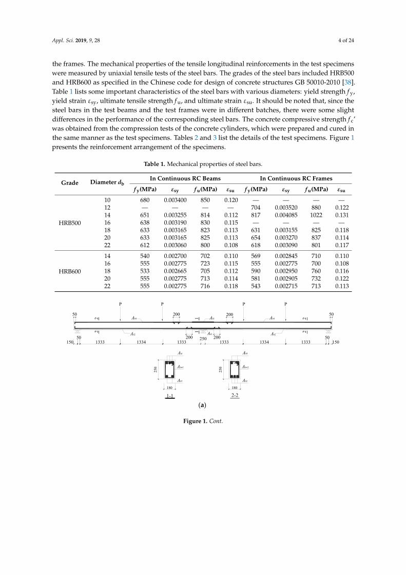
A total of 24 two-span continuous RC beams and 12 single-layer two-span continuous RC frameswere designed and tested to investigate the moment redistribution at the negative moment regions.The rectangular cross-section of the continuous beams and frame beams were 180 mm × 250 mm and180 mm× 300 mm, respectively. The length of each span of the continuous beams and frame beams are4 m and 3 m, respectively. Owing to the limited number of test specimens, four main variables affectingthe moment redistribution were considered in the design, namely, the neutral axis depth factor (c/d),the ratio of the tensile reinforcement ratio over the critical negative moment regions to the tensilereinforcement ratio over the positive moment regions (ρs1/ρs2), the yield strength of the reinforcement(f y), and the concrete compressive strength (f c’). All beams were designed to have a reserve capacity inthe positive moment regions, which ensure that the internal forces transfer from the negative momentregions to the positive moment regions. A sufficient magnitude of stirrups was arranged in all beamsto avoid shear failure, and the strong column–weak beam requirement was followed in the design of

Appl. Sci. 2019, 9, 28 4 of 24

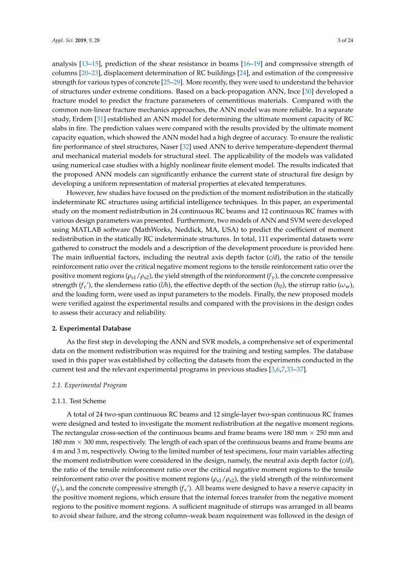
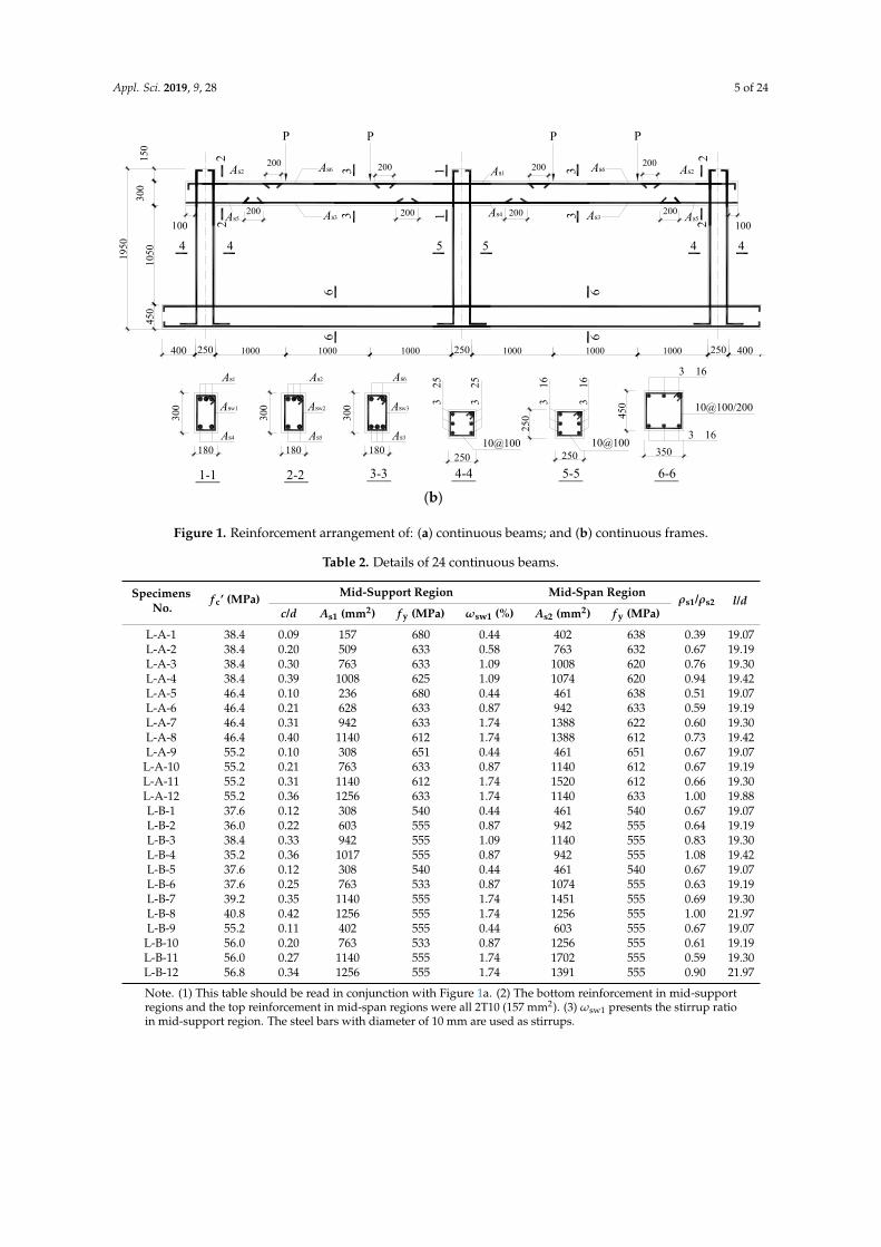
the frames. The mechanical properties of the tensile longitudinal reinforcements in the test specimenswere measured by uniaxial tensile tests of the steel bars. The grades of the steel bars included HRB500and HRB600 as specified in the Chinese code for design of concrete structures GB 50010-2010 [38].Table 1 lists some important characteristics of the steel bars with various diameters: yield strength f y,yield strain εsy, ultimate tensile strength f u, and ultimate strain εsu. It should be noted that, since thesteel bars in the test beams and the test frames were in different batches, there were some slightdifferences in the performance of the corresponding steel bars. The concrete compressive strength f c’was obtained from the compression tests of the concrete cylinders, which were prepared and cured inthe same manner as the test specimens. Tables 2 and 3 list the details of the test specimens. Figure 1presents the reinforcement arrangement of the specimens.

Table 1. Mechanical properties of steel bars.

Grade Diameter dbIn Continuous RC Beams In Continuous RC Frames

f y(MPa) εsy f u(MPa) εsu f y(MPa) εsy f u(MPa) εsu

HRB500

10 680 0.003400 850 0.120 — — — —12 — — — — 704 0.003520 880 0.12214 651 0.003255 814 0.112 817 0.004085 1022 0.13116 638 0.003190 830 0.115 — — — —18 633 0.003165 823 0.113 631 0.003155 825 0.11820 633 0.003165 825 0.113 654 0.003270 837 0.11422 612 0.003060 800 0.108 618 0.003090 801 0.117

HRB600

14 540 0.002700 702 0.110 569 0.002845 710 0.11016 555 0.002775 723 0.115 555 0.002775 700 0.10818 533 0.002665 705 0.112 590 0.002950 760 0.11620 555 0.002775 713 0.114 581 0.002905 732 0.12222 555 0.002775 716 0.118 543 0.002715 713 0.113

Appl. Sci. 2018, 8, x FOR PEER REVIEW 4 of 25

grades of the steel bars included HRB500 and HRB600 as specified in the Chinese code for design of concrete structures GB 50010-2010 [38]. Table 1 lists some important characteristics of the steel bars with various diameters: yield strength fy, yield strain εsy, ultimate tensile strength fu, and ultimate strain εsu. It should be noted that, since the steel bars in the test beams and the test frames were in different batches, there were some slight differences in the performance of the corresponding steel bars. The concrete compressive strength fc’ was obtained from the compression tests of the concrete cylinders, which were prepared and cured in the same manner as the test specimens. Tables 2 and 3 list the details of the test specimens. Figure 1 presents the reinforcement arrangement of the specimens.

Table 1. Mechanical properties of steel bars.

Grade Diameter db In Continuous RC Beams In Continuous RC Frames fy(MPa) εsy fu(MPa) εsu fy(MPa) εsy fu(MPa) εsu

HRB500

10 680 0.003400 850 0.120 — — — — 12 — — — — 704 0.003520 880 0.122 14 651 0.003255 814 0.112 817 0.004085 1022 0.131 16 638 0.003190 830 0.115 — — — — 18 633 0.003165 823 0.113 631 0.003155 825 0.118 20 633 0.003165 825 0.113 654 0.003270 837 0.114 22 612 0.003060 800 0.108 618 0.003090 801 0.117

HRB600

14 540 0.002700 702 0.110 569 0.002845 710 0.110 16 555 0.002775 723 0.115 555 0.002775 700 0.108 18 533 0.002665 705 0.112 590 0.002950 760 0.116 20 555 0.002775 713 0.114 581 0.002905 732 0.122 22 555 0.002775 716 0.118 543 0.002715 713 0.113

(a)

50 200

15050

1333 1334

P P

1333200

As2

As4

22

11

As1

As3

Asw1

As4

As2

Asw2

250

180

250

180

50200

15050

13331334

PP

1333200

As1

As2

As4

22

250As3

1-1 2-2

Figure 1. Cont.

Appl. Sci. 2019, 9, 28 5 of 24Appl. Sci. 2018, 8, x FOR PEER REVIEW 5 of 25

(b)

Figure 1. Reinforcement arrangement of: (a) continuous beams; and (b) continuous frames.

Table 2. Details of 24 continuous beams.

Specimens No. fc’ (MPa) Mid-Support Region

Mid-Span Region ρs1/ρs2 l/d

c/d As1 (mm2) fy (MPa) ωsw1 (%)

As2 (mm2) fy (MPa)

L-A-1 38.4 0.09 157 680 0.44

402 638 0.39 19.07

L-A-2 38.4 0.20 509 633 0.58

763 632 0.67 19.19

L-A-3 38.4 0.30 763 633 1.09

1008 620 0.76 19.30

L-A-4 38.4 0.39 1008 625 1.09

1074 620 0.94 19.42

L-A-5 46.4 0.10 236 680 0.44

461 638 0.51 19.07

L-A-6 46.4 0.21 628 633 0.87

942 633 0.59 19.19

L-A-7 46.4 0.31 942 633 1.74

1388 622 0.60 19.30

L-A-8 46.4 0.40 1140 612 1.74

1388 612 0.73 19.42

L-A-9 55.2 0.10 308 651 0.44

461 651 0.67 19.07

L-A-10 55.2 0.21 763 633 0.87

1140 612 0.67 19.19

L-A-11 55.2 0.31 1140 612 1.74

1520 612 0.66 19.30

L-A-12 55.2 0.36 1256 633 1.74

1140 633 1.00 19.88

L-B-1 37.6 0.12 308 540 0.44

461 540 0.67 19.07

L-B-2 36.0 0.22 603 555 0.87

942 555 0.64 19.19

L-B-3 38.4 0.33 942 555 1.09

1140 555 0.83 19.30

L-B-4 35.2 0.36 1017 555 0.87

942 555 1.08 19.42

L-B-5 37.6 0.12 308 540 0.44

461 540 0.67 19.07

L-B-6 37.6 0.25 763 533 0.87

1074 555 0.63 19.19

L-B-7 39.2 0.35 1140 555 1.74

1451 555 0.69 19.30

L-B-8 40.8 0.42 1256 555 1.74

1256 555 1.00 21.97

L-B-9 55.2 0.11 402 555 0.44

603 555 0.67 19.07

3 13

3 13

1011001200

4 4

3

150

450

1050

300

400 250

1950

100

3

5

2501000 1000 1000

2

33 1

2

1

P P

As2

As5 As3

As3

200

200

200

200

1-1

As1

As4

Asw1

300

180

3-3

As3

As3

Asw3

300

180

2-2

As2

As5

Asw2

300

180

4-4

325

101100

5-5 3-3250

250

250

450

350

325

313

313

101100

44

3

400250

100

3

100010001000

2

33

2

PP

As1

As4

As2

As5As3

As3

200

200

200

200

5

Figure 1. Reinforcement arrangement of: (a) continuous beams; and (b) continuous frames.

Table 2. Details of 24 continuous beams.

SpecimensNo.

f c’ (MPa) Mid-Support Region Mid-Span Regionρs1/ρs2 l/d

c/d As1 (mm2) f y (MPa) ωsw1 (%) As2 (mm2) f y (MPa)

L-A-1 38.4 0.09 157 680 0.44 402 638 0.39 19.07L-A-2 38.4 0.20 509 633 0.58 763 632 0.67 19.19L-A-3 38.4 0.30 763 633 1.09 1008 620 0.76 19.30L-A-4 38.4 0.39 1008 625 1.09 1074 620 0.94 19.42L-A-5 46.4 0.10 236 680 0.44 461 638 0.51 19.07L-A-6 46.4 0.21 628 633 0.87 942 633 0.59 19.19L-A-7 46.4 0.31 942 633 1.74 1388 622 0.60 19.30L-A-8 46.4 0.40 1140 612 1.74 1388 612 0.73 19.42L-A-9 55.2 0.10 308 651 0.44 461 651 0.67 19.07L-A-10 55.2 0.21 763 633 0.87 1140 612 0.67 19.19L-A-11 55.2 0.31 1140 612 1.74 1520 612 0.66 19.30L-A-12 55.2 0.36 1256 633 1.74 1140 633 1.00 19.88L-B-1 37.6 0.12 308 540 0.44 461 540 0.67 19.07L-B-2 36.0 0.22 603 555 0.87 942 555 0.64 19.19L-B-3 38.4 0.33 942 555 1.09 1140 555 0.83 19.30L-B-4 35.2 0.36 1017 555 0.87 942 555 1.08 19.42L-B-5 37.6 0.12 308 540 0.44 461 540 0.67 19.07L-B-6 37.6 0.25 763 533 0.87 1074 555 0.63 19.19L-B-7 39.2 0.35 1140 555 1.74 1451 555 0.69 19.30L-B-8 40.8 0.42 1256 555 1.74 1256 555 1.00 21.97L-B-9 55.2 0.11 402 555 0.44 603 555 0.67 19.07

L-B-10 56.0 0.20 763 533 0.87 1256 555 0.61 19.19L-B-11 56.0 0.27 1140 555 1.74 1702 555 0.59 19.30L-B-12 56.8 0.34 1256 555 1.74 1391 555 0.90 21.97

Note. (1) This table should be read in conjunction with Figure 1a. (2) The bottom reinforcement in mid-supportregions and the top reinforcement in mid-span regions were all 2T10 (157 mm2). (3) ωsw1 presents the stirrup ratioin mid-support region. The steel bars with diameter of 10 mm are used as stirrups.

Appl. Sci. 2019, 9, 28 6 of 24

Table 3. Details of 12 frame beams.

SpecimensNo.

f c’(MPa)

Mid-Support Region End-Support Region Mid-SpanRegion

ρs1/ρs3 ρs2/ρs3 l/d

c/d As1(mm2)

f y(MPa)

ωsw1(%) c/d As2

(mm2)f y

(MPa)ωsw2(%)

As3(mm2)

f y(MPa)

KL-A-1 36.8 0.29 823 638 1.57 0.10 226 704 1.26 1140 618 0.72 0.20 11.54KL-A-2 38.4 0.38 1140 618 2.51 0.17 461 817 1.57 1256 654 0.91 0.34 11.54KL-A-3 50.4 0.27 1008 654 2.51 0.10 308 817 1.57 1140 618 0.82 0.25 11.54KL-A-4 52.0 0.36 1256 654 2.51 0.13 461 817 2.51 1520 618 0.83 0.28 11.54KL-A-5 54.4 0.28 1140 618 2.51 0.09 308 817 2.51 1388 636 0.82 0.20 11.54KL-A-6 56.0 0.39 1520 618 2.51 0.13 509 631 2.51 1570 654 0.97 0.30 11.54KL-B-1 35.2 0.32 942 581 1.57 0.10 308 569 1.26 942 581 1.00 0.33 11.54KL-B-2 40.0 0.41 1256 581 2.51 0.15 509 590 1.57 1388 562 0.84 0.34 11.54KL-B-3 50.4 0.26 1140 543 2.51 0.10 402 555 1.57 1388 562 0.82 0.29 11.54KL-B-4 46.4 0.41 1520 543 2.51 0.13 509 590 2.51 1520 543 1.00 0.31 11.54KL-B-5 47.2 0.38 1388 562 2.51 0.09 308 569 1.57 1388 562 0.92 0.20 11.54KL-B-6 55.2 0.41 1702 581 2.51 0.14 628 590 2.51 2281 543 0.75 0.25 11.54

Note: (1) This table should be read in conjunction with Figure 1b. (2) The top reinforcement in mid-span regions,the bottom reinforcement in mid-support regions and end-support regions are all 2T10 (157 mm2). (3) ωsw1 andωsw2 presents the stirrup ratio in mid-support and end-support region, respectively. The steel bars with diameter of12 mm are used as stirrups.

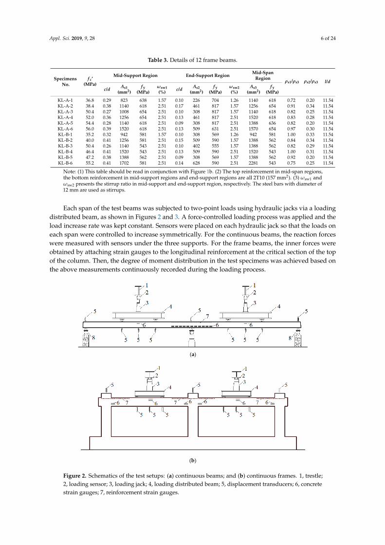
Each span of the test beams was subjected to two-point loads using hydraulic jacks via a loadingdistributed beam, as shown in Figures 2 and 3. A force-controlled loading process was applied and theload increase rate was kept constant. Sensors were placed on each hydraulic jack so that the loads oneach span were controlled to increase symmetrically. For the continuous beams, the reaction forceswere measured with sensors under the three supports. For the frame beams, the inner forces wereobtained by attaching strain gauges to the longitudinal reinforcement at the critical section of the topof the column. Then, the degree of moment distribution in the test specimens was achieved based onthe above measurements continuously recorded during the loading process.


L-B-10 56.0 0.20 763 533 0.87

1256 555 0.61 19.19

L-B-11 56.0 0.27 1140 555 1.74

1702 555 0.59 19.30

L-B-12 56.8 0.34 1256 555 1.74

1391 555 0.90 21.97

Note. (1) This table should be read in conjunction with Figure 1a. (2) The bottom reinforcement in mid-support regions and

the top reinforcement in mid-span regions were all 2T10 (157 mm2). (3) ωsw1 presents the stirrup ratio in mid-support region.

The steel bars with diameter of 10 mm are used as stirrups.

Table 3. Details of 12 frame beams.

Specimens No.

fc’ (MPa)

Mid-Support Region

End-Support Region

Mid-Span Region

ρs1/ρs3 ρs2/ρs3 l/d c/d

As1

(mm2) fy

(MPa) ωsw1

(%)

c/d As2

(mm2) fy

(MPa) ωsw2

(%)

As3

(mm2) fy (MPa)

KL-A-1 36.8 0.29 823 638 1.57

0.10 226 704 1.26

1140 618 0.72 0.20 11.54

KL-A-2 38.4 0.38 1140 618 2.51

0.17 461 817 1.57

1256 654 0.91 0.34 11.54

KL-A-3 50.4 0.27 1008 654 2.51

0.10 308 817 1.57

1140 618 0.82 0.25 11.54

KL-A-4 52.0 0.36 1256 654 2.51

0.13 461 817 2.51

1520 618 0.83 0.28 11.54

KL-A-5 54.4 0.28 1140 618 2.51

0.09 308 817 2.51

1388 636 0.82 0.20 11.54

KL-A-6 56.0 0.39 1520 618 2.51

0.13 509 631 2.51

1570 654 0.97 0.30 11.54

KL-B-1 35.2 0.32 942 581 1.57

0.10 308 569 1.26

942 581 1.00 0.33 11.54

KL-B-2 40.0 0.41 1256 581 2.51

0.15 509 590 1.57

1388 562 0.84 0.34 11.54

KL-B-3 50.4 0.26 1140 543 2.51

0.10 402 555 1.57

1388 562 0.82 0.29 11.54

KL-B-4 46.4 0.41 1520 543 2.51

0.13 509 590 2.51

1520 543 1.00 0.31 11.54

KL-B-5 47.2 0.38 1388 562 2.51

0.09 308 569 1.57

1388 562 0.92 0.20 11.54

KL-B-6 55.2 0.41 1702 581 2.51

0.14 628 590 2.51

2281 543 0.75 0.25 11.54 Note: (1) This table should be read in conjunction with Figure 1b. (2) The top reinforcement in mid-span regions, the bottom

reinforcement in mid-support regions and end-support regions are all 2T10 (157 mm2). (3) ωsw1 and ωsw2 presents the stirrup ratio in mid-support and end-support region, respectively. The steel bars with diameter of 12 mm are used as stirrups.

Each span of the test beams was subjected to two-point loads using hydraulic jacks via a loading distributed beam, as shown in Figures 2 and 3. A force-controlled loading process was applied and the load increase rate was kept constant. Sensors were placed on each hydraulic jack so that the loads on each span were controlled to increase symmetrically. For the continuous beams, the reaction forces were measured with sensors under the three supports. For the frame beams, the inner forces were obtained by attaching strain gauges to the longitudinal reinforcement at the critical section of the top of the column. Then, the degree of moment distribution in the test specimens was achieved based on the above measurements continuously recorded during the loading process.

(a)


(b)

1, trestle; 2, loading sensor; 3, loading jack; 4, loading distributed beam; 5, displacement transducers; 6, concrete strain gauges; 7, reinforcement strain gauges.

Figure 2. Schematics of the test setups: (a) continuous beams; and (b) continuous frames.

(a) (b)

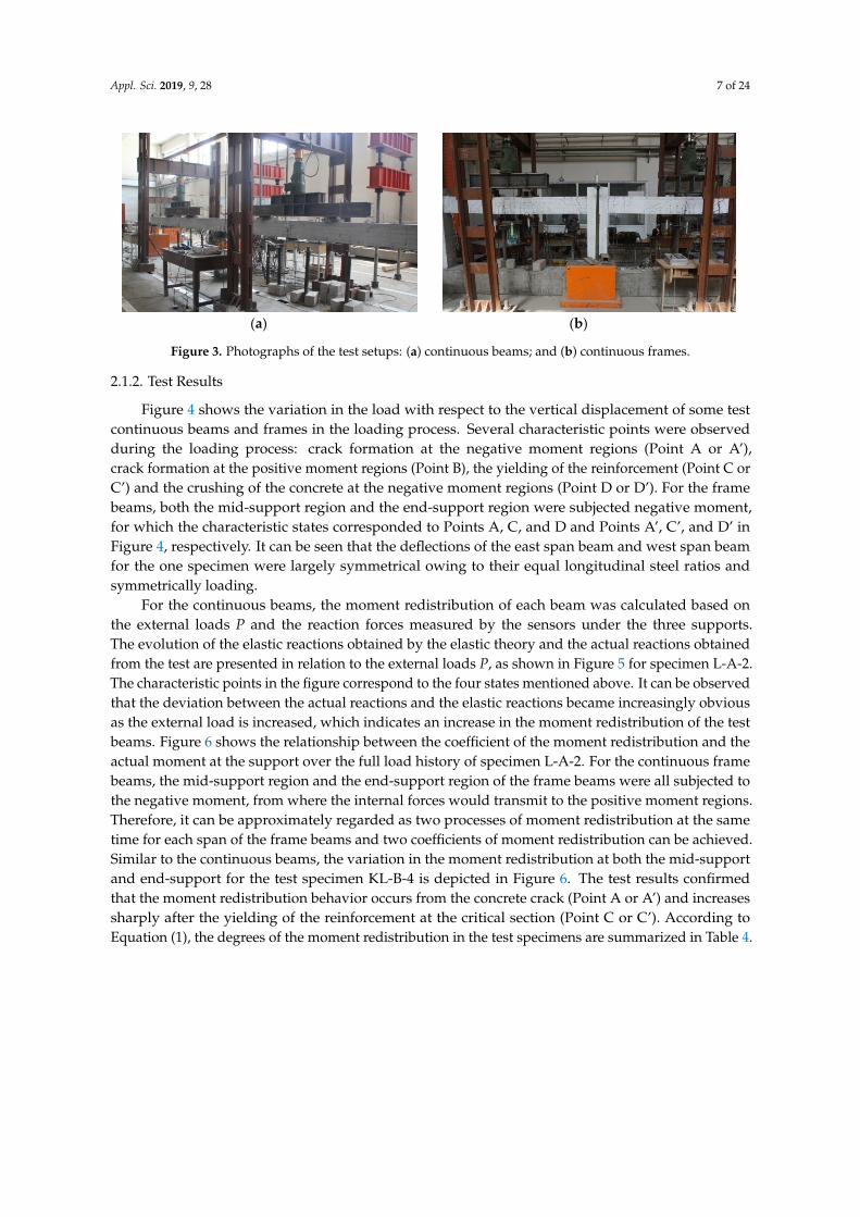
Figure 3. Photographs of the test setups: (a) continuous beams; and (b) continuous frames.

2.1.2. Test Results

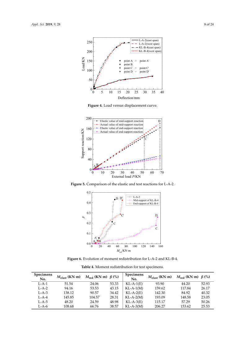
Figure 4 shows the variation in the load with respect to the vertical displacement of some test continuous beams and frames in the loading process. Several characteristic points were observed during the loading process: crack formation at the negative moment regions (Point A or A’), crack formation at the positive moment regions (Point B), the yielding of the reinforcement (Point C or C’) and the crushing of the concrete at the negative moment regions (Point D or D’). For the frame beams, both the mid-support region and the end-support region were subjected negative moment, for which the characteristic states corresponded to Points A, C, and D and Points A’, C’, and D’ in Figure 4, respectively. It can be seen that the deflections of the east span beam and west span beam for the one specimen were largely symmetrical owing to their equal longitudinal steel ratios and symmetrically loading.

For the continuous beams, the moment redistribution of each beam was calculated based on the external loads P and the reaction forces measured by the sensors under the three supports. The evolution of the elastic reactions obtained by the elastic theory and the actual reactions obtained from the test are presented in relation to the external loads P, as shown in Figure 5 for specimen L-A-2. The characteristic points in the figure correspond to the four states mentioned above. It can be observed that the deviation between the actual reactions and the elastic reactions became increasingly

Figure 2. Schematics of the test setups: (a) continuous beams; and (b) continuous frames. 1, trestle;2, loading sensor; 3, loading jack; 4, loading distributed beam; 5, displacement transducers; 6, concretestrain gauges; 7, reinforcement strain gauges.

Appl. Sci. 2019, 9, 28 7 of 24


(b)

1, trestle; 2, loading sensor; 3, loading jack; 4, loading distributed beam; 5, displacement transducers; 6, concrete strain gauges; 7, reinforcement strain gauges.

Figure 2. Schematics of the test setups: (a) continuous beams; and (b) continuous frames.

(a) (b)


2.1.2. Test Results

Figure 4 shows the variation in the load with respect to the vertical displacement of some test continuous beams and frames in the loading process. Several characteristic points were observed during the loading process: crack formation at the negative moment regions (Point A or A’), crack formation at the positive moment regions (Point B), the yielding of the reinforcement (Point C or C’) and the crushing of the concrete at the negative moment regions (Point D or D’). For the frame beams, both the mid-support region and the end-support region were subjected negative moment, for which the characteristic states corresponded to Points A, C, and D and Points A’, C’, and D’ in Figure 4, respectively. It can be seen that the deflections of the east span beam and west span beam for the one specimen were largely symmetrical owing to their equal longitudinal steel ratios and symmetrically loading.

For the continuous beams, the moment redistribution of each beam was calculated based on the external loads P and the reaction forces measured by the sensors under the three supports. The evolution of the elastic reactions obtained by the elastic theory and the actual reactions obtained from the test are presented in relation to the external loads P, as shown in Figure 5 for specimen L-A-2. The characteristic points in the figure correspond to the four states mentioned above. It can be observed that the deviation between the actual reactions and the elastic reactions became increasingly


2.1.2. Test Results

Figure 4 shows the variation in the load with respect to the vertical displacement of some testcontinuous beams and frames in the loading process. Several characteristic points were observedduring the loading process: crack formation at the negative moment regions (Point A or A’),crack formation at the positive moment regions (Point B), the yielding of the reinforcement (Point C orC’) and the crushing of the concrete at the negative moment regions (Point D or D’). For the framebeams, both the mid-support region and the end-support region were subjected negative moment,for which the characteristic states corresponded to Points A, C, and D and Points A’, C’, and D’ inFigure 4, respectively. It can be seen that the deflections of the east span beam and west span beamfor the one specimen were largely symmetrical owing to their equal longitudinal steel ratios andsymmetrically loading.

For the continuous beams, the moment redistribution of each beam was calculated based onthe external loads P and the reaction forces measured by the sensors under the three supports.The evolution of the elastic reactions obtained by the elastic theory and the actual reactions obtainedfrom the test are presented in relation to the external loads P, as shown in Figure 5 for specimen L-A-2.The characteristic points in the figure correspond to the four states mentioned above. It can be observedthat the deviation between the actual reactions and the elastic reactions became increasingly obviousas the external load is increased, which indicates an increase in the moment redistribution of the testbeams. Figure 6 shows the relationship between the coefficient of the moment redistribution and theactual moment at the support over the full load history of specimen L-A-2. For the continuous framebeams, the mid-support region and the end-support region of the frame beams were all subjected tothe negative moment, from where the internal forces would transmit to the positive moment regions.Therefore, it can be approximately regarded as two processes of moment redistribution at the sametime for each span of the frame beams and two coefficients of moment redistribution can be achieved.Similar to the continuous beams, the variation in the moment redistribution at both the mid-supportand end-support for the test specimen KL-B-4 is depicted in Figure 6. The test results confirmedthat the moment redistribution behavior occurs from the concrete crack (Point A or A’) and increasessharply after the yielding of the reinforcement at the critical section (Point C or C’). According toEquation (1), the degrees of the moment redistribution in the test specimens are summarized in Table 4.

Appl. Sci. 2019, 9, 28 8 of 24


obvious as the external load is increased, which indicates an increase in the moment redistribution of the test beams. Figure 6 shows the relationship between the coefficient of the moment redistribution and the actual moment at the support over the full load history of specimen L-A-2. For the continuous frame beams, the mid-support region and the end-support region of the frame beams were all subjected to the negative moment, from where the internal forces would transmit to the positive moment regions. Therefore, it can be approximately regarded as two processes of moment redistribution at the same time for each span of the frame beams and two coefficients of moment redistribution can be achieved. Similar to the continuous beams, the variation in the moment redistribution at both the mid-support and end-support for the test specimen KL-B-4 is depicted in Figure 6. The test results confirmed that the moment redistribution behavior occurs from the concrete crack (Point A or A’) and increases sharply after the yielding of the reinforcement at the critical section (Point C or C’). According to Equation (1), the degrees of the moment redistribution in the test specimens are summarized in Table 4.

0 5 10 15 20 25 30 35 400

50

100

150

200

250

point A point A' point B point C point C' point D point D'Lo

ad1K

N

Deflection1mm

L-A-2(east span) L-A-2(west span) KL-B-4(east span) KL-B-4(west span)

Figure 4. Load versus displacement curve.

0 10 20 30 40 50 30 700

40

80

120

130

200

BA

Supp

ort r

eact

ion1

KN

External load P1KN

Elastic value of mid-support reactionActual value of mid-support reactionElastic value of end-support reactionActual value of end-support reaction

C

D

0 20 40 30 80 100 120 140 1300.0

0.1

0.2

0.3

0.4

0.5

A'

D D'

D

C

C'

C

BA

L-A-2 Mid-support of KL-B-4 End-support of KL-B-4

β

Mred1KN·m

Figure 5. Comparison of the elastic and test reactions for L-A-2.

Figure 6. Evolution of moment redistribution for L-A-2 and KL-B-4.

Table 4. Moment redistribution for test specimens.

Specimens No.

)mKN(elast ⋅M )mKN(red ⋅M β(%) Specimens

No. )mKN(elast ⋅M )mKN(red ⋅M β(%)

L-A-1 51.54 24.06 53.33 KL-A-1(E) 93.90 44.20 52.93 L-A-2 94.16 53.53 43.15 KL-A-1(M) 159.62 117.84 26.17 L-A-3 138.12 90.57 34.42 KL-A-2(E) 142.30 84.92 40.32 L-A-4 145.85 104.57 28.31 KL-A-2(M) 193.09 148.58 23.05 L-A-5 48.20 24.59 48.98 KL-A-3(E) 115.17 57.29 50.26




0 5 10 15 20 25 30 35 400

50

100

150

200

250


ad1K

N

Deflection1mm



0 10 20 30 40 50 30 700

40

80

120

130

200

BA

Supp

ort r

eact

ion1

KN

External load P1KN


C

D

0 20 40 30 80 100 120 140 1300.0

0.1

0.2

0.3

0.4

0.5

A'

D D'

D

C

C'

C

BA


β Mred1KN·m




Specimens No.







0 5 10 15 20 25 30 35 400

50

100

150

200

250


ad1K

N

Deflection1mm



0 10 20 30 40 50 30 700

40

80

120

130

200

BA

Supp

ort r

eact

ion1

KN

External load P1KN


C

D

0 20 40 30 80 100 120 140 1300.0

0.1

0.2

0.3

0.4

0.5

A'

D D'

D

C

C'

C

BA


β

Mred1KN·m




Specimens No.






SpecimensNo. Melast (KN·m) Mred (KN·m) β (%) Specimens

No. Melast (KN·m) Mred (KN·m) β (%)

L-A-1 51.54 24.06 53.33 KL-A-1(E) 93.90 44.20 52.93L-A-2 94.16 53.53 43.15 KL-A-1(M) 159.62 117.84 26.17L-A-3 138.12 90.57 34.42 KL-A-2(E) 142.30 84.92 40.32L-A-4 145.85 104.57 28.31 KL-A-2(M) 193.09 148.58 23.05L-A-5 48.20 24.59 48.98 KL-A-3(E) 115.17 57.29 50.26L-A-6 108.68 66.76 38.57 KL-A-3(M) 206.27 153.62 25.53

Appl. Sci. 2019, 9, 28 9 of 24

Table 4. Cont.

SpecimensNo. Melast (KN·m) Mred (KN·m) β (%) Specimens

No. Melast (KN·m) Mred (KN·m) β (%)

L-A-7 137.24 91.16 33.58 KL-A-4(E) 160.55 84.37 47.45L-A-8 122.46 87.78 28.32 KL-A-4(M) 206.19 153.10 25.75L-A-9 60.86 33.13 45.57 KL-A-5(E) 140.14 55.04 60.73

L-A-10 142.12 91.56 35.57 KL-A-5(M) 228.79 159.87 30.13L-A-11 124.48 89.59 28.03 KL-A-6(E) 126.08 75.45 40.16L-A-12 115.36 84.75 26.53 KL-A-6(M) 235.89 190.73 19.14L-B-1 63.94 32.82 48.65 KL-B-1(E) 79.81 40.75 48.94L-B-2 95.06 52.86 44.39 KL-B-1(M) 147.00 110.20 25.03L-B-3 116.01 75.85 34.61 KL-B-2(E) 114.62 67.64 40.98L-B-4 102.36 68.93 32.67 KL-B-2(M) 181.09 139.00 23.24L-B-5 50.59 27.32 45.99 KL-B-3(E) 115.17 53.57 53.49L-B-6 107.48 68.15 36.60 KL-B-3(M) 190.43 140.17 26.39L-B-7 128.80 87.85 31.79 KL-B-4(E) 132.61 72.39 45.41L-B-8 136.79 95.00 30.55 KL-B-4(M) 206.27 151.13 26.73L-B-9 78.18 42.40 45.76 KL-B-5(E) 126.53 49.92 60.54L-B-10 110.15 70.92 35.61 KL-B-5(M) 200.19 146.91 26.61L-B-11 136.79 96.44 29.50 KL-B-6(E) 137.60 89.67 34.83L-B-12 124.79 85.26 31.68 KL-B-6(M) 225.61 189.98 15.79

Note: The letters E and M in the “specimens No.”, respectively, indicate the end-support and mid-support of theframe beams.

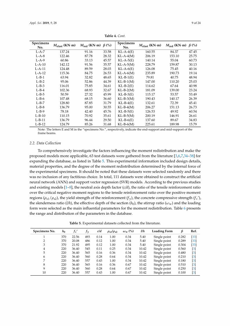
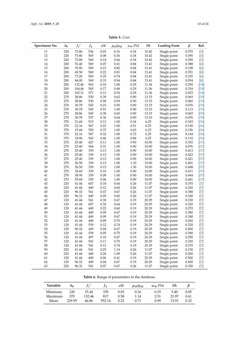
2.2. Data Collection

To comprehensively investigate the factors influencing the moment redistribution and make theproposed models more applicable, 63 test datasets were gathered from the literature [3,6,7,34–38] forexpanding the database, as listed in Table 5. This experimental information included design details,material properties, and the degree of the moment redistribution determined by the internal force ofthe experimental specimens. It should be noted that these datasets were selected randomly and therewas no inclusion of any factitious choice. In total, 111 datasets were obtained to construct the artificialneural network (ANN) and support vector regression (SVR) models. According to the previous studiesand existing models [1–8], the neutral axis depth factor (c/d), the ratio of the tensile reinforcement ratioover the critical negative moment regions to the tensile reinforcement ratio over the positive momentregions (ρs1/ρs2), the yield strength of the reinforcement (f y), the concrete compressive strength (f c’),the slenderness ratio (l/h), the effective depth of the section (h0), the stirrup ratio (ωw) and the loadingform were selected as the main influential parameters for the moment redistribution. Table 6 presentsthe range and distribution of the parameters in the database.

Table 5. Experimental datasets collected from the literature.

Specimens No. h0 f c’ f y c/d ρs1/ρs2 ωw (%) l/h Loading Form β Ref.

1 370 22.56 493 0.14 1.00 0.34 5.40 Single point 0.282 [33]2 370 20.08 486 0.12 1.00 0.34 5.40 Single point 0.289 [33]3 370 21.92 495 0.12 1.00 0.34 5.40 Single point 0.304 [33]4 220 36.40 545 0.11 0.25 0.34 10.42 Single point 0.560 [3]5 220 36.40 565 0.16 0.36 0.34 10.42 Single point 0.480 [3]6 220 36.40 560 0.28 0.64 0.34 10.42 Single point 0.210 [3]7 220 36.40 557 0.43 1.00 0.34 10.42 Single point 0.180 [3]8 220 36.40 565 0.16 0.36 0.67 10.42 Single point 0.510 [3]9 220 36.40 560 0.28 0.64 0.67 10.42 Single point 0.250 [3]

10 220 36.40 557 0.43 1.00 0.67 10.42 Single point 0.100 [3]

Appl. Sci. 2019, 9, 28 10 of 24

Table 5. Cont.

Specimens No. h0 f c’ f y c/d ρs1/ρs2 ωw (%) l/h Loading Form β Ref.

11 220 73.80 536 0.03 0.16 0.34 10.42 Single point 0.570 [3]12 220 73.80 565 0.08 0.36 0.34 10.42 Single point 0.390 [3]13 220 73.80 560 0.14 0.64 0.34 10.42 Single point 0.290 [3]14 200 76.40 569 0.07 0.41 0.84 13.41 Single point 0.388 [6]15 200 70.90 569 0.15 0.82 0.84 13.41 Single point 0.158 [6]16 200 69.50 569 0.22 0.81 0.84 13.41 Single point 0.351 [6]17 200 73.20 569 0.29 0.74 0.84 13.41 Single point 0.105 [6]18 200 84.00 569 0.33 0.94 0.84 13.41 Single point 0.054 [6]19 200 132.46 563 0.18 1.00 0.29 11.36 Single point 0.250 [34]20 200 104.46 565 0.17 0.68 0.29 11.36 Single point 0.318 [34]21 200 102.31 571 0.13 0.54 0.29 11.36 Single point 0.453 [34]22 270 28.86 530 0.39 0.62 0.90 13.33 Single point 0.065 [35]23 270 28.86 530 0.58 0.94 0.90 13.33 Single point 0.060 [35]24 270 30.78 545 0.23 0.50 0.90 13.33 Single point 0.076 [35]25 270 30.78 545 0.51 1.00 0.90 13.33 Single point 0.113 [35]26 270 28.86 545 0.38 0.60 0.90 13.33 Single point 0.065 [35]27 270 30.78 537 0.30 0.64 0.90 13.33 Single point 0.076 [35]28 370 21.68 515 0.13 1.00 0.34 6.25 Single point 0.183 [36]29 370 22.16 567 0.22 1.00 0.51 6.25 Single point 0.150 [36]30 370 15.44 550 0.37 1.00 0.63 6.25 Single point 0.156 [36]31 370 22.16 567 0.32 1.00 0.72 6.25 Single point 0.144 [36]32 370 18.96 543 0.46 1.00 0.84 6.25 Single point 0.110 [36]33 270 25.40 427 0.11 1.00 0.90 10.00 Single point 0.352 [37]34 270 25.40 564 0.31 1.00 0.90 10.00 Single point 0.076 [37]35 270 25.40 339 0.13 1.00 0.90 10.00 Single point 0.413 [37]36 270 25.40 339 0.13 1.00 0.90 10.00 Single point 0.423 [37]37 270 25.40 339 0.13 1.00 0.90 10.00 Single point 0.421 [37]38 270 26.50 339 0.13 1.00 1.10 10.00 Single point 0.401 [37]39 270 26.50 339 0.13 1.00 1.30 10.00 Single point 0.448 [37]40 270 34.60 339 0.10 1.00 0.90 10.00 Single point 0.411 [37]41 270 38.90 339 0.09 1.00 0.90 10.00 Single point 0.444 [37]42 270 55.60 339 0.06 1.00 0.90 10.00 Single point 0.441 [37]43 220 41.44 607 0.18 0.64 0.26 11.07 Single point 0.370 [7]44 220 41.44 449 0.12 0.60 0.26 11.07 Single point 0.320 [7]45 220 96.32 541 0.07 0.67 0.26 11.07 Single point 0.380 [7]46 220 96.32 449 0.05 0.60 0.26 11.07 Single point 0.340 [7]47 120 41.44 541 0.30 0.67 0.19 20.29 Single point 0.230 [7]48 120 41.44 607 0.32 0.64 0.19 20.29 Single point 0.320 [7]49 120 41.44 449 0.22 0.60 0.19 20.29 Single point 0.270 [7]50 120 41.44 449 0.09 0.67 0.19 20.29 Single point 0.380 [7]51 120 41.44 449 0.09 0.67 0.19 20.29 Single point 0.340 [7]52 120 41.44 449 0.09 0.70 0.19 20.29 Single point 0.260 [7]53 120 41.44 539 0.12 0.74 0.19 20.29 Single point 0.220 [7]54 120 96.32 449 0.04 0.67 0.19 20.29 Single point 0.400 [7]55 120 41.44 539 0.05 0.75 0.19 20.29 Single point 0.390 [7]56 120 41.44 497 0.10 0.67 0.19 20.29 Single point 0.250 [7]57 120 41.44 541 0.11 0.70 0.19 20.29 Single point 0.320 [7]58 120 41.44 541 0.12 0.74 0.19 20.29 Single point 0.270 [7]59 220 41.44 541 0.25 1.14 0.26 11.07 Single point 0.130 [7]60 220 41.44 449 0.20 1.09 0.26 11.07 Single point 0.200 [7]61 120 41.44 449 0.06 0.41 0.19 20.29 Single point 0.500 [7]62 120 96.32 449 0.04 0.67 0.19 20.29 Single point 0.450 [7]63 220 96.32 541 0.07 0.67 0.26 11.07 Single point 0.330 [7]

Table 6. Range of parameters in the database.

Variable h0 f c’ f y c/d ρs1/ρs2 ωw (%) l/h β

Minimum 120 15.44 339 0.03 0.16 0.19 5.40 0.05Maximum 370 132.46 817 0.58 1.14 2.51 21.97 0.61

Mean 229.95 46.86 552.14 0.22 0.71 0.99 13.91 0.32

Appl. Sci. 2019, 9, 28 11 of 24

3. Modeling Method

3.1. Artificial Neural Networks

The ANN is an information processing system that simulates the structure and functional featuresof the biological nervous system. It consists of a large number of highly interconnected processingelements (neurons), and their inherent laws can be obtained by the training of the input parameters,which leads to a strong nonlinear mapping ability [39].

3.1.1. Neural Network Architecture

The multilayer feed-forward back propagation network (MFBPN), first proposed byRumerlhar et al. in 1986 [40], is one of the most commonly used ANN methods due to its simplestructure and strong plasticity. The MFBPN is composed of three main parts: an input layer, one ormore hidden layers and an output layer. All neurons in each layer are connected to the neurons in thenext layer by network weights and biases. The values of the neuron received from the lower layer aremultiplied by the specific weights and then summed with the bias. The sum is processed by predefinedactivation functions and transferred to the next layer, as follows:

yj = f (netj) = f (n

∑i=1

wijxi + bj) (2)

where netj is the weighted sum for the jth neuron, xi is the input values of the ith neuron in the lowerlayer, wij is the weight between the ith neuron and the jth neuron, bj is the bias value of the jth neuronand f is the activation function. In the present work, sigmoid activations were used in each layer.

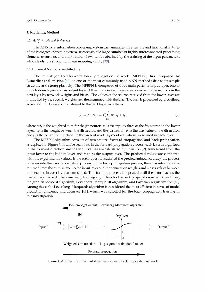
The MFBPN algorithm consists of two stages: forward propagation and back propagation,as depicted in Figure 7. It can be seen that, in the forward propagation process, each layer is organizedin the forward direction and the input values are calculated by Equation (2), transferred from theinput layer to the hidden layer and then to the output layer. The predicted values are comparedwith the experimental values. If the error does not satisfied the predetermined accuracy, the processreverses into the back propagation process. In the back propagation process, the error information isreturned from the output layer to the input layer and the connection weights and biases values betweenthe neurons in each layer are modified. This training process is repeated until the error reaches thedesired requirement. There are many training algorithms for the back propagation network, includingthe gradient descent algorithm, Levenberg–Marquardt algorithm, and Bayesian regularization [40].Among these, the Levenberg–Marquardt algorithm is considered the most efficient in terms of modelprediction efficiency and accuracy [41], which was selected for the back propagation training inthis investigation.Appl. Sci. 2018, 8, x FOR PEER REVIEW 12 of 25

Figure 7. Architecture of the multilayer feed-forward back propagation network.

3.1.2. Construction of Neural Network

In this study, the collected experimental data of the moment redistribution coefficient were randomly divided into a training set and a testing set. Since the purposes in different experimental studies are diverse and the test programs are time-consuming and costly, datasets with complete variable information collected from the published literature are relatively few. To improve the applicability and generalization of the training model, 85% of the data were selected as training data, which were used to fit the parameters of the neural network, such as the weights and the bias in each layer. The remaining 15% of the data were used as testing data, which were independent of the training process and used to test the accuracy and applicability of the trained model.

The performance of the neural network models can be evaluated by two indexes: mean squared error (MSE) and coefficient of correlation (R2), as given by Equations (3) and (4):

=

−=n

iii ct

n 1

2)(1MSE (3)

=

=

−

−−= n

ii

n

iii

tt

ctR

1

2

1

2

2

)(

)(1 (4)

where n is the total number of the data, ci and ti are the predicted value and the target value of the ith data, and t is the average of the target values. A prediction model is considered to be better fitting when MSE and R2 are closer to 0 and 1, respectively.

Eight nodes were used in the input layer because there were eight influential parameters for the moment redistribution studied. Before training the input data, normalizations for the input and target data should be performed since the sigmoid activation function is sensitive to the variations between 0 and 1. In this way, the stability and convergence rate of the training process can be improved. A linear relationship was used to scale the data from 0.1 to 0.9, given by Equation (5):

1.01.09.0minmax

minscaled, +

−−×−=

xxxxx i

i ）（ (5)

where xi,scaled is the normalized value, xi is the value of the variable, and xmin and xmax are the minimum and maximum values of the variable, respectively.

The function of the hidden layer is to determine the inherent relationship between the input and output layers based on the training of the data. One hidden layer was used in the present neural network. The number of the nodes in the hidden layer is of great importance to the design of the neural network. An excessive number of the nodes results in an extension of the training time and

Input I net=∑wijxi+bj

0

-1

1

O=f (net)

[w]

[b]

Output O

Log-sigmoid activation functionWeighted sum function

Forward propagation

Back propagation with Levenberg-Marquardt algorithm

Figure 7. Architecture of the multilayer feed-forward back propagation network.

Appl. Sci. 2019, 9, 28 12 of 24

3.1.2. Construction of Neural Network

In this study, the collected experimental data of the moment redistribution coefficient wererandomly divided into a training set and a testing set. Since the purposes in different experimentalstudies are diverse and the test programs are time-consuming and costly, datasets with completevariable information collected from the published literature are relatively few. To improve theapplicability and generalization of the training model, 85% of the data were selected as trainingdata, which were used to fit the parameters of the neural network, such as the weights and the bias ineach layer. The remaining 15% of the data were used as testing data, which were independent of thetraining process and used to test the accuracy and applicability of the trained model.

The performance of the neural network models can be evaluated by two indexes: mean squarederror (MSE) and coefficient of correlation (R2), as given by Equations (3) and (4):

MSE =1n

n

∑i=1

(ti − ci)2 (3)

R2 = 1−

n∑

i=1(ti − ci)

2

n∑

i=1(ti − t)2

(4)

where n is the total number of the data, ci and ti are the predicted value and the target value of the ithdata, and t is the average of the target values. A prediction model is considered to be better fittingwhen MSE and R2 are closer to 0 and 1, respectively.

Eight nodes were used in the input layer because there were eight influential parameters for themoment redistribution studied. Before training the input data, normalizations for the input and targetdata should be performed since the sigmoid activation function is sensitive to the variations between 0and 1. In this way, the stability and convergence rate of the training process can be improved. A linearrelationship was used to scale the data from 0.1 to 0.9, given by Equation (5):

xi,scaled = (0.9− 0.1)× xi − xmin

xmax − xmin+ 0.1 (5)

where xi,scaled is the normalized value, xi is the value of the variable, and xmin and xmax are theminimum and maximum values of the variable, respectively.

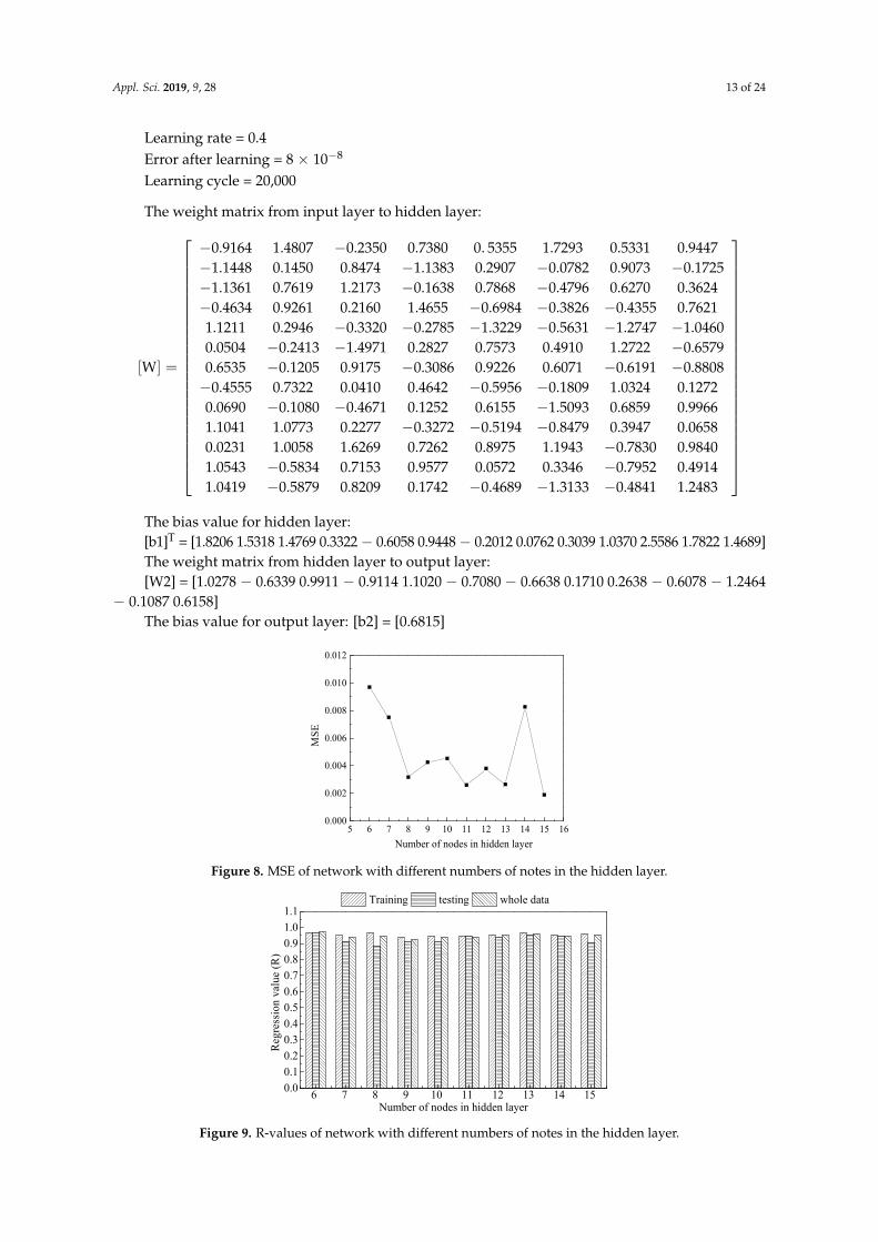
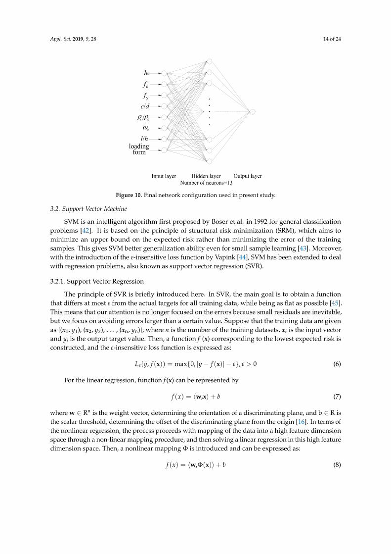
The function of the hidden layer is to determine the inherent relationship between the input andoutput layers based on the training of the data. One hidden layer was used in the present neuralnetwork. The number of the nodes in the hidden layer is of great importance to the design of theneural network. An excessive number of the nodes results in an extension of the training time andthe over-fitting of the data, which decreases the computational efficiency. However, if the number ofthe nodes is not enough, insufficient information leads to a decrease in the computational accuracy.Currently, there are no general rules to exactly determine the number of nodes. It is often based onexperience, and the optimum result is obtained through trial and error. In this study, the number ofthe nodes in the hidden layer was selected from 6 to 15. Figures 8 and 9 show the regression valuesand MSE of the neural network with different numbers of nodes. It can be seen that the model isoptimal when 13 nodes were used in the hidden layer. Hence, the final network configuration used inpresent study is illustrated in Figure 10 and the values of the parameters for the neural network weredetermined as follows:

Number of input layer units = 8Number of hidden layer units = 13Number of output layer units = 1Momentum rate = 0.9

Appl. Sci. 2019, 9, 28 13 of 24

Learning rate = 0.4Error after learning = 8 × 10−8

Learning cycle = 20,000

The weight matrix from input layer to hidden layer:

[W] =

−0.9164 1.4807 −0.2350 0.7380 0. 5355 1.7293 0.5331 0.9447−1.1448 0.1450 0.8474 −1.1383 0.2907 −0.0782 0.9073 −0.1725−1.1361 0.7619 1.2173 −0.1638 0.7868 −0.4796 0.6270 0.3624−0.4634 0.9261 0.2160 1.4655 −0.6984 −0.3826 −0.4355 0.76211.1211 0.2946 −0.3320 −0.2785 −1.3229 −0.5631 −1.2747 −1.04600.0504 −0.2413 −1.4971 0.2827 0.7573 0.4910 1.2722 −0.65790.6535 −0.1205 0.9175 −0.3086 0.9226 0.6071 −0.6191 −0.8808−0.4555 0.7322 0.0410 0.4642 −0.5956 −0.1809 1.0324 0.12720.0690 −0.1080 −0.4671 0.1252 0.6155 −1.5093 0.6859 0.99661.1041 1.0773 0.2277 −0.3272 −0.5194 −0.8479 0.3947 0.06580.0231 1.0058 1.6269 0.7262 0.8975 1.1943 −0.7830 0.98401.0543 −0.5834 0.7153 0.9577 0.0572 0.3346 −0.7952 0.49141.0419 −0.5879 0.8209 0.1742 −0.4689 −1.3133 −0.4841 1.2483

The bias value for hidden layer:[b1]T = [1.8206 1.5318 1.4769 0.3322− 0.6058 0.9448− 0.2012 0.0762 0.3039 1.0370 2.5586 1.7822 1.4689]The weight matrix from hidden layer to output layer:[W2] = [1.0278 − 0.6339 0.9911 − 0.9114 1.1020 − 0.7080 − 0.6638 0.1710 0.2638 − 0.6078 − 1.2464

− 0.1087 0.6158]The bias value for output layer: [b2] = [0.6815]Appl. Sci. 2018, 8, x FOR PEER REVIEW 14 of 25

5 3 7 8 9 10 11 12 13 14 15 130.000

0.002

0.004

0.003

0.008

0.010

0.012

MSE

Number of nodes in hidden layer Figure 8. MSE of network with different numbers of notes in the hidden layer.

3 7 8 9 10 11 12 13 14 150.00.10.20.30.40.50.30.70.80.91.01.1

Regr

essio

n va

lue

(R)

Number of nodes in hidden layer

Training testing whole data

Figure 9. R-values of network with different numbers of notes in the hidden layer.

Figure 10. Final network configuration used in present study.

3.2. Support Vector Machine

SVM is an intelligent algorithm first proposed by Boser et al. in 1992 for general classification problems [42]. It is based on the principle of structural risk minimization (SRM), which aims to minimize an upper bound on the expected risk rather than minimizing the error of the training

h0

f 'cfy

c1dρs1 ρs21

ωw

l1hloading

form

Input layer Hidden layerNumber of neurons=13

Output layer

Figure 8. MSE of network with different numbers of notes in the hidden layer.


5 3 7 8 9 10 11 12 13 14 15 130.000

0.002

0.004

0.003

0.008

0.010

0.012

MSE


3 7 8 9 10 11 12 13 14 150.00.10.20.30.40.50.30.70.80.91.01.1

Regr

essio

n va

lue

(R)







h0

f 'cfy

c1dρs1 ρs21

ωw

l1hloading

form


Output layer


Appl. Sci. 2019, 9, 28 14 of 24


5 3 7 8 9 10 11 12 13 14 15 130.000

0.002

0.004

0.003

0.008

0.010

0.012

MSE


3 7 8 9 10 11 12 13 14 150.00.10.20.30.40.50.30.70.80.91.01.1

Regr

essio

n va

lue

(R)







h0

f 'cfy

c1dρs1 ρs21

ωw

l1hloading

form


Output layer



SVM is an intelligent algorithm first proposed by Boser et al. in 1992 for general classificationproblems [42]. It is based on the principle of structural risk minimization (SRM), which aims tominimize an upper bound on the expected risk rather than minimizing the error of the trainingsamples. This gives SVM better generalization ability even for small sample learning [43]. Moreover,with the introduction of the ε-insensitive loss function by Vapink [44], SVM has been extended to dealwith regression problems, also known as support vector regression (SVR).

3.2.1. Support Vector Regression

The principle of SVR is briefly introduced here. In SVR, the main goal is to obtain a functionthat differs at most ε from the actual targets for all training data, while being as flat as possible [45].This means that our attention is no longer focused on the errors because small residuals are inevitable,but we focus on avoiding errors larger than a certain value. Suppose that the training data are givenas {(x1, y1), (x2, y2), . . . , (xn, yn)}, where n is the number of the training datasets, xi is the input vectorand yi is the output target value. Then, a function f (x) corresponding to the lowest expected risk isconstructed, and the ε-insensitive loss function is expressed as:

Lε(y, f (x)) = max{0, |y− f (x)| − ε}, ε > 0 (6)

For the linear regression, function f (x) can be represented by

f (x) = 〈w,x〉+ b (7)

where w ∈ Rn is the weight vector, determining the orientation of a discriminating plane, and b ∈ R isthe scalar threshold, determining the offset of the discriminating plane from the origin [16]. In terms ofthe nonlinear regression, the process proceeds with mapping of the data into a high feature dimensionspace through a non-linear mapping procedure, and then solving a linear regression in this high featuredimension space. Then, a nonlinear mapping Φ is introduced and can be expressed as:

f (x) = 〈w,Φ(x)〉+ b (8)

Appl. Sci. 2019, 9, 28 15 of 24

To ensure the flatness of Equation (8), a smaller value of w is required. In real problems, it isimpossible for all data points to have an error lesser than ε for the one function. For this reason, the slackvariables ξi and ξi

* are introduced. Therefore, the SVR can be formulated as an optimization problem:

Minimize12‖w‖2 + C

n

∑i=1

(ξi + ξ∗i ) subjected to

yi − 〈w, Φ(xi)〉 − b ≤ ε + ξi〈w, Φ(xi)〉+ b− yi ≤ ε + ξ∗iξi, ξ∗i ≥ 0

(9)

where C is the regularized constant specified by the user. It is defined as the penalty factor to indicatethe trade-off between the flatness of the function and the empirical error.

The optimization problem in Equation (9) can be solved by introducing the Lagrangianmultipliers αi, α∗i , ηi, η∗i and the above optimization problem can be transformed into a dual quadraticprogramming problem:

Maximizing− 12

n∑

i=1

n∑

j=1(αi − α∗i )(αj − α∗j )K(xi, xj)−ε

n∑

i=1(αi + α∗i ) +

n∑

i=1yi(αi − α∗i )

Subjected ton∑

i=1(αi − α∗i ) = 0 and αi, α∗i ∈ [0, C]

(10)

where K(xi, xj) = Φ(xi)·Φ(xj) is defined as the kernel function, which is an important analysistechnique in SVR. The values of αi and α∗i can be obtained by solving Equation (10), and the functionf (x) is finally written as:

f (x) =n

∑i=1

(αi − α∗i )K(xi, xj) + b (11)

3.2.2. Construction of SVR Model

As discussed above, the SVR model is constructed by optimizing the ε-insensitive loss function,in which the parameter ε and the regularized constant C are the important optimization factors.Furthermore, the selection of the kernel function is also closely related to the SVR model performance.The commonly used kernel functions in the regression include the linear kernel function, polynomialkernel function, radial basis function (RBF), and sigmoid kernel function. Considering the infinitedimensional feature space corresponding to the RBF, the following RBF is adopted in this study:

K(xi, xj) = e−‖xi−xj‖

2

σ2 = e−g‖xi−xj‖2(12)

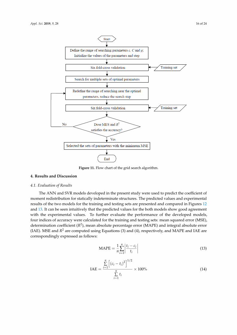
where σ indicates the smoothness of the derived function and g = 1/σ2 is the key parameter of the RBF.To select the optimal values of the parameters ε, C, and g involved in the SVR model, a grid

search algorithm was used in the present study. The basic idea of the grid search algorithm is totry every possible value of the parameters in a certain space with a specified step distance, and theparameters that optimize the performance of the SVR model with the best accuracy can be derivedbased on the cross-validation [46]. The process of the algorithm is illustrated through a flowchart, asshown in Figure 11. Similar to the construction of the neural network in Section 3.1.2., the collectedexperimental data of the moment redistribution coefficient were divided into two sets (85% for trainingand 15% for testing) for SVR. To increase the efficiency of the SVR training, the input and target datawere normalized within the range of 0.1 to 0.9, in accordance with Equation (5), before the training ofthe input data. Based on the grid search algorithm and a six-fold cross-validation, the values of theparameters for the SVR were determined as follows: ε = 0.01, C = 20, and g = 0.03.

Appl. Sci. 2019, 9, 28 16 of 24


3.2.2. Construction of SVR Model

As discussed above, the SVR model is constructed by optimizing the ε-insensitive loss function, in which the parameter ε and the regularized constant C are the important optimization factors. Furthermore, the selection of the kernel function is also closely related to the SVR model performance. The commonly used kernel functions in the regression include the linear kernel function, polynomial kernel function, radial basis function (RBF), and sigmoid kernel function. Considering the infinite dimensional feature space corresponding to the RBF, the following RBF is adopted in this study:

22

2

),( ji

jig

ji eeK xxxx

xx −−−

−== σ (12)

where σ indicates the smoothness of the derived function and g = 1 σ2⁄ is the key parameter of the RBF.

To select the optimal values of the parameters ε, C, and g involved in the SVR model, a grid search algorithm was used in the present study. The basic idea of the grid search algorithm is to try every possible value of the parameters in a certain space with a specified step distance, and the parameters that optimize the performance of the SVR model with the best accuracy can be derived based on the cross-validation [46]. The process of the algorithm is illustrated through a flowchart, as shown in Figure 11. Similar to the construction of the neural network in Section 3.1.2., the collected experimental data of the moment redistribution coefficient were divided into two sets (85% for training and 15% for testing) for SVR. To increase the efficiency of the SVR training, the input and target data were normalized within the range of 0.1 to 0.9, in accordance with Equation (5), before the training of the input data. Based on the grid search algorithm and a six-fold cross-validation, the values of the parameters for the SVR were determined as follows: ε = 0.01, C = 20, and g = 0.03.

Figure 11. Flow chart of the grid search algorithm.

4. Results and Discussion

Figure 11. Flow chart of the grid search algorithm.

4. Results and Discussion

4.1. Evaluation of Results

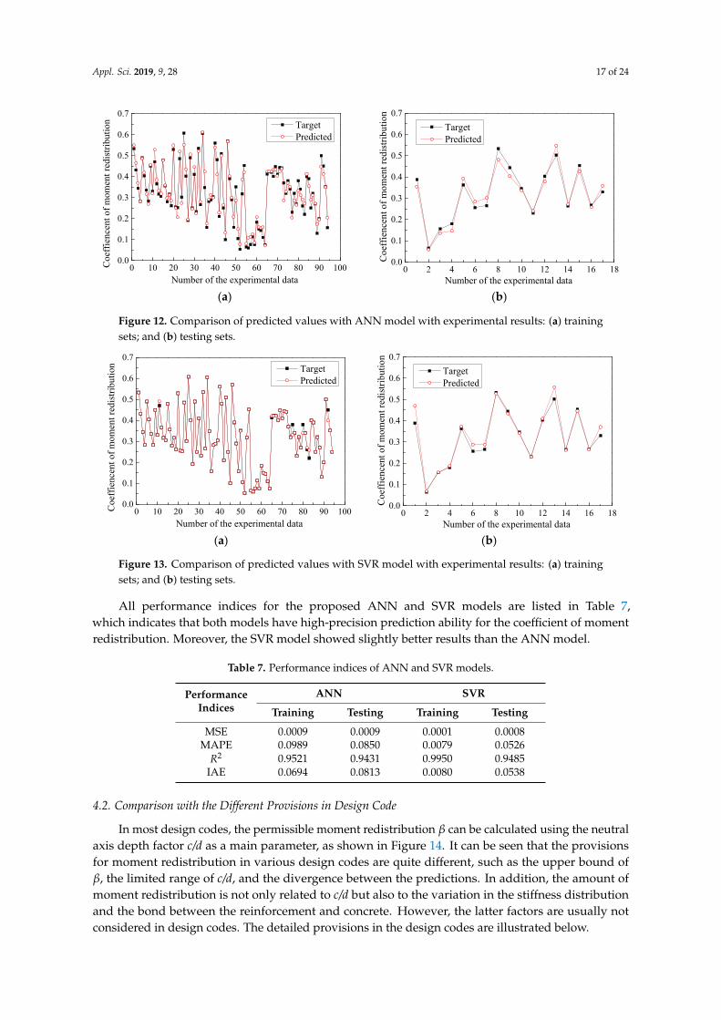
The ANN and SVR models developed in the present study were used to predict the coefficient ofmoment redistribution for statically indeterminate structures. The predicted values and experimentalresults of the two models for the training and testing sets are presented and compared in Figures 12and 13. It can be seen intuitively that the predicted values for the both models show good agreementwith the experimental values. To further evaluate the performance of the developed models,four indices of accuracy were calculated for the training and testing sets: mean squared error (MSE),determination coefficient (R2), mean absolute percentage error (MAPE) and integral absolute error(IAE). MSE and R2 are computed using Equations (3) and (4), respectively, and MAPE and IAE arecorrespondingly expressed as follows:

MAPE =1n

n

∑i=1

∣∣∣∣ ti − citi

∣∣∣∣ (13)

IAE =

n∑

i=1

[(ci − ti)

2]1/2

n∑

i=1ti

× 100% (14)

Appl. Sci. 2019, 9, 28 17 of 24



The ANN and SVR models developed in the present study were used to predict the coefficient of moment redistribution for statically indeterminate structures. The predicted values and experimental results of the two models for the training and testing sets are presented and compared in Figures 12 and 13. It can be seen intuitively that the predicted values for the both models show good agreement with the experimental values. To further evaluate the performance of the developed models, four indices of accuracy were calculated for the training and testing sets: mean squared error (MSE), determination coefficient (R2), mean absolute percentage error (MAPE) and integral absolute error (IAE). MSE and R2 are computed using Equations (3) and (4), respectively, and MAPE and IAE are correspondingly expressed as follows:

1

1MAPEn

i i

i i

t cn t=

−= (13)

1122

1

1

( )IAE 100%

n

i ii

n

ii

c t

t

=

=

− = ×

(14)

0 10 20 30 40 50 30 70 80 90 1000.0

0.1

0.2

0.3

0.4

0.5

0.3

0.7Co

effie

ncen

t of m

omen

t red

istrib

utio

n

Number of the experimental data

Target Predicted

0 2 4 3 8 10 12 14 13 18

0.0

0.1

0.2

0.3

0.4

0.5

0.3

0.7

Coef

fienc

ent o

f mom

ent r

edist

ribut

ion


Target Predicted

(a) (b)

Figure 12. Comparison of predicted values with ANN model with experimental results: (a) training sets; and (b) testing sets.

0 10 20 30 40 50 30 70 80 90 1000.0

0.1

0.2

0.3

0.4

0.5

0.3

0.7

Coef

fienc

ent o

f mom

ent r

edist

ribut

ion


Target Predicted

0 2 4 3 8 10 12 14 13 180.0

0.1

0.2

0.3

0.4

0.5

0.3

0.7Co

effie

ncen

t of m

omen

t red

istrib

utio

n


Target Predicted

(a) (b)

Figure 13. Comparison of predicted values with SVR model with experimental results: (a) training sets; and (b) testing sets.

Figure 12. Comparison of predicted values with ANN model with experimental results: (a) trainingsets; and (b) testing sets.



The ANN and SVR models developed in the present study were used to predict the coefficient of moment redistribution for statically indeterminate structures. The predicted values and experimental results of the two models for the training and testing sets are presented and compared in Figures 12 and 13. It can be seen intuitively that the predicted values for the both models show good agreement with the experimental values. To further evaluate the performance of the developed models, four indices of accuracy were calculated for the training and testing sets: mean squared error (MSE), determination coefficient (R2), mean absolute percentage error (MAPE) and integral absolute error (IAE). MSE and R2 are computed using Equations (3) and (4), respectively, and MAPE and IAE are correspondingly expressed as follows:

1

1MAPEn

i i

i i

t cn t=

−= (13)

1122

1

1

( )IAE 100%

n

i ii

n

ii

c t

t

=

=

− = ×

(14)

0 10 20 30 40 50 30 70 80 90 1000.0

0.1

0.2

0.3

0.4

0.5

0.3

0.7Co

effie

ncen

t of m

omen

t red

istrib

utio

n


Target Predicted

0 2 4 3 8 10 12 14 13 18

0.0

0.1

0.2

0.3

0.4

0.5

0.3

0.7

Coef

fienc

ent o

f mom

ent r

edist

ribut

ion


Target Predicted

(a) (b)

Figure 12. Comparison of predicted values with ANN model with experimental results: (a) training sets; and (b) testing sets.

0 10 20 30 40 50 30 70 80 90 1000.0

0.1

0.2

0.3

0.4

0.5

0.3

0.7

Coef

fienc

ent o

f mom

ent r

edist

ribut

ion


Target Predicted

0 2 4 3 8 10 12 14 13 180.0

0.1

0.2

0.3

0.4

0.5

0.3

0.7

Coef

fienc

ent o

f mom

ent r

edist

ribut

ion


Target Predicted

(a) (b)

Figure 13. Comparison of predicted values with SVR model with experimental results: (a) training sets; and (b) testing sets.

Figure 13. Comparison of predicted values with SVR model with experimental results: (a) trainingsets; and (b) testing sets.

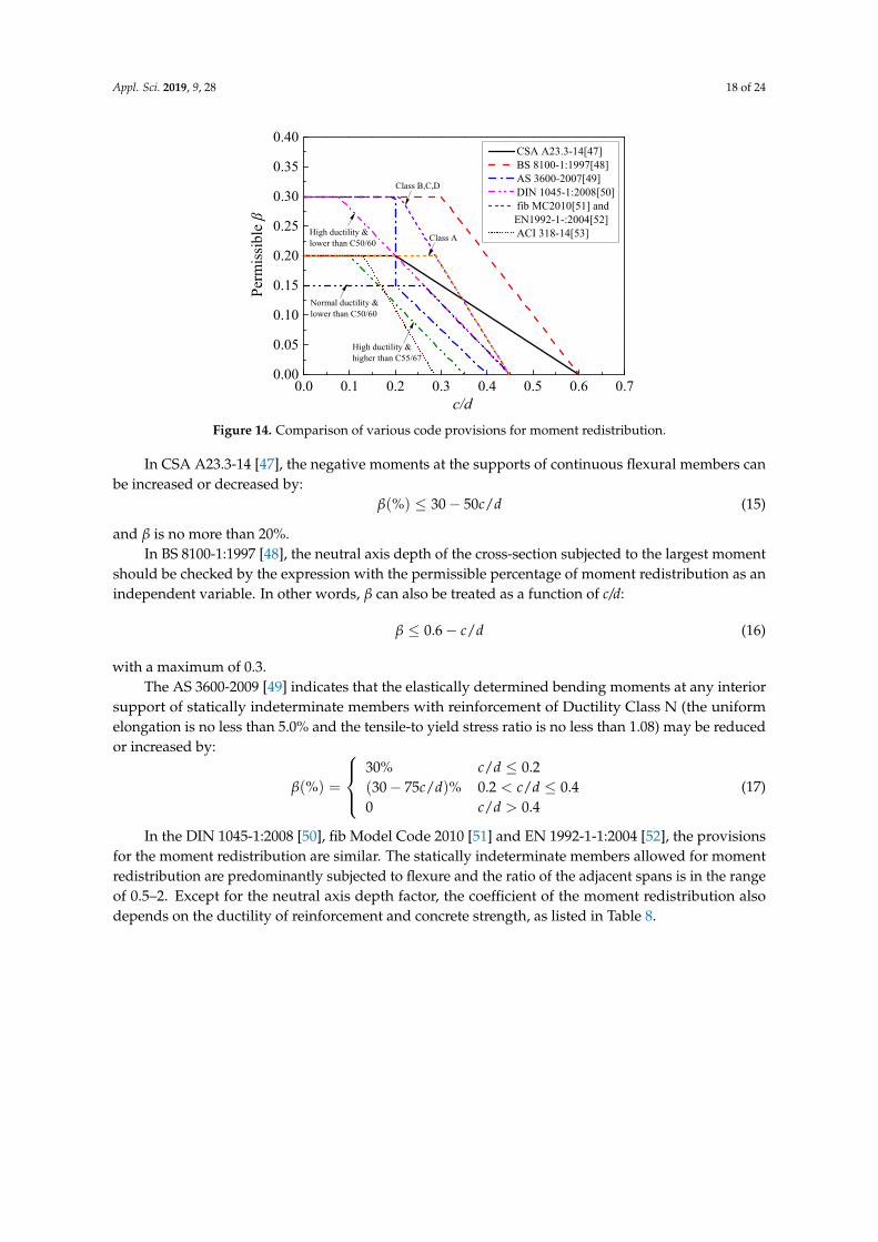
All performance indices for the proposed ANN and SVR models are listed in Table 7,which indicates that both models have high-precision prediction ability for the coefficient of momentredistribution. Moreover, the SVR model showed slightly better results than the ANN model.

Table 7. Performance indices of ANN and SVR models.

PerformanceIndices

ANN SVR

Training Testing Training Testing

MSE 0.0009 0.0009 0.0001 0.0008MAPE 0.0989 0.0850 0.0079 0.0526

R2 0.9521 0.9431 0.9950 0.9485IAE 0.0694 0.0813 0.0080 0.0538

4.2. Comparison with the Different Provisions in Design Code

In most design codes, the permissible moment redistribution β can be calculated using the neutralaxis depth factor c/d as a main parameter, as shown in Figure 14. It can be seen that the provisionsfor moment redistribution in various design codes are quite different, such as the upper bound ofβ, the limited range of c/d, and the divergence between the predictions. In addition, the amount ofmoment redistribution is not only related to c/d but also to the variation in the stiffness distributionand the bond between the reinforcement and concrete. However, the latter factors are usually notconsidered in design codes. The detailed provisions in the design codes are illustrated below.

Appl. Sci. 2019, 9, 28 18 of 24

0.0 0.1 0.2 0.3 0.4 0.5 0.6 0.70.00

0.05

0.10

0.15

0.20

0.25

0.30

0.35

0.40

Class A

Class B,C,D

Normal ductility &lower than C50/60

High ductility &higher than C55/67

CSA A23.3-14[47] BS 8100-1:1997[48] AS 3600-2007[49] DIN 1045-1:2008[50] fib MC2010[51] and

EN1992-1-:2004[52] ACI 318-14[53]

Perm

issib

le β

c/d

High ductility &lower than C50/60

Figure 14. Comparison of various code provisions for moment redistribution.

Figure 14. Comparison of various code provisions for moment redistribution.

In CSA A23.3-14 [47], the negative moments at the supports of continuous flexural members canbe increased or decreased by:

β(%) ≤ 30− 50c/d (15)

and β is no more than 20%.In BS 8100-1:1997 [48], the neutral axis depth of the cross-section subjected to the largest moment

should be checked by the expression with the permissible percentage of moment redistribution as anindependent variable. In other words, β can also be treated as a function of c/d:

β ≤ 0.6− c/d (16)

with a maximum of 0.3.The AS 3600-2009 [49] indicates that the elastically determined bending moments at any interior

support of statically indeterminate members with reinforcement of Ductility Class N (the uniformelongation is no less than 5.0% and the tensile-to yield stress ratio is no less than 1.08) may be reducedor increased by:

β(%) =

30% c/d ≤ 0.2(30− 75c/d)% 0.2 < c/d ≤ 0.40 c/d > 0.4

(17)

In the DIN 1045-1:2008 [50], fib Model Code 2010 [51] and EN 1992-1-1:2004 [52], the provisionsfor the moment redistribution are similar. The statically indeterminate members allowed for momentredistribution are predominantly subjected to flexure and the ratio of the adjacent spans is in the rangeof 0.5–2. Except for the neutral axis depth factor, the coefficient of the moment redistribution alsodepends on the ductility of reinforcement and concrete strength, as listed in Table 8.

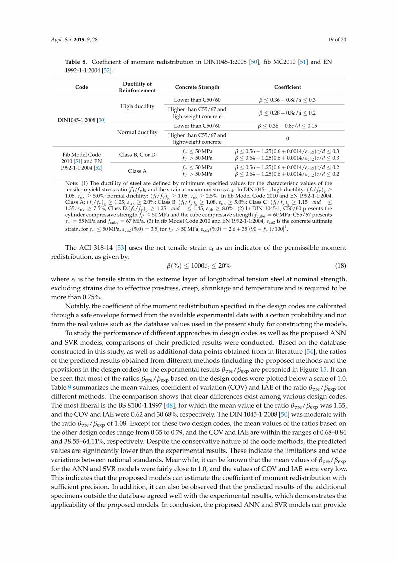
Appl. Sci. 2019, 9, 28 19 of 24

Table 8. Coefficient of moment redistribution in DIN1045-1:2008 [50], fib MC2010 [51] and EN1992-1-1:2004 [52].

Code Ductility ofReinforcement Concrete Strength Coefficient

DIN1045-1:2008 [50]

High ductilityLower than C50/60 β ≤ 0.36− 0.8c/d ≤ 0.3

Higher than C55/67 andlightweight concrete β ≤ 0.28− 0.8c/d ≤ 0.2

Normal ductilityLower than C50/60 β ≤ 0.36− 0.8c/d ≤ 0.15

Higher than C55/67 andlightweight concrete 0

Fib Model Code2010 [51] and EN1992-1-1:2004 [52]

Class B, C or Dfc′ ≤ 50 MPa β ≤ 0.56− 1.25(0.6 + 0.0014/εcu2)c/d ≤ 0.3fc′ > 50 MPa β ≤ 0.64− 1.25(0.6 + 0.0014/εcu2)c/d ≤ 0.3

Class Afc′ ≤ 50 MPa β ≤ 0.56− 1.25(0.6 + 0.0014/εcu2)c/d ≤ 0.2fc′ > 50 MPa β ≤ 0.64− 1.25(0.6 + 0.0014/εcu2)c/d ≤ 0.2

Note: (1) The ductility of steel are defined by minimum specified values for the characteristic values of thetensile-to-yield stress ratio (f t/f y)k and the strain at maximum stress εuk. In DIN1045-1, high ductility: ( ft/ fy)k ≥1.08, εuk ≥ 5.0%; normal ductility: ( ft/ fy)k ≥ 1.05, εuk ≥ 2.5%. In fib Model Code 2010 and EN 1992-1-1:2004,Class A: ( ft/ fy)k ≥ 1.05, εuk ≥ 2.0%; Class B: ( ft/ fy)k ≥ 1.08, εuk ≥ 5.0%; Class C: ( ft/ fy)k ≥ 1.15 and ≤1.35, εuk ≥ 7.5%; Class D:( ft/ fy)k ≥ 1.25 and ≤ 1.45, εuk ≥ 8.0%. (2) In DIN 1045-1, C50/60 presents thecylinder compressive strength fc′ ≤ 50 MPa and the cube compressive strength fcube = 60 MPa; C55/67 presentsfc′ = 55 MPa and fcube = 67 MPa. (3) In fib Model Code 2010 and EN 1992-1-1:2004, εcu2 is the concrete ultimatestrain, for fc′ ≤ 50 MPa, εcu2(%0) = 3.5; for fc′ > 50 MPa, εcu2(%0) = 2.6 + 35[(90− fc′ )/100]4.

The ACI 318-14 [53] uses the net tensile strain εt as an indicator of the permissible momentredistribution, as given by:

β(%) ≤ 1000εt ≤ 20% (18)

where εt is the tensile strain in the extreme layer of longitudinal tension steel at nominal strength,excluding strains due to effective prestress, creep, shrinkage and temperature and is required to bemore than 0.75%.

Notably, the coefficient of the moment redistribution specified in the design codes are calibratedthrough a safe envelope formed from the available experimental data with a certain probability and notfrom the real values such as the database values used in the present study for constructing the models.

To study the performance of different approaches in design codes as well as the proposed ANNand SVR models, comparisons of their predicted results were conducted. Based on the databaseconstructed in this study, as well as additional data points obtained from in literature [54], the ratiosof the predicted results obtained from different methods (including the proposed methods and theprovisions in the design codes) to the experimental results βpre/βexp are presented in Figure 15. It canbe seen that most of the ratios βpre/βexp based on the design codes were plotted below a scale of 1.0.Table 9 summarizes the mean values, coefficient of variation (COV) and IAE of the ratio βpre/βexp fordifferent methods. The comparison shows that clear differences exist among various design codes.The most liberal is the BS 8100-1:1997 [48], for which the mean value of the ratio βpre/βexp was 1.35,and the COV and IAE were 0.62 and 30.68%, respectively. The DIN 1045-1:2008 [50] was moderate withthe ratio βpre/βexp of 1.08. Except for these two design codes, the mean values of the ratios based onthe other design codes range from 0.35 to 0.79, and the COV and IAE are within the ranges of 0.68–0.84and 38.55–64.11%, respectively. Despite the conservative nature of the code methods, the predictedvalues are significantly lower than the experimental results. These indicate the limitations and widevariations between national standards. Meanwhile, it can be known that the mean values of βpre/βexp

for the ANN and SVR models were fairly close to 1.0, and the values of COV and IAE were very low.This indicates that the proposed models can estimate the coefficient of moment redistribution withsufficient precision. In addition, it can also be observed that the predicted results of the additionalspecimens outside the database agreed well with the experimental results, which demonstrates theapplicability of the proposed models. In conclusion, the proposed ANN and SVR models can provide

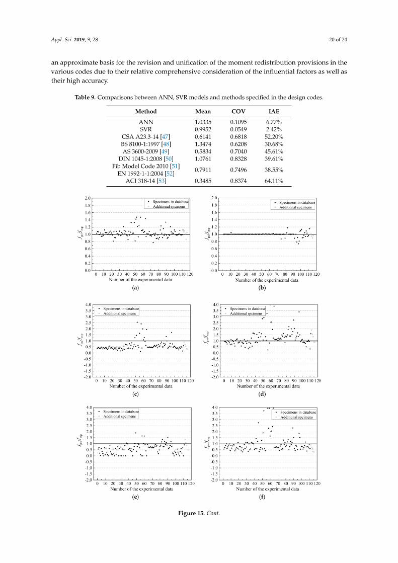
Appl. Sci. 2019, 9, 28 20 of 24

an approximate basis for the revision and unification of the moment redistribution provisions in thevarious codes due to their relative comprehensive consideration of the influential factors as well astheir high accuracy.

Table 9. Comparisons between ANN, SVR models and methods specified in the design codes.

Method Mean COV IAE

ANN 1.0335 0.1095 6.77%SVR 0.9952 0.0549 2.42%

CSA A23.3-14 [47] 0.6141 0.6818 52.20%BS 8100-1:1997 [48] 1.3474 0.6208 30.68%AS 3600-2009 [49] 0.5834 0.7040 45.61%

DIN 1045-1:2008 [50] 1.0761 0.8328 39.61%Fib Model Code 2010 [51]

EN 1992-1-1:2004 [52] 0.7911 0.7496 38.55%

ACI 318-14 [53] 0.3485 0.8374 64.11%

Figure 15. Cont.

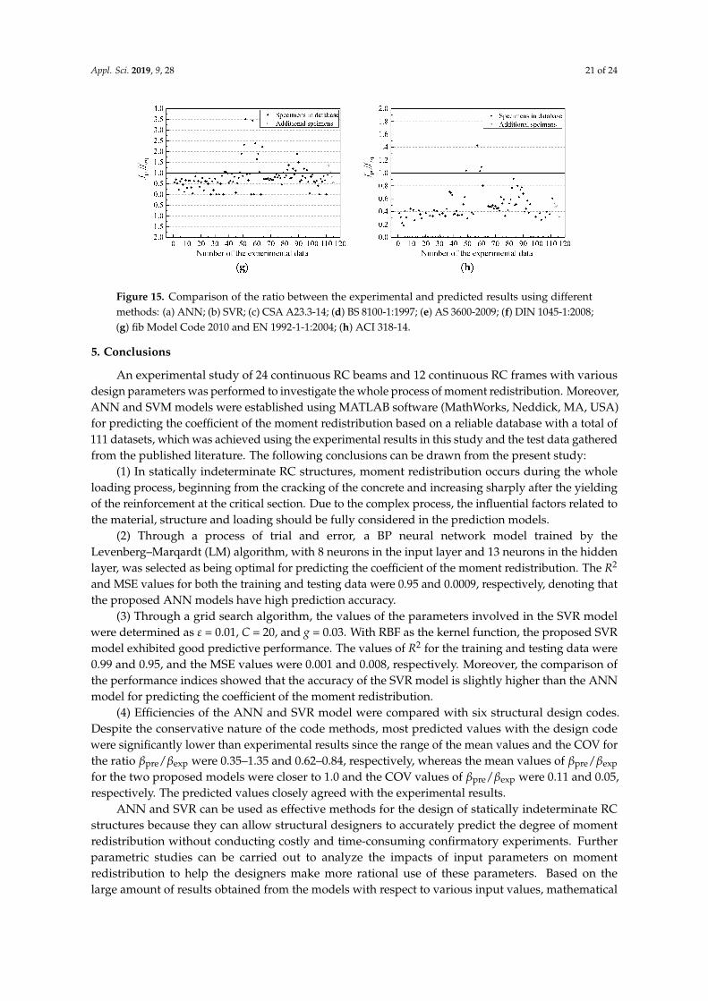
Appl. Sci. 2019, 9, 28 21 of 24

Figure 15. Comparison of the ratio between the experimental and predicted results using differentmethods: (a) ANN; (b) SVR; (c) CSA A23.3-14; (d) BS 8100-1:1997; (e) AS 3600-2009; (f) DIN 1045-1:2008;(g) fib Model Code 2010 and EN 1992-1-1:2004; (h) ACI 318-14.

5. Conclusions

An experimental study of 24 continuous RC beams and 12 continuous RC frames with variousdesign parameters was performed to investigate the whole process of moment redistribution. Moreover,ANN and SVM models were established using MATLAB software (MathWorks, Neddick, MA, USA)for predicting the coefficient of the moment redistribution based on a reliable database with a total of111 datasets, which was achieved using the experimental results in this study and the test data gatheredfrom the published literature. The following conclusions can be drawn from the present study:

(1) In statically indeterminate RC structures, moment redistribution occurs during the wholeloading process, beginning from the cracking of the concrete and increasing sharply after the yieldingof the reinforcement at the critical section. Due to the complex process, the influential factors related tothe material, structure and loading should be fully considered in the prediction models.

(2) Through a process of trial and error, a BP neural network model trained by theLevenberg–Marqardt (LM) algorithm, with 8 neurons in the input layer and 13 neurons in the hiddenlayer, was selected as being optimal for predicting the coefficient of the moment redistribution. The R2

and MSE values for both the training and testing data were 0.95 and 0.0009, respectively, denoting thatthe proposed ANN models have high prediction accuracy.

(3) Through a grid search algorithm, the values of the parameters involved in the SVR modelwere determined as ε = 0.01, C = 20, and g = 0.03. With RBF as the kernel function, the proposed SVRmodel exhibited good predictive performance. The values of R2 for the training and testing data were0.99 and 0.95, and the MSE values were 0.001 and 0.008, respectively. Moreover, the comparison ofthe performance indices showed that the accuracy of the SVR model is slightly higher than the ANNmodel for predicting the coefficient of the moment redistribution.

(4) Efficiencies of the ANN and SVR model were compared with six structural design codes.Despite the conservative nature of the code methods, most predicted values with the design codewere significantly lower than experimental results since the range of the mean values and the COV forthe ratio βpre/βexp were 0.35–1.35 and 0.62–0.84, respectively, whereas the mean values of βpre/βexp

for the two proposed models were closer to 1.0 and the COV values of βpre/βexp were 0.11 and 0.05,respectively. The predicted values closely agreed with the experimental results.

ANN and SVR can be used as effective methods for the design of statically indeterminate RCstructures because they can allow structural designers to accurately predict the degree of momentredistribution without conducting costly and time-consuming confirmatory experiments. Furtherparametric studies can be carried out to analyze the impacts of input parameters on momentredistribution to help the designers make more rational use of these parameters. Based on thelarge amount of results obtained from the models with respect to various input values, mathematical

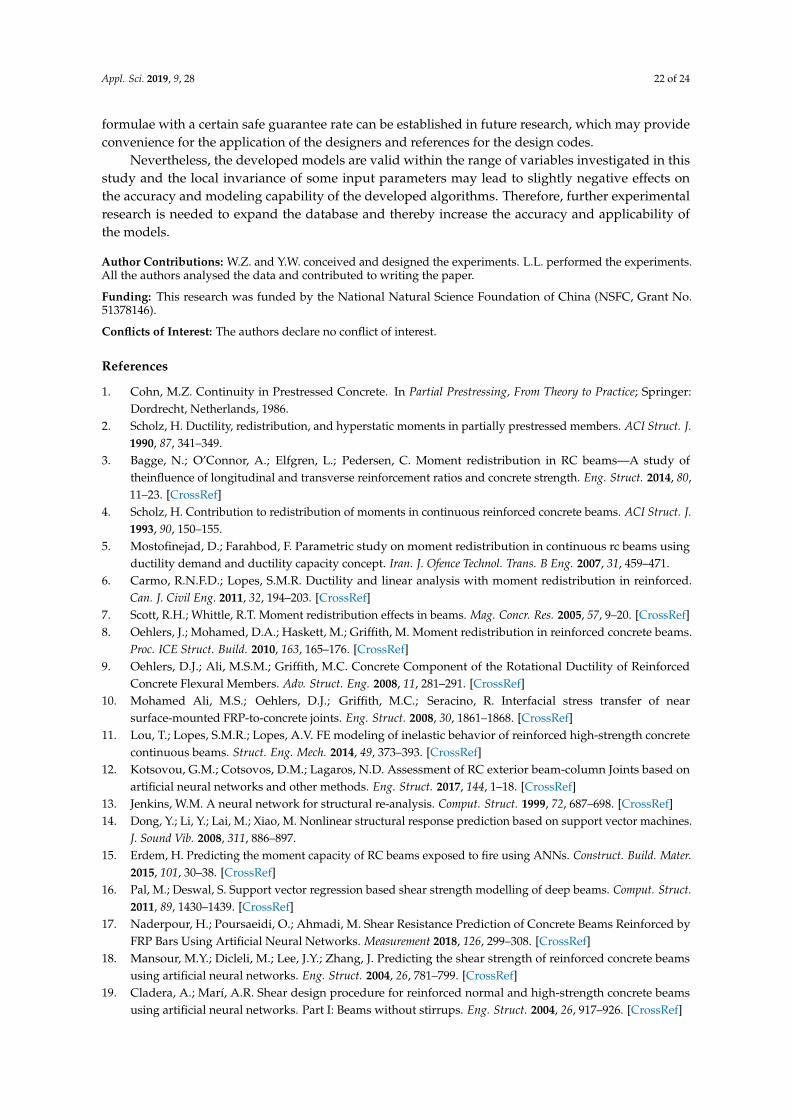
Appl. Sci. 2019, 9, 28 22 of 24

formulae with a certain safe guarantee rate can be established in future research, which may provideconvenience for the application of the designers and references for the design codes.

Nevertheless, the developed models are valid within the range of variables investigated in thisstudy and the local invariance of some input parameters may lead to slightly negative effects onthe accuracy and modeling capability of the developed algorithms. Therefore, further experimentalresearch is needed to expand the database and thereby increase the accuracy and applicability ofthe models.

Author Contributions: W.Z. and Y.W. conceived and designed the experiments. L.L. performed the experiments.All the authors analysed the data and contributed to writing the paper.

Funding: This research was funded by the National Natural Science Foundation of China (NSFC, Grant No.51378146).

Conflicts of Interest: The authors declare no conflict of interest.

References

1. Cohn, M.Z. Continuity in Prestressed Concrete. In Partial Prestressing, From Theory to Practice; Springer:Dordrecht, Netherlands, 1986.

2. Scholz, H. Ductility, redistribution, and hyperstatic moments in partially prestressed members. ACI Struct. J.1990, 87, 341–349.

3. Bagge, N.; O’Connor, A.; Elfgren, L.; Pedersen, C. Moment redistribution in RC beams—A study oftheinfluence of longitudinal and transverse reinforcement ratios and concrete strength. Eng. Struct. 2014, 80,11–23. [CrossRef]

4. Scholz, H. Contribution to redistribution of moments in continuous reinforced concrete beams. ACI Struct. J.1993, 90, 150–155.

5. Mostofinejad, D.; Farahbod, F. Parametric study on moment redistribution in continuous rc beams usingductility demand and ductility capacity concept. Iran. J. Ofence Technol. Trans. B Eng. 2007, 31, 459–471.

6. Carmo, R.N.F.D.; Lopes, S.M.R. Ductility and linear analysis with moment redistribution in reinforced.Can. J. Civil Eng. 2011, 32, 194–203. [CrossRef]

7. Scott, R.H.; Whittle, R.T. Moment redistribution effects in beams. Mag. Concr. Res. 2005, 57, 9–20. [CrossRef]8. Oehlers, J.; Mohamed, D.A.; Haskett, M.; Griffith, M. Moment redistribution in reinforced concrete beams.

Proc. ICE Struct. Build. 2010, 163, 165–176. [CrossRef]9. Oehlers, D.J.; Ali, M.S.M.; Griffith, M.C. Concrete Component of the Rotational Ductility of Reinforced

Concrete Flexural Members. Adv. Struct. Eng. 2008, 11, 281–291. [CrossRef]10. Mohamed Ali, M.S.; Oehlers, D.J.; Griffith, M.C.; Seracino, R. Interfacial stress transfer of near

surface-mounted FRP-to-concrete joints. Eng. Struct. 2008, 30, 1861–1868. [CrossRef]11. Lou, T.; Lopes, S.M.R.; Lopes, A.V. FE modeling of inelastic behavior of reinforced high-strength concrete

continuous beams. Struct. Eng. Mech. 2014, 49, 373–393. [CrossRef]12. Kotsovou, G.M.; Cotsovos, D.M.; Lagaros, N.D. Assessment of RC exterior beam-column Joints based on

artificial neural networks and other methods. Eng. Struct. 2017, 144, 1–18. [CrossRef]13. Jenkins, W.M. A neural network for structural re-analysis. Comput. Struct. 1999, 72, 687–698. [CrossRef]14. Dong, Y.; Li, Y.; Lai, M.; Xiao, M. Nonlinear structural response prediction based on support vector machines.

J. Sound Vib. 2008, 311, 886–897.15. Erdem, H. Predicting the moment capacity of RC beams exposed to fire using ANNs. Construct. Build. Mater.

2015, 101, 30–38. [CrossRef]16. Pal, M.; Deswal, S. Support vector regression based shear strength modelling of deep beams. Comput. Struct.

2011, 89, 1430–1439. [CrossRef]17. Naderpour, H.; Poursaeidi, O.; Ahmadi, M. Shear Resistance Prediction of Concrete Beams Reinforced by

FRP Bars Using Artificial Neural Networks. Measurement 2018, 126, 299–308. [CrossRef]18. Mansour, M.Y.; Dicleli, M.; Lee, J.Y.; Zhang, J. Predicting the shear strength of reinforced concrete beams

using artificial neural networks. Eng. Struct. 2004, 26, 781–799. [CrossRef]19. Cladera, A.; Marí, A.R. Shear design procedure for reinforced normal and high-strength concrete beams

using artificial neural networks. Part I: Beams without stirrups. Eng. Struct. 2004, 26, 917–926. [CrossRef]

http://dx.doi.org/10.1016/j.engstruct.2014.08.029

http://dx.doi.org/10.1139/l04-080

http://dx.doi.org/10.1680/macr.2005.57.1.9

http://dx.doi.org/10.1680/stbu.2010.163.3.165

http://dx.doi.org/10.1260/136943308785082571


http://dx.doi.org/10.12989/sem.2014.49.3.373


http://dx.doi.org/10.1016/S0045-7949(98)00311-3

http://dx.doi.org/10.1016/j.conbuildmat.2015.10.049

http://dx.doi.org/10.1016/j.compstruc.2011.03.005

http://dx.doi.org/10.1016/j.measurement.2018.05.051



Appl. Sci. 2019, 9, 28 23 of 24

20. Cascardi, A.; Micelli, F.; Aiello, M.A. An Artificial Neural Networks model for the prediction of thecompressive strength of FRP-confined concrete circular columns. Eng. Struct. 2017, 140, 199–208. [CrossRef]

21. Ahmadi, M.; Naderpour, H.; Kheyroddin, A. Utilization of artificial neural networks to prediction of thecapacity of CCFT short columns subject to short term axial load. Arch. Civil Mech. Eng. 2014, 14, 510–517.[CrossRef]

22. Kawashima, K.; Oreta, A.W.C. Neural Network Modeling of Confined Compressive Strength and Strain ofCircular Concrete Columns. J. Struct. Eng. 2003, 129, 554–561.

23. Tang, C.W.; Yen, T.; Chen, H.J. Modeling Confinement Efficiency of Reinforced Concrete Columns withRectilinear Transverse Steel Using Artificial Neural Networks. J. Struct. Eng. 2003, 129, 775–783. [CrossRef]

24. Khademi, F.; Akbari, M.; Nikoo, M. Displacement determination of concrete reinforcement building usingdata-driven models. Int. J. Sustain. Built Environ. 2017, 6, 400–411. [CrossRef]

25. Khademi, F.; Jamal, S.M.; Deshpande, N.; Londhe, S. Predicting strength of recycled aggregate concrete usingArtificial Neural Network, Adaptive Neuro-Fuzzy Inference System and Multiple Linear Regression. Int. J.Sustain. Built Environ. 2016, 5, 355–369. [CrossRef]

26. Sobhani, J.; Najimi, M.; Pourkhorshidi, A.R.; Parhizkar, T. Prediction of the compressive strength of no-slumpconcrete: A comparative study of regression, neural network and ANFIS models. Construct. Build. Mater.2010, 24, 709–718. [CrossRef]

27. Słonski, M. A comparison of model selection methods for compressive strength prediction ofhigh-performance concrete using neural networks. Comput. Struct. 2010, 88, 1248–1253. [CrossRef]

28. Tayfur, G.; Erdem, T.K.; Kırca, Ö. Strength Prediction of High-Strength Concrete by Fuzzy Logic and ArtificialNeural Networks. J. Mater. Civil Eng. 2014, 26, 04014079. [CrossRef]

29. Madandoust, R.; Bungey, J.H.; Ghavidel, R. Prediction of the concrete compressive strength by means ofcore testing using GMDH-type neural network and ANFIS models. Comput. Mater. Sci. 2012, 51, 261–272.[CrossRef]

30. Ince, R. Prediction of fracture parameters of concrete by Artificial Neural Networks. Eng. Fract. Mech. 2004,71, 2143–2159. [CrossRef]

31. Erdem, H. Prediction of the moment capacity of reinforced concrete slabs in fire using artificial neuralnetworks. Adv. Eng. Softw. 2010, 41, 270–276. [CrossRef]

32. Naser, M.Z. Deriving temperature-dependent material models for structural steel through artificialintelligence. Construct. Build. Mater. 2018, 191, 56–68. [CrossRef]

33. Meiyun, L. The Study of the Mechanical Property of HRB400 Reinforced Concrete Members; Zhengzhou University:Zhengzhou, China, 2003. (In Chinese)

34. Visintin, P.; Ali, M.S.M.; Xie, M.S.; Sturm, T. Experimental investigation of moment redistribution inultra-high performance fibre reinforced concrete beams. Construct. Build. Mater. 2018, 166, 433–444.[CrossRef]

35. Tao, J. The Static Experimental Study of the HRB500 Reinforced Concrete Frames; Hunan University: Changsha,China, 2009. (In Chinese)

36. Ting, Z. The Study of the Mechanical Property of HRB500 Reinforced Concrete Members; Zhengzhou University:Zhengzhou, China, 2004. (In Chinese)

37. Lin, C.-H.; Chien, Y.-M. Effect of section ductility on moment redistribution of continuous concrete beams.J. Chin. Inst. Eng. 2000, 23, 131–141. [CrossRef]

38. Code for Design of Concrete Structures GB 50010-2010; China Architecture and Building Press: Beijing, China,2011. (In Chinese)

39. Naderpour, H.; Kheyroddin, A.; Amiri, G.G. Prediction of FRP-confined compressive strength of concreteusing artificial neural networks. Compos. Struct. 2010, 92, 2817–2829. [CrossRef]

40. Rumerlhar, D.E. Learning representation by back-propagating errors. Nature 1986, 323, 533–536.41. Daliakopoulos, I.N.; Coulibaly, P.; Tsanis, I.K. Groundwater level forecasting using artificial neural networks.

J. Hydrol. 2005, 309, 229–240. [CrossRef]42. Boser, B.E.; Guyon, I.M.; Vapnik, V.N. A training algorithm for optimal margin classifiers. In Proceedings of

the Workshop on Computational Learning Theory, Pittsburgh, PA, USA, 27–29 July 1992; pp. 144–152.43. Behnood, A.; Verian, K.P.; Gharehveran, M.M. Evaluation of the splitting tensile strength in plain and steel

fiber-reinforced concrete based on the compressive strength. Construct. Build. Mater. 2015, 98, 519–529.[CrossRef]


http://dx.doi.org/10.1016/j.acme.2014.01.006

http://dx.doi.org/10.1061/(ASCE)0733-9445(2003)129:6(775)

http://dx.doi.org/10.1016/j.ijsbe.2017.07.002

http://dx.doi.org/10.1016/j.ijsbe.2016.09.003


http://dx.doi.org/10.1016/j.compstruc.2010.07.003

http://dx.doi.org/10.1061/(ASCE)MT.1943-5533.0000985

http://dx.doi.org/10.1016/j.commatsci.2011.07.053

http://dx.doi.org/10.1016/j.engfracmech.2003.12.004

http://dx.doi.org/10.1016/j.advengsoft.2009.07.006



http://dx.doi.org/10.1080/02533839.2000.9670531

http://dx.doi.org/10.1016/j.compstruct.2010.04.008

http://dx.doi.org/10.1016/j.jhydrol.2004.12.001


Appl. Sci. 2019, 9, 28 24 of 24

44. Vapnik, V.N. The Nature of Statistical Learning Theory; Springer: New York, NY, USA, 1995.45. Smola, A.; Burges, C.; Drucker, H.; Golowich, S.; Hemmen, L.V.; Muller, K.R.; Scholkopf, B.; Vapnik, V.

Regression Estimation with Support Vector Learning Machines. Master’s Thesis, Technische UniversitätMünchen, Munich, Germany, 2008.

46. Huang, Q.; Mao, J.; Liu, Y. An improved grid search algorithm of SVR parameters optimization.In Proceedings of the IEEE International Conference on Communication Technology, Chengdu, China,9–11 November 2012; pp. 1022–1026.

47. Canadian Standards Association. CSA A23.3-14: Design of Concrete Structures; Canadian StandardsAssociation: Toronto, ON, Canada, 2014.

48. British Standards Institution. BS8110: Structural Use OF Concrete Part 1:1997: Code of Practice for Design andConstruction; British Standards Institution: London, UK, 1997.

49. Australia Standards. AS 3600-2009: Concrete Structures; Australia Standards: Strathfield, Australia, 2009.50. German Institute of Standardisation (Deutesches Institut fur Normung). DIN 1045-3: Concrete Reinforced and

Prestressed Concrete Structures; DIN: Berlin, Germany, 2008.51. International Federation for Structural Concrete. FIB Model Code for Concrete Structures; International

Federation for Structural Concrete: Lausanne, Switzerland, 2010.52. British Standards Institution. EN 1992-1-1:2004 Eurocode 2: Design of Concrete Structures-Part 1-1: General

Rules and Rules for Buildings; British Standards Institution: London, UK, 2004.53. ACI Committee. American Concrete Institute and International Organization for Standardization, Building Code

Requirements for Structural Concrete (ACI318-14) and Commentary; American Concrete Institute: FarmingtonHills, MI, USA, 2014.

54. Li, L.; Zheng, W. Experimental study on plastic property of reactive power concrete continuous beams.J. Harbin Inst. Technol. 2010, 42, 193–199. (In Chinese)

© 2018 by the authors. Licensee MDPI, Basel, Switzerland. This article is an open accessarticle distributed under the terms and conditions of the Creative Commons Attribution(CC BY) license (http://creativecommons.org/licenses/by/4.0/).

http://creativecommons.org/

http://creativecommons.org/licenses/by/4.0/.

prediction of moment redistribution in statically

Documents