Purpose and expected outcomes

Most of the traits that plant breeders are interested in are quantitatively inherited. It is important to understandthe genetics that underlie the behavior of these traits in order to develop effective approaches for manipulating them.After studying this chapter, the student should be able to:

1 Define quantitative genetics and distinguish it from population genetics.2 Distinguish between qualitative traits and quantitative traits.3 Discuss polygenic inheritance.4 Discuss gene action.5 Discuss the variance components of quantitative traits.6 Discuss the concept of heritability of traits.7 Discuss selection and define the breeders’ equation.8 Discuss the concept of general worth of a plant.9 Discuss the concept of combining ability.

A quantitative geneticist observes the phenotype, a prod-uct of the genotype and the environment. The genotypicarray depends on mating systems and genetic linkagerelationships, as well as on allelic frequencies, which inturn are impacted by mutation, migration, random drift,and selection (see Chapter 7). To make effective obser-vations about phenotypes, the quantitative geneticisthas to make assumptions about the mating system,allelic frequency altering forces, and the environment.

Common assumptions of quantitative genetic analysisare as follow:

1 Reference population defined. Allelic and geno-typic frequencies can only be defined with respect to aspecified population. The researcher should define abase reference population. All inferences made aboutthe estimates should depend upon the compositionof this reference population.

8Introduction to

quantitative genetics

What is quantitative genetics?

Genetics has several branches, including populationgenetics, quantitative genetics, biometric genetics, andmolecular genetics. Population genetics is an extensionof Mendelian genetics applied at the population level.Population genetics does not assign a genotypic ornumerical value to each of the individuals (genotypes) inthe population (except in the case of coefficients ofselection). Quantitative genetics, on the other hand, isa branch of genetics in which individual genotypes areunidentified, and the traits of individuals are measured.Genotypic values are assigned to genotypes in the popu-lation. Quantitative genetics emphasizes the role ofselection in controlled populations of known ancestry.Some topics of population genetics are often discussedin quantitative genetics books, partly because popula-tion genetics is basic to quantitative genetics.

POPC08 28/8/06 4:08 PM Page 121

2 Absence of linkage. It is assumed that the trait (phenotype) observed is not affected by autosomallinkage genes.

3 Presence of diploid Mendelian inheritance. Theplants are assumed to be diploid in which genes segregate and assort independently. Analysis of polyploids is possible, but is involved and handleddifferently.

4 Absence of selection during the formation ofinbred lines. In order for the estimates of geneticvariances to pertain to the base reference population,it is required that no selection occur when inbredlines are crossed.

5 No breeding of the reference population. It isassumed that the inbreeding coefficient of the refer-ence population is zero. The analysis becomes morecomplex when inbreeding is coupled with more thantwo loci and includes the presence of epistasis.

Quantitative traits

The topic of quantitative traits was first discussed inChapter 5. Most traits encountered in plant breedingare quantitatively inherited. Many genes control suchtraits, each contributing a small effect to the overall phe-notypic expression of a trait. Variation in quantitativetrait expression is without natural discontinuities (i.e.,the variation is continuous). The traits that exhibit con-tinuous variations are also called metric traits. Anyattempt to classify such traits into distinct groups is onlyarbitrary. For example, height is a quantitative trait. Ifplants are grouped into tall versus short plants, onecould find relatively tall plants in the short group and,similarly, short plants in the tall group.

Qualitative genetics versus quantitative genetics

The major ways in which qualitative genetics and quan-titative genetics differ may be summarized as:

1 Nature of traits. Qualitative genetics is concernedwith traits that have Mendelian inheritance and can be described according to kind and, as previ-ously discussed, can be unambiguously categorized.Quantitative genetics traits are described in terms of the degree of expression of the trait, rather thanthe kind.

2 Scale of variability. Qualitative genetic traits providediscrete (discontinuous) phenotypic variation, whereasquantitative genetic traits produce phenotypic vari-ation that spans the full spectrum (continuous).

122 CHAPTER 8

3 Number of genes. In qualitative genetics, the effectsof single genes are readily detectable, while in quanti-tative genetics, single gene effects are not discernible.Rather, traits are under polygenic control (genes withsmall indistinguishable effects).

4 Mating pattern. Qualitative genetics is concernedwith individual matings and their progenies. Quan-titative genetics is concerned with a population ofindividuals that may comprise a diversity of matingkinds.

5 Statistical analysis. Qualitative genetic analysis isquite straightforward, and is based on counts andratios. On the other hand, quantitative analysis pro-vides estimates of population parameters (attributesof the population from which the sample wasobtained).

The environment and quantitative variation

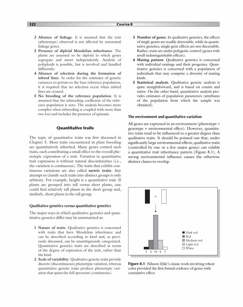
All genes are expressed in an environment (phenotype =genotype + environmental effect). However, quantita-tive traits tend to be influenced to a greater degree thanqualitative traits. It should be pointed out that, undersignificantly large environmental effects, qualitative traits(controlled by one or a few major genes) can exhibit a quantitative trait inheritance pattern (Figure 8.1). Astrong environmental influence causes the otherwisedistinct classes to overlap.

Figure 8.1 Nilsson-Ehle’s classic work involving wheatcolor provided the first formal evidence of genes withcumulative effect.

Dark redRedMedium redLight redWhite

16 4 141

×

POPC08 28/8/06 4:08 PM Page 122

Polygenes and polygenic inheritance

Quantitative traits are controlled by multiple genes orpolygenes.

What are polygenes?

Polygenes are genes with effects that are too small to beindividually distinguished. They are sometimes calledminor genes. In polygenic inheritance, segregationoccurs at a large number of loci affecting a trait. Thephenotypic expression of polygenic traits is susceptibleto significant modification by the variation in environ-mental factors to which plants in the population are subjected. Polygenic variation cannot be classified intodiscrete groups (i.e., variation is continuous). This isbecause of the large number of segregating loci, eachwith effects so small that it is not possible to identifyindividual gene effects in the segregating population orto meaningfully describe individual genotypes. Instead,biometrics is used to describe the population in terms of means and variances. Continuous variation is causedby environmental variation and genetic variation due tothe simultaneous segregation of many genes affectingthe trait. These effects convert the intrinsically discretevariation to a continuous one. Biometric genetics is usedto distinguish between the two factors that cause con-tinuous variability to occur.

Another aspect of polygenic inheritance is that differ-ent combinations of polygenes can produce a particularphenotypic expression. Furthermore, it is difficult tomeasure the role of the environment on trait expressionbecause it is very difficult to measure the environmentaleffect on the plant basis. Consequently, a breederattempting to breed a polygenic trait should evaluatethe cultivar in an environment that is similar to that prevailing in the production region. It is beneficial to plant breeding if a tight linkage of polygenes (called polygenic block or linkage block) that hasfavorable effects on traits of interest to the breeder is discovered.

In 1910, a Swedish geneticist, Nilsson-Ehle provideda classic demonstration of polygenic inheritance and in the process helped to bridge the gap between ourunderstanding of the essence of quantitative and quali-tative traits. Polygenic inheritance may be explained bymaking three basic assumptions:

1 Many genes determine the quantitative trait.2 These genes lack dominance.3 The action of the genes are additive.

Nilsson-Ehle crossed two varieties of wheat, one withdeep red grain of genotype R1R1R2R2, and the otherwhite grain of genotype r1r1r2r2. The results are sum-marized in Table 8.1. He observed that all the seed ofthe F1 was medium red. The F2 showed about 1/16dark red and 1/16 white seed, the remainder beingintermediate. The intermediates could be classified into6/16 medium red (like the F1), 4/16 red, and 4/16light red. The F2 distribution of phenotypes may beobtained as an expansion of the bionomial (a + b)4,where a = b = 1/2.

His interpretation was that the two genes each had apair of alleles that exhibited cumulative effects. In otherwords, the genes lacked dominance and their action wasadditive. Each R1 or R2 allele added some red to thephenotype so that the genotypes of white contained neither of these alleles, while the dark red genotype contained only R1 and R2. The phenotypic frequencyratio resulting from the F2 was 1 : 4 : 6 : 4 : 1 (i.e., 16genotypes and five classes) (see Figure 8.1).

The study involved only two loci. However, mostpolygenic traits are conditioned by genes at many loci.The number of genotypes that may be observed in theF2 is calculated as 3n, where n is the number of loci (eachwith two alleles). Hence, for three loci, the number ofgenotypes is 27, and for 10 loci, it will be 310 = 59,049.Many different genotypes can have the same phenotype,consequently, there is no strict one-to-one relationshipbetween genotypes (Table 8.2). For n genes, there are3n genotypes and 2n + 1 phenotypes. Many complextraits such as yield may have dozens and conceivablyeven hundreds of loci.

Other difficulties associated with studying the gen-etics of quantitative traits are dominance, environmentalvariation, and epistasis. Not only can dominanceobscure the true genotype, but both the amount anddirection can vary from one gene to another. For example, allele A may be dominant to a, but b may be

INTRODUCTION TO QUANTITATIVE GENETICS 123

Table 8.1 Transgressive segregation.

P1 R1R1R2R2 × r1r1r2r2(dark red) (white)

F1 R1r1R2r2

F2 1/16 = R1R1R2R24/16 = R1R1R2r2, R1r1R2R26/16 = R1R1r2r2, R1r1R2r2, r1r1R2R24/16 = R1r1r2r2, r1r1R2r21/16 = r1r1r2r2

POPC08 28/8/06 4:08 PM Page 123

dominant to B. It has previously been mentioned thatenvironmental effects can significantly obscure geneticeffects. Non-allelic interaction is a clear possibility whenmany genes are acting together.

Number of genes controlling a quantitative trait

Polygenic inheritance is characterized by segregation at a large number of loci affecting a trait as previouslydiscussed. Biometric procedures have been proposed toestimate the number of genes involved in a quantitativetrait expression. However, such estimates, apart fromnot being reliable, have limited practical use. Genes may differ in the magnitude of their effects on traits, notto mention the possibility of modifying gene effects oncertain genes.

Modifying genes

One gene may have a major effect on one trait, and aminor effect on another. There are many genes in plantswithout any known effects besides the fact that theymodify the expression of a major gene by either enhanc-ing or diminishing it. The effect of modifier genes maybe subtle, such as slight variations in traits like the shapeand shades of color of flowers, or, in fruits, variation in aroma and taste. Those trait modifications are of concern to plant breeders as they conduct breeding programs to improve quantitative traits involving manymajor traits of interest.

Decision-making in breeding based onbiometric genetics

Biometric genetics is concerned with the inheritance of quantitative traits. As previously stated, most of thegenes of interest to plant breeders are controlled by many

genes. In order to effectively manipulate quantitativetraits, the breeder needs to understand the nature andextent of their genetic and environmental control. M. J.Kearsey summarized the salient questions that need tobe answered by a breeder who is focusing on improvingquantitative (and also qualitative) traits, into four:

1 Is the character inherited?2 How much variation in the germplasm is genetic?3 What is the nature of the genetic variation?4 How is the genetic variation organized?

By having answers to these basic genetic questions, thebreeder will be in a position to apply the knowledge toaddress certain fundamental questions in plant breeding.

What is the best cultivar to breed?

As will be discussed later in the book, there are severaldistinct types of cultivars that plant breeders develop –pure lines, hybrids, synthetics, multilines, composites,etc. The type of cultivar is closely related to the breedingsystem of the species (self- or cross-pollinated), butmore importantly on the genetic control of the traits tar-geted for manipulation. As breeders have more under-standing of and control over plant reproduction, thetraditional grouping between types of cultivars to breedand the methods used along the lines of the breedingsystem have diminished. The fact is that the breedingsystem can be artificially altered (e.g., self-pollinatedspecies can be forced to outbreed, and vice versa).However, the genetic control of the trait of interest can-not be changed. The action and interaction of polygenesare difficult to alter. As Kearsey notes, breeders shouldmake decisions about the type of cultivar to breed based on the genetic architecture of the trait, especially thenature and extent of dominance and gene interaction,more so than the breeding system of the species.

Generally, where additive variance and additive ×additive interaction predominate, pure lines and inbredcultivars are appropriate to develop. However, wheredominance variance and dominance × dominance inter-action suggest overdominance predominates, hybridswould be successful cultivars. Open-pollinated cultivarsare suitable where a mixture of the above genetic archi-tectures occur.

What selection method would be most effective forimprovement of the trait?

The kinds of selection methods used in plant breedingare discussed in Chapters 16 and 17. The genetic control

124 CHAPTER 8

Table 8.2 As the number of genes controlling a traitincreases, the phenotypic classes become increasinglyindistinguishable. Given n genes, the number of possiblephenotypes in the F2 is given by 2n + 1.

Number of gene loci 1 2 3..................n

Ratio of F2 individuals expressing either extreme phenotype (parental) 1/4 1/16 1/64...........(1/4)n

POPC08 28/8/06 4:08 PM Page 124

of the trait of interest determines the most effectiveselection method to use. The breeder should pay atten-tion to the relative contribution of the components ofgenetic variance (additive, dominance, epistasis) andenvironmental variance in choosing the best selectionmethod. Additive genetic variance can be exploited forlong-term genetic gains by concentrating desirablegenes in the homozygous state in a genotype. Thebreeder can make rapid progress where heritability ishigh by using selection methods that are dependentsolely on phenotype (e.g., mass selection). However,where heritability is low, the method of selection basedon families and progeny testing are more effective and efficient. When overdominance predominates, thebreeder can exploit short-term genetic gain very quicklyby developing hybrid cultivars for the crop.

It should be pointed out that as self-fertilizing speciesattain homozygosity following a cross, they become lessresponsive to selection. However, additive genetic variancecan be exploited for a longer time in open-pollinatedpopulations because relatively more genetic variation is regularly being generated through the ongoing intermating.

Should selection be on single traits or multiple traits?

Plant breeders are often interested in more than onetrait in a breeding program, which they seek to improvesimultaneously. The breeder is not interested in achiev-ing disease resistance only, but in addition, high yieldand other agronomic traits. The problem with simultan-eous trait selection is that the traits could be correlatedsuch that modifying one affects the other. The conceptof correlated traits is discussed next. Biometric proced-ures have been developed to provide a statistical tool forthe breeder to use. These tools are also discussed in thissection.

Gene action

There are four types of gene action: additive, domin-ance, epistatic, and overdominance. Because geneeffects do not always fall into clear-cut categories, andquantitative traits are governed by genes with small indi-vidual effects, they are often described by their geneaction rather than by the number of genes by which theyare encoded. It should be pointed out that gene action isconceptually the same for major genes as well as minorgenes, the essential difference being that the action of a

minor gene is small and significantly influenced by theenvironment.

Additive gene action

The effect of a gene is said to be additive when eachadditional gene enhances the expression of the trait byequal increments. Consequently, if one gene adds oneunit to a trait, the effect of aabb = 0, Aabb = 1, AABb = 3,and AABB = 4. For a single locus (A, a) the heterozy-gote would be exactly intermediate between the parents(i.e., AA = 2, Aa = 1, aa = 0). That is, the performanceof an allele is the same irrespective of other alleles at the same locus. This means that the phenotype reflectsthe genotype in additive action, assuming the absence of environmental effect. Additive effects apply to theallelic relationship at the same locus. Furthermore, asuperior phenotype will breed true in the next genera-tion, making selection for the trait more effective toconduct. Selection is most effective for additive vari-ance; it can be fixed in plant breeding (i.e., develop acultivar that is homozygous).

Additive effect

Consider a gene with two alleles (A, a). Whenever Areplaces a, it adds a constant value to the genotype:

AA m Aa aabfffffffffffc*ffffffffffffg

bcdfgbcffffffffffgbcffffffffffg

+a –a

Replacing a by A in the genotype aa causes a change ofa units. When both aa are replaced, the genotype is 2aunits away from aa. The midparent value (the averagescore) between the two homozygous parents is given bym (representing a combined effect of both genes forwhich the parents have similar alleles and environmentalfactors). This also serves as the reference point for measuring deviations of genotypes. Consequently, AA = m + aA, aa = m − a, and Aa = m + dA, where aA isthe additive effect of allele A, and d is the dominanceeffect. This effect remains the same regardless of theallele with which it is combined.

Average effect

In a random mating population, the term average effectof alleles is used because there are no homozygous lines.Instead, alleles of one plant combine with alleles from

INTRODUCTION TO QUANTITATIVE GENETICS 125

POPC08 28/8/06 4:08 PM Page 125

pollen from a random mating source in the populationthrough hybridization to generate progenies. In effectthe allele of interest replaces its alternative form in anumber of randomly selected individuals in the popula-tion. The change in the population as a result of thisreplacement constitutes the average effect of the allele.In other words, the average effect of a gene is the meandeviation from the population mean of individuals thatreceived a gene from one parent, the gene from the otherparent having come at random from the population.

Breeding value

The average effects of genes of the parents determinethe mean genotypic value of the progeny. Further, thevalue of an individual judged by the mean value of itsprogeny is called the breeding value of the individual.This is the value that is transferred from an individual to its progeny. This is a measurable effect, unlike theaverage effect of a gene. However, the breeding valuemust always be with reference to the population towhich an individual is to be mated. From a practicalbreeding point of view, the additive gene effect is ofmost interest to breeders because its exploitation is pre-dictable, producing improvements that increase linearlywith the number of favorable alleles in the population.

Dominance gene action

Dominance action describes the relationship of alleles atthe same locus. Dominance variance has two compon-ents – variance due to homozygous alleles (which isadditive) and variance due to heterozygous genotypicvalues. Dominance effects are deviations from additivitythat make the heterozygote resemble one parent morethan the other. When dominance is complete, the het-erozygote is equal to the homozygote in effects (i.e., Aa = AA). The breeding implication is that the breedercannot distinguish between the heterozygous andhomozygous phenotypes. Consequently, both kinds ofplants will be selected, the homozygotes breeding truewhile the heterozygotes will not breed true in the nextgeneration (i.e., fixing superior genes will be less effec-tive with dominance gene action).

Dominance effect

Using the previous figure for additive effect, the extentof dominance (dA) is calculated as the deviation of the heterozygote, Aa, from the mean of the twohomozygotes (AA, aa). Also, dA = 0 when there is

no dominance while d is positive if A is dominant, and negative if aA is dominant. Further, if dominance is complete dA = aA, whereas dA < aA for incomplete (partial) dominance, and dA > aA for overdominace. Fora single locus, m = 1/2(AA + aa) and aA = 1/2(AA − aa),while dA = Aa − 1/2(AA + aa).

Overdominance gene action

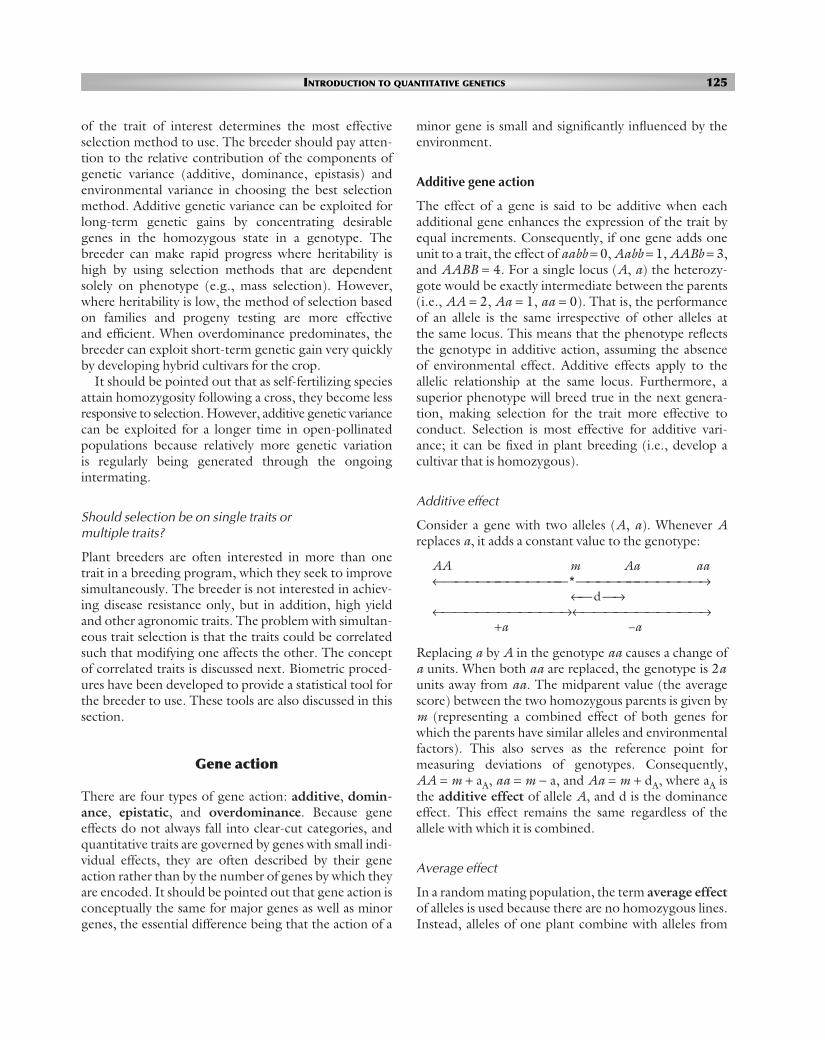
Overdominance gene action exists when each allele ata locus produces a separate effect on the phenotype, andtheir combined effect exceeds the independent effect ofthe alleles (i.e., aa = 1, AA = 1, Aa = 2) (Figure 8.2).From the breeding standpoint, the breeder can fix overdominance effects only in the first generation (i.e., F1 hybrid cultivars) through apomixis, or throughchromosome doubling of the product of a wide cross.

Epistasic gene action

Epistatic effects in qualitative traits are often describedas the masking of the expression of a gene by one atanother locus. In quantitative inheritance, epistasis isdescribed as non-allelic gene interaction. When twogenes interact, an effect can be produced where therewas none (e.g., Aabb = 0, aaBB = 0, but A–B– = 4).

The estimation of gene action or genetic variancerequires the use of large populations and a mating design.The effect of the environment on polygenes makes estimations more challenging. As N. W. Simmondsobserved, at the end of the day, what qualitative geneticanalysis allows the breeder to conclude from partition-ing variance in an experiment is to say that a portion ofthe variance behaves as though it could be attributed toadditive gene action or dominance effect, and so forth.

Variance components of a quantitative trait

The genetics of a quantitative trait centers on the studyof its variation. As D. S. Falconer stated, it is in terms of

126 CHAPTER 8

Figure 8.2 An illustration of overdominance gene action.The heterozygote, Aa, is more valuable than eitherhomozygote.

More like P1 More like P2

P1 P2Midparent

UnlikeP1 or P2

UnlikeP1 or P2

Phenotypicexpression

POPC08 28/8/06 4:08 PM Page 126

variation that the primary genetic questions are formu-lated. Further, the researcher is interested in partition-ing variance into its components that are attributed todifferent causes or sources. The genetic properties of apopulation are determined by the relative magnitudes ofthe components of variance. In addition, by knowing thecomponents of variance, one may estimate the relativeimportance of the various determinants of phenotype.

K. Mather expressed the phenotypic value of quanti-tative traits in this commonly used expression:

P (phenotype) = G (genotype) + E (environment)

Individuals differ in phenotypic value. When the pheno-types of a quantitative trait are measured, the observedvalue represents the phenotypic value of the individual.The phenotypic value is variable because it depends ongenetic differences among individuals, as well as environ-mental factors and the interaction between genotypesand the environment (called G × E interaction).

Total variance of a quantitative trait may be mathem-atically expressed as follows:

VP = VG + VE + VGE

where VP = total phenotypic variance of the segregatingpopulation, VG = genetic variance, VE = environmentalvariance, and VGE = variance associated with the geneticand environmental interaction.

The genetic component of variance may be furtherpartitioned into three components as follows:

VG = VA + VD + VI

where VA = additive variance (variance from additivegene effects), VD = dominance variance (variance fromdominance gene action), and VI = interaction (variancefrom interaction between genes). Additive genetic vari-ance (or simply additive variance) is the variance ofbreeding values and is the primary cause of resemblancebetween relatives. Hence VA is the primary determinantof the observable genetic properties of the population,and of the response of the population to selection.Further, VA is the only component that the researchercan most readily estimate from observations made onthe population. Consequently, it is common to partitiongenetic variance into two – additive versus all otherkinds of variance. This ratio, VA/VP, gives what is calledthe heritability of a trait, an estimate that is of practicalimportance in plant breeding (see next).

The total phenotypic variance may then be rewritten as:

VP = VA + VD + VI + VE + VGE

To estimate these variance components, the researcheruses carefully designed experiments and analytical methods. To obtain environmental variance, individualsfrom the same genotype are used.

An inbred line (essentially homozygous) consists ofindividuals with the same genotype. An F1 generationfrom a cross of two inbred lines will be heterozygous butgenetically uniform. The variance from the parents andthe F1 may be used as a measure of environmental vari-ance (VE). K. Mather provided procedures for obtaininggenotypic variance from F2 and backcross data. In sum,variances from additive, dominant, and environmentaleffects may be obtained as follows:

VP1 = E; VP2 = E; VF1 = EVF2 = 1/2A + 1/4D + EVB1 = 1/4A + 1/4D + EVB2 = 1/4A + 1/4D + EVB1 + VB2 = 1/2A + 1/2D + 2E

This represents the most basic procedure for obtainingcomponents of genetic variance since it omits the vari-ances due to epistasis, which are common with quantita-tive traits. More rigorous biometric procedures are neededto consider the effects of interlocular interaction.

It should be pointed out that additive variance anddominance variance are statistical abstractions ratherthan genetic estimates of these effects. Consequently,the concept of additive variance does not connote per-fect additivity of dominance or epistasis. To exclude thepresence of dominance or epistasis, all the genotypicvariance must be additive.

Concept of heritability

Genes are not expressed in a vacuum but in an environ-ment. A phenotype observed is an interaction betweenthe genes that encode it and the environment in whichthe genes are being expressed. Plant breeders typicallyselect plants based on the phenotype of the desired trait,according to the breeding objective. Sometimes, agenetically inferior plant may appear superior to otherplants only because it is located in a more favorableregion of the soil. This may mislead the breeder. Inother words, the selected phenotype will not give rise tothe same progeny. If the genetic variance is high and the

INTRODUCTION TO QUANTITATIVE GENETICS 127

POPC08 28/8/06 4:08 PM Page 127

environmental variance is low, the progeny will be likethe selected phenotype. The converse is also true. Ifsuch a plant is selected for advancing the breeding pro-gram, the expected genetic gain will not materialize.Quantitative traits are more difficult to select in a breeding program because they are influenced to agreater degree by the environment than are qualitat-ive traits. If two plants are selected randomly from amixed population, the observed difference in a specifictrait may be due to the average effects of genes (heredi-tary differences), or differences in the environments inwhich the plants grew up, or both. The average effectsof genes is what determines the degree of resemblancebetween relatives (parents and offspring), and hence iswhat is transmitted to the progenies of the selectedplants.

Definition

The concept of the reliability of the phenotypic value of a plant as a guide to the breeding value (additivegenotype) is called the heritability of the metric trait.As previously indicated, plant breeders are able to meas-ure phenotypic values directly, but it is the breedingvalue of individuals that determines their influence on the progeny. Heritability is the proportion of theobserved variation in a progeny that is inherited. Thebottom line is that if a plant breeder selects plants on the basis of phenotypic values to be used as parents in a cross, the success of such an action in changing thecharacteristics in a desired direction is predictable onlyby knowing the degree of correspondence (geneticdetermination) between phenotypic values and breed-ing values. Heritability measures this degree of corres-pondence. It does not measure genetic control, butrather how this control can vary.

Genetic determination is a matter of what causes a characteristic or trait; heritability, by contrast, is a scientific concept of what causes differences in a charac-teristic or trait. Heritability is, therefore, defined as afraction: it is the ratio of genetically caused variationto total variation (including both environmental andgenetic variation). Genetic determination, by contrast,is an informal and intuitive notion. It lacks quantitativedefinition, and depends on the idea of a normal environ-ment. A trait may be described as genetically determinedif it is coded in and caused by the genes, and bound todevelop in a normal environment. It makes sense to talkabout genetic determination in a single individual, butheritability makes sense only relative to a population inwhich individuals differ from one another.

Types of heritability

Heritability is a property of the trait, the population, andthe environment. Changing any of these factors willresult in a different estimate of heritability. There aretwo different estimates of heritability.

1 Broad sense heritability. Heritability estimated usingthe total genetic variance (VG) is called broad senseheritability. It is expressed mathematically as:

H = VG/VP

It tends to yield a high value (Table 8.3). Some usethe symbol H 2 instead of H.

2 Narrow sense heritability. Because the additivecomponent of genetic variance determines theresponse to selection, the narrow sense heritabilityestimate is more useful to plant breeders than thebroad sense estimate. It is estimated as:

h 2 = VA/VP

However, when breeding clonally propagated species(e.g., sugarcane, banana), in which both additive andnon-additive gene actions are fixed and transferredfrom parent to offspring, broad sense heritability isalso useful. The magnitude of narrow sense heritabil-ity cannot exceed, and is usually less than, the corres-ponding broad sense heritability estimate.

Heritabilities are seldom precise estimates because oflarge standard errors. Characters that are closely relatedto reproductive fitness tend to have low heritability estimates. The estimates are expressed as a fraction, but

128 CHAPTER 8

Table 8.3 Heritability estimates of some plantarchitectural traits in dry bean.

Trait Heritability

Plant height 45Hypocotyl diameter 38Number of branches/plant 56Nodes in lower third 36Nodes in mid section 45Nodes in upper third 46Pods in lower third 62Pods in mid section 85Pods in upper third 80Pod width 81Pod length 67Seed number per pod 30100 seed weight 77

POPC08 28/8/06 4:08 PM Page 128

may also be reported as a percentage by multiplying by100. A heritability estimate may be unity (1) or less.

Factors affecting heritability estimates

The magnitude of heritability estimates depends on thegenetic population used, the sample size, and the methodof estimation.

Genetic population

When heritability is defined as h2 = VA/VP (i.e., in thenarrow sense), the variances are those of individuals in the population. However, in plant breeding, certaintraits such as yield are usually measured on a plot basis(not on individual plants). The amount of genotypicvariance present for a trait in a population influencesestimates of heritability. Parents are responsible for the genetic structure of the populations they produce.More divergent parents yield a population that is moregenetically variable. Inbreeding tends to increase themagnitude of genetic variance among individuals in the population. This means that estimates derived fromF2 will differ from, say, those from F6.

Sample size

Because it is impractical to measure all individuals in alarge population, heritabilities are estimated from sam-ple data. To obtain the true genetic variance for a validestimate of the true heritability of the trait, the samplingshould be random. A weakness in heritability estimatesstems from bias and lack of statistical precision.

Method of computation

Heritabilities are estimated by several methods that use different genetic populations and produce estimatesthat may vary. Common methods include the variancecomponent method and parent–offspring regression.Mating schemes are carefully designed to enable thetotal genetic variance to be partitioned.

Methods of computation

The different methods of estimating heritabilities haveboth strengths and weaknesses.

Variance component method

The variance component method of estimating heri-tability uses the statistical procedure of analysis of

variance (ANOVA, see Chapter 9). Variance estimatesdepend on the types of populations in the experiment.Estimating genetic components suffers from certain statistical weaknesses. Variances are less accurately esti-mated than means. Also, variances are unrobost and sensitive to departure from normality. An example of aheritability estimate using F2 and backcross populationsis as follows:

VF2 = VA + VD + VEVB1 + VB2 = VA + 2VD + 2VEVE = VP1 + VP2 + VF1H = (VA + VD)/(VA + VD + VE) = VG/VPh2 = (VA)/(VA + VD + VE) = VA/VP

Example For example, using the data in the tablebelow:

P1 P2 F1 F2 BC1 BC2Mean 20.5 40.2 28.9 32.1 25.2 35.4Variance 10.1 13.2 7.0 52.3 35.1 56.5

VE = [VP1 + VP2 + VF1]/3= [10.1 + 13.2 + 7]/3= 30.3/3= 10.1

VA = 2VF2 − (VB1 + VB2)= 2(52.3) − (35.1 + 56.5)= 104.6 – 91.6= 13.0

VD = [(VB1 + VB2) − F2 − (VP1 + VP2 + F1)]/3= [(35.1 + 56.5) − 52.3 − (10.1 + 13.2 + 7.0)]/3= [91.6 − 52.3 − 30.3]/3= 3.0

Broad sense heritabilityH = [13.0 + 3.0]/[13.0 + 3.0 + 10.1]

= 16/26.1= 0.6130= 61.30%

Narrow sense heritabilityh2 = 13.0[13.0 + 3.0 + 10.1]

= 13.0/26.1= 0.4980= 49.80%

Other methods of estimationH = [VF2 − 1/2(VP1 + VP2)]/F2

= [52.3 − 1/2(10.1 + 13.2)]/52.3= 40.65/52.3= 0.7772= 77.72%

INTRODUCTION TO QUANTITATIVE GENETICS 129

POPC08 28/8/06 4:08 PM Page 129

This estimate is fairly close to that obtained by using theprevious formula.

Parent–offspring regression

The type of offspring determines if the estimate wouldbe broad sense or narrow sense. This method is based on several assumptions: the trait of interest has diploidMendelian inheritance; the population from which theparents originated is randomly mated; the population isin linkage equilibrium (or no linkage among loci con-trolling the trait); parents are non-inbred; and there isno environmental correlation between the performanceof parents and offspring.

The parent–offspring method of heritability is rela-tively straightforward. First, the parent and offspringmeans are obtained. Cross products of the paired valuesare used to compute the covariance. A regression of offspring on midparent value is then calculated.Heritability in the narrow sense is obtained as follows:

h2 = bop = VA/VP

where bop is the regression of offspring on midparentvalue, and VA and VP are the additive variance and phenotypic variance, respectively.

However, if only one parent is known or relevant(e.g., a polycross):

b = 1/2(VA/VP)

and

h2 = 2bop

Applications of heritability

Heritability estimates are useful for breeding quantita-tive traits. The major applications of heritability are:

1 To determine whether a trait would benefit frombreeding. If, in particular, the narrow sense heritabil-ity for a trait is high, it indicates that the use of plantbreeding methods will likely be successful in improv-ing the trait of interest.

2 To determine the most effective selection strategy touse in a breeding program. Breeding methods thatuse selection based on phenotype are effective whenheritability is high for the trait of interest.

3 To predict gain from selection. Response to selectiondepends on heritability. A high heritability would

likely result in high response to selection to advancethe population in the desired direction of change.

Evaluating parental germplasm

A useful application of heritability is in evaluating thegermplasm assembled for a breeding project to deter-mine if there is sufficient genetic variation for successfulimprovement to be pursued. A replicated trial of theavailable germplasm is conducted and analyzed byANOVA as follows:

Degrees of Error mean sumSource freedom (df) of squares (EMS)Replication r − 1Genotypes g − 1 σ2 + rσ2

gError (r − 1)(g − 1) σ2

From the analysis, heritability may be calculated as:

H/h2 = [σ2g]/[σ2

g + σ2e]

It should be pointed out that whether the estimate isheritability in the narrow or broad sense depends on the nature of the genotypes. Pure lines or inbred lineswould yield additive type of variance, making the esti-mate narrow sense. Segregating population would makethe estimate broad sense.

Response to selection in breeding

Selection was discussed in Chapter 7. The focus of thissection is on the response to selection (genetic gain orgenetic advance). After generating variability, the nexttask for the breeder is the critical one of advancing thepopulation through selection.

Selection, in essence, entails discriminating amonggenetic variation (heterogeneous population) to iden-tify and choose a number of individuals to establish thenext generation. The consequence of this is differentialreproduction of genotypes in the population such thatgene frequencies are altered, and, subsequently, thegenotypic and phenotypic values of the targeted traits.Even though artificial selection is essentially directional,the concept of “complete” or “pure” artificial selectionis an abstraction because, invariably, before the breedergets a chance to select plants of interest, some amount ofnatural selection has already been imposed.

The breeder hopes, by selecting from a mixed popula-tion, that superior individuals (with high genetic potential)

130 CHAPTER 8

POPC08 28/8/06 4:08 PM Page 130

will be advanced, and will consequently change the popu-lation mean of the trait in a positive way in the next generation. The breeder needs to have a clear objective.The trait to be improved needs to be clearly defined.Characters controlled by major genes are usually easy toselect. However, polygenic characters, being geneticallyand biologically complex, present a considerable chal-lenge to the breeder.

The response to selection (R) is the differencebetween the mean phenotypic value of the offspring ofthe selected parents and the whole of the parental gener-ation before selection. The response to selection is sim-ply the change of population mean between generationsfollowing selection. Similarly, the selection differential(S) is the mean phenotypic value of the individualsselected as parents expressed as a deviation from thepopulation mean (i.e., from the mean phenotypic valueof all the individuals in the parental generation beforeselection). Response to selection is related to heritabilityby the following equation:

R = h2S

Prediction of response in one generation: geneticadvance due to selection

The genetic advance achieved through selection dependson three factors:

1 The total variation (phenotypic) in the population inwhich selection will be conducted.

2 Heritability of the target character.3 The selection pressure to be imposed by the plant

breeder (i.e., the proportion of the population that isselected for the next generation).

A large phenotypic variance would provide the breederwith a wide range of variability from which to select.Even when the heritability of the trait of interest is veryhigh, genetic advance would be small without a largeamount of phenotypic variation (Figure 8.3). When theheritability is high, selecting and advancing only the top few performers is likely to produce a greater geneticadvance than selecting many moderate performers.However, such a high selection pressure would occur atthe expense of a rapid loss in variation. When heritabilityis low, the breeder should impose a lower selection pressure in order to advance as many high-potentialgenotypes as possible.

In principle, the prediction of response is valid foronly one generation of selection. This is so because a

response to selection depends on the heritability of thetrait estimated in the generation from which parents areselected. To predict the response in subsequent genera-tions, heritabilities must be determined in each genera-tion. Heritabilities are expected to change from onegeneration to the next because, if there is a response, itmust be accompanied by a change in gene frequencieson which heritability depends. Also, selection of parentsreduces the variance and the heritability, especially inthe early generations. It should be pointed out that heritability changes are not usually large.

If heritability is unity (VA = VP; no environmentalvariance), progress in a breeding program would be perfect, and the mean of the offspring would equal themean of the selected parents. On the other hand, if heri-tability is zero, there would be no progress at all (R = 0).

The response in one generation may be mathemati-cally expressed as:

X̄o − X̄p = R = ih2σ (or ∆G = ih2σp)

where X̄o = mean phenotype of the offspring of selectedparents, X̄p = mean phenotype of the whole parentalgeneration, R = advance in one generation of selection,h2 = heritability, σp = phenotypic standard deviation ofthe parental population, i = intensity of selection, and∆G = genetic gain or genetic advance.

This equation has been suggested by some to be one of the fundamental equations of plant breeding,which must be understood by all breeders, and hence is called the breeders’ equation. The equation is graphically illustrated in Figure 8.4. The factor “i”, the intensity of selection, is a statistical factor thatdepends on the fraction of the current populationretained to be used as parents for the next generation.The breeder may consult statistical tables for specific values (e.g., at 1% i = 2.668; at 5% i = 2.06; at 10% i = 1.755). The breeder must decide the selection intensity to achieve a desired objective. The selectiondifferential can be predicted if the phenotypic values of the trait of interest are normally distributed, and the selection is by truncation (i.e., the individuals areselected solely in order of merit according to their phenotypic value – no individual being selected is lessgood than any of those rejected).

The response equation is effective in predictingresponse to selection, provided the heritability estimate(h2) is fairly accurate. In terms of practical breeding, theparameters for the response equation are seldom avail-able and hence not widely used. Over the long haul,repeated selection tends to fix favorable genes, resulting

INTRODUCTION TO QUANTITATIVE GENETICS 131

POPC08 28/8/06 4:08 PM Page 131

in a decline in both heritability and phenotypic standarddeviation. Once genes have been fixed, there will be nofurther response to selection.

Example For example:

X σσp VP VA VEParents 15 2 6 4 3Offspring 20.2 15 4.3 2.5 3

R = ih2σp

Parentsh2 = VA/VP

= 4/6= 0.67

for i at P = 10% = 1.755 (read from tables and assuminga very large population).

R = 1.755 × 0.67 × 2= 2.35

Offspringh2 = VA/VP

= 2.5/4.3= 0.58

R = 1.755 × 0.58 × 1.5= 1.53

Generally, as selection advances to higher generations,genetic variance and heritability decline. Similarly, theadvance from one generation to the next declines, whilethe mean value of the trait being improved increases.

132 CHAPTER 8

Figure 8.3 The effect of phenotypic variance on genetic advance. (a) If the phenotypic variance is too small, the geneticvariability from which to select will be limited, resulting in a smaller genetic gain. (b) The reverse is true when thephenotypic variance is large.

0 5 10 15 20 25 30 35 40

Advance = 2.5

(a) (b)

0 5 10 15 20 25 30 35 40

Advance = 10

POPC08 28/8/06 4:08 PM Page 132

Concept of correlated response

Correlation is a measure of the degree of associationbetween traits as previously discussed. This associationmay be on the basis of genetics or may be non-genetic.In terms of response to selection, genetic correlation iswhat is useful. When it exists, selection for one trait willcause a corresponding change in other traits that arecorrelated. This response to change by genetic associ-ation is called correlated response. Correlated responsemay be caused by pleotropism or linkage disequilibrium.Pleotropism is the multiple effect of a single gene (i.e., asingle gene simultaneously affects several physiologicalpathways). In a random mating population, the role of linkage disequilibrium in correlated response is onlyimportant if the traits of interest are closely linked.

In calculating correlated response, genetic correla-tions should be used. However, the breeder often hasaccess to phenotypic correlation and can use them ifthey were estimated from values averaged over severalenvironments. Such data tend to be in agreement withgenetic correlation. In a breeding program the breeder,even while selecting simultaneously for multiple traits,

has a primary trait of interest and secondary traits. Thecorrelated response (CRy) to selection in the primarytrait (y) for a secondary trait (x) is given by:

CRy = ixhxhyρg√VPy

where hx and hy are square roots of the heritabilities ofthe two respective traits, and ρg is the genetic correlationbetween traits. This relationship may be reduced to:

CRy = ixρghx√VGy

since hy = √(VGy/VPy)It is clear that the effectiveness of indirect selection

depends on the magnitude of genetic correlation andthe heritability of the secondary traits being selected.Further, given the same selection intensity and a highgenetic correlation between the traits, indirect selectionfor the primary trait will be more effective than direc-tional selection, if heritability of the secondary trait ishigh (ρghx > hy). Such a scenario would occur when thesecondary trait is less sensitive to environmental change(or can be measured under controlled conditions). Also,when the secondary trait is easier and more economic to measure, the breeder may apply a higher selectionpressure to it.

Correlated response has wider breeding application in homozygous, self-fertilizing species and apomicts.Additive genetic correlation is important in selection inplant breeding. As previously discussed, the additivebreeding value is what is transferred to offspring and can be changed by selection. Hence, where traits areadditively genetically correlated, selection for one traitwill produce a correlated response in another.

Selection for multiple traits

Plant breeders may use one of three basic strategies tosimultaneously select multiple traits: tandem selection,independent curling, and selection index. Plantbreeders often handle very large numbers of plants in a segregating population using limited resources (time,space, labor, money, etc.). Along with the large numberof individuals are the many breeding characters oftenconsidered in a breeding program. The sooner they canreduce the numbers of plants to the barest minimum,but more importantly, to the most desirable and promis-ing individuals, the better. Highly heritable and readilyscorable traits are easier to select for in the initial stagesof a breeding program.

INTRODUCTION TO QUANTITATIVE GENETICS 133

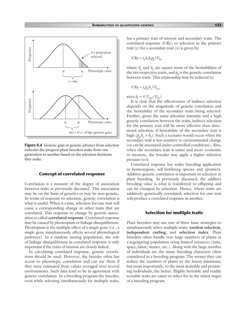
Figure 8.4 Genetic gain or genetic advance from selectionindicates the progress plant breeders make from onegeneration to another based on the selection decisionsthey make.

µsµ Phenotypic value

s = iσp

Freq

uenc

yFr

eque

ncy

b = proportionselected

µsµ Phenotypic value

∆G = h2s = ih2σp (genetic gain)

POPC08 28/8/06 4:08 PM Page 133

Tandem selection

In this mode of selection, the breeder focuses on onetrait at a time (serial improvement). One trait is selectedfor several generations, then another trait is focused on for the next period. The question of how long eachtrait is selected for before a switch and at what selec-tion intensity, are major considerations for the breeder.It is effective when genetic correlation does not existbetween the traits of interest, or when the relativeimportance of each trait changes throughout the years.

Independent curling

Also called truncation selection, independent curlingentails selecting for multiple traits in one generation.For example, for three traits, A, B, and C, the breedermay select 50% plants per family for A on phenotypicbasis, and from that group select 40% plants per familybased on trait B; finally, from that subset, 50% plants per family are selected for trait C, giving a total of 10%selection intensity (0.5 × 0.4 × 0.5).

Selection index

A breeder has a specific objective for conducting abreeding project. However, selection is seldom made onthe basis of one trait alone. For example, if the breedingproject is for disease resistance, the objective will be toselect a genotype that combines disease resistance withthe qualities of the elite adapted cultivar. Invariably,breeders usually practice selection on several traits,simultaneously. The problem with this approach is thatas more traits are selected for, the less the selection pres-sure that can be exerted on any one trait. Therefore, thebreeder should select on the basis of two or three traitsof the highest economic value. It is conceivable that atrait of high merit may be associated with other traits ofless economic value. Hence, using the concept of selec-tion on total merit, the breeder would make certaincompromises, selecting individuals that may not havebeen selected if the choice was based on a single trait.

In selecting on a multivariate phenotype, the breederexplicitly or implicitly assigns a weighting scheme to eachtrait, resulting in the creation of a univariate trait (anindex) that is then selected. The index is the best linearprediction of an individual’s breeding value. It takes theform of a multiple regression of breeding values on allthe sources of information available for the population.

The methods used for constructing an index usu-ally include heritability estimates, the relative economic

importance of each trait, and genetic and phenotypiccorrelation between the traits. The most common indexis a linear combination that is mathematically expressedas follows:

I = = bIz

where z = vector of phenotypic values in an individual,and b = vector of weights. For three traits, the form maybe:

I = aA1 + bB1 + cC1

where a, b, and c are coefficients correcting for relativeheritability and the relative economic importance oftraits A, B, and C, respectively, and A1, B1, and C1 arethe numerical values of traits A, B, and C expressed instandardized form. A standardized variable (X1) is cal-culated as:

X1 = (X − X̄ )/σx

where X = record of performance made by an individual,X̄ = average performance of the population, and σx =standard deviation of the trait.

The classic selection index has the following form:

I = b1x1 + b2x2 + b3x3 + . . . + bmxn

where x1, x2, x3, to xn are the phenotypic performance ofthe traits of interest, and b1, b2, and b3 are the relativeweights attached to the respective traits. The weightscould be simply the respective relative economic import-ance of each trait, with the resulting index called thebasic index, and may be used in cultivar assessment inofficial registration trials.

An index by itself is meaningless, unless it is used in comparing several individuals on a relative basis.Further, in comparing different traits, the breeder isfaced with the fact that the mean and variability of eachtrait is different, and frequently, the traits are measuredin different units. Standardization of variables resolvesthis problem.

Concept of intuitive index

Plant breeding was described in Chapter 2 as both a sci-ence and an art. Experience (with the crop, the methodsof breeding, breeding issues concerning the crop) isadvantageous in having success in solving plant breedingproblems. Plant breeders, as previously indicated, often

b zji

m

j=∑

1

134 CHAPTER 8

POPC08 28/8/06 4:08 PM Page 134

INTRODUCTION TO QUANTITATIVE GENETICS 135

Selection using a restricted index

Two commodities, protein meal and oil, are produced from soybean (Glycine max (L.) Merr.) and give the crop its value. Soybeanseeds are crushed, oil is extracted, and protein meal is what remains. On a dry weight basis, soybeans are approximately 20% oil and 40% protein. Concentration of protein in the meal is dependant on protein concentration in soybean seeds. Protein mealis traded either as 44% protein or 48% protein. The 48% protein meal is more valuable, so increasing or maintaining protein concentration in soybean seeds has been a breeding objective. Protein is negatively associated with oil in seeds and in manybreeding populations it is negatively associated with seed yield (Brim & Burton 1979).

The negative association between yield and protein could be due to genetic linkage as well as physiological processes (Carteret al. 1982). Thus a breeding strategy is needed that permits simultaneous selection of both protein and yield. Increased geneticrecombination should also be helpful in breaking unfavorable linkages between genes that contribute to the negative yield andprotein relation. We devised a recurrent S1 family selection program to satisfy the second objective and applied a restricted indexto family performance to achieve the first objective.

Selection procedure

A population designated RS4 was developed using both high-yielding and high protein parents. The high-yielding parents werethe cultivars, “Bragg”, “Ransom”, and “Davis”. The high protein parents were 10 F3 lines from cycle 7 of another recurrent selec-tion population designated IA (Brim & Burton 1979). In that population, selection had been solely for protein. Average proteinconcentration of the 10 parental F3 lines was 48.0%. The base or C0 population was developed by making seven or eight matings

between each high protein line and the threecultivars, resulting in 234 hybrids (Figure 1).The S0 generation was advanced at the USDepartment of Agriculture (USDA) winter soy-bean nursery in Puerto Rico resulting in 234 S1families. These were tested in two replicationsat two locations. Both seed yield and proteinconcentration were determined for each fam-ily. Average protein concentration of the ini-tial population was 45.6%. As this was anacceptable increase in protein, a restrictedselection index was applied aimed at increas-ing yield and holding protein constant. Thisindex was:

I = yield − (σGyp/σ2Gp) × protein

where σGyp = estimated genetic covariancebetween yield and protein, and σ2

Gp = estim-ated genetic variance of protein (Holbrook et al. 1989). Using this index, 29 families wereselected.

The following summer, these 29 families(now in the S2 generation) were randomlyintermated. To do this, we used the followingprocedure. Each day of the week, flowers forpollen were collected from 24 of the familiesand used to pollinate the remaining five famil-ies. A different set of 24 and five families wereused as males and females, respectively, each

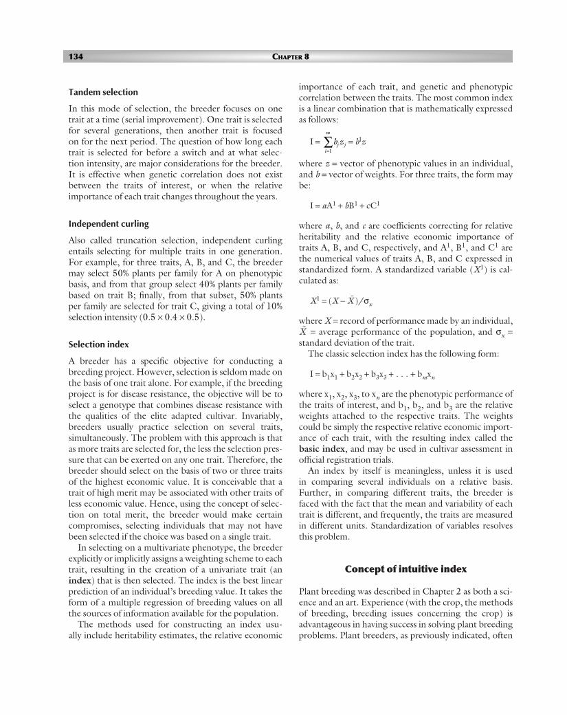
Figure 1 Recurrent S1 family selection for yield and seed proteinconcentration using a restricted index.

Year 1 Summer

Year 2 Summer

Year 3 Summer

Winter

10 high protein lines × 3 commercial cultivars

234 S0 plants

Self

234 S1 families

Yield test at two locations

Apply restricted indexSelect 29 families

Intermate S2 generation

Begin a new cycle

Modifiedpedigreeselection

Derive F6 linesEvaluate yield and seed composition

Cultivar selection

Industry highlightsRecurrent selection with soybean

Joe W. Burton

USDA Plant Science Building, 3127 Ligon Street, Raleigh, NC 27607, USA

POPC08 28/8/06 4:08 PM Page 135

136 CHAPTER 8

day. This process was followed until each family had at least seven successful pollinations on seven different plants within eachfamily. These were advanced in the winter nursery to generate the S1 families for the next cycle of selection.

Development of “Prolina” soybean

Modified pedigree selection was applied to the S1 families chosen in the first restricted index selection cycle. F6 lines were testedin replicated yield tests. One of those lines, N87-984, had good yielding ability and 45% seed protein concentration. Because ofheterogeneity for plant height within the line, F9 lines were derived from N87-984 using single-seed descent. These were yieldtested in multiple North Carolina locations. The two lines most desirable in terms of uniformity, protein concentration, and seedyield, were bulked for further testing and eventual release as the cultivar “Prolina” (Burton et al. 1999). At its release, “Prolina”had 45% protein compared with 42.7% for the check cultivar, “Centennial”, and similar yielding ability.

Recurrent selection using male sterility

In the previous example, intermating the selections was done using hand pollinations. Hand pollination with soybean is time-consuming and difficult. The average success rate in our program during the August pollinating season has been 35%. Thus, a

more efficient method for recom-bination would be helpful in a recur-rent selection program that dependson good random mating amongselected progeny for genetic recom-bination and reselection.

Genetic (nuclear) male sterility hasbeen used for this purpose. Severalnuclear male-sterile alleles have beenidentified (Palmer et al. 2004). Thefirst male-sterile allele to be discovered(ms1) is completely recessive (Brim &Young 1971) to the male-fertilityallele (Ms1). Brim and Stuber (1973)described ways that it could be usedin recurrent selection programs. Plantsthat are homozygous for the ms1 alleleare completely male-sterile. All seedsproduced on male-sterile plants resultfrom pollen contributed by a male-fertile plant (Ms1Ms1 or Ms1ms1) viaan insect pollen vector. The ms1ms1male-sterile plants are also partiallyfemale-sterile, so that seed set onmale-sterile plants is low in number,averaging about 35 seeds per plant.In addition, most pods have only oneseed and that seed is larger (30–40%larger) than seeds that would developon a fertile plant with a similar geneticbackground. The ms1 allele is main-tained in a line that is 50% ms1ms1and 50% Ms1ms1. This line is plantedin an isolation block. One-half of thepollen from male-fertile plants car-ries the Ms1 fertile allele and one-halfcarries the ms1 sterile allele. Male-sterile plants are pollinated by insectvectors, usually various bee species.At maturity, only seeds of male-sterileplants are harvested. These occur in the expected genotypic ratio of1/2Ms1ms1 : 1/2ms1ms1.

Figure 2 Recurrent mass selection for seed size in soybean using nuclear malesterility to intermate selections.

Year 1 Summer

Year 2 Summer

Winter

Fall

Planting: plant in a field isolation block. Space theplants 25–50 cm apart to permit larger plant growth

Random mating: when the plants flower, insect pollenvectors transfer pollen from flowers of male-fertile(Ms1–) to flowers of male-sterile (ms1ms1) plants

Seed harvest: when pods are mature on male-sterile plants,harvest 10–20 pods from 200 plants. Pick plants using somesystem (such as a grid) so that plants are sampled from allportions of the block

Selection: determine the seed size (average weight per seed)for each of the 200 plants. Select the 20 plants that have thelargest seeds

Intermate selections :bulk equal numbers of seedsfrom each of the 20 winternursery rows. Plant in an isolationblock for random mating

The next cycle begins

N79-1500A genetically diverse population that segregates for ms1 male sterility

Seed increase: grow the 20 selections in 20 separate rows in awinter nursery. At maturity, harvest fertile plants from each row

Bulk-self selections :grow remnant winternursery seeds of 20selected lines

Inbreed by bulk selfingor single-seed descent

Pure lines that are male-fertile (Ms1Ms1) can bederived in the F4 or latergeneration for furtherevaluation

POPC08 28/8/06 4:08 PM Page 136

INTRODUCTION TO QUANTITATIVE GENETICS 137

One of the phenotypic consequences of ms1 male sterility and low seed set is incomplete senescence. At maturity, soybeansnormally turn yellow, leaves abscise, and the pods and seeds dry. Seed and pods on male-sterile plants mature and dry normally,but the plants remain green and leaves do not abscise. Thus, they are easily distinguished from male-fertile plants.

To use nuclear male sterility in a recurrent selection experiment, a population is developed for improvement that segregates forone of the recessive male-sterile alleles. This can be accomplished in a number of ways depending on breeding objectives.Usually, a group of parents with desirable genes are mated to male-sterile genotypes. This can be followed by one or more back-crosses. Eventually, an F2 generation that segregates for male sterility is allowed to randomly intermate. Seeds are harvested frommale-sterile plants. Then several different selection units are possible. These include the male-sterile plant itself (Tinius et al.1991); the seeds (plants) from a single male-sterile plant (a half-sib family) (Burton & Carver 1993); and selfed seeds (plants) of anindividual from a male-sterile plant (S1 family) (Burton et al. 1990). Selection can be among and/or within the families (Carver et al.1986). If appropriate markers are employed, half-sib selection using a tester is also possible (Feng et al. 2004). As with all recurrentselection schemes, selected individuals are intermated. These can be either remnant seed of the selection unit or progeny of theselection unit. The male-sterile alleles segregate in both because both were derived in some manner from a single male-sterile plant.

Recurrent mass selection for seed size

Because seed set on male-sterile plants is generally low in number, we hypothesized that size of the seed was not limited bysource (photosynthate) inputs. Thus selecting male-sterile plants with the largest seeds would be selecting plants with the mostgenetic potential for producing large seeds. If so, this would mean that male-fertile plants derived from those selections wouldalso produce larger seeds and perhaps have increased potential for overall seed yield.

To test this hypothesis, we conducted recurrent mass selection for seed size (mg/seed) in a population, N80-1500, that segreg-ated for the ms1 male-sterile allele and had been derived from adapted high-yielding cultivar and breeding lines (Burton & Brim1981). The population was planted in an isolation block. Intermating between male-sterile and male-fertile plants occurred atrandom. In North Carolina there are numerous wild insect pollen vectors so introduction of domestic bees was not needed. Ifneeded, bee hives can be placed in or near the isolation block. At maturity, seeds were harvested from approximately 200 male-sterile plants. To make sure that the entire population was sampled, the block was divided into sections, and equal numbers ofplants were sampled from each section. Seeds from each plant were counted and weighed. The 20 plants with the largest seeds(greatest mass) were selected. These 20 selections were grown in a winter nursery and bulk-selfed to increase seed numbers.Equal numbers of seeds from the 20 selfed selections were combined and planted in another isolation block the following sum-mer to begin another selection cycle (Figure 2).

With this method, one cycle of selection is completed each year. This is mass selection where only the female parent isselected. Additionally the female parents all have an inbreeding coefficient of 0.5 because of the selfing seed increase during thewinter. Thus the expected genetic gain (∆G) for this selection scheme is:

∆G = S (0.75)σA2(σP

2)−1

where S = selection differential, σA2 = additive genetic variance, and σP

2 = phenotypic variance. This method was also used toincrease oleic acid concentration in seed lipids (Carver et al. 1986).

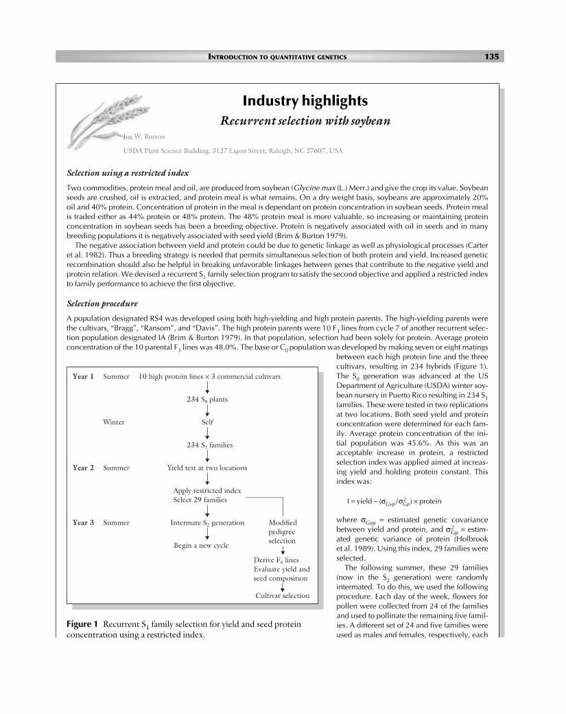
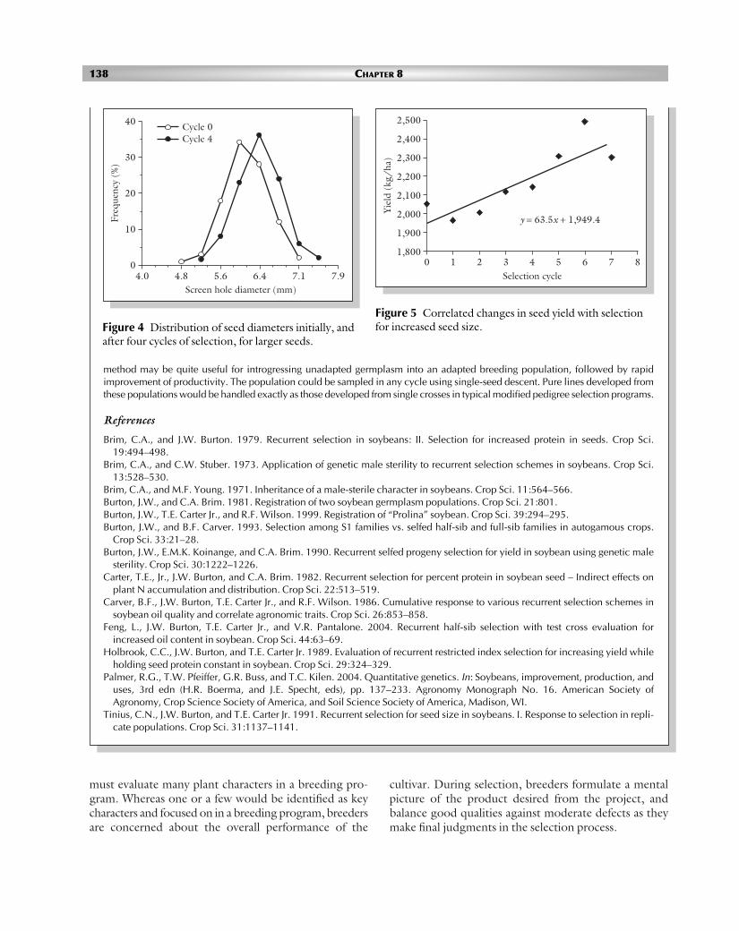
At the end of cycle 4 and cycle 7, selected materials fromeach cycle were evaluated in replicated field trials. Resultsof those trials showed that the method had successfullyincreased both seed size and yield in the population. Inseven cycles of selection, seed size of the male-sterile plantsincreased linearly from 182 to 235 mg/seed. Male-fertileseed size also increased linearly from 138 to 177 mg/seed(Figure 3). Not only the mass, but the physical size of theseeds increased. The range in seed diameter initially was4.8 to 7.1 mm. After four cycles of selection, the diameterrange had shifted and was 5.2 to 7.5 mm (Figure 4). Yieldincreased at an average rate of 63.5 kg/ha each cycle(Figure 5) or about 15% overall. There was some indicationthat after cycle 5 changes in yield were leveling off as yieldsof selections from cycle 5 and cycle 7 were very similar.

This method is relatively inexpensive. Little field space isrequired, and only a balance is needed to determine whichindividual should be selected. The ability to complete onecycle each year also makes it efficient. The largest expense isprobably that needed to increase the seeds from selectedmale-sterile plants in a winter greenhouse or nursery. The

Figure 3 Seed size changes with each selection for male-sterile and male-fertile soybeans.

240

220

200

180

160

140

120

Selection cycle0 1 2 3 4 5 6 7 8

Male-sterileMale-fertile

y = 8.3x + 181.7

y = 5.5x + 136.3

Seed

siz

e (m

g/se

ed)

POPC08 28/8/06 4:08 PM Page 137

must evaluate many plant characters in a breeding pro-gram. Whereas one or a few would be identified as keycharacters and focused on in a breeding program, breedersare concerned about the overall performance of the

cultivar. During selection, breeders formulate a mentalpicture of the product desired from the project, and balance good qualities against moderate defects as theymake final judgments in the selection process.

138 CHAPTER 8

method may be quite useful for introgressing unadapted germplasm into an adapted breeding population, followed by rapidimprovement of productivity. The population could be sampled in any cycle using single-seed descent. Pure lines developed fromthese populations would be handled exactly as those developed from single crosses in typical modified pedigree selection programs.

References

Brim, C.A., and J.W. Burton. 1979. Recurrent selection in soybeans: II. Selection for increased protein in seeds. Crop Sci.19:494–498.

Brim, C.A., and C.W. Stuber. 1973. Application of genetic male sterility to recurrent selection schemes in soybeans. Crop Sci.13:528–530.

Brim, C.A., and M.F. Young. 1971. Inheritance of a male-sterile character in soybeans. Crop Sci. 11:564–566.Burton, J.W., and C.A. Brim. 1981. Registration of two soybean germplasm populations. Crop Sci. 21:801.Burton, J.W., T.E. Carter Jr., and R.F. Wilson. 1999. Registration of “Prolina” soybean. Crop Sci. 39:294–295.Burton, J.W., and B.F. Carver. 1993. Selection among S1 families vs. selfed half-sib and full-sib families in autogamous crops.

Crop Sci. 33:21–28.Burton, J.W., E.M.K. Koinange, and C.A. Brim. 1990. Recurrent selfed progeny selection for yield in soybean using genetic male

sterility. Crop Sci. 30:1222–1226.Carter, T.E., Jr., J.W. Burton, and C.A. Brim. 1982. Recurrent selection for percent protein in soybean seed – Indirect effects on

plant N accumulation and distribution. Crop Sci. 22:513–519.Carver, B.F., J.W. Burton, T.E. Carter Jr., and R.F. Wilson. 1986. Cumulative response to various recurrent selection schemes in

soybean oil quality and correlate agronomic traits. Crop Sci. 26:853–858.Feng, L., J.W. Burton, T.E. Carter Jr., and V.R. Pantalone. 2004. Recurrent half-sib selection with test cross evaluation for

increased oil content in soybean. Crop Sci. 44:63–69.Holbrook, C.C., J.W. Burton, and T.E. Carter Jr. 1989. Evaluation of recurrent restricted index selection for increasing yield while

holding seed protein constant in soybean. Crop Sci. 29:324–329.Palmer, R.G., T.W. Pfeiffer, G.R. Buss, and T.C. Kilen. 2004. Quantitative genetics. In: Soybeans, improvement, production, and

uses, 3rd edn (H.R. Boerma, and J.E. Specht, eds), pp. 137–233. Agronomy Monograph No. 16. American Society ofAgronomy, Crop Science Society of America, and Soil Science Society of America, Madison, WI.

Tinius, C.N., J.W. Burton, and T.E. Carter Jr. 1991. Recurrent selection for seed size in soybeans. I. Response to selection in repli-cate populations. Crop Sci. 31:1137–1141.

Figure 4 Distribution of seed diameters initially, andafter four cycles of selection, for larger seeds.

40

30

20

10

0

Screen hole diameter (mm)4.0 4.8 5.6 6.4 7.1 7.9

Cycle 0Cycle 4

Freq

uenc

y (%

)

Figure 5 Correlated changes in seed yield with selectionfor increased seed size.

2,500

2,400

2,300

2,200

2,100

2,000

1,900

1,800

Selection cycle0 1 2 3 4 5 6 7 8

y = 63.5x + 1,949.4

Yiel

d (k

g/ha

)

POPC08 28/8/06 4:08 PM Page 138

Explicit indices are laborious, requiring the breeder to commit to extensive record-keeping and statisticalanalysis. Most breeders use a combination of truncationselection and intuitive selection index in their programs.

Concept of general worth

For each crop, there are a number of characters, whichconsidered together, define the overall desirability of thecultivar from the combined perspectives of the producerand the consumer. These characters may range betweenabout a dozen to several dozens, depending on the crop,and constitute the primary pool of characters that thebreeder may target for improvement. These charactersdiffer in importance (economic and agronomic) as wellas ease with which they can be manipulated throughbreeding. Plant breeders typically target one or few ofthese traits for direct improvement in a breeding pro-gram. That is, the breeder draws up a working list ofcharacters to address the needs embodied in the statedobjectives. Yield of the economic product is almost uni-versally the top priority in a plant breeding program.Disease resistance is more of a local issue, since whatmay be economically important in one region may notbe important in another area. Even though a plantbreeder may focus on one or a few traits at a time, theultimate objective is the improvement of the totality of the key traits that impact the overall desirability orgeneral worth of the crop. In other words, breeders ultimately have a holistic approach to selection in abreeding program. The final judgments are made on abalanced view of the essential traits of the crop.

Nature of breeding characteristics and theirlevels of expression

Apart from relative importance, the traits the plantbreeder targets vary in other ways. Some are readily evaluated by visual examination (e.g., shape, color,size), whereas others require a laboratory assay (e.g., oilcontent) or mechanical measurement (e.g., fiber charac-teristics of cotton). Special provisions (e.g., greenhouse,isolation block) may be required in disease breeding,whereas yield evaluations are most reliable when con-ducted over seasons and locations in the field.

In addition to choosing the target traits, the breederwill have to decide on the level of expression of eachone, below which a plant material would be declaredworthless. The acceptability level of expression of a trait

may be narrowly defined (stringent selection) or broadlydefined (loose selection). In industrial crops (e.g., cot-ton), the product quality may be strictly defined (e.g., a certain specific gravity, optimum length). In disease-resistance breeding, there may not be a significantadvantage of selecting for extreme resistance over select-ing for less than complete resistance. On the other hand,in breeding nutritional quality, there may be legal guide-lines as to threshold expression for toxic substances.

Early generation testing

Early generation testing is a selection procedure inwhich the breeder initiates testing of genetically hetero-geneous lines or families in an earlier than normal genera-tion. In Chapter 17, recurrent selection with testers was used to evaluate materials in early generations. Amajor consideration of the breeder in selecting a partic-ular breeding method is to maximize genetic gain peryear. Testing early, if effective, helps to identify andselect potential cultivars from superior families in theearly phase of the breeding program. The early genera-tion selection method has been favorably comparedwith other methods such as pedigree selection, single-seed descent, and bulk breeding. The question of howearly the test is implemented often arises. Should it be inthe F1-, F2- or F3-derived families? Factors to consider indeciding on the generation in which selection is doneinclude the trait being improved, and the availability of off-season nurseries to use in producing additionalgenerations per year (in lieu of selecting early).

Concept of combining ability

Over the years, plant breeders have sought ways of facilitating plant breeding through the efficient selec-tion of parents for a cross, effective and efficient selec-tion within a segregating population, and prediction ofresponse to selection, among other needs. Quantitativeassessment of the role of genetics in plant breedingentails the use of statistical genetics approaches to esti-mate variances and to partition them into components,as previously discussed. Because variance estimates areneither robust nor accurate, the direct benefits of statis-tical genetics to the breeder have been limited.

In 1942, Sprague and Tatum proposed a method of evaluation of inbred lines to be used in corn hybridproduction that was free of the genetic assumptions that accompany variance estimates. Called combining

INTRODUCTION TO QUANTITATIVE GENETICS 139

POPC08 28/8/06 4:08 PM Page 139

ability, the procedure entails the evaluation of a set ofcrosses among selected parents to ascertain the extent towhich variances among crosses are attributable to statis-tically additive characteristics of the parents, and whatcould be considered the effect of residual interactions.Crossing each line with several other lines produces anadditional measure in the mean performance of each linein all crosses. This mean performance of a line, whenexpressed as a deviation from the mean of all crosses,gives what Sprague and Tatum called the general com-bining ability (GCA) of the lines.

The GCA is calculated as the average of all F1s havingthis particular line as one parent, the value beingexpressed as a deviation from the overall mean ofcrosses. Each cross has an expected value (the sum ofGCAs of its two parental lines). However, each crossmay deviate from the expected value to a greater orlesser extent, the deviation being the specific combin-ing ability (SCA) of the two lines in combination. Thedifferences of GCA are due to the additive and additive× additive interactions in the base population. The dif-ferences in SCA are attributable to non-additive geneticvariance. Further, the SCA is expected to increase invariance more rapidly as inbreeding in the populationreaches high levels. The GCA is the average perform-ance of a plant in a cross with different tester lines, while the SCA measures the performance of a plant in aspecific combination in comparison with other crosscombinations.

The mathematical representation of this relationshipfor each cross is:

XAB = X̄ + GA + GB + SAB

where X̄ is the general mean and GA and GB are the gen-eral combining ability estimates of the parents, and SABis the statistically unaccounted for residual or specificcombining ability. The types of interactions that can beobtained depend upon the mating scheme used to pro-duce the crosses, the most common being the diallelmating design (full or partial diallel).

Plant breeders may use a variety of methods for esti-mating combining abilities, including the polycross andtopcrossing methods. However, the diallel cross (eachline is mated with every other line) developd by B.Griffing in 1956 is perhaps the most commonly usedmethod. The GCA of each line is calculated as follows:

Gx = [Tx/(n − 2)] − [∑T/n(n − 2)]

where x represents a specific line. Using the data inTable 8.4, GA can be calculated as:

GA = [TA/(n − 2)] − [∑T/n(n − 2)]= [226/(10 − 2)] − [2,024/10(10 − 2)]= 28.25 − 25.3= 2.95

The others may be calculated as for line A. The next stepis to calculate the expected value of each cross. Usingthe cross CD as an example, the expected value is calcu-lated as:

E(XCD) = −4.18 + 5.33 + 22.49 = 23.64

The SCA is calculated as follows:

SCACD = 26 − 23.64= 2.36

140 CHAPTER 8

Table 8.4 Calculating general and specific combining abilities.

B C D E F G H I J Total GCA

A 26 24 29 28 22 21 27 21 28 226 2.98B 21 35 30 26 22 29 14 19 222 2.45C 26 21 10 14 13 17 23 169 –4.18D 25 31 32 28 21 18 245 5.33E 13 23 15 15 14 184 –2.3F 20 31 17 15 185 –2.18G 32 14 12 190 –1.55H 35 38 248 5.7I 17 171 –3.93J 184 –2.3

2,024 0

POPC08 28/8/06 4:08 PM Page 140

This is done for each combination and a plot ofobserved values versus expected values plotted. Becausethe values of SCA are subject to sampling error, thepoints on the plot do not lie on the diagonal. The dis-tance from each point to the diagonal represents theSCA plus sampling error of the cross. Additional errorwould occur if the lines used in the cross are not highlyinbred (error due to the sampling of genotypes from thelines).

Combining ability calculations are statistically robust,being based on first-degree statistics (totals, means). No genetic assumptions are made about individuals.The concept is applicable to both self-pollinated andcross-pollinated species, for identifying desirable crosscombinations of inbred lines to include in a hybrid program or for developing synthetic cultivars. It is usedto predict the performance of hybrid populations ofcross-pollinated species, usually via a testcross or poly-cross. It should be pointed out that combining abilitycalculations are properly applied only in the context inwhich they were calculated. This is because GCA valuesare relative and depend upon the mean of the chosenparent materials in the crosses.

A typical ANOVA for combining ability analysis is asfollows:

Sum of Mean sum squares of squares

Source df (SS) (MS) EMSGCA p − 1 SG MG σ2

E + σ2SCA + σ2

GCASCA p(p − 1)/2 SS MS σ2

E + σ2SCA

Error m SE ME σ2E

The method used for a combining ability analysisdepends on the available data:

1 Parents + F1 or F2 and reciprocal crosses (i.e., p2

combinations).2 Parents + F1 or F2, without reciprocals (i.e., 1/2p(p + 1)

combinations).3 F1 + F2 + reciprocals, without parents and reciprocals

(i.e., 1/2p(p − 1) combinations).4 Only F1 generations, without parents and reciprocals

(i.e., 1/2p(p − 1) combinations).

Mating designs

Artificial crossing or mating is a common activity inplant breeding programs for generating various levels of relatedness among the progenies that are produced.Mating in breeding has two primary purposes:

1 To generate information for the breeder to under-stand the genetic control or behavior of the trait ofinterest.

2 To generate a base population to initiate a breedingprogram.

The breeder influences the outcome of a mating by the choice of parents, the control over the frequencywith which each parent is involved in mating, and thenumber of offspring per mating, among other ways. Amating may be as simple as a cross between two parents,to the more complex diallel mating.

Hybrid crosses

These are reviewed here to give the student a basis forcomparison with the random mating schemes to be presented.

1 Single cross = A × B → F1 (AB)2 Three-way cross = (A × B) → F1 × C → (ABC)3 Backcross = (A × B) → F1 × A → (BC1)4 Double cross = (A × B) → FAB; (C × D) → FCD;

FAB × FCD → (ABCD)

These crosses are relatively easy to genetically analyze.The breeder exercises significant control over the mat-ing structure.

Mating designs for random mating populations

The term mating design is usually applied to schemesused by breeders and geneticists to impose random mat-ing for a specific purpose. To use these designs, certainassumptions are made by the breeder:

1 The materials in the population have diploid beha-vior. However, polyploids that can exhibit disomicinheritance (alloploids) can be studied.

2 The genes controlling the trait of interest are inde-pendently distributed among the parents (i.e., uncor-related gene distribution).

3 The absence of: non-allelic interactions, reciprocaldifferences, multiple alleles at the loci controlling thetrait, and G × E interactions.

Biparental mating (or paired crosses)

In this design, the breeder selects a large number ofplants (n) at random and crosses them in pairs to pro-duce 1/2n full-sib families. The biparental (BIP) is thesimplest of the mating designs. If r plants per progeny

INTRODUCTION TO QUANTITATIVE GENETICS 141

POPC08 28/8/06 4:08 PM Page 141

family are evaluated, the variation within (w) andbetween (b) families may be analyzed as follows:

Source df MS EMSBetween families (1/2n) − 1 MS1 σ2w + rσ2bWithin families 1/2n(r − 1) MS2 σ2w

where σ2b is the covariance of full sibs (σ2b = 1/2VA +1/4VD + VEC = 1/r (MS1 − MS2) and σ2w = 1/2VA + 3/4VD+ VEW = MS2.

The limitation of this otherwise simple to implementdesign is its inability to provide the needed informationto estimate all the parameters required by the model.The progeny from the design comprise full sibs or unre-lated individuals. There is no further relatedness amongindividuals in the progeny. The breeder must makeunjustifiable assumptions in order to estimate thegenetic and environmental variance.

Polycross

This design is for intermating a group of cultivars bynatural crossing in an isolated block. It is most suited tospecies that are obligate cross-pollinaters (e.g., foragegrasses and legumes, sugarcane, sweet potato), butespecially to those that can be vegetatively propagated.It provides an equal opportunity for each entry to becrossed with every other entry. It is critical that theentries be equally represented and randomly arranged inthe crossing block. If 10 or less genotypes are involved,the Latin square design may used. For a large number of entries, the completely randomized block design maybe used. In both cases, about 20–30 replications areincluded in the crossing block. The ideal requirementsare hard to meet in practice because of several problems,placing the system in jeopardy of deviating from randommating. If all the entries do not flower together, matingwill not be random. To avoid this, the breeder may plantlate flowering entries earlier.

Pollen may not be dispersed randomly, resulting inconcentrations of common pollen in the crossing block.Half sibs are generated in a polycross because progenyfrom each entry has a common parent. The design isused in breeding to produce synthetic cultivars, recom-bining selected entries of families in recurrent selectionbreeding programs, or for evaluating the GCA of entries.

North Carolina Design I

Design I is a very popular multipurpose design for boththeoretical and practical plant breeding applications

(Figure 8.5). It is commonly used to estimate additiveand dominance variances as well as for the evaluation of full- and half-sib recurrent selection. It requiressufficient seed for replicated evaluation trials, and henceis not of practical application in breeding species that arenot capable of producing large amounts of seed. It isapplicable to both self- and cross-pollinated species thatmeet this criterion. As a nested design, each member ofa group of parents used as males is mated to a differentgroup of parents. NC Design I is a hierarchical designwith non-common parents nested in common parents.

The total variance is partitioned as follows:

Source df MS EMSMales n − 1 MS1 σ2w + rσ2

mf + r fσ2m

Females n1(n2 − 1) MS2 σ2w + rσ2mf

Within progenies n1n2(r − 1) MS3 σ2w

σ2m = [MS1 − MS2]/rn2 = 1/4VA

rσ2mf = [MS2 − MS3]/r = 1/4VA + 1/4VD

σ2w = MS3 = 1/2VA + 3/4VD + E

This design is most widely used in animal studies. Inplants, it has been extensively used in maize breeding forestimating genetic variances.

North Carolina Design II

In this design, each member of a group of parents usedas males is mated to each member of another group of

142 CHAPTER 8

Figure 8.5 North Carolina Design I. (a) This design is anested arrangement of genotypes for crossing in which nomale is involved in more than one cross. (b) A practicallayout in the field.

A

A

D

ADD

AEE

AFF

B

BGG

BHH

BII

C

CJJ

CKK

CLLProgenyFemalesMales

(a) Conceptual (b) Practical (basic)

B C

E

F

G

H

I

J

K Female

L

Male

POPC08 28/8/06 4:08 PM Page 142

parents used as females. Design II is a factorial matingscheme similar to Design I (Figure 8.6). It is used toevaluate inbred lines for combining ability. The design ismost adapted to plants that have multiple flowers so thateach plant can be used repeatedly as both male andfemale. Blocking is used in this design to allow all themating involving a single group of males to a singlegroup of females to be kept intact as a unit. The design isessentially a two-way ANOVA in which the variationmay be partitioned into difference between males (m)and females (f) and their interaction. The ANOVA is asfollows:

Source df MS EMSMales n1 − 1 MS1 σ2w + rσ2

mf + rnσ2m

Females n2 − 1 MS2 σ2w + rσ2mf + rn1σ2

fMales × females (n1 − 1)(n2 − 1) MS3 σ2w + rσ2

mfWithin progenies n1n2(r − 1) MS4 σ2w

σ2m = [MS1 − MS3]/rn2 = 1/4VA

rσ2f = [MS2 − MS3]/rn1= 1/4VA

rσ2mf = [MS3 − MS4]/r = 1/4VD

σ2w = MS4 = 1/2VA + 3/4VD + E

The design also allows the breeder to measure notonly GCA but also SCA.

North Carolina Design III

In this design, a random sample of F2 plants is back-crossed to the two inbred lines from which the F2 wasdescended. It is considered the most powerful of all thethree NC designs. However, it was made more powerfulby the modifications made by Kearsey and Jinks that addsa third tester (not just the two inbreds) (Figure 8.7).The modification is called the triple testcross and iscapable of testing for non-allelic (epistatic) interactions,which the other designs cannot, and also capable of estimating additive and dominance variance.

Diallel cross

A complete diallel mating design is one that allows theparents to be crossed in all possible combinations,including selfs and reciprocals. This is the kind of mating scheme required to achieve Hardy–Weinberg

INTRODUCTION TO QUANTITATIVE GENETICS 143

Figure 8.6 North Carolina Design II. (a) This is a factorial design. (b) Paired rows may be used in the nursery for factorialmating of plants.

A

ADD

AEE

AFF

B

BDD

BEE

BFF

C

CDD

CEE

CFFProgenyFemalesMales

(a) Conceptual

(b) PracticalA

Paired row

D

× × × × × × × × ×

A E A F B A B E B F C D C E C F

POPC08 28/8/06 4:08 PM Page 143

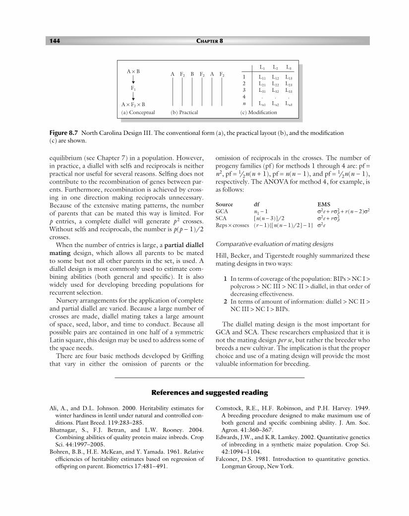
equilibrium (see Chapter 7) in a population. However,in practice, a diallel with selfs and reciprocals is neitherpractical nor useful for several reasons. Selfing does notcontribute to the recombination of genes between par-ents. Furthermore, recombination is achieved by cross-ing in one direction making reciprocals unnecessary.Because of the extensive mating patterns, the number of parents that can be mated this way is limited. For p entries, a complete diallel will generate p2 crosses.Without selfs and reciprocals, the number is p(p − 1)/2crosses.

When the number of entries is large, a partial diallelmating design, which allows all parents to be mated to some but not all other parents in the set, is used. Adiallel design is most commonly used to estimate com-bining abilities (both general and specific). It is alsowidely used for developing breeding populations forrecurrent selection.

Nursery arrangements for the application of completeand partial diallel are varied. Because a large number ofcrosses are made, diallel mating takes a large amount of space, seed, labor, and time to conduct. Because allpossible pairs are contained in one half of a symmetricLatin square, this design may be used to address some ofthe space needs.

There are four basic methods developed by Griffingthat vary in either the omission of parents or the

omission of reciprocals in the crosses. The number ofprogeny families (pf) for methods 1 through 4 are: pf =n2, pf = 1/2n(n + 1), pf = n(n − 1), and pf = 1/2n(n − 1),respectively. The ANOVA for method 4, for example, isas follows:

Source df EMSGCA n1 − 1 σ2e + rσ2

g + r(n − 2)σ2

SCA [n(n − 3)]/2 σ2e + rσ2g

Reps × crosses (r − 1){[n(n − 1)/2] − 1} σ2e

Comparative evaluation of mating designs

Hill, Becker, and Tigerstedt roughly summarized thesemating designs in two ways:

1 In terms of coverage of the population: BIPs > NC I >polycross > NC III > NC II > diallel, in that order ofdecreasing effectiveness.

2 In terms of amount of information: diallel > NC II >NC III > NC I > BIPs.

The diallel mating design is the most important forGCA and SCA. These researchers emphasized that it isnot the mating design per se, but rather the breeder whobreeds a new cultivar. The implication is that the properchoice and use of a mating design will provide the mostvaluable information for breeding.

144 CHAPTER 8

Figure 8.7 North Carolina Design III. The conventional form (a), the practical layout (b), and the modification (c) are shown.

References and suggested reading

Ali, A., and D.L. Johnson. 2000. Heritability estimates forwinter hardiness in lentil under natural and controlled con-ditions. Plant Breed. 119:283–285.

Bhatnagar, S., F.J. Betran, and L.W. Rooney. 2004.Combining abilities of quality protein maize inbreds. CropSci. 44:1997–2005.

Bohren, B.B., H.E. McKean, and Y. Yamada. 1961. Relativeefficiencies of heritability estimates based on regression ofoffspring on parent. Biometrics 17:481–491.

Comstock, R.E., H.F. Robinson, and P.H. Harvey. 1949. A breeding procedure designed to make maximum use ofboth general and specific combining ability. J. Am. Soc.Agron. 41:360–367.

Edwards, J.W., and K.R. Lamkey. 2002. Quantitative geneticsof inbreeding in a synthetic maize population. Crop Sci.42:1094–1104.

Falconer, D.S. 1981. Introduction to quantitative genetics.Longman Group, New York.

A × B

F1

A × F2 × B

L1

L11

L21

L31

.Ln1

L2

L12

L22

L32

.Ln2

L3

L13

L23

L33

.Ln3

1 2 3 4 n

A

(a) Conceptual (b) Practical (c) Modification

F2 B F2 A F2

POPC08 28/8/06 4:08 PM Page 144

Falconer, D.S., and T.F.C. Mackay. 1996. Introduction toquantitative genetics, 4th edn. Longman, Harlow, UK.

Gardner, C.O. 1977. Quantitative genetic studies and popula-tion improvement in maize and sorghum. In: Proceedingsof the International Conference on Quantitative Genetics(Pollak, E., O. Kempthorne, and T.B. Bailey, eds). IowaState University, Ames, IA.

Glover, M.A., D.B. Willmot, L.L. Darrah, B.E. Hibbard, andX. Zhu. 2005. Diallel analysis of agronomic traits usingChinese and US maize germplasm. Crop Sci. 45:1096–1102.

Griffing, B. 1956a. A generalized treatment of the use of dial-lel crosses in quantitative inheritance. Heredity 10:31–50.

Griffing, B. 1956b. Concept of general and specific combiningability in relation to a diallel crossing system. Aust. J. Biol.Sci. 9:463–493.

Henderson, C.R. 1963. Selection index and expected geneticadvance. In: Statistical genetics and plant breeding(Hanson, W.D., and H.F. Robinson, eds). NationalAcademy of Sciences and National Research CouncilPublication No. 982. National Academy of Sciences andNational Research Council, Washington, DC.

Hill, J., H.C. Becker, and P.M.A. Tigerstedt. 1998.Quantitative and ecological aspects of plant breeding.Chapman & Hall, London.

Holland, J.B. 2001. Epistasis and plant breeding. Plant Breed.Rev. 21:27–92.

Lin, C.Y. 1978. Index selection for genetic improvement ofquantitative characters. Theor. Appl. Genet. 52:49–56.

INTRODUCTION TO QUANTITATIVE GENETICS 145

Outcomes assessment

Part A

Please answer the following questions true or false:

1 Quantitative traits are more influenced by the environment than qualitative traits.2 Quantitative traits are controlled by polygenes.3 Heritability is a population phenomenon.4 The specific combining ability of a trait depends on additive gene action.5 Polygenes have distinct and distinguishable effects.6 Quantitative variation deals with discrete phenotypic variation.7 Quantitative traits are also called metric traits.

Part B

Please answer the following questions:

1 What is quantitative genetics, and how does it differ from qualitative genetics?2 Give two specific assumptions of quantitative genetic analysis.3 Describe additive gene action.4 What is the heritability of a trait?5 What is the breeders’ equation?

Part C

Please write a brief essay on each of the following topics:

1 Discuss the role of the environment in quantitative trait expression.2 Discuss the concept of general worth of a plant.3 Discuss the concept of intuitive selection.4 Discuss the application of combining ability analysis in plant breeding.5 Discuss a method of estimating heritability of a trait.

POPC08 28/8/06 4:08 PM Page 145