price discrimination in a congestible bertrand duopoly · this is not the case under monopoly,...

Prices, capacities and service quality in a congestible Bertrand

duopoly*

Bruno De Borger and Kurt Van Dender♠

5/20/2005

Abstract

We study the duopolistic interaction between congestible facilities that supply perfect substitutes and that make sequential decisions on capacities and prices. The consumers’ time cost of accessing or using a facility is determined by the volume-capacity ratio. We analyze duopoly prices, capacities and service quality (defined as the inverse of time costs of using the facility) and compare the results to monopoly and first-best outcomes. Findings include the following. First, while price competition between duopolists is beneficial for consumers, introducing capacity competition is harmful. The duopolist offers lower service quality than the monopolist, who does provide the socially optimal quality level. Second, higher marginal costs of capacity may increase profits. Third, asymmetric Nash-equilibria may result even when firms are ex ante identical. More specifically, when capacity is cheap or demand is relatively inelastic, the only stable equilibria are asymmetric. In such an equilibrium, the large facility provides high quality at a high price, and the smaller facility offers lower quality at lower prices. In other words, there is endogenous product differentiation by ex ante identical firms. Keywords: congestion, price-capacity games, imperfect competition JEL code: D43, L13, L14, L86, L91, R40

* Earlier versions of this paper were presented at the AEA-meetings in Philadelphia (January 2005), the Center for the Study of Democracy at UCI (February 2005), and the Department of Economics at the University of Antwerp (May 2005). We thank Robin Lindsey for detailed comments. We are also grateful to Jan Bouckaert, André de Palma, Ken Small, Frank Verboven and Bert Willems for additional remarks. Chen Feng Ng provided valuable programming assistance. We acknowledge financial support from the Flemish Fund for Scientific Research and from the U.S. Department of Transportation and the California Department of Transportation, through the University of California Transportation Center. ♠ Bruno De Borger, Department of Economics, University of Antwerp, Belgium ([email protected]); Kurt Van Dender, Department of Economics, University of California, Irvine ([email protected]).

mailto:[email protected]

mailto:[email protected]

1. Introduction

Facilities like seaports, airports, internet access providers, and roads, are prone to

congestion. When the volume of simultaneous users increases and capacity is constant,

the time cost of using these facilities increases. More generally, the quality of the service

provided by a facility may decrease when it gets crowded. Facility management can

respond to quality deterioration by changing prices, but also by adapting the capacity of

the facility. This paper asks how capacity and price decisions are made for congestible

facilities in an oligopolistic market structure, and compares the oligopoly result to the

monopoly and the socially optimal outcome. More specifically, we study the duopolistic

interaction between congestion-prone facilities that supply perfect substitutes in the

framework of a sequential game. The facilities first decide simultaneously on capacities;

next, they simultaneously choose prices, given capacity decisions. Prices and capacities

jointly determine consumers’ time cost of accessing or using a particular facility. The

quality of service, defined as the inverse of time costs of using a facility, declines with

crowding.

The analysis of this paper is relevant to a number of situations. Competition

between airports in metropolitan areas (e.g. San Francisco Airport and Oakland Airport in

the San Francisco Bay Area) is one example. The airports are congestible, so that service

quality declines with the number of passengers and plane movements. If airport

management maximizes profits1, then price decisions and capacity choices will interact

with service quality (congestion). A second example relates to competition between

ports that serve the same hinterland (e.g. the ports of Long Beach and of Los Angeles in

Southern California, or the ports of Antwerp and Rotterdam in Western Europe). Here

too, port capacities and port charges can be chosen by the port authorities to maximize

profits. Competition between internet service providers is another example, although our

maintained no entry assumption is less straightforward in this case. The quality of

internet service can be measured as a weighted average of (mainly) download speed,

1 At present, many airports do not act as profit-maximizers, especially in the U.S., as they are constrained by regulation and by long run contracts with (dominant) carriers (FAA/OST, 1999). In a fully deregulated environment, market power deriving from airport congestion may be more likely to accrue to airports than to airlines. Moreover, the interaction between congestion, price and capacity decisions is present when airports maximize a weighted sum of revenues and output.

1

upload speed and mail processing speed; the capacity (computing power, disk space and

network capacity) that is required to keep quality constant is approximately a linear

function of the number of simultaneous users.2

The main insights of this paper are the following. First, we find that, at the Nash

equilibrium capacities and prices, service quality is below the socially optimal level.

This is not the case under monopoly, where pricing and capacity choices do result in the

socially optimal service quality. In other words, since in our model duopoly prices are

below monopoly prices we find that, while price competition between duopolists yields

benefits for consumers, capacity competition is harmful. Second, strategic interaction

between prices and capacities implies that higher marginal capacity costs may increase

duopoly profits. Third, the duopoly outcome may yield both symmetric and asymmetric

Nash equilibria. Specifically, when capacity costs are low or demand is fairly elastic, the

only stable equilibria are asymmetric. This results in endogenous product differentiation

by ex ante identical facilities. Duopolistic interaction by the congested facilities results in

a large facility that provides high quality at a high price, and a small facility with a

smaller market share and lower quality and prices.

Our analysis of price and capacity decisions in a homogenous goods duopoly as a

sequential game in capacities and prices builds upon earlier literature. Braid (1986) and

Van Dender (2005) study duopoly pricing decisions of congested facilities, but they do

not consider capacity adjustments. de Palma and Leruth (1989) do study a two-stage

game in capacities and prices; however, they focus on a discrete demand representation

(users either consume one or zero units of the good), which does not allow discussing the

role of specific model parameters in much detail.3 Baake and Mitusch (2004) develop a

model similar to ours, but they focus on the comparison between Cournot and Bertrand

models in the pricing stage of the game and do not study the possibility of multiple

equilibria. This paper provides a more detailed analysis of Bertrand pricing policies, it

pays more attention to the distortion of service quality in the duopoly case, it contains a

detailed numerical illustration of price, capacity and service quality levels under different

2 Personal communication with Francis Depuydt, Team Manager Integrated Service Platforms, Belgacom. 3 In their model, the Nash equilibrium in capacities will occur where capacities are restricted up to the point of zero consumer surplus.

2

market structures, and it analyzes the occurrence of multiple equilibria. Acemoglu and

Ozdazgar (2005) recently provide a detailed theoretical analysis of competition and

efficiency on network markets. Among other things, they show that more competition

among oligopolists can reduce efficiency on congested markets, and that pure strategy

equilibria may not exist, especially when congestion functions are highly nonlinear.

However, they exclusively focus on price competition, and do not consider capacity

competition.

Lastly, the sequential capacity-price game can be contrasted to the literature

evolving from the seminal paper by Kreps and Scheinkman (1983). They show that, with

an L-shaped marginal cost function and with an efficient capacity-sharing rule, the two-

stage capacity-price game yields the same result as a one-stage Cournot game in

quantities. Later papers, e.g. Maggi (1996), Dastidar (1995, 1997) and Boccard and

Wauthy (2000, 2004), find that this result does not hold when marginal production costs

increase before capacity is reached or when different sharing rules are used. In the

current paper an upward sloping user cost function in combination with the consumer

equilibrium constraint leads to ‘endogenous sharing’, as the distribution of output over

the facilities is determined within the model, rather than through an external sharing rule

(as is required in the homogenous goods case without congestion, in order to determine

the distribution of market demand over firms). Not surprisingly, in this context the two-

stage capacity-price game does not reduce to a one-stage Cournot game.

The paper is structured as follows. Section two contains the theoretical analysis.

Section three uses a numerical example to clarify the properties of the model and to

illustrate the role of various parameters. Section four concludes.

2. Analytical model

This section provides a detailed analysis of the capacity-price game where the

duopolists are assumed to be profit-maximizers. First, the structure of the model and the

reduced form demand system are laid out. Then the second stage (price competition)

and the first stage (capacity competition) of the duopoly game are analyzed. The duopoly

solution is compared to the monopoly outcome and to the social welfare optimum. Note

that we delegate technical details to appendix wherever appropriate. An alternative

3

objective function, in which the facilities maximize a weighted sum of profits and of

output, is considered in appendix as well.4

2.1. Structure of the model and reduced form demands

There are two facilities, A and B, providing identical services. Consumers’

aggregate marginal willingness to pay is described by a downward sloping linear inverse

demand function

( )A BG q qα β α β= − = − + q (1)

where is the number of simultaneous users of facility i . Consumers pay a

price

( , )iq i A B=

Ap to use facility A and Bp to use facility B. In addition, they incur a time cost,

which depends on their marginal time cost γ and on congestion, which is defined as the

ratio between the number of (simultaneous) users { }, ,iq i A B= and a facility’s capacity

{ }, ,iK i A B= . Congestion can be interpreted literally, as an increase in time costs, or it

can be taken to reflect quality of service; this declines as the facility gets crowded. Like

de Palma and Leruth (1989), we denote the inverse of capacity by iR , so that the time

cost at each facility is { }, ,i iq R i A Bγ = .5 The marginal cost of capacity, { }, ,ic i A B= , is

assumed to be constant.

Throughout, we assume an interior solution, in which case consumer equilibrium

requires that generalized prices (the sum of prices and time costs) at both locations are

equal to the marginal willingness to pay. The structural form of the demand system can

be written as:

[ ][ ]

A B A A

A B B B

G q q p q R

G q q p q R

γ

γ

+ = +

+ = +A

B

(2)

where G(.) is given by (1) above. System (2) implicitly defines the reduced form demand

functions that express demand at each facility as a function of prices and capacities at

4 Several authors (e.g., Starkie (2001) and Zhang and Zhang (2003)) indeed argue that output may be a relevant partial objective for many airports. 5 Using inverse capacity facilitates many of the derivations below.

4

both facilities. Using superscript r for the reduced form demand functions, they can be

written in general as:

( )( )

, , ,

, , ,

rA A A B A B

rB B A B A B

q q p p R R

q q p p R R

=

= (3)

To derive the impact of price and capacity changes on demand, we differentiate system

(2), write the result in matrix notation and apply Cramer’s rule. We obtain:

0rA

A

q Rp A

β γ∂ − − B= <∂

(4)

0rA

B

qp A

β∂= >

∂ (5)

( ) 0r

A BA

A

q RqR A

γ β γ− −∂= <

∂ (6)

0rA B

B

q qR A

βγ∂= >

∂ (7)

where

( )( ) 0A B A BA R R R Rγ γ β= + + >

Recalling that R indicates the inverse of capacity, the signs correspond to

intuition: ceteris paribus, a higher price at a particular facility reduces demand at that

facility and increases demand at the other; more capacity at a facility (i.e., conditional on

demand being constant, better service quality) increases demand at that facility and

reduces demand at the other.

2.2 Stage two: Nash equilibrium in prices

We take the point of view of facility A. Its objective is to maximize profits:

max A

Ap A A A

A

cp qR

π = −

where demand is given by (3). Using (4), the first-order condition

5

=0 r

rAA A

A

qp qp∂

+∂

(8)

yields the following pricing rule (one easily verifies that the second-order conditions are

satisfied as long as demand is downward sloping):

(.) (.)r r BA A A A

B

Rp q R qR

βγ γβ γ

= ++

(9)

A similar expression holds for facility B. Expression (9) is conceptually identical

to the ones obtained in Braid (1986), Verhoef at al. (1996), and Van Dender (2005).6 The

optimal price, conditional on capacities at both facilities, consists of two components.

The first one implies that each facility charges the marginal congestion cost at its facility,

i.e. consumers pay for the marginal reduction in quality of service that their presence at

the facility imposes on other (simultaneously present) users. The second component is a

positive markup; it increases when demand becomes less elastic and when the competing

facility is more congestible. Note that, in the Bertrand setting, congestion costs are the

only source of market power: with γ=0, prices are equal to marginal production costs

(normalized to zero). Otherwise said, in the absence of congestion costs, the textbook

Bertrand paradox is obtained: price equals marginal cost.

The pricing rule (9) gives an implicit representation of the price reaction function

of facility A, conditional on capacities. By analogy we derive the price reaction function

for B. Jointly the two reaction functions define the Nash equilibrium prices for given

capacities, denoted as ( ),NEA A Bp R R , ( ),NE

B A Bp R R , respectively. In appendix 1 we show

that the price equilibrium is unique and stable. Moreover, we unambiguously obtain:

0NEA

A

pR

∂>

∂ (10)

0NEA

B

pR

∂>

∂ (11)

6 None of these papers study the role of capacity and capacity competition. Verhoef et al. (1996) focus on the monopoly case but do allow for nonlinear demands and costs. Similarity of (9) to their result suggests that the expression also holds for more general specifications of demands and costs.

6

This says that a marginal capacity decrease at facility A as well as at facility B raises the

Nash-equilibrium prices at A. In other words, a more congestible system is characterized

by higher Nash-equilibrium prices.

2.3 Stage one: Nash equilibrium in capacities

The first order condition for profit maximization in stage 1 is:

2(.) 0NE r

rA AA A

A A

p dq cq pR dR R

∂ A

A

+ + =∂

(12)

where

0 0 0 0 0

r r r NE rA A A A A B

A A A A B

dq q q p q pdR R p R p R

< < > > >

∂ ∂ ∂ ∂ ∂= + +

NE

A∂ ∂ ∂ ∂ ∂ (13)

is the total effect of a capacity change in A on demand. It consists of the direct effect,

holding prices constant, and indirect effects through Nash equilibrium price adjustments

at the pricing stage of the game. The signs of the partial derivatives of the reduced form

demand system and of the Nash-equilibrium prices – indicated beneath the expressions –

were defined in (4), (5), (6), and in (10) and (11). It follows from (10) and (12) that the

sign of (13) is negative, i.e., the direct effect of capacity on reduced-form demand

dominates the indirect effects through price reactions of capacity changes. Hence,

marginally increasing RA – marginally decreasing capacity at A – reduces demand at A.

Expression (12) basically equates marginal cost and benefit of a capacity change.

Note that, combining (12) and (13) and using the first order condition for optimal pricing

behavior in A (see (9)), condition (12) for optimal capacity choice can be formulated

equivalently as follows:

2 0r r NEA A B A

A AA B A A

q q p cp pR p R R∂ ∂ ∂

+ + =∂ ∂ ∂

(14)

This shows that the decision to supply higher capacity depends on capacity costs per unit

(third term), on the extent to which capacity directly raises demand (first term), and on

the extent to which it reduces demand via price adjustments by the competitor (second

7

term): higher capacity in A reduces the Nash equilibrium price of the competitor B, which

in turn reduces demand in A.

Equation (14) implicitly defines the reaction function in capacity for facility A. It

explicitly depends on the competitor’s capacity, BR , and on the capacity cost Ac :

( , )RA A B AR R R c≡

where the reaction function is denoted by superscript ‘R’. Rewriting (14) in implicit

form:

2( , , ) 0r r NEA A B A

A B A A AA B A A

q q p cR R c p pR p R R

ψ ∂ ∂ ∂= + +

∂ ∂ ∂=

and applying the implicit function theorem, we immediately find that a higher capacity

costs shifts the reaction function upwards:

2

1 1 0A

A A

RcA

A R R A

Rc R

ψψ ψ

⎡ ⎤∂= − = − >⎢ ⎥∂ ⎣ ⎦

(15)

Note that ARψ is negative by the second order condition for profit maximization in

capacity.

The slope of the capacity reaction function is given by:

B

A

RRA

B R

RR

ψψ

∂= −

∂ (16)

In general, one expects the sign of this slope to be ambiguous because two opposite

forces are at play. More capacity in B provides A an incentive to defend its market share

by responding with a capacity increase as well. The size of this effect will depend on

capacity costs. However, higher capacity in B reduces Nash equilibrium prices at both

facilities. Firm A then has an incentive to reduce capacity in order to increase prices (and

at the same time deliberately creating extra congestion). However, despite the ambiguity

in general, we show in Appendix 2 that, given the linear specifications of demand and

cost functions, reaction functions in capacity are highly plausibly downward sloping. For

example, we show that the slope will necessarily be negative at a symmetric equilibrium

of the two-stage game.

We now turn to the impact of capacity costs on Nash equilibrium capacities and

prices. Note that at a Nash equilibrium of the first stage of the game we have:

8

( ,

( ,

NE R NE )

)A A B ANE R NEB B A B

R R R c

R R R c

≡

≡ (17)

Differentiating system (17) yields:

1

RA

NEA A

R RA BA

B A

RR c

R RcR R

∂∂ ∂

=∂ ∂∂ −∂ ∂

(18)

1

R RB A

NEA B

R RB

A BB

B A

R RR c R

R RcR R

∂ ∂∂ ∂ ∂

=∂ ∂∂ −∂ ∂

(19)

1

RB

NEB B

R RA BB

B A

RR c

R RcR R

∂∂ ∂

=∂ ∂∂ −∂ ∂

(20)

1

R RA B

NEB A

R RA

A BA

B A

R RR c R

R RcR R

∂ ∂∂ ∂ ∂

=∂ ∂∂ −∂ ∂

(21)

These expressions imply that, if reaction functions are downward sloping and the

denominator is positive so as to guarantee stability, an increase in the capacity cost in A

reduces the Nash equilibrium capacity in A and raises it in B. Moreover, under these

assumptions, (18)-(19) and simple algebra show that a simultaneous increase in capacity

costs in both A and B raises equilibrium values of NEAR and NE

BR .

The effect of capacity costs on the Nash equilibrium price at facility A is given

by:

NE NE NE NE NEA A A A

A A A B

dp p R p Rdc R c R c

∂ ∂ ∂ ∂= + B

A∂ ∂ ∂ ∂ (22)

The overall impact is the sum of two terms; the first one is positive, the second one is

negative, because capacity costs in A raise Nash equilibrium capacities in B. If the direct

effects dominate the indirect effects due to capacity adjustments at the other facility, a

capacity cost increase induces a facility to raise prices.

9

We conclude this section with an important remark. Unlike the price reaction

functions at stage two, the capacity reaction functions are nonlinear, so that multiple

equilibria may result. This issue will be illustrated in the numerical application.

Moreover, stability of equilibria is not guaranteed. Not surprisingly, capacity costs are

likely to be crucial in determining stability of equilibria, because they directly affect

slopes of the capacity reaction functions. To see this, use (16) to get:

2

2( )

B A

A B

A

R RR RR

A A

B A R

AR c cR c

ψ ψψ ψ

ψ

∂ ∂−

∂ ∂= −

∂ ∂∂

Simple algebra shows that 0BR

Acψ∂

=∂

and 3

2 0AR

A Ac Rψ∂

= − <∂

, so that we have

2

3 2

2( )( )

B

A

RRA

B A A R

RR c R

ψψ

∂= −

∂ ∂

If reaction functions are downward sloping then BRψ <0 so that higher capacity costs in A

raise the slope (i.e., make it less negative); it becomes smaller in absolute value. These

findings suggest that, starting from a symmetric stable equilibrium, sufficiently low

capacity costs may generate unstable symmetric equilibria. This useful insight will also

be illustrated in the numerical application.

2.4 Duopoly, monopoly and the social optimum

The comparison of different market structures provides further insight into the

effects of the oligopolistic interaction on which this paper focuses. In this subsection we

derive price and capacity rules for a monopolist and for a social welfare-maximizer.

Assume first that both facilities are operated by a single profit-maximizer. Profits are

given by:

, ,

( , , , )r ii i A B A B

i A B i A B i

cp q p p R RR= =

−∑ ∑

and maximized with respect to the two prices and capacity levels. In Appendix 3 we

show that the first-order conditions yield, after simple manipulation:

10

( ) { }, ,i A B i ip q q q R i A Bβ γ= + + ∈ (23)

{1/ 2

1 , ,ii i

q i A BR c

γ⎛ ⎞= ∈⎜ ⎟⎝ ⎠

} (24)

According to (23), the price at each facility is the sum of the marginal congestion cost at

that location (second term) and a term relating to the elasticity of demand. Comparing

to(9), it follows that the elasticity-related markup is higher than in the duopoly case.

According to (24), capacity – the inverse of Ri – is inversely related to the marginal cost

of capacity, it is increasing in the marginal value of time, and it is proportional to demand

at the facility. Because the monopolist fully controls all instruments, his choice of

capacity does not directly take account of effects on the equilibrium price. This contrasts

to the duopoly case, where capacity choices do affect the Nash equilibrium price through

strategic interactions.

Next, assume the facilities are operated by a welfare-maximizing government. It

maximizes the difference between total net surplus and total social costs:

[ ], ,0

( )iq

ii i

i A B i A B i

cG u du G p qR= =

⎛ ⎞ ⎛ ⎞− − +⎜ ⎟ ⎜⎜ ⎟ ⎝ ⎠⎝ ⎠

∑ ∑∫ ⎟

In Appendix 3, we derive the following price and capacity rules.

{ }, ,i i ip q R i A Bγ= ∈ (25)

{1/ 2

1 , ,ii i

q i A BR c

γ⎛ ⎞= ∈⎜ ⎟⎝ ⎠

} (26)

Social welfare maximization internalizes the externality: the price equals the marginal

external congestion cost. The capacity rule is identical to that of the monopoly case (but

as it holds at a different price and a different level of demand, the optimal capacity level

will be different). Note that, since there are constant returns to scale in the provision of

capacity, optimal pricing and optimal provision of capacity lead to exact cost recovery

(see, e.g., Small (1992)). This follows because (25) implies total revenues equal to

2i i i i

i ip q q Rγ=∑ ∑ , and (26) allows us to write total expenditures as 2i

i ii ii

c q RR

γ=∑ ∑ .

Self-financing facilities imply that the social welfare maximum can be implemented

11

without distortionary taxes, viz. by a combination of congestion tolls and competitive

pricing at each facility. The competitive price equals the marginal private production cost

at each facility (here normalized to zero).

Comparing prices, capacity levels and quality of service under the three market

structures in more detail leads to a number of observations. First, while capacity levels

differ between the monopoly outcome and the social welfare maximum, the quality levels

(as measured by time costs of using a facility, i iR qγ ) are identical. To see this, note that

the optimal capacity rules (24) and (26) imply that, both under monopoly and at the social

welfare optimum, the time cost equals

(27) 1/ 2( )i i iR q cγ γ=

Hence, a monopolist has no incentive to distort quality, as all benefits of providing it

accrue to the facility itself. This observation is consistent with Spence (1975) 7, who

clarifies that the result is contingent on the additive structure of the generalized price.

Second, whereas a monopolist does not distort quality compared to the social

optimum, a duopolist unambiguously provides lower quality. To show this formally,

combine the first-order conditions for the optimal price and the optimal capacity level

(expressions (8) and (14), respectively) for facility A, and use (4), (5) and (6). This leads

to:

2

NEB A

A AB A

p cq qAR R R

βγβ γ

⎡ ⎤⎛ ⎞ ∂− =⎢ ⎥⎜ ⎟+ ∂⎝ ⎠⎣ ⎦

Multiplying both sides by ( 2ARγ ) and slightly manipulating the result yields:

[ ]( )1/ 2A A AR q c Zγ γ= + (28)

where [ ]2

0NE

A A B

B A

q R pZR R

γββ γ

∂= >

+ ∂.

Comparing (28) and (27) shows that the time cost under duopoly will exceed the socially

optimal one. Hence the duopolist offers lower service quality.

7 Spence (1975) shows that quality at the monopolists’ output level is below (above) the socially optimal level when the partial derivative of willingness to pay with respect to output and to quality is negative (positive). In our linear and additive specification of demand this derivative is zero, so that the monopolist supplies optimal quality.

12

The intuition for this finding lies in the strategic price responses to capacity

changes under duopoly. A capacity increase reduces the generalized cost and, therefore,

boosts demand at both facilities, implying that the benefits of a capacity increase at one

location partially accrue to the other. This externality is fully internalized in both the

social optimum and the monopoly case, but it is not under duopoly. In the latter case, for

example, a capacity increase at facility A affects not only capacity at the competing

facility B but also reduces the price there. The price reduction at the competing facility

negatively affects demand at A. Note that this strategic price response is clearly visible in

the term Z appearing in (28). If there was no price response to a capacity increase by the

competitor, Z=0 and the socially optimal service quality would result. The price response,

however, implies a ‘leakage of benefits’ of a capacity investment to the competitor to

which a facility reacts by providing less capacity than it otherwise would. The joint

implication of price and capacity choice is lower quality, as shown by (28). The

numerical analysis in the next section confirms this finding.

Third, together with (23) and (25), equal quality of service levels immediately

imply monopoly prices that necessarily exceed prices at the social optimum. Moreover,

with linear demands, duopoly prices will not only structurally but also numerically be

between those under monopoly and at the social optimum. Indeed, (8) implies that a

duopolist will operate where the price elasticity of reduced-form demand equals minus

one, whereas the monopolist operates at an elasticity exceeding one in absolute value.

3. Numerical analysis

This section explores the properties of the capacity-price game using

parameterized versions of the model analyzed in the previous section. All the scenarios

use ex ante symmetric parameterizations. Parameters were chosen to produce reasonable

elasticities of demand, but they do not reflect a particular real world empirical example.

In Section 3.1 we discuss a parameterization for which the model produces a

single, stable and symmetric Nash equilibrium (the ‘central scenario’). This scenario is

used to illustrate the sensitivity of the results to changes in economic parameters and to

compare the consequences of strategic interactions with monopoly and the welfare

13

optimum. Section 3.2 considers alternative values of marginal capacity costs, and

illustrates that ex ante symmetric parameterizations may lead to multiple Nash equilibria.

3.1 Central scenario: duopoly, monopoly and surplus maximization

Table 1 presents the parameters selected for the central scenario (rows 1 through

4) and the results (rows 5 through 21) for the unique and stable Nash-equilibrium of the

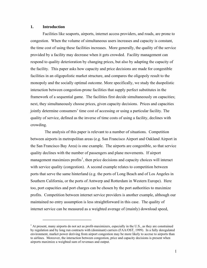
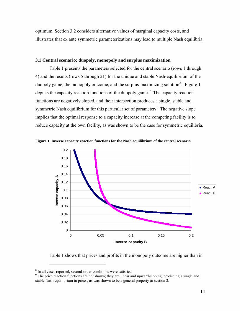
duopoly game, the monopoly outcome, and the surplus-maximizing solution8. Figure 1

depicts the capacity reaction functions of the duopoly game.9 The capacity reaction

functions are negatively sloped, and their intersection produces a single, stable and

symmetric Nash equilibrium for this particular set of parameters. The negative slope

implies that the optimal response to a capacity increase at the competing facility is to

reduce capacity at the own facility, as was shown to be the case for symmetric equilibria.

Figure 1 Inverse capacity reaction functions for the Nash equilibrium of the central scenario

0

0.02

0.04

0.06

0.08

0.1

0.12

0.14

0.16

0.18

0.2

0 0.05 0.1 0.15 0.2

Inverse capacity B

Inve

rse

capa

city

A

Reac. AReac. B

Table 1 shows that prices and profits in the monopoly outcome are higher than in

8 In all cases reported, second-order conditions were satisfied. 9 The price reaction functions are not shown; they are linear and upward-sloping, producing a single and stable Nash equilibrium in prices, as was shown to be a general property in section 2.

14

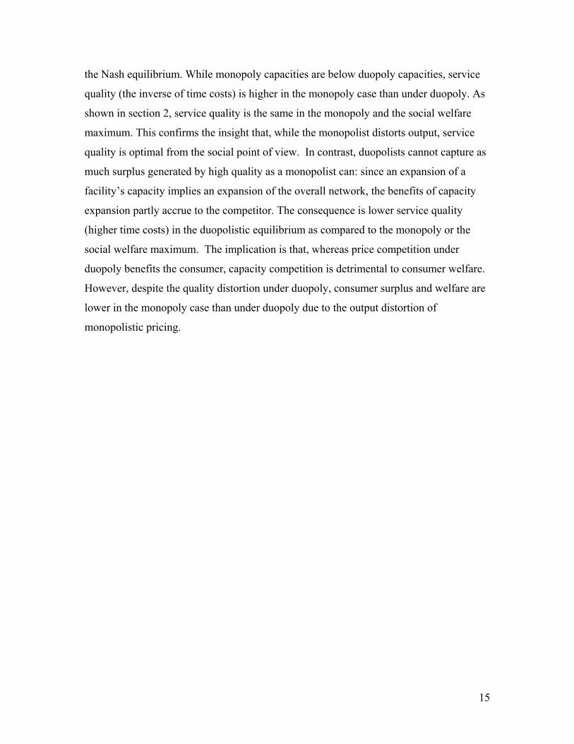
the Nash equilibrium. While monopoly capacities are below duopoly capacities, service

quality (the inverse of time costs) is higher in the monopoly case than under duopoly. As

shown in section 2, service quality is the same in the monopoly and the social welfare

maximum. This confirms the insight that, while the monopolist distorts output, service

quality is optimal from the social point of view. In contrast, duopolists cannot capture as

much surplus generated by high quality as a monopolist can: since an expansion of a

facility’s capacity implies an expansion of the overall network, the benefits of capacity

expansion partly accrue to the competitor. The consequence is lower service quality

(higher time costs) in the duopolistic equilibrium as compared to the monopoly or the

social welfare maximum. The implication is that, whereas price competition under

duopoly benefits the consumer, capacity competition is detrimental to consumer welfare.

However, despite the quality distortion under duopoly, consumer surplus and welfare are

lower in the monopoly case than under duopoly due to the output distortion of

monopolistic pricing.

15

Table 1 Parameters and solutions of the central scenario under alternative assumptions on market structure

Parameter or variable Symbol Duopoly: Nash

equilibrium

Monopoly Surplus maximization

1. Intercept inverse demand function α 13.8 2. Slope inverse demand function β 0.2 3. Marginal value of time γ 1 4. Marginal cost of capacity c 1 5. Quantity demanded q 47.671 29.500 59.000 6. Quantity demanded at A q

A23.836 14.750 29.500

7. Quantity demanded at B qBB

23.836 14.750 29.500

8. Generalized price g 4.266 7.900 2.000 9. Price at A p

A2.717 6.900 1.000

10. Price at B pBB

2.717 6.900 1.000

11. Time cost to A aA

1.548 1.000 1.000

12. Time cost to B aBB

1.548 1.000 1.000

13. Inverse capacity at A RA

0.065 0.068 0.0339

14. Inverse capacity at B RBB

0.065 0.068 0.0339

15. Capacity at A KA

15.393 14.749 29.500

16. Capacity at B KBB

15.393 14.749 29.500

17. Profits at A πA

49.375 87.025 0

18. Profits at B πBB

49.375 87.025 0

19. Generalized price elast. εQG

-0.45 -1.34 -0.17

20. Money price elast. at A εQPA

-0.29 -1.17 -0.08

21. Money price elast. at B εQPB

-0.29 -1.17 -0.08

Table 2 shows the implications of reducing the marginal value of time or raising

the marginal cost of capacity. Compared to Table 1, in Table 2 we have reduced, first,

the value of time and, second, the capacity cost from 1 to 0.5. The linear structure of the

model implies that the effects of an equal percentage reduction in the marginal value of

time or in the marginal cost of capacity on the relevant properties of the equilibrium are

identical.10 Intuitively, reducing the value of time directly reduces the time cost of

congestion; reducing capacity costs indirectly reduces the cost of congestion by raising

10 A reduced value of time implies that physical congestion levels are less costly, while a reduced marginal cost of capacity implies that alleviating congestion is cheaper. The latter leads to higher capacity levels in the social surplus maximum.

16

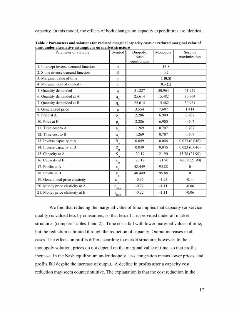
capacity. In this model, the effects of both changes on capacity expenditures are identical. Table 2 Parameters and solutions for reduced marginal capacity costs or reduced marginal value of time, under alternative assumptions on market structure


equilibrium


1. Intercept inverse demand function α 13.8 2. Slope inverse demand function β 0.2 3. Marginal value of time γ 1 (0.5) 4. Marginal cost of capacity c 0.5 (1) 5. Quantity demanded q 51.227 30.964 61.929 6. Quantity demanded at A q

A25.614 15.482 30.964


25.614 15.482 30.964


A2.286 6.900 0.707

10. Price at B pBB

2.286 6.900 0.707


1.269 0.707 0.707


1.269 0.707 0.707


0.049 0.046 0.023 (0.046)


0.049 0.046 0.023 (0.046)


20.19 21.90 43.78 (21.90)


20.19 21.90 43.78 (21.90)


48.449 95.88 0


48.449 95.88 0

19. Generalized price elasticity εQG

-0.35 -1.23 -0.11

20. Money price elasticity at A εQPA

-0.22 -1.11 -0.06

21. Money price elasticity at B εQPB

-0.22 -1.11 -0.06

We find that reducing the marginal value of time implies that capacity (or service

quality) is valued less by consumers, so that less of it is provided under all market

structures (compare Tables 1 and 2). Time costs fall with lower marginal values of time,

but the reduction is limited through the reduction of capacity. Output increases in all

cases. The effects on profits differ according to market structure, however. In the

monopoly solution, prices do not depend on the marginal value of time, so that profits

increase. In the Nash equilibrium under duopoly, less congestion means lower prices, and

profits fall despite the increase of output. A decline in profits after a capacity cost

reduction may seem counterintuitive. The explanation is that the cost reduction in the

17

provision of capacity reduces costs and raises demand at given prices, but it also

intensifies competition and reduces prices, indirectly reducing revenues. If the latter

effect dominates, lower capacity costs reduce profits.11 With regard to reductions in

values of time, comparison of Tables 1 and 2 shows that profits fall as values of time fall.

Since the opportunity cost of time increases with economic growth, this can be

interpreted as saying that congestion as a source of market power becomes more

important as the economy grows.

In Table 3 we look at the implications of changes in the slope of the demand

function. We find that prices, time costs and, therefore, generalized prices are not

affected at all (compare Tables 1 and 3). This is related to the linear structure of the

model. With linear congestion, demand and capacity cost functions, setting β at half its

initial value induces facilities to provide twice the initial capacity at twice the initial

output, and time costs remain constant. Note that the result is contingent on the two-stage

structure of the game, allowing firms to adjust capacities: in a one-stage pricing game

with constant capacities the Bertrand price does directly depends on the slope of the

demand function (Van Dender, 2005). Although the perfect proportionality of

adjustments in capacity and demand is specific to the linear model structure (more

specifically, to the additive structure of the generalized price and to the constant returns

in the provision of capacity), we expect prices not to be very sensitive to how demand

responds to cost increases in more general models as well. The intuition for the result is

simply that providing capacity contributes more to profit when demand is more sensitive

to reductions in time costs, so that more capacity is provided.

The above implies that the price elasticity of the (structural) demand function is

independent of the slope of the inverse demand function under each assumption on

market structure, see Tables 1 and 3. Given the linear demand function, it is clear that its

absolute value is largest (and above one) in the monopoly outcome, smaller in the

duopoly, and smallest in the welfare maximum.

11 One easily shows that the effect of a capacity cost increase may raise or reduce profit of a facility depending on the size of the different effects mentioned above. So the finding in Table 2 is not a general result. For example, an increase in capacity costs starting from relatively high initial capacity cost levels does reduce profits.

18

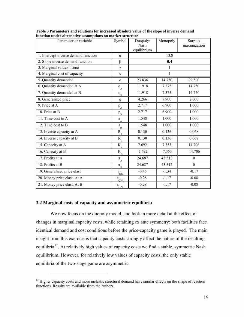
Table 3 Parameters and solutions for increased absolute value of the slope of inverse demand function under alternative assumptions on market structure


equilibrium


1. Intercept inverse demand function α 13.8 2. Slope inverse demand function β 0.4 3. Marginal value of time γ 1 4. Marginal cost of capacity c 1 5. Quantity demanded q 23.836 14.750 29.500 6. Quantity demanded at A q

A11.918 7.375 14.750


11.918 7.375 14.750


A2.717 6.900 1.000

10. Price at B pBB

2.717 6.900 1.000


1.548 1.000 1.000


1.548 1.000 1.000


0.130 0.136 0.068


0.130 0.136 0.068


7.692 7.353 14.706


7.692 7.353 14.706


24.687 43.512 0


24.687 43.512 0


-0.45 -1.34 -0.17

20. Money price elast. At A εQPA

-0.28 -1.17 -0.08

21. Money price elast. At B εQPB

-0.28 -1.17 -0.08

3.2 Marginal costs of capacity and asymmetric equilibria We now focus on the duopoly model, and look in more detail at the effect of

changes in marginal capacity costs, while retaining ex ante symmetry: both facilities face

identical demand and cost conditions before the price-capacity game is played. The main

insight from this exercise is that capacity costs strongly affect the nature of the resulting

equilibria12. At relatively high values of capacity costs we find a stable, symmetric Nash

equilibrium. However, for relatively low values of capacity costs, the only stable

equilibria of the two-stage game are asymmetric.

12 Higher capacity costs and more inelastic structural demand have similar effects on the shape of reaction functions. Results are available from the authors.

19

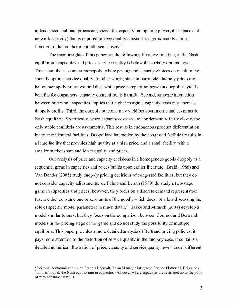
When marginal costs of capacity decline, the capacity reaction functions become

more convex and steeper in the neighborhood of the symmetric Nash-equilibrium, as is

illustrated in Figure 2. The symmetric intersections of these reaction functions are on a

ray through the origin. For relatively high capacity costs the reaction functions intersect

once and produce a single symmetric Nash equilibrium. Increased convexity at low

marginal capacity costs implies that, below a threshold value for marginal capacity costs,

the symmetric equilibrium becomes unstable. The model then yields multiple

intersections, and stable asymmetric equilibria result.

Figure 2 Inverse capacity reaction functions for various marginal capacity cost levels

0

0.02

0.04

0.06

0.08

0.1

0.12

0.14

0 0.01 0.02 0.03 0.04 0.05 0.06 0.07 0.08 0.09 0.1

Inverse capacity B

Inve

rse

capa

city

A c = 1c = 0.75c = 0.5

c = 0.25

c =0.1

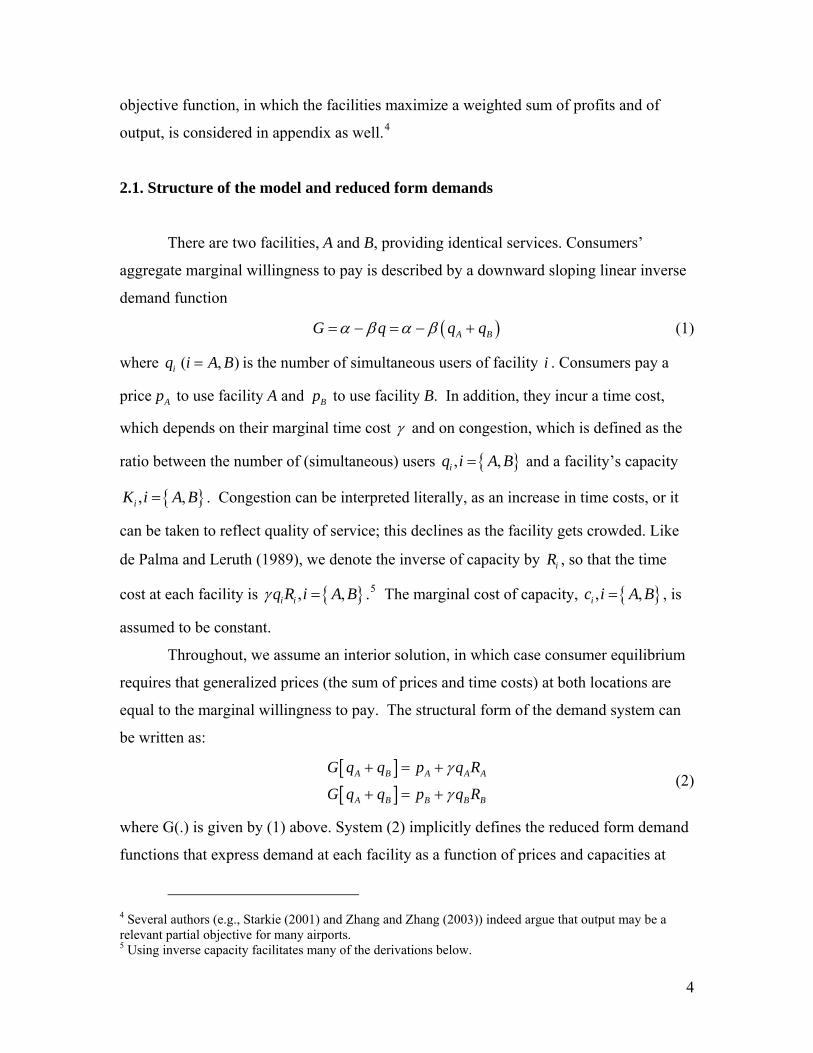
To illustrate the existence of multiple asymmetric equilibria at low capacity costs,

Figure 3 shows the reaction functions for both facilities for the case where marginal

capacity costs have been reduced to 0.25, keeping all other parameters at the level of the

central scenario. It shows that there are three Nash equilibria, of which the asymmetric

ones are stable. Table 4 shows the (unstable) symmetric and the stable asymmetric

equilibria. Total output in the latter equilibria is slightly lower than in the symmetric

20

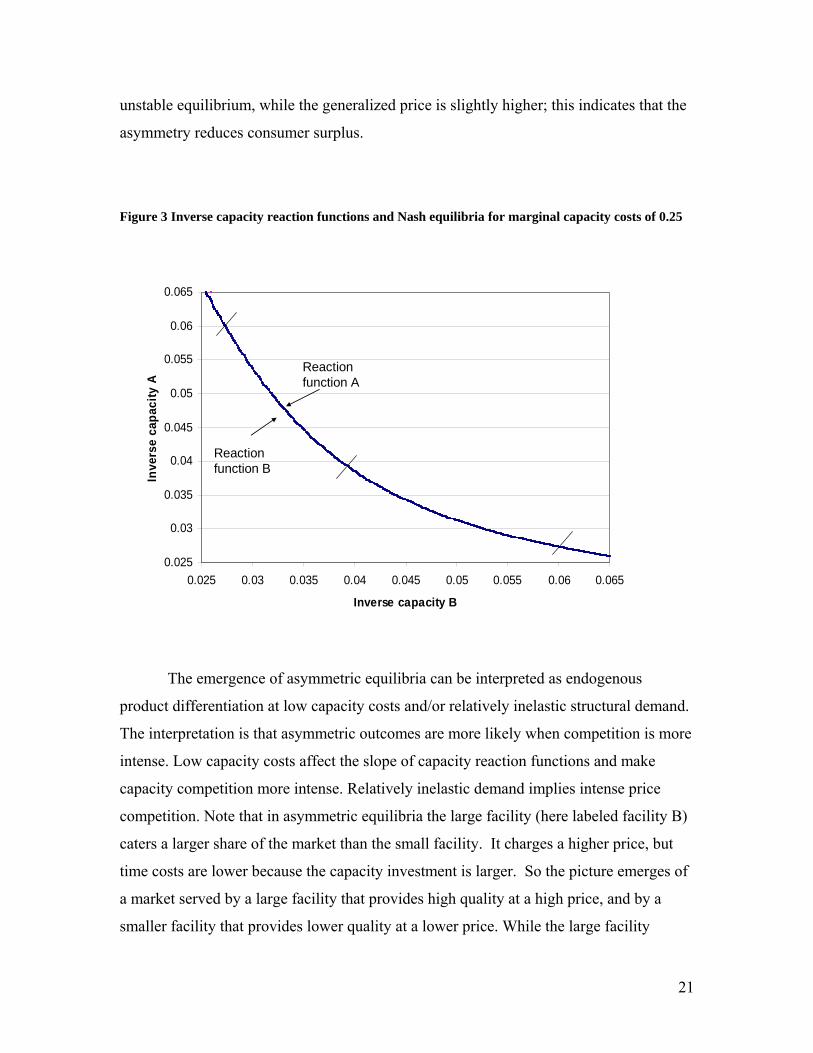
unstable equilibrium, while the generalized price is slightly higher; this indicates that the

asymmetry reduces consumer surplus.

Figure 3 Inverse capacity reaction functions and Nash equilibria for marginal capacity costs of 0.25

0.025

0.03

0.035

0.04

0.045

0.05

0.055

0.06

0.065

0.025 0.03 0.035 0.04 0.045 0.05 0.055 0.06 0.065

Inverse capacity B

Inve

rse

capa

city

A

RARB

Reaction function A

Reaction function B

The emergence of asymmetric equilibria can be interpreted as endogenous

product differentiation at low capacity costs and/or relatively inelastic structural demand.

The interpretation is that asymmetric outcomes are more likely when competition is more

intense. Low capacity costs affect the slope of capacity reaction functions and make

capacity competition more intense. Relatively inelastic demand implies intense price

competition. Note that in asymmetric equilibria the large facility (here labeled facility B)

caters a larger share of the market than the small facility. It charges a higher price, but

time costs are lower because the capacity investment is larger. So the picture emerges of

a market served by a large facility that provides high quality at a high price, and by a

smaller facility that provides lower quality at a lower price. While the large facility

21

grosses a larger profit, profit per unit of capacity investment is larger at the small facility

(2.17 instead of 1.71 at the large facility).

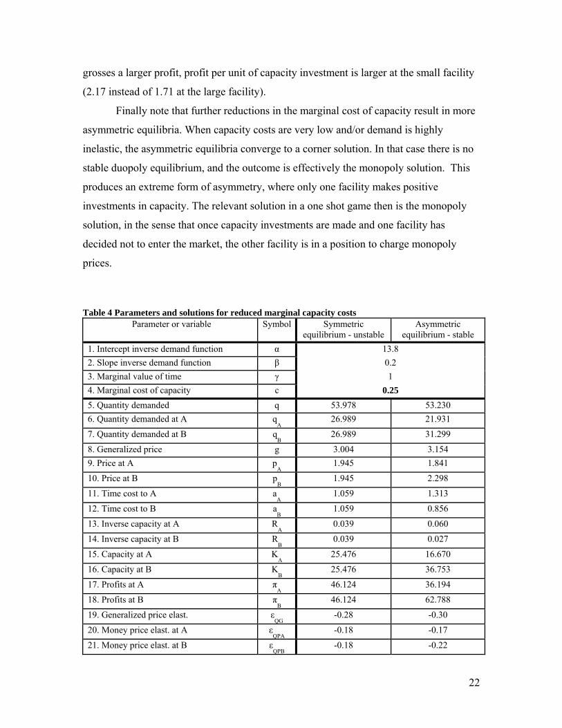
Finally note that further reductions in the marginal cost of capacity result in more

asymmetric equilibria. When capacity costs are very low and/or demand is highly

inelastic, the asymmetric equilibria converge to a corner solution. In that case there is no

stable duopoly equilibrium, and the outcome is effectively the monopoly solution. This

produces an extreme form of asymmetry, where only one facility makes positive

investments in capacity. The relevant solution in a one shot game then is the monopoly

solution, in the sense that once capacity investments are made and one facility has

decided not to enter the market, the other facility is in a position to charge monopoly

prices. Table 4 Parameters and solutions for reduced marginal capacity costs

Parameter or variable Symbol Symmetric equilibrium - unstable

Asymmetric equilibrium - stable

1. Intercept inverse demand function α 13.8 2. Slope inverse demand function β 0.2 3. Marginal value of time γ 1 4. Marginal cost of capacity c 0.25 5. Quantity demanded q 53.978 53.230 6. Quantity demanded at A q

A26.989 21.931


26.989 31.299

8. Generalized price g 3.004 3.154 9. Price at A p

A1.945 1.841

10. Price at B pBB

1.945 2.298


1.059 1.313


1.059 0.856


0.039 0.060


0.039 0.027


25.476 16.670


25.476 36.753


46.124 36.194


46.124 62.788


-0.28 -0.30

20. Money price elast. at A εQPA

-0.18 -0.17

21. Money price elast. at B εQPB

-0.18 -0.22

22

4. Concluding remarks

This paper has studied the duopolistic interaction between congestible facilities

that supply perfect substitutes and that make sequential decisions on capacities and

prices. Congestion increases consumers’ time costs of using a facility – alternatively, it

reduces the quality of service - and is determined by the ratio of the number of users and

capacity. Comparison of the duopoly outcome to the monopoly and the surplus

maximizing results leads to a number of insights. First, capacity provision and service

quality are less than socially optimal in the duopoly solution. This contrasts with the

monopoly outcome, where pricing and capacity provision are such that the monopolist

provides the socially optimal level of service quality. Since duopoly prices are lower than

monopoly prices we find that, whereas price competition between duopolists yields

benefits for consumer, capacity competition is harmful. Second, higher marginal capacity

costs may raise profits. Third, asymmetric Nash-equilibria may result even when firms

are ex ante identical. More specifically, when capacity is cheap or demand is relatively

inelastic, the only stable equilibria are asymmetric. In such an asymmetric equilibrium,

there is one large facility that provides high quality at a high price, and a small facility

with a smaller market share and lower quality and prices. This implies endogenous

product differentiation by ex ante identical facilities.

References

Acemoglu, Daron, and Asuman Ozdaglar. 2005. “Competition and efficiency in

congested markets,” NBER Working Paper 11201

Baake, Pio, and Kay Mitusch. 2004. “Competition with congestible networks,” DIW

Discussion Paper 402, Berlin

Boccard, Nicolas, and Xavier Wauthy. 2000. “Bertrand competition and Cournot

outcomes: further results,” Economics Letters, 68, 279-285

Boccard, Nicolas, and Xavier Wauthy. 2004. “Bertrand competition and Cournot

outcomes: a correction,” Economics Letters, 84, 163-166

Braid, Ralph M. 1986. “Duopoly pricing of congested facilities,” Columbia Department

of Economics Working Paper No. 322

23

Dastidar, K.G. 1995. “Comparing Cournot and Bertrand equilibria in homogenous

markets,” Journal of Economic Theory, 75, 205-212

Dastidar, K.G. 1997. “On the existence of pure strategy Bertrand equilibria,” Economic

Theory, 5, 19-32

de Palma, André and Luc Leruth. 1989. “Congestion and game in capacity: a duopoly

analysis in the presence of network externalities,” Annales d’Economie et de

Statistique, 15/16, 389-407

FAA/OST. 1999. “Airport business practices and their impact on airline competition,”

FAA/OST Task Force Study

Kreps, David M., and Jose A. Scheinkman. 1983. “Quantity precommitment and

Bertrand competition yield Cournot outcomes,” Bell Journal of Economics, 14, 2,

326-337

Maggi, Giovanni. 1996. “Strategic trade policies with endogenous mode of competition,”

American Economic Review, 86, 1, 237-258

Small, K.A. 1992. “Urban Transportation Economics”, Harwood Publishers.

Spence, M. 1975. “Monopoly, quality, and regulation,” Bell Journal of Economics, 6,

417-429

Starkie, D. 2001. “Reforming UK airport regulation”, Journal of Transport Economics

and Policy, 35, 119-135

Van Dender, Kurt. 2005. “Duopoly prices under congested access,” Journal of Regional

Science, 45, 2, 343-362

Verhoef E.T., P. Nijkamp and P. Rietveld. 1996. “Second-best congestion pricing: the

case of an untolled alternative,” Journal of Urban Economics, 40, 3, 279-302

Zhang, A., and Y. Zhang. 2003. “Airport charges and capacity expansion: effects of

concessions and privatization”, Journal of Urban Economics, 53, 54-75

24

Appendix 1. Properties of the price reaction functions and the Nash equilibrium

prices

The optimal pricing rules for A (see (9)) and its equivalent for B are implicit

representations of the price reaction functions (superscript R) ( ), ,R RA A B A Bp p p R R= and

( , ,R RB B A A B )p p p R R= , conditional on capacities. To find the slope of the price reaction

function for A, write the price rule in implicit form as follows:

( , , , ) ( , , , ) 0r BA B A B A A A B A B A

B

Rp p R R p q p p R R RR

γβω γβ γ

⎡ ⎤= − + =⎢ +⎣ ⎦

⎥ ,

where the dependence of demand on capacities and prices, see (3), has been made

explicit. Then use the implicit function theorem to find:

02( )

RA B

B B

A

p pp R

p

ωβ

ω β γ

∂∂ ∂= − = >

∂∂ +∂

(A1.1)

0RA A

A

A

p RR

p

ω

ω

∂∂ ∂= − =

∂∂∂

(A1.2)

2( ) 0

2( )

RA B

B B

A

p RR R

p

Bpω

γβ αω β γ

∂∂ −∂= − = >

∂∂ +∂

(A1.3)

Analogous results hold for B. As shown by (A1.1), the price reaction functions,

conditional on capacity, are linear in the price of the competing facility and upward

sloping. The slope is between zero and one, guaranteeing (given positive intercept, which

is easily shown to be the case) a unique interior Nash equilibrium in prices, for given

capacities. As is clear from(A1.3), the reaction of prices to capacities at the competitor’s

facility is not linear. As could be expected, the expression implies that a marginal

capacity decrease at B (i.e. a marginal increase in RB) leads to a higher price at A. B

Remarkably, equation (A1.2) shows that along the reaction function, a facility’s

price does not respond to a change in its capacity determined at the previous stage of the

game. Intuitively, there are two opposing effects from a marginal capacity increase. The

25

first one is that, holding demand in A constant, an increase in capacity in A reduces the

time cost in A, so reducing the optimal price. The second effect is that more capacity at A

increases demand in A, and this increases both the time cost and the markup, raising the

price. Given the specific model structure used (linear demands and congestion cost

functions), one easily shows that these two effects cancel out. Of course, in more general

models (e.g. with nonlinear congestion functions), the two effects will have opposite

signs but their absolute size need not be identical.

The Nash-equilibrium prices, for given capacities, are denoted ( ),NEA A Bp R R ,

( ),NEB A Bp R R , respectively. Formally, they are determined by the intersection of the

reaction functions:

( ) ( )( ) ( )

, ,

, ,

NE R NEA A B A B A B

NE R NEB A B B A A B

p R R p p R R

p R R p p R R

≡

≡

,

, (A1.4)

The sign of the effect of a marginal capacity increase at A and at B on these prices is

determined by differentiating system (A1.4). We find, using (A1.1)-(A1.3) and the

analogous effects for the reaction function in B:

01

R RA B

NEA B A

R RA BA

B A

p pp p R

p pRp p

∂ ∂∂ ∂ ∂

= >∂ ∂∂ −∂ ∂

(A1.5)

01

RA

NEA B

R RA BB

B A

pp R

p pRp p

∂∂ ∂

= >∂ ∂∂ −∂ ∂

(A1.6)

By (A1.1) and its equivalent for B, the denominator of these expressions is positive and

smaller than one. By (A1.1) and (A1.3), the numerator is positive.

Appendix 2 The slope of the capacity reaction functions

In this appendix we study the slope of the capacity reaction functions; in

particular, we show that at a symmetric Nash equilibrium of the two-stage game the

reaction functions of the capacity game are downward sloping.

The slope can be written in general as:

26

B

A

RRA

B R

RR

ψψ

∂= −

∂

where (.)ψ is the reaction function in implicit form defined in section 2.3, and ARψ is

negative by the second order condition for profit maximizing capacity choice. The

numerator can be written as:

2 2 2

B

r r NE NE r r r NE NENE A A B B A A A B

R AA

A B B A B A B B A B A

q q p p q q q p ppBR R p R R R p R R p R R

ψ⎡ ⎤ ⎡∂ ∂ ∂ ∂ ∂ ∂ ∂ ∂ ∂

= + + + +⎢ ⎥ ⎢∂ ∂ ∂ ∂ ∂ ∂ ∂ ∂ ∂ ∂ ∂ ∂⎣ ⎦ ⎣

⎤⎥⎦

(A2.1)

Using results derived earlier in the paper we obtain expressions for the individual terms

appearing in this equation.

First, differentiating (6) with respect to inverse capacity in B yields:

{2

2 2 31 ( )r

r r rAA B B B

A B

q q q q RR R A

β γ βγ∂= − −

∂ ∂} (A2.2)

where A >0 was defined in section 2.1. Note that the above expression is negative at an

ex post symmetric equilibrium ( rAq qr

B= ). At a sufficiently asymmetric equilibrium it

may be positive.

Second, differentiating the equivalent expression of (A1.6) for the price at B

yields:

2

2

2 0

1

R RA B

NEB B A A

R RA B A B

B A

p pp R p R

R R p pp p

∂ ∂∂ ∂ ∂ ∂

=∂ ∂ ⎛ ⎞∂ ∂

−⎜ ⎟∂ ∂⎝ ⎠

< (A2.3)

where the superscript ‘R’ refers to the reaction functions in prices at the second stage of

the game. Note that the expression is necessarily negative for our specification,

because 0RA

B

pR∂

>∂

(see (A1.3)) and, using the equivalent of (A1.3) for the price at B, we

easily show2 R

B

A A

pp R∂∂ ∂

<0.

27

Third, similar procedures as before easily show that:

( )( )

2

2 0r

AA

B B

Rqp R A

βγ β γ− +∂=

∂ ∂< (A2.4)

Again, this is negative. Moreover, from the first order condition of the capacity choice

problem (see (14)) we have that:

2 0r r NEA A B A

NEA B A A A

q q p cR p R p R∂ ∂ ∂

+ = −∂ ∂ ∂

< (A2.5)

Finally, earlier results reported in the paper imply:

0, 0, 0r NE NEA B A

B A B

q p pp R R∂ ∂ ∂

> > >∂ ∂ ∂

We have now determined the signs of all terms appearing in BRψ as given in

(A2.1). Using these results implies that the slope of the reaction function in capacities is

highly plausibly downward sloping. Unless (A2.2) is very largely positive (which

requires an extreme form of asymmetry) we have 0BRψ < , implying the slope of the

capacity reaction function is negative. At a symmetric equilibrium (so that (A2.2) is

necessarily negative), it follows that 0BRψ < . As a consequence, we have shown that, for

our specifications and at a symmetric equilibrium (we have used the first order conditions

of both the price and capacity game as well as the symmetry assumption to show the

result), the slope of the reaction function must be negative.

Appendix 3 The monopoly case and the social optimum

Assume first that both facilities are operated by a single profit-maximizer. Profits

are given by:

, ,

( , , , )r ii i A B A B

i A B i A B i

cp q p p R RR= =

−∑ ∑

and maximized with respect to the two prices and capacity levels. The first-order

conditions can be written as:

28

2 2

(.) 0; (.) 0

0; 0( ) ( )

r r r rr rA B A B

A A B A B BA A B Br r r rA B A A B B

A B A BA A A B B B

q q q qp q p p q pp p p p

q q c q q cp p p pR R R R R R

∂ ∂ ∂ ∂+ + = + + =

∂ ∂ ∂ ∂

∂ ∂ ∂ ∂+ + = + +

∂ ∂ ∂ ∂=

These equations can be manipulated, using the reduced-form derivatives derived before

(see (4)-(7) in the main body of the paper), to yield:

( ) { }, ,i A B i ip q q q R i A Bβ γ= + + ∈

{1/ 2

1 , ,ii i

q i A BR c

γ⎛ ⎞= ∈⎜ ⎟⎝ ⎠

}

Next, assume the facilities are operated by a welfare-maximizing government. It

maximizes the difference between total net surplus and total social costs:

[ ], ,0

( )iq

ii i

i A B i A B i

cG u du G p qR= =

⎛ ⎞ ⎛ ⎞− − +⎜ ⎟ ⎜⎜ ⎟ ⎝ ⎠⎝ ⎠

∑ ∑∫ ⎟

i

where, as before, demands are given by (3) and G is defined in (2). This last expression

implies

i iG p R qγ− =

Using this information, the first order conditions can be written as:

22

22

( 2 ) ( 2 ) 0; ( 2 ) ( 2 )

( 2 ) ( 2 ) 0( )

( 2 ) ( 2 ) 0( )

r r rA B A

A A B B A A B BA A B Br rA B A

A A B B AA A Ar rA B B

A A B B BB B B

q q q qG R q G R q G R q G R qp p p p

q q cG R q G R q qR R R

q q cG R q G R q qR R R

γ γ γ γ

γ γ γ

γ γ γ

∂ ∂ ∂ ∂− + − = − + −

∂ ∂ ∂ ∂

∂ ∂− + − − + =

∂ ∂

∂ ∂− + − − + =

∂ ∂

0rB =

B

Again using (2), we have 2 , ,i i i i iG R q p R q i Aγ γ− = − = . Substitution then

immediately implies the following price and capacity rules.

{ }, ,i i ip q R i A Bγ= ∈

{1/ 2

1 , ,ii i

q i A BR c

γ⎛ ⎞= ∈⎜ ⎟⎝ ⎠

}

29

Appendix 4 Alternative assumptions on firms’ objectives

Many congestible facilities (airport, ports, roads) are publicly owned or are

strongly regulated, so it is reasonable to consider objectives other than pure profit

maximization. For example, Starkie (2001) and Zhang and Zhang (2003) argue that

output is a relevant partial objective for many airports that generate revenues out of

concessions. Moreover, recent experiences in Europe also suggest that the social role of

airports encompasses more than profit, but that generating activities in itself is a valid

objective, for example, for reasons of employment opportunities. This section therefore

briefly explores the equilibria that result when facilities’ objectives consist of a weighted

sum of output and profit. When no weight is given to profits, the facilities are output

maximizers. When no weight is given to output, they are profit-maximizers, and the

analysis of the previous sections is obtained. Again, we look at look at alternative

ownership arrangements: duopoly refers to separate ownership of the facilities, monopoly

implies joint ownership13.

Duopoly: separate ownership

Suppose each facility is interested both in generating output (e.g. because of

lobbying by concessionary activities at an airport) and in profits. Assume that output and

profits receive an exogenous weight, normalize the output weight to one, and denote the

profit weight by μ>0.14 In stage 2 of the game, prices are set; the owner of facility A

maximizes:

AA A A

A

cq p qR

μ⎛ ⎞

+ −⎜⎝ ⎠

⎟

13 There is a potential semantic issue here, as duopoly and monopoly are usually understood to imply both a particular ownership structure and the profit maximization objective. Strictly speaking, when profit maximization is replaced by a different objective, one could argue that the duopoly and monopoly labels are no longer appropriate. We stick to this terminology, however, even under conditions of output maximizing behavior. 14 Using profits leads to the same results as using an exogenously defined allowable deficit.

30

subject to the consumer equilibrium constraints; i.e., demand in is given by the reduced-

form demands derived before. The first-order conditions lead to the following pricing

rule, conditional on capacities:

1BA A A A

B

Rp q R qR

βγ γβ γ μ

= ++

−

Compared to the case of profit-maximizing duopolists, see (9), the price rule is

amended by the extra term –1/μ. When this term is zero (i.e. as μ approaches infinity),

profits completely outweigh output in the objective, and (9) is obtained. When μ

becomes very small, output maximization becomes the main objective, and the last term

dominates, implying a subsidy (i.e., prices become negative). For smaller μ, strategic

interactions become relatively less important: output-maximization is obtained by

subsidies (and a complete disregard for congestion costs), whatever the other facility

does. In general, the strategic capacity setting decisions pertain to the profit-maximizing

part of the objective function, so that the structure of the first stage of the game (capacity

choices) is strongly similar to the profit-maximizing duopoly case.

Monopoly: joint ownership

Now consider joint ownership of both facilities; it maximizes:

, ,

ii i i

i A B i A B i

cq p qR

μ= =

⎛ ⎞+ ⎜

⎝ ⎠∑ ∑ − ⎟

subject to reduced-form demands, i.e., satisfying the consumer equilibrium constraints.

The corresponding price and capacity rules are:

1 ; , , ,i i ip q q R i j A B iβ γμ

= + − = ≠ j

121 ; ,i

i i

q i A BR c

γ⎛ ⎞= =⎜ ⎟⎝ ⎠

The capacity provision rule is the same as for a profit maximizing monopolist and

a social welfare maximizer. Not surprisingly, the price rule again reduces to that of a

31

profit maximizing monopolist when 1 0μ → . Interestingly, for 1qμ β= the welfare

maximizing rule is obtained. Intuitively, 1qμ β= indicates that output is not the only

objective (and becomes less important as output is high and β is large), because supply is

‘costly’.

We calculate the outcome of the model where a weighted sum of output and

profits is maximized under joint and separate ownership of the facilities, using the

parameters of the scenario with inelastic demand and high capacity costs. The key results

for various values of μ, the exogenous weight of profits, are summarized in Table A.4.1.

Table A.4.1 Key Results for mixed objective

Exogenous weight of profits in the objective function (μ) μ−−>+inf μ=1.5 μ=1 μ=0.5 μ−−>0 Separate ownership Output 51.8 52.1 52.2 52.7 56.9 Price 10.8 10.2 9.9 8.9 0.05 Time cost 5.67 5.69 5.71 5.75 6.14 Capacity 4.56 4.57 4.57 4.58 4.63 Single ownership Output 29.5 29.67 29.75 30.00 57.28 Price 60 59.67 59.50 59.00 4.4 Time cost 1 1 1 1 1 Capacity 14.75 14.83 14.87 15.00 28.64

In the leftmost column, the profit weight approaches infinity and the same results

are obtained as under pure duopoly and pure monopoly. When the relative weight of

output increases, output increases and prices decrease due to a lower weight on profit.

The difference between separate (duopoly) and single (monopoly) ownership lies in the

quality of service. With single ownership, the quality of service is independent (and

equal to the socially optimal level of quality) of the relative weights of profits and output.

In the duopoly case, putting more weight on output (reducing μ) leads to a deterioration

of the quality of service.

32

price discrimination in a congestible bertrand duopoly · this is not the case under monopoly,...

Documents