Profile-based Dynamic Voltage and Frequency Scaling for a Multiple ClockDomain Microprocessor

�

Grigorios Magklis�, Michael L. Scott

�, Greg Semeraro

�, David H. Albonesi

�, and Steven Dropsho

�

�Department of Computer Science�

Department of Electrical and Computer EngineeringUniversity of Rochester, Rochester, NY 14627

Abstract

A Multiple Clock Domain (MCD) processor addressesthe challenges of clock distribution and power dissipationby dividing a chip into several (coarse-grained) clock do-mains, allowing frequency and voltage to be reduced in do-mains that are not currently on the application’s criticalpath. Given a reconfiguration mechanism capable of choos-ing appropriate times and values for voltage/frequencyscaling, an MCD processor has the potential to achieve sig-nificant energy savings with low performance degradation.

Early work on MCD processors evaluated the poten-tial for energy savings by manually inserting reconfigura-tion instructions into applications, or by employing an ora-cle driven by off-line analysis of (identical) prior programruns. Subsequent work developed a hardware-based on-linemechanism that averages 75–85% of the energy-delay im-provement achieved via off-line analysis.

In this paper we consider the automatic insertion of re-configuration instructions into applications, using profile-driven binary rewriting. Profile-based reconfiguration in-troduces the need for “training runs” prior to productionuse of a given application, but avoids the hardware com-plexity of on-line reconfiguration. It also has the potentialto yield significantly greater energy savings. Experimen-tal results (training on small data sets and then running onlarger, alternative data sets) indicate that the profile-drivenapproach is more stable than hardware-based reconfigura-tion, and yields virtually all of the energy-delay improve-ment achieved via off-line analysis.

1. Introduction

The ongoing push for higher processor performance hasled to a dramatic increase in clock frequencies in recentyears. The Pentium 4 microprocessor is currently shippingat 3.06 GHz [27], and is designed to throttle back executionwhen power dissipation reaches 81.8W. At the same time,�This work was supported in part by NSF grants CCR–9701915,

CCR–9702466, CCR–9811929, CCR–9988361, CCR–0204344, and EIA–0080124; by DARPA/ITO under AFRL contract F29601-00-K-0182; by anIBM Faculty Partnership Award; and by equipment grants from IBM, Intel,and Compaq.

technology feature sizes continue to decrease, and the num-ber of transistors in the processor core continues to increase.As this trend toward larger and faster chips continues, de-signers are faced with several major challenges, includingglobal clock distribution and power dissipation.

It has been suggested that purely asynchronous systemshave the potential for higher performance and lower powercompared to fully synchronous systems. Unfortunately,CAD and validation tools for such designs are not yet readyfor industrial use. An alternative, which addresses all ofthe above issues, is a Globally Asynchronous Locally Syn-chronous (GALS) system [9]. In previous work we haveproposed a GALS system known as a Multiple Clock Do-main (MCD) processor [30]. Each processor region (do-main) is internally synchronous, but domains operate asyn-chronously of one another. Existing synchronous designtechniques can be applied to each domain, but global clockskew constraints are lifted. Moreover, domains can be givenindependent voltage and frequency control, enabling dy-namic voltage scaling at the level of domains.

Global dynamic voltage scaling already appears in manysystems, notably those based on the Intel XScale [25] andTransmeta Crusoe [17] processors, and can lead to signifi-cant reductions in energy consumption and power dissipa-tion for rate-based and partially idle workloads. The ad-vantage of an MCD architecture is its ability to save energyand power even during “flat out” computation, by slowingdomains that are comparatively unimportant to the appli-cation’s critical path, even when those domains cannot begated off completely.

The obvious disadvantage is the need for inter-domainsynchronization, which incurs a baseline performancepenalty—and resulting energy penalty—relative to a glob-ally synchronous design. We have quantified the perfor-mance penalty at approximately 1.3% [29]. Iyer and Mar-culescu [23] report a higher number, due to a less precise es-timate of synchronization costs. Both studies confirm thatan MCD design has a significant potential energy advan-tage, with only modest performance cost, if the frequenciesand voltages of the various domains are set to appropriatevalues at appropriate times. The challenge is to find an ef-fective mechanism to identify those values and times.

As with most non-trivial control problems, an optimalsolution requires future knowledge, and is therefore infeasi-ble. In a recent paper, we proposed an on-line attack-decayalgorithm that exploits the tendency of the future to resem-ble the recent past [29]. Averaged across a broad range ofbenchmarks, this algorithm achieved overall energy � delayimprovement of approximately 85% of that possible withperfect future knowledge.

Though a hardware implementation of the attack-decayalgorithm is relatively simple (fewer than 2500 gates), itnonetheless seems desirable to find a software alternative,both to keep the hardware simple and to allow differentcontrol algorithms to be used at different times, or for dif-ferent applications. It is also clearly desirable to close theenergy � delay gap between the on-line and off-line (futureknowledge) mechanisms. In this paper we address thesegoals through profile-driven reconfiguration.

For many applications, we can obtain a better predictionof the behavior of an upcoming execution phase by study-ing the behavior of similar phases in prior runs than we canfrom either static program structure or the behavior of re-cent phases in the current run. The basic idea in profile-driven reconfiguration is to identify phases in profiling runsfor which certain voltage and frequency settings would beprofitable, and then to modify the application binary to rec-ognize those same phases when they occur in productionruns, scaling voltages and frequencies as appropriate.

Following Huang [21], we assume that program phaseswill often be delimited by subroutine calls. We also con-sider the possibility that they will correspond to loop nestswithin long-running subroutines. We use traditional profil-ing techniques during training runs to identify subroutinesand loop nests that make contributions to program runtimeat a granularity for which MCD reconfiguration might beappropriate (long enough that a frequency/voltage changewould have a chance to “settle in” and have a potential im-pact; not so long as to suggest a second change). We thenemploy off-line analysis to choose MCD settings for thoseblocks of code, and modify subroutine prologues/epiloguesand loop headers/footers in the application code to effect thechosen settings during production runs.

Following Hunt [22], we accommodate programs inwhich subroutines behave differently when called in differ-ent contexts by optionally tracking subroutine call chains,possibly distinguishing among call sites within a given sub-routine as well. Experimentation with a range of options(Section 4) suggests that most programs do not benefit sig-nificantly from this additional sophistication.

The rest of the paper is organized as follows. In Sec-tion 2, we briefly review the MCD microarchitecture. InSection 3, we describe our profiling and instrumentation in-frastructure, and discuss alternative ways to identify corre-sponding phases of training and production runs. Perfor-

Front−end

Integer Floating−point

Memory

Main Memory

External

Integer Issue Queue

Int ALUs & Register File

FP Issue Queue

FP ALUs & Register File

Fetch Unit

L1 I−Cache

ROB, Rename, Dispatch L2 Cache

Load/Store Unit

L1 D−Cache

Figure 1. MCD processor block diagram.

mance and energy results appear in Section 4. Additionaldiscussion of related work appears in Section 5. Section 6summarizes our conclusions.

2. Multiple Clock Domain Microarchitecture

In our study, we use the MCD processor proposedin [30]. The architecture consists of four different on-chipclock domains (Figure 1) for which frequency and voltagecan be controlled independently. In choosing the bound-aries between them, an attempt was made to identify pointswhere (a) there already existed a queue structure that servedto decouple different pipeline functions, or (b) there wasrelatively little inter-function communication. Main mem-ory is external to the processor and for our purposes canbe viewed as another, fifth, domain that always runs at fullspeed.

The disadvantage of an MCD design is the need for syn-chronization when information crosses the boundary be-tween domains. The synchronization circuit is based onthe work of Sjogren and Myers [31]. It imposes a delayof one cycle in the consumer domain whenever the distancebetween the edges of the two clocks is within 30% of theperiod of the faster clock. Our simulator, derived from theone used in [30], includes a detailed model of the synchro-nization circuit, including randomization caused by jitter.

For the baseline processor, we assume a 1GHz clockand 1.2V supply voltage. We also assume a model of fre-quency and voltage scaling based on the behavior of the In-tel XScale processor [11], but with a tighter voltage range,reflecting expected compression in future processor genera-tions. A running program initiates a reconfiguration by writ-ing to a special control register. The write incurs no idle-time penalty: the processor continues to execute throughthe voltage/frequency change. There is, however, a delaybefore the change becomes fully effective. Traversing theentire voltage range requires 55 ��� . Given this transitiontime, changes will clearly be profitable only if performed at

a granularity measured in thousands of cycles.

3. Application Analysis

Our profile-based control algorithm can be divided intofour phases, which we discuss in the four subsections below.Phase one performs conventional performance profiling toidentify subroutines and loop nests that are of appropriatelength to justify reconfiguration. Phase two constructs aDAG that represents dependences among primitive opera-tions in the processor and then applies a “shaker” algorithmto distribute the slack in the graph in a way that minimizesenergy [30]. Phase three uses per-domain histograms ofprimitive operation frequencies to identify, for each chosensubroutine or loop nest, the minimum frequency for eachdomain that would, with high probability, allow executionto complete within a fixed slowdown bound. Phase fouredits the application binary to embed path-tracking or re-configuration instructions at the beginnings and ends of ap-propriate subroutines and loop nests.

3.1. Choosing Reconfiguration Points

Changing the domain voltage takes several microsec-onds and thus is profitable only over intervals measuredin thousands of instructions. Our goal is therefore to findthe boundaries between major application phases. Whileour previous off-line [30] and attack-decay [29] algorithmsmake reconfiguration decisions at fixed intervals, regardlessof program structure, it is clear that program phases corre-spond in practice to subroutine calls and loops [21], andthat the boundaries of these structures are the natural pointsat which to instrument program binaries for the purpose ofreconfiguration.

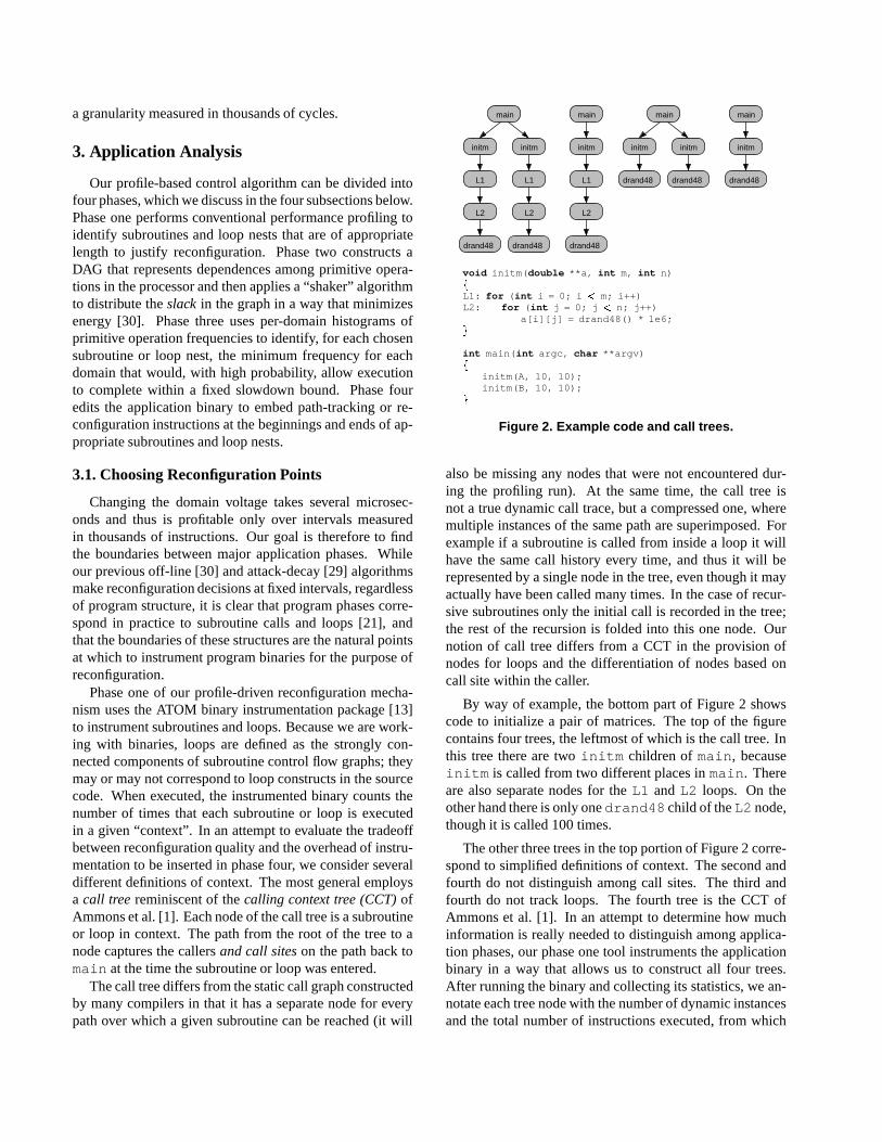
Phase one of our profile-driven reconfiguration mecha-nism uses the ATOM binary instrumentation package [13]to instrument subroutines and loops. Because we are work-ing with binaries, loops are defined as the strongly con-nected components of subroutine control flow graphs; theymay or may not correspond to loop constructs in the sourcecode. When executed, the instrumented binary counts thenumber of times that each subroutine or loop is executedin a given “context”. In an attempt to evaluate the tradeoffbetween reconfiguration quality and the overhead of instru-mentation to be inserted in phase four, we consider severaldifferent definitions of context. The most general employsa call tree reminiscent of the calling context tree (CCT) ofAmmons et al. [1]. Each node of the call tree is a subroutineor loop in context. The path from the root of the tree to anode captures the callers and call sites on the path back tomain at the time the subroutine or loop was entered.

The call tree differs from the static call graph constructedby many compilers in that it has a separate node for everypath over which a given subroutine can be reached (it will

drand48

L2

initm

L1

drand48

L2

initm

L1

main

drand48

L2

initm

L1

main main

initm initm

drand48 drand48

main

initm

drand48

void initm(double **a, int m, int n)�L1: for (int i = 0; i m; i++)L2: for (int j = 0; j n; j++)

a[i][j] = drand48() * 1e6;int main(int argc, char **argv)�

initm(A, 10, 10);initm(B, 10, 10);

Figure 2. Example code and call trees.

also be missing any nodes that were not encountered dur-ing the profiling run). At the same time, the call tree isnot a true dynamic call trace, but a compressed one, wheremultiple instances of the same path are superimposed. Forexample if a subroutine is called from inside a loop it willhave the same call history every time, and thus it will berepresented by a single node in the tree, even though it mayactually have been called many times. In the case of recur-sive subroutines only the initial call is recorded in the tree;the rest of the recursion is folded into this one node. Ournotion of call tree differs from a CCT in the provision ofnodes for loops and the differentiation of nodes based oncall site within the caller.

By way of example, the bottom part of Figure 2 showscode to initialize a pair of matrices. The top of the figurecontains four trees, the leftmost of which is the call tree. Inthis tree there are two initm children of main, becauseinitm is called from two different places in main. Thereare also separate nodes for the L1 and L2 loops. On theother hand there is only one drand48 child of the L2 node,though it is called 100 times.

The other three trees in the top portion of Figure 2 corre-spond to simplified definitions of context. The second andfourth do not distinguish among call sites. The third andfourth do not track loops. The fourth tree is the CCT ofAmmons et al. [1]. In an attempt to determine how muchinformation is really needed to distinguish among applica-tion phases, our phase one tool instruments the applicationbinary in a way that allows us to construct all four trees.After running the binary and collecting its statistics, we an-notate each tree node with the number of dynamic instancesand the total number of instructions executed, from which

5K

H

4K

I

3K

J

6K

K

20K

8K

G

20K

F

29K 4K

L

1K

M

2K

N

50K 19K

75K

B

D E

C

A

Figure 3. Call tree with associated instructioncounts. The shaded nodes have been identifiedas candidates for reconfiguration.

we can calculate the average number of instructions per in-stance (including instructions executed in the children of thenode). We then identify all nodes that run long enough fora frequency change to take effect and to have a potentialimpact on energy consumed. We use 10,000 instructions asthe definition of “long enough”. A longer window couldonly reduce the quality of reconfiguration, and would havea negligible impact on the instrumentation overhead.

Starting from the leaves and working up, we identify allnodes whose average instance (excluding instructions ex-ecuted in long-running children) exceeds 10,000. Figure 3shows a call tree in which the long-running nodes have beenshaded. Note that these nodes, taken together, are guar-anteed to cover almost all of the application history of theprofiled run (all that can be missing is a few short-runningnodes near the root).

We report results in Section 4 for six different defini-tions of context. Four correspond to the trees in the up-per portion of Figure 2. We call these L+F+C+P, L+F+P,F+C+P, and F+P, where F stands for “function” (subrou-tine), L stands for “loop”, C stands for “call site”, and Pstands for “path”. We also consider two simpler definitions,L+F and F, which use the L+F+P and F+P trees to identifylong-running nodes in phase one, but ignore calling historyduring production runs, allowing them to employ signifi-cantly simpler phase four instrumentation.

3.2. The Shaker Algorithm

To select frequencies and corresponding voltages forlong-running tree nodes, we use the “shaker” and “slow-down thresholding” algorithms from the off-line analysisof [30]. We run the application through a heavily-modifiedversion of the SimpleScalar/Wattch toolkit [4, 5], with allclock domains at full frequency. During this run we collecta trace of all primitive events (temporally contiguous workperformed within a single hardware unit on behalf of a sin-gle instruction), and of the functional and data dependencesamong these events. The output of the trace is a dependenceDAG for each long-running node in the call tree. Working

from this DAG, the shaker algorithm attempts to “stretch”(scale) individual events that are not on the application’scritical execution path, as if they could be run at their own,event-specific lower frequency.

Whenever an event in the dependence DAG has two ormore incoming arcs, it is likely that one arc constitutes thecritical path and that the others will have “slack”. Slackindicates that the previous operation completed earlier thannecessary. If all of the outgoing arcs of an event have slack,then we have an opportunity to save energy by performingthe event at a lower frequency. With each event in the DAGwe associate a power factor whose initial value is based onthe relative power consumption of the corresponding clockdomain in our processor model. When we stretch an eventwe scale its power factor accordingly.

The goal of the shaker is to distribute slack as uniformlyas possible. It begins at the end of the DAG and works back-ward toward the beginning. When it encounters a stretch-able event whose power factor exceeds the current thresh-old, originally set to be slightly below that of the few mostpower-intensive events in the graph (this is a high-powerevent), the shaker scales the event until either it consumesall the available slack or its power factor drops below thecurrent threshold. If any slack remains, the event is movedlater in time, so that as much slack as possible is movedto its incoming edges. When it reaches the beginning ofthe DAG, the shaker reverses direction, reduces its powerthreshold by a small amount, and makes a new pass forwardthrough the DAG, scaling high-power events and movingslack to outgoing edges. It repeats this process, alternatelypassing forward and backward over the DAG, reducing itspower threshold each time, until all available slack has beenconsumed, or until all events adjacent to slack edges havebeen scaled down to one quarter of their original frequency.When it completes its work, the shaker constructs a sum-mary histogram for each clock domain. Each histogram in-dicates, for each of the frequency steps, the total number ofcycles for events in the domain that have been scaled to runat or near that frequency. Histograms for multiple dynamicinstances of the same tree node are then combined, and pro-vided as input to the slowdown thresholding algorithm.

3.3. Slowdown Thresholding

Phase three of our profile-driven reconfiguration mech-anism recognizes that we cannot in practice scale the fre-quency of individual events: we must scale each domain asa whole. If we are willing to tolerate a small percentage per-formance degradation, � , we can choose a frequency thatcauses some events to run slower than ideally they might.Using the histograms generated by the shaker algorithm,we calculate, for each clock domain and long-running treenode, the minimum frequency that would permit the do-main to complete its work with no more than � % slow-

down. More specifically, we choose a frequency such thatthe sum, over all events in higher bins of the histogram, ofthe extra time required to execute those events at the chosenfrequency is less than or equal to � % of the total length ofall events in the node, run at their ideal frequencies. Thisdelay calculation is by necessity approximate. For mostapplications the overall slowdown estimate turns out to bereasonably accurate: the figures in Section 4 show perfor-mance degradation (with respect to the MCD baseline) thatis roughly in keeping with � .

3.4. Application Editing

To effect the reconfigurations chosen by the slowdownthresholding algorithm, we must insert code at the begin-ning and end of each long-running subroutine or loop. Forall but the L+F and F definitions of context, we must alsoinstrument all subroutines that appear on the call chain ofone or more long-running nodes. For the L+F+C+P andF+C+P definitions, we must instrument relevant call siteswithin such routines. In other words, reconfiguration pointsin the edited binary are a (usually proper) subset of the in-strumentation points.

To keep track of run-time call chains, we assign a staticnumeric label to each node in the tree, starting from � ( is aspecial label that means that we are following a path that didnot appear in the tree during training runs). We also assigna static label, from a different name space, to each subrou-tine that corresponds to one or more nodes in the tree. Ifthe nodes of a call tree are labeled from � to � , the cor-responding subroutines will be labeled from to ����� ,where ����� . In the most general case (L+F+C+P), weinstrument the prologue of each of the � subroutines thatparticipate in the tree to access an ������������� lookuptable, using the label of the previous node at run time (heldin a global variable) and the label of the current subroutine(held in a static constant in the code) to find the new nodelabel. Subroutine epilogues restore the previous value.

Headers and footers of long-running loops are also in-strumented, as are call sites that may lead to long-runningnodes (assuming we’re tracking call sites), but these do notneed to use the lookup table. It is easy to guarantee thatthe label of every loop and call site differs by a staticallyknown constant from the label of the subroutine in which itappears. To obtain the new node label, a loop header or callsite can simply add an offset to the current label.

We also generate an ����� -entry table containing the fre-quencies chosen by the slowdown thresholding algorithm ofphase three. When entering a subroutine (or loop) that cor-responds to one or more long-running nodes, we use thenewly calculated node label to index into this table. Wethen write the value found into an MCD hardware recon-figuration register. We assume that this write is a single,unprivileged instruction capable of setting the frequencies

of all four domains to arbitrary values.In the call tree shown in Figure 3, nodes through!have long-running descendants, or are themselves long-

running. Subroutines and loops corresponding to thesenodes will therefore have instrumentation instructions attheir entry and exit points to keep track of where we arein the tree. Subroutines and loops corresponding to nodes"

, # , $ and!

will also have instructions for reconfigura-tion. Nodes % through � will not be instrumented, becausethey cannot reach any long-running nodes.

The two definitions of context that do not use call chaininformation lead to much simpler instrumentation. Callsites themselves do not need to be instrumented, and there isno need for the lookup tables. Every instrumentation pointis in fact a reconfiguration point, and writes statically knownfrequency values into the hardware reconfiguration register.

Because ATOM does not support in-line instrumentationcode, and because subroutine call overhead is high com-pared to the overhead of the instrumentation itself, we can-not obtain an accurate estimate of run-time overhead usingATOM-instrumented code. For the sake of expediency wehave therefore augmented our simulator to emulate the in-strumentation code. The current emulation charges a fixedperformance and energy penalty for each type of instru-mentation point. These penalties are based on worst casevalues gleaned from the simulated execution of a hand-instrumented microbenchmark. We assume that accesses tothe various lookup tables miss in the L1 cache, but hit in theL2 cache. The performance penalty for an instrumentationpoint that accesses the 2-D table of node labels is about 9 cy-cles. For a reconfiguration point that subsequently accessesthe table of frequencies and writes the reconfiguration reg-ister, the penalty rises to about 17 cycles. These relativelysmall numbers reflect the fact that instrumentation instruc-tions are not on the application’s critical path, and can beused to fill pipeline slots that would otherwise be wasted.

4. Results

Our modifications to SimpleScalar and Wattch reflect thesynchronization penalties and architectural differences ofan MCD processor, and support dynamic voltage and fre-quency scaling in each domain. We have also modified thesimulator to emulate our instrumentation code. Our archi-tectural parameters (Table 1) have been chosen, to the extentpossible, to match the Alpha 21264 processor.

We report results for six applications from the Media-Bench [24] suite, each comprising “encode” and “de-code” operations, and seven applications from the SPECCPU2000 suite [19] (four floating-point and three integer),resulting in a total of nineteen benchmarks. MediaBench isdistributed with two input sets, a smaller one, which we callthe training set, and a larger one, which we call the refer-ence set. For the SPEC benchmarks we used the provided

Branch predictor: comb. of bimodal and 2-level PAgLevel1 1024 entries, history 10Level2 1024 entriesBimodal predictor size 1024Combining predictor size 4096BTB 4096 sets, 2-way

Branch Mispredict Penalty 7Decode / Issue / Retire Width 4 / 6 / 11L1 Data Cache 64KB, 2-way set associativeL1 Instruction Cache 64KB, 2-way set associativeL2 Unified Cache 1MB, direct mappedCache Access Time 2 cycles L1, 12 cycles L2Integer ALUs 4 + 1 mult/div unitFloating-Point ALUs 2 + 1 mult/div/sqrt unitIssue Queue Size 20 int, 15 fp, 64 ld/stReorder Buffer Size 80Physical Register File Size 72 integer, 72 floating-pointDomain Frequency Range 250 MHz – 1.0 GHzDomain Voltage Range 0.65 V – 1.20 VFrequency Change Speed 73.3 ns/MHzDomain Clock Jitter & 110 ps, normally distributedInter-domain Synchronization Window 300 ps

Table 1. Simplescalar configuration.

Benchmark Training Referenceadpcm decode entire program (7.1M) entire program (11.2M)adpcm encode entire program (8.3M) entire program (13.3M)epic decode entire program (9.6M) entire program (10.6M)epic encode entire program (52.9M) entire program (54.1M)g721 decode 0 – 200M 0 – 200Mg721 encode 0 – 200M 0 – 200Mgsm decode entire program (77.1M) entire program (122.1M)gsm encode 0 – 200M 0 – 200Mjpeg compress entire program (19.3M) entire program (153.4M)jpeg decompress entire program (4.6M) entire program (36.5M)mpeg2 decode entire program (152.3M) 0 – 200Mmpeg2 encode 0 – 200M 0 – 200Mgzip 20,518 – 20,718M 21,185 – 21,385Mvpr 335 – 535M 1,600 – 1,800Mmcf 590 – 790M 1,325 – 1,525Mswim 84 – 284M 575 – 775Mapplu 36 – 236M 650 – 850Mart 6,865 – 7,065M 13,398 – 13,598Mequake 958 – 1,158M 4,266 – 4,466M

Table 2. Instruction windows for both the trainingand reference input sets.

training and reference input sets. Table 2 shows the instruc-tion windows used in our simulations.

4.1. Slowdown and Energy Savings

Our principal results appear in Figures 4, 5, and 6.These show performance degradation, energy savings, andenergy � delay improvement, respectively, for the applica-tions in our benchmark suite. All numbers are shown withrespect to a baseline MCD processor. Experimentation withadditional processor models indicates that the MCD pro-cessor has an inherent performance penalty of about 1.3%(max 3.6%) compared to its globally-clocked counterpart,

and an energy penalty of 0.8% (max 2.1%). We have notattempted to quantify any performance or energy gains thatmight accrue from the lack of global clock skew constraints.

The “off-line” and “on-line” bars represent results ob-tained with perfect future knowledge and with hardware-based reconfiguration, as described in [30] and [29], respec-tively. The third set of bars represents the L+F profilingscheme as described in Section 3. All the simulations wererun using the reference input set. The profiling-based caseswere trained using the smaller input set. The profiling barsinclude the performance and energy cost of instrumentationinstructions.

Our results indicate that the potential for energy savingsfrom dynamic voltage scaling is quite high. The off-linealgorithm achieves about 31% energy savings on average,with 7% slowdown. The savings achieved by the on-linealgorithm for the same average slowdown are about 22%,which is roughly 70% of what the off-line achieves. Profile-based reconfiguration achieves almost identical results tothe off-line algorithm. This is very promising, because itshows that we can—with some extra overhead at applica-tion development time—expect results very close to what anomniscient algorithm with future knowledge can achieve.

Figure 7 summarizes—in the form of “error” bars—theminimum, maximum and average performance degradation,energy savings and energy � delay improvement for the dif-ferent reconfiguration methods. The “global” numbers cor-respond to a single-clock processor that employs global dy-namic voltage scaling for each benchmark, so as to achieveapproximately the same total run time as the off-line algo-rithm. For example, if the application runs for 100s withthe off-line algorithm, but takes only 95s on a single-clockprocessor running at maximum frequency, the equivalent“global” result assumes that we will run the single-clockprocessor at 95% of its maximum frequency. As we cansee, all MCD reconfiguration methods achieve significantlyhigher energy savings than “global” does: 82% higher foroff-line and L+F; 29% higher for on-line (attack-decay).

Figure 7 also highlights the difference in the stabil-ity/predictability of the reconfiguration methods. Withprofile-driven reconfiguration, performance degradation forall applications remains between 1% and 12% (the numbersplotted are for L+F, but all the other options stay in thisrange as well). The on-line algorithm, by contrast, rangesfrom 1% to 28%. As a result, the energy � delay results forL+F are all between 17% and 41%, while those for the on-line algorithm range from �(' % to 34%.

4.2. Sensitivity to Calling Context

For our application suite we see relatively little varia-tion due to the different definitions of context discussed inSection 3.1; methods that do not use call chains generallyperform as well as the more complicated methods. The ap-

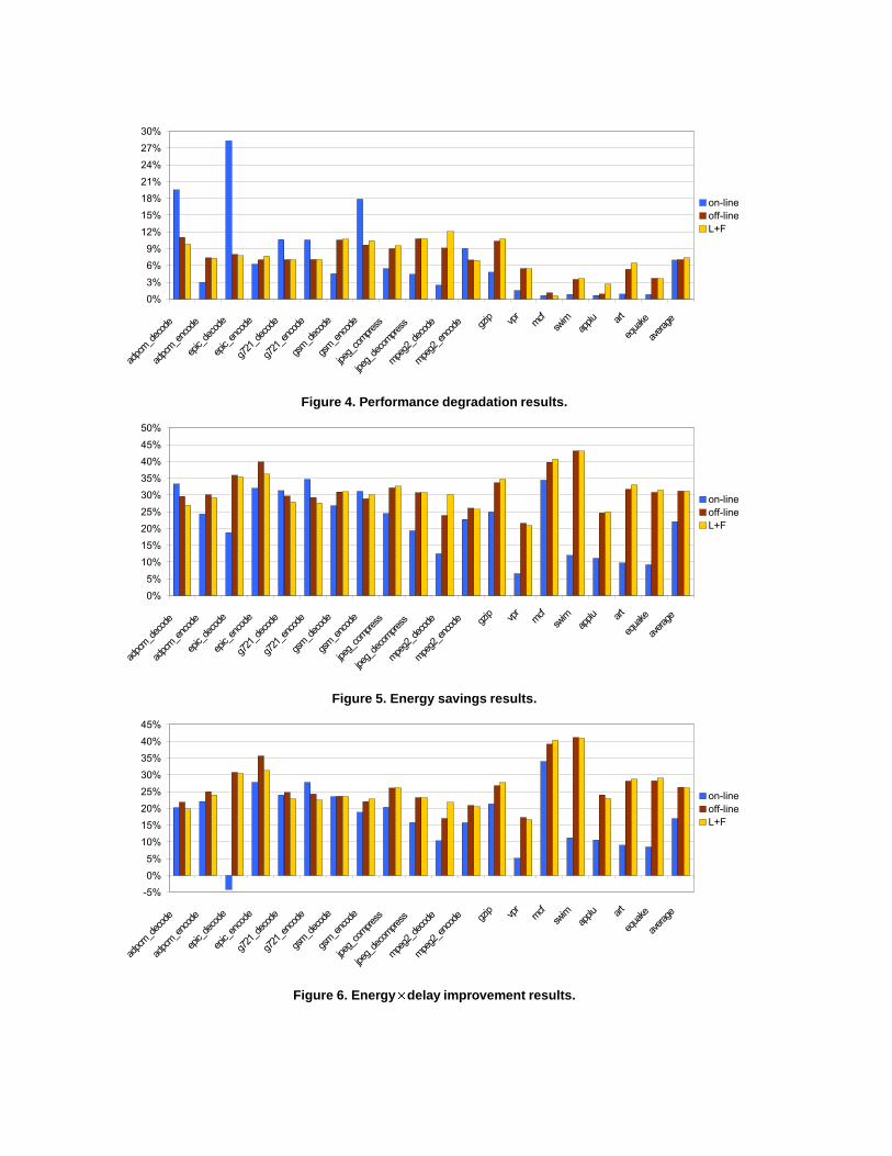
Figure 4. Performance degradation results.

Figure 5. Energy savings results.

Figure 6. Energy � delay improvement results.

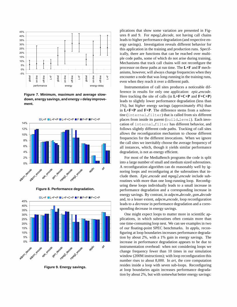
Figure 7. Minimum, maximum and average slow-down, energy savings, and energy � delayimprove-ment.

Figure 8. Performance degradation.

Figure 9. Energy savings.

plications that show some variation are presented in Fig-ures 8 and 9. For mpeg2 decode, not having call chainsleads to higher performance degradation (and respective en-ergy savings). Investigation reveals different behavior forthis application in the training and production runs. Specif-ically, there are functions that can be reached over multi-ple code paths, some of which do not arise during training.Mechanisms that track call chains will not reconfigure theprocessor on these paths at run time. The L+F and F mech-anisms, however, will always change frequencies when theyencounter a node that was long-running in the training runs,even when they reach it over a different path.

Instrumentation of call sites produces a noticeable dif-ference in results for only one application: epic encode.Here tracking the site of calls (in L+F+C+P and F+C+P)leads to slightly lower performance degradation (less than1%), but higher energy savings (approximately 4%) thanin L+F+P and F+P. The difference stems from a subrou-tine (internal filter) that is called from six differentplaces from inside its parent (build level). Each invo-cation of internal filter has different behavior, andfollows slightly different code paths. Tracking of call sitesallows the reconfiguration mechanism to choose differentfrequencies for the different invocations. When we ignorethe call sites we inevitably choose the average frequency ofall instances, which, though it yields similar performancedegradation, is not as energy efficient.

For most of the MediaBench programs the code is splitinto a large number of small and medium sized subroutines.A reconfiguration algorithm can do reasonably well by ig-noring loops and reconfiguring at the subroutines that in-clude them. Epic encode and mpeg2 encode include sub-routines with more than one long-running loop. Reconfig-uring these loops individually leads to a small increase inperformance degradation and a corresponding increase inenergy savings. By contrast, in adpcm decode, gsm decodeand, to a lesser extent, adpcm encode, loop reconfigurationleads to a decrease in performance degradation and a corre-sponding decrease in energy savings.

One might expect loops to matter more in scientific ap-plications, in which subroutines often contain more thanone time-consuming loop nest. We can see examples in twoof our floating-point SPEC benchmarks. In applu, recon-figuring at loop boundaries increases performance degrada-tion by about 2%, with a 1% gain in energy savings. Theincrease in performance degradation appears to be due toinstrumentation overhead: when not considering loops wechange frequency fewer than 10 times in our simulationwindow (200M instructions); with loop reconfiguration thisnumber rises to about 8,000. In art, the core computationresides inside a loop with seven sub-loops. Reconfiguringat loop boundaries again increases performance degrada-tion by about 2%, but with somewhat better energy savings:

roughly 5%.Based on these results, we recommend the L+F method,

i.e., reconfiguring at loop and function boundaries, but with-out including call chain information in the program state.It produces energy and performance results comparable tothose of the more complicated algorithms, with lower in-strumentation overhead. Using call chains as part of theprogram state may be a more appropriate method when ap-plication behavior changes significantly between the train-ing and production runs, but this situation does not arise inour application suite.

4.3. Sensitivity to Slowdown Threshold

Figures 10 and 11 show the energy savings andenergy � delay improvement achieved by the on-line, off-line and L+F algorithms relative to achieved slowdown.Several things are apparent from these figures. First, profile-based reconfiguration achieves almost the same energy sav-ings for equivalent performance degradation as the off-linealgorithm. The on-line algorithm on the other hand, al-though it is close to the off-line at low performance degra-dation targets, starts to tail off with increased slowdown.Beyond a slowdown of 8% the on-line algorithm continuesto save energy, but its energy � delay improvement stays thesame. Beyond about 15% (not shown here), energy � delayimprovement actually begins to decrease. By contrast, theoff-line and profile-based reconfiguration methods show amuch more linear relationship between performance degra-dation and energy � delay. We would expect it to tail offeventually, but much farther out on the curve.

4.4. Instrumentation Overhead

Table 3 shows the number of long-running nodes iden-tified by our profiling tool, as well as the total number ofnodes in the call tree, for both the data sets, under the mostaggressive (L+F+C+P) definition of calling context. It in-dicates the extent to which code paths identified in trainingruns match those that appear in production runs. (Our pro-filing mechanism, of course, does not construct call treesfor production runs. The numbers in Tables 3 and 4 werecollected for comparison purposes only.) The numbers inthe “Common” column indicate the number of tree nodes(long-running and total) that appear (with the same ances-tors) in the trees of both the training and reference sets. Thelast column (“Coverage”) presents these same numbers asa fraction of the number of nodes in the tree for the refer-ence set. It is clear from this column that the training andreference sets run most applications through the same codepaths. The notable exception is mpeg2 decode, in whichthe training set produces only 63% of the tree nodes pro-duced by the reference set. Moreover only 57% of thelong-running nodes identified under the training input setare the same as those identified under the reference input

0

5

10

15

20

25

30

35

40

45

0 2 4 6 8 10 12 14

Ene

rgy

Sav

ings

(%

)

Slowdown (%)

on-lineoff-line

L+F

Figure 10. Energy savings for the on-line, off-lineand L+F algorithms.

0

5

10

15

20

25

30

35

0 2 4 6 8 10 12 14

Ene

rgy-

Del

ay Im

prov

emen

t (%

)

Slowdown (%)

on-lineoff-line

L+F

Figure 11. Energy � delay improvement for the on-line, off-line and L+F algorithms.

set. When run with the reference input set, swim also pro-duces more reconfiguration points, because some loops inthe code run for more iterations and thus are classified aslong running. Unlike mpeg2 decode though, all reconfigu-ration points found with the training set are also found withthe reference set.

Table 4 addresses the cost of instrumentation, again forL+F+C+P. The second column (“Static”) shows the num-ber of static reconfiguration and instrumentation points inthe code. These numbers are in some cases smaller thanthe corresponding numbers in Table 3 because a subrou-tine or loop may correspond to multiple nodes in the calltree. Numbers are identical between the training and refer-ence data sets, again with the exception of mpeg2 decode.The third column of the table (“Dynamic”) shows howmany times we executed reconfiguration and instrumenta-tion code at run time (profiling with the training set andrunning with the reference set). These numbers are gen-erally much higher than the static ones, since we executeeach subroutine or loop many times. The only exception is

Benchmark TRAIN REF Common Coverageadpcm decode 2 4 2 4 2 4 1.00 1.00adpcm encode 2 4 2 4 2 4 1.00 1.00epic decode 18 25 18 25 18 25 1.00 1.00epic encode 65 91 65 91 65 91 1.00 1.00g721 decode 1 1 1 1 1 1 1.00 1.00g721 encode 1 1 1 1 1 1 1.00 1.00gsm decode 3 5 3 5 3 5 1.00 1.00gsm encode 6 9 6 9 6 9 1.00 1.00jpeg compress 11 17 11 17 11 17 1.00 1.00jpeg decompress 4 6 4 6 4 6 1.00 1.00mpeg2 decode 11 15 14 19 8 12 0.57 0.63mpeg2 encode 30 40 30 40 30 40 1.00 1.00gzip 78 224 70 196 65 182 0.93 0.93vpr 67 92 84 119 7 12 0.08 0.10mcf 26 41 26 41 26 41 1.00 1.00swim 16 23 25 32 16 23 0.64 0.78applu 61 77 68 85 60 77 0.98 0.91art 65 98 68 100 65 98 0.96 0.98equake 30 35 30 35 30 35 1.00 1.00

Table 3. Number of reconfiguration nodes and totalnumber of nodes in the call tree when profiling withthe reference and training sets.

Benchmark Static Dynamic Overheadadpcm decode 2 4 470 939 0.33%adpcm encode 2 4 470 939 0.17%epic decode 18 25 106 149 0.03%epic encode 27 40 4270 4441 0.29%g721 decode 1 1 1 1 0.00%g721 encode 1 1 1 1 0.00%gsm decode 3 5 5841 11681 0.30%gsm encode 6 9 12057 16579 0.35%jpeg compress 7 11 40 45 0.00%jpeg decompress 4 6 1411 1415 0.17%mpeg2 decode 4 7 1 2 0.00%mpeg2 encode 30 40 7264 7283 0.18%gzip 19 56 153 170 0.00%vpr 56 75 3303 3307 0.03%mcf 24 37 10477 16030 0.03%swim 16 23 5344 5352 0.03%applu 49 62 7968 7968 0.06%art 43 64 63080 65984 0.39%equake 30 35 34 41 0.00%

Table 4. Static and dynamic reconfiguration andinstrumentation points, and estimated run-timeoverhead for L+F+C+P.

mpeg2 decode, where the number of dynamic reconfigura-tion/instrumentation points is smaller than the static. Thishappens because we use ATOM to profile the applicationand so the static numbers correspond to the whole programexecution. The production runs, however, are executed onSimpleScalar, and use an instruction window of only 200Minstructions—much less than the entire program.

The final column of Table 4 shows the cost, as a percent-age of total application run time, of the extra instructionsinjected in the binary, as estimated by our simulator. These

Figure 12. Number of static reconfiguration and in-strumentation points and run-time overhead com-pared to L+F+C+P.

numbers, of course, are for the L+F+C+P worst case. Fig-ure 12 shows the number of instrumentation points, and as-sociated run-time overhead, of the simpler alternatives, nor-malized to the overhead of L+F+C+P. The first two sets ofbars compare the number of static reconfiguration and in-strumentation points in the code for the different profilingalgorithms, averaged across all applications. The L+F andF methods, of course, have no static instrumentation points,only reconfiguration points. Note also that the number ofstatic instrumentation points is independent of whether wetrack call chain information at run time; all that varies isthe cost of those instrumentation points. Thus, for example,L+F+P will always have the same number of long-runningsubroutines and loops as L+F. The last set of bars in Fig-ure 12 compares the run-time overhead of the different pro-filing methods. As expected, L+F+C+P has the highestoverhead. Interestingly, the number of instrumentation in-structions for L+F and F is so small that there is almostperfect scheduling with the rest of the program instructions,and the overhead is virtually zero.

Tables 3 and 4 also allow us to estimate the size of ourlookup tables. In the worst case (gzip) we need a )*),+-�.+0/ -entry table to keep track of the current node, and a )*),+ -entrytable to store all the domain frequencies: a total of about13KB. All other benchmarks need less than 4KB.

5. Related Work

Microprocessor manufacturers such as Intel [25] andTransmeta [18] offer processors capable of global dynamicfrequency and voltage scaling. Marculescu [26] and Hsuet al. [20] evaluated the use of whole-chip dynamic volt-age scaling (DVS) with minimal loss of performance usingcache misses as the trigger. Following the lead of Weiser etal. [32], many groups have proposed OS-level mechanismsto “squeeze out the idle time” in underloaded systems viawhole-chip DVS. Childers et al. [10] propose to trade IPCfor clock frequency, to achieve a user-requested quality ofservice from the system (expressed in MIPS). Processes

that can achieve higher MIPS than the current QoS settingare slowed to reduce energy consumption. By contrast, ourwork aims to stay as close as possible to the maximum per-formance of each individual application.

Other work [7, 28] proposes to steer instructions topipelines or functional units running statically at differentspeeds so as to exploit scheduling slack in the program tosave energy. Fields et al. [15] use a dependence graph simi-lar to ours, but constructed on the fly, to identify the criticalpath of an application. Their goal is to improve instruc-tion steering in clustered architectures and to improve valueprediction by selectively applying it to critical instructionsonly. Fields et al. [14] also introduce an on-line “slack” pre-dictor, based on the application’s recent history, in order tosteer instructions between a fast and a slow pipeline.

Huang et al. [21] also use profiling to reduce energy, butthey do not consider dynamic voltage and frequency scal-ing. Their profiler runs every important function with everycombination of four different power-saving techniques tosee which combination uses the least energy with negligi-ble slowdown. Our work minimizes performance degrada-tion by scaling only the portions of the processor that arenot on the critical path. We also consider reconfigurationbased on loop and call chain information, and require onlya single profiling run for each set of training data.

Several groups have used basic block or edge profil-ing and heuristics to identify heavily executed programpaths [8, 12, 16, 33]. Ball and Larus [3] first introducedan efficient technique for path profiling. In a follow-upstudy, Ammons et al. [1] describe a technique for contextsensitive profiling, introducing the notion of a calling con-text tree (CCT), on which our call trees are based. Am-mons et al. also describe a mechanism to construct the CCT,and to associate runtime statistics with tree nodes. Theydemonstrate that context sensitive profiling can expose dif-ferent behavior for functions called in different contexts.We borrow heavily from this work, extending it to includeloops as nodes of the CCT, and differentiating among callsto the same routine from different places within a singlecaller. The reason we need the CCT is also different inour case. Instead of the most frequently executed paths, weneed the minimum number of large-enough calling contextsthat cover the whole execution of the program.

6. Conclusions

We have described and evaluated a profile-driven recon-figuration mechanism for a Multiple Clock Domain micro-processor. Using data obtained during profiling runs, wemodify applications to scale frequencies and voltages at ap-propriate points during later production runs. Our resultssuggest that this mechanism provides a practical and effec-tive way to save significant amounts of energy in many ap-plications, with acceptable performance degradation.

In comparison to a baseline MCD processor, we demon-strate average energy savings of approximately 31%, withperformance degradation of 7%, on 19 multimedia andSPEC benchmarks. These results rival those obtained byan off-line analysis tool with perfect future knowledge, andare significantly better than those obtained using a previ-ously published hardware-based on-line reconfiguration al-gorithm. Our results also indicate that profile-driven recon-figuration is significantly more stable than the on-line alter-native. The downside is the need for training runs, whichmay be infeasible in some environments.

We believe that profile-driven application editing can beused for additional forms of architectural adaptation, e.g.the reconfiguration of CAM/RAM structures [2, 6]. We alsohope to develop our profiling and simulation infrastructureinto a general-purpose system for context-sensitive analysisof application performance and energy use.

Acknowledgements

We are grateful to Sandhya Dwarkadas for her many con-tributions to the MCD design and suggestions on this study.

References

[1] G. Ammons, T. Ball, and J. R. Larus. Exploiting HardwarePerformance Counters with Flow and Context Sensitive Pro-filing. In Proceedings of the 1997 ACM SIGPLAN Confer-ence on Programming Language Design and Implementa-tion, pages 85–96, June 1997.

[2] R. Balasubramonian, D. H. Albonesi, A. Buyuktosunoglu,and S. Dwarkadas. Memory Hierarchy Reconfiguration forEnergy and Performance in General-Purpose Processor Ar-chitectures. In Proceedings of the 33rd Annual IEEE/ACMInternational Symposium on Microarchitecture, pages 245–257, Dec. 2000.

[3] T. Ball and J. R. Larus. Efficient Path Profiling. In Pro-ceedings of the 29th Annual IEEE/ACM International Sym-posium on Microarchitecture, pages 46–57, Dec. 1996.

[4] D. Brooks, V. Tiwari, and M. Martonosi. Wattch: A Frame-work for Architectural-Level Power Analysis and Optimiza-tions. In Proceedings of the 27th International Symposiumon Computer Architecture, June 2000.

[5] D. Burger and T. Austin. The SimpleScalar Tool Set, Version2.0. Technical Report CS-TR-97-1342, Computer ScienceDepartment, University of Wisconsin, June 1997.

[6] A. Buyuktosunoglu, S. Schuster, D. Brooks, P. Bose,P. Cook, and D. H. Albonesi. An Adaptive Issue Queue forReduced Power at High Performance. In Proceedings of theWorkshop on Power-Aware Computer Systems, in conjunc-tion with ASPLOS-IX, Nov. 2000.

[7] J. Casmira and D. Grunwald. Dynamic Instruction Schedul-ing Slack. In Proceedings of the Kool Chips Workshop, inconjunction with MICRO-33, Dec. 2000.

[8] P. P. Chang. Trace Selection for Compiling Large C Appli-cation Programs to Microcode. In Proceedings of the 21stAnnual Workshop on Microprogramming and Microarchi-tecture (MICRO 21), pages 21–29, Nov. 1988.

[9] D. M. Chapiro. Globally Asynchronous Locally Syn-chronous Systems. PhD thesis, Stanford University, 1984.

[10] B. R. Childers, H. Tang, and R. Melhem. Adapting Proces-sor Supply Voltage to Instruction-Level Parallelism. In Pro-ceedings of the Kool Chips Workshop, in conjunction withMICRO-34, Dec. 2001.

[11] L. T. Clark. Circuit Design of XScale 132 Microprocessors.In 2001 Symposium on VLSI Circuits, Short Course on Phys-ical Design for Low-Power and High-Performance Micro-processor Circuits, June 2001.

[12] J. R. Ellis. A Compiler for VLIW Architectures. TechnicalReport YALEU/DCS/RR-364, Yale University, Departmentof Computer Science, Feb. 1985.

[13] A. Eustace and A. Srivastava. ATOM: A Flexible Interfacefor Building High Performance Program Analysis Tools.In Proceedings of the USENIX 1995 Technical Conference,Jan. 1995.

[14] B. Fields, R. Bodı́k, and M. D. Hill. Slack: Maximizing Per-formance Under Technological Constraints. In Proceedingsof the 29th International Symposium on Computer Architec-ture, pages 47–58, May 2002.

[15] B. Fields, S. Rubin, and R. Bodı́k. Focusing Processor Poli-cies via Critical-Path Prediction. In Proceedings of the 28thInternational Symposium on Computer Architecture, July2001.

[16] J. A. Fisher. Trace Scheduling: A Technique for GlobalMicrocode Compaction. IEEE Transactions on Computers,30(7):478–490, July 1981.

[17] M. Fleischmann. Crusoe Power Management – Reducingthe Operating Power with LongRun. In Proceedings of theHOT CHIPS Symposium XII, Aug. 2000.

[18] T. R. Halfhill. Transmeta breaks x86 low power barrier. Mi-croprocessor Report, 14(2), Feb. 2000.

[19] J. L. Henning. SPEC CPU2000: Measuring CPU Perfor-mance in the New Millennium. Computer, pages 28–35,July 2000.

[20] C.-H. Hsu, U. Kremer, and M. Hsiao. Compiler-DirectedDynamic Frequency and Voltage Scaling. In Proceedings ofthe Workshop on Power-Aware Computer Systems, in con-junction with ASPLOS-IX, Nov. 2000.

[21] M. Huang, J. Renau, and J. Torrellas. Profile-Based EnergyReduction in High-Performance Processors. In Proceedingsof the 4th Workshop on Feedback-Directed and DynamicOptimization (FDDO-4), Dec. 2001.

[22] G. C. Hunt and M. L. Scott. The Coign Automatic Dis-tributed Partitioning System. In Proceedings of the 3rdUSENIX Symposium on Operating Systems Design and Im-plementation, Feb. 1999.

[23] A. Iyer and D. Marculescu. Power and Performance Evalu-ation of Globally Asynchronous Locally Synchronous Pro-cessors. In Proceedings of the 29th International Symposiumon Computer Architecture, May 2002.

[24] C. Lee, M. Potkonjak, and W. H. Mangione-Smith. Media-bench: a Tool for Evaluating and Synthesizing Multimediaand Communications Systems. In Proceedings of the 30thAnnual IEEE/ACM International Symposium on Microar-chitecture, pages 330–335, Dec. 1997.

[25] S. Leibson. XScale (StrongArm-2) Muscles In. Micropro-cessor Report, 14(9):7–12, Sept. 2000.

[26] D. Marculescu. On the Use of Microarchitecture-Driven Dy-namic Voltage Scaling. In Proceedings of the Workshop onComplexity-Effective Design, in conjunction with ISCA-27,June 2000.

[27] Intel Corp. Datasheet: Intel R4

Pentium R4

4 Processor with512-KB L2 cache on 0.13 Micron Process at 2 GHz–3.06GHz. Available at http://www.intel.com/design/pentium4/-datashts/298643.htm, Nov. 2002.

[28] R. Pyreddy and G. Tyson. Evaluating Design Tradeoffs inDual Speed Pipelines. In Proceedings of the Workshop onComplexity-Effective Design, in conjunction with ISCA-28,June 2001.

[29] G. Semeraro, D. H. Albonesi, S. G. Dropsho, G. Magklis,S. Dwarkadas, and M. L. Scott. Dynamic Frequency andVoltage Control for a Multiple Clock Domain Microarchi-tecture. In Proceedings of the 35th Annual IEEE/ACM In-ternational Symposium on Microarchitecture, Nov. 2002.

[30] G. Semeraro, G. Magklis, R. Balasubramonian, D. H. Al-bonesi, S. Dwarkadas, and M. L. Scott. Energy-EfficientProcessor Design Using Multiple Clock Domains with Dy-namic Voltage and Frequency Scaling. In Proceedings of the8th International Symposium on High-Performance Com-puter Architecture, Feb. 2002.

[31] A. E. Sjogren and C. J. Myers. Interfacing Synchronous andAsynchronous Modules Within A High-Speed Pipeline. InProceedings of the 17th Conference on Advanced Researchin VLSI, pages 47–61, Sept. 1997.

[32] M. Weiser, A. Demers, B. Welch, and S. Shenker. Schedul-ing for Reduced CPU Energy. In Proceedings of the 1stUSENIX Symposium on Operating Systems Design and Im-plementation, Nov. 1994.

[33] C. Young and M. D. Smith. Improving the Accuracy ofStatic Branch Prediction Using Branch Correlation. In Pro-ceedings of the 6th International Conference on Architec-tural Support for Programming Languages and OperatingSystems, pages 232–241, Oct. 1994.