reliability assessment of drag embedment anchors and
TRANSCRIPT

Reliability Assessment of Drag Embedment Anchors
and Laterally Loaded Buried Pipelines
by
© Amin Aslkhalili
A thesis submitted to the
School of Graduate Studies
In partial fulfillment of the requirements for the degree of
Master of Engineering
Faculty of Engineering and Applied Science
Memorial University of Newfoundland
October 2020
St. John’s, Newfoundland
i
Abstract
Drag embedment anchors and buried subsea pipelines are two important elements of the offshore
field developments that are used for station-keeping of floating facilities and transferring the
hydrocarbons, respectively. The lateral soil resistance against the drag anchors and pipelines are
mobilized in a similar fashion with identical conventional design equations. This is fundamentally
caused by similar lateral projection of the anchor and pipe geometries. The reliability assessment
of the drag embedment anchors as a key component of mooring systems, and the lateral response
of trenched pipelines as crucial structural elements are significantly important due to a range of
uncertainties involved in the design process. Despite the similar design equations for lateral soil
resistance against the moving anchor and pipe, these elements are subjected to different kinds of
loadings and uncertainties that are expected to affect their reliability indices. In this study, the
reliability of drag embedment anchors and laterally displaced pipelines were conducted and
compared to investigate the extent of similar fashions in the lateral response of these two elements
to large displacements. Both uniform and non-homogeneous soil domains were considered and
compared to evaluate the impact of more realistic design scenarios. Macro spreadsheets were
developed for iterative limit state and kinematic analyses and obtaining the holding capacity of
drag embedment anchors. The lateral force-displacement responses of the buried pipelines were
extracted from published centrifuge model tests and incorporated into finite element models in
ABAQUS. Automation Python scripts were developed to perform a comprehensive series of
numerical analyses and post-process the outputs to construct the required databases. Response
surfaces were developed and probabilistic analyses were conducted by using the first order
reliability method (FORM) to obtain the reliability indices and failure probabilities.
ii
Comparative studies were conducted to obtain an equivalent annual probability of failure between
the pipelines and drag anchors. The study showed that the similar conventional approaches for
modeling of the anchors and pipelines lateral displacement might be acceptable for homogeneous
soil domains. However, the reliability indices were significantly affected by defining non-
homogenous soil domains. It was observed that the magnitude of the reliability indices in the
layered soil strata and trenched/backfilled conditions could be significantly reduced. This, in turn,
revealed the need for improving the current design codes to incorporate more realistic conditions.
The proposed probabilistic approach was found robust to optimize the subsea configuration of the
anchors and pipelines and improve the reliability indices. The study revealed several important
trends in anchors and pipeline-seabed interactions and provided an in-depth insight into its impact
on reliability assessment and a safe and cost-effective design.

iii
Acknowledgment
First of all, I would like to thank my supervisor, Dr. Hodjat Shiri, for his valuable guidance,
supports, and the belief that he had in me to allow me to be a part of his research team. He was
beside me in every step of this journey, and I would never forget what he had taught me.
My best regards go to Dr. Sohrab Zendehboudi, my co-supervisor, who helped me through this
path.
I want to gratefully acknowledge the financial support of this research by Wood PLC via
establishing the Wood Group Chair in Arctic and harsh environment engineering at Memorial
University, the NL Tourism, Culture, Industry and Innovation (TCII) via CRD collaborative
funding program, the Natural Sciences and Engineering Research Council of Canada (NSERC)
via Engage funding program, the in-kind technical supports and advice of TechnipFMC, NL,
Canada, the Memorial University of Newfoundland through VP start-up fund, and the school of
graduate studies (SGS) baseline fund.
Last but foremost, my sincere thanks go to my Mother, Father, and beloved wife (Setareh). They
lovingly encouraged me through my studies and supported me emotionally in every day of this
stressful journey. I am thankful for having you beside me.
iv
Contents
Abstract ................................................................................................................................... i
Acknowledgment ................................................................................................................. iii
Contents ................................................................................................................................ iv
List of Figures ...................................................................................................................... vii
List of Tables ........................................................................................................................ ix
List of Symbols and Abbreviations ..................................................................................... x
Chapter 1. Introduction ................................................................................................... 1
1.1 Background and Motivation ........................................................................................ 1
1.1.1 Drag Embedment Anchors .............................................................................. 1
1.1.2 Subsea Pipelines.............................................................................................. 3
1.2 Research Objectives .................................................................................................... 4
1.3 Thesis Organization..................................................................................................... 5
Chapter 2. Literature Review ......................................................................................... 7
2.1 Mooring and Anchoring System ................................................................................. 7
2.1.1 Drag Anchor Behaviors ................................................................................ 10
2.1.2 Anchor Chain ................................................................................................ 11
2.1.3 Theoretical Anchor Models .......................................................................... 11
2.2 Buried Subsea Pipelines ............................................................................................ 14
2.3 Lateral Pipeline Soil Interaction ................................................................................ 15
2.4 Reliability Assessment .............................................................................................. 16
2.5 Reliability Analysis Methods .................................................................................... 17
2.5.1 First Order Reliability Method (FORM)....................................................... 18
2.5.2 Response Surface Method............................................................................. 20
Chapter 3. Reliability Assessment of Drag Embedment Anchors in Sand for Catenary
Mooring Systems ............................................................................................................ 22
Abstract ............................................................................................................................ 23
3.1 Introduction ............................................................................................................... 24
3.2 Methodology ............................................................................................................. 26
3.3 Modeling Drag Embedment Anchor ......................................................................... 27
3.4 Soil-Chain Interaction ............................................................................................... 27
3.5 Anchor Holding Capacity.......................................................................................... 31
3.6 Anchor Kinematics .................................................................................................... 33
v
3.7 Developing Iterative Macro for Prediction of Anchor Performance ......................... 34
3.8 Anchors Used in the Current Study........................................................................... 36
3.9 Finite Element Mooring Analysis ............................................................................. 38
3.10 Reliability Analysis ................................................................................................ 40
3.11 Limit State Function ............................................................................................... 40
3.12 Probabilistic Modelling of Anchor Capacity .......................................................... 42
3.13 Probabilistic Modelling of Line Tension ................................................................ 45
3.14 Results of Reliability Analysis ............................................................................... 47
3.15 Equivalent Reliability Study in Sand and Clay ...................................................... 51
3.16 Conclusions ............................................................................................................. 52
Acknowledgments ............................................................................................................ 54
References ........................................................................................................................ 55
Chapter 4. Reliability Assessment of Drag Embedment Anchors in Layered Seabed,
Clay over Sand ................................................................................................................ 59
Abstract ............................................................................................................................ 60
4.1 Introduction ............................................................................................................... 62
4.2 Methodology ............................................................................................................. 64
4.3 Modeling Drag Anchor in Layered Soil .................................................................... 65
4.3.1 Chain-Soil frictional capacity ....................................................................... 65
4.3.2 Anchor Holding Capacity ............................................................................. 68
4.3.3 Developing Calculation Spreadsheet ............................................................ 71
4.3.4 Anchors Selected for Reliability Studies ...................................................... 74
4.4 Finite Element Mooring Analysis ............................................................................. 76
4.5 Reliability Analysis ................................................................................................... 77
4.5.1 Limit State Function ..................................................................................... 77
4.5.2 Probabilistic Modelling of Anchor Capacity ................................................ 79
4.5.3 Probabilistic Model of Line Tension ............................................................ 82
4.5.4 Results of Reliability Analysis...................................................................... 85
4.5.5 Comparison Between the Reliability of Anchors in Homogenous and Layered
Soils............................................................................................................... 89
4.6 Conclusion ................................................................................................................. 90
Acknowledgments ............................................................................................................ 92
References ........................................................................................................................ 93
Chapter 5. Probabilistic Assessment of Lateral Pipeline-Backfill-Trench Interaction
………………………………………………………………………………96
Abstract ............................................................................................................................ 97
vi
5.1 Introduction ............................................................................................................... 98
5.2 Finite Element Model .............................................................................................. 100
5.2.1 Pipe-Soil Model .......................................................................................... 101
5.2.2 Pipe Properties ............................................................................................ 102
5.3 Probabilistic Model ................................................................................................. 103
5.3.1 Limit State Criteria ..................................................................................... 105
5.3.2 Probabilistic Characterization of Seismic Hazard ...................................... 106
5.3.3 Probabilistic Fragility of the Pipeline ......................................................... 106
5.3.4 Probabilistic Characterization of Soil and Trench ...................................... 108
5.3.5 Iterative Procedure ...................................................................................... 109
5.4 Results and Discussion ............................................................................................ 114
5.5 Conclusions and Recommendations........................................................................ 118
Acknowledgment ............................................................................................................ 119
References ...................................................................................................................... 120
Chapter 6. Summary, Conclusions and recommendations ...................................... 125
6.1 Drag Embedment Anchor-Seabed Interaction ........................................................ 125
6.2 Lateral Pipeline-Backfill-Trench Interaction .......................................................... 127
6.3 Comparative Reliability of Drag Embedment Anchor and Buried Pipelines ......... 128
6.4 Recommendations for Future Studies ..................................................................... 129
References .......................................................................................................................... 131
vii
List of Figures
Figure 2-1. Different offshore structures .................................................................................. 7
Figure 2-2. Different mooring system ...................................................................................... 8
Figure 2-3. The typical arrangement of drag anchor and chain .............................................. 10
Figure 2-4. Buried pipeline subjected to ground movement ................................................... 15
Figure 2-5. The graphical interpretation of the reliability index and three steps for the FORM
calculation method ................................................................................................ 20
Figure 3-1. Detail of drag embedment anchor in the catenary mooring system ..................... 24
Figure 3-2. Force equilibrium of chain element ..................................................................... 28
Figure 3-3. Comparison of chain profile in sand .................................................................... 31
Figure 3-4. The three-dimensional failure wedge in plan and side view and force system of the
anchor .................................................................................................................... 32
Figure 3-5. Analysis flow chart for embedment history of drag anchors ............................... 35
Figure 3-6. Comparison of results for anchor efficiency ........................................................ 35
Figure 3-7. Comparison of results for anchor holding capacity ............................................. 36
Figure 3-8. Schematic of the modeled anchor in the present study ........................................ 37
Figure 3-9. Schematic plan view of the mooring line arrangement ........................................ 39
Figure 3-10. Generic semisubmersible RAO, the head sea .................................................... 39
Figure 3-11. Histograms of simulated and fitted capacities at mudline, (a) absolute frequency,
(b) Cumulative frequency ..................................................................................... 43
Figure 3-12. The mean and standard deviation of anchor capacity versus fluke length; MK6
............................................................................................................................... 45
Figure 3-13. Response surfaces for Tmean and Tdyn, max ........................................................... 46
Figure 3-14. Annual reliability index versus (a) fluke length, and (b) anchor weight............ 48
Figure 3-15. The logarithm of failure probability versus (a) fluke length, and (b) anchor weight
............................................................................................................................... 50
Figure 3-16. Equivalent anchor class (weight) comparison between sand & clay ................. 52
Figure 4-1. Drag embedment anchor configuration with a catenary mooring line ................. 62
Figure 4-2. Force equilibrium of the chain element ............................................................... 66
Figure 4-3. Embedded chain load behavior in clay over sand layered soil ............................ 68
Figure 4-4. Force system of anchor-soil in clay over sand ..................................................... 69
Figure 4-5. Flowchart of anchor embedment calculation in the layered seabed .................... 72
viii
Figure 4-6. Comparison between anchor efficiency results .................................................... 74
Figure 4-7. Schematic plan and side view of the modeled anchor in the present study ......... 75
Figure 4-8. Generic semisubmersible RAO, the head sea ...................................................... 76
Figure 4-9. Histograms of simulated capacities at mudline, (a) absolute frequency, (b)
cumulative frequency ............................................................................................ 80
Figure 4-10. The mean and standard deviation of anchor capacity against fluke length for MK6
............................................................................................................................... 82
Figure 4-11. Response surfaces of Tmean and Tdyn, max ..................................................... 84
Figure 4-12. Annual reliability index versus (a) fluke length, and (b) anchor weight............ 86
Figure 4-13. The logarithm of failure probability versus (a) fluke length, and (b) anchor weight
............................................................................................................................... 88
Figure 4-14. Annular reliability index versus anchor weight (a) MK5, (b) MK6 .................. 90
Figure 5-1. Schematic illustration of the trenched buried pipeline subjected to a strike-slip fault
............................................................................................................................... 98
Figure 5-2. Trenched buried pipe-soil interaction in a) continuum analysis, b) idealized
structural model, and c) soil load-displacement response curves in three directions
............................................................................................................................. 101
Figure 5-3. Flow chart of probabilistic analysis ................................................................... 110
Figure 5-4. The fitted distribution and histogram of maximum von Mises stress and
compressive strain for the trenched (a, b) and no trench pipe (c, d) ................... 111
Figure 5-5. Mean and Stdev of maximum von Mises stress (a, b) and compressive strain (c, d)
with the variation of trench/pipe depth ............................................................... 113
Figure 5-6. Mean and Stdev of maximum von Mises stress (a, b) and compressive strain (c, d)
with the variation trench width ........................................................................... 113
Figure 5-7. Logarithmic probability of exceedance for serviceability (left) and ultimate (right)
limit states with the variation of trench depth (a, b) and trench width (c, d) ...... 114
Figure 5-8. The logarithm of annual exceedance probability against trench depth and width for
serviceability (a, b) and ultimate limit states (c, d) ............................................. 116
ix
List of Tables
Table 3-1. Soil and anchor input parameters in the current analysis ...................................... 36
Table 3-2. Main dimensions for 12 t anchors (Vryhof Anchors, 2010) ................................. 37
Table 3-3. Properties of the modeled drag anchors ................................................................ 38
Table 3-4. Catenary mooring system characteristic ................................................................ 39
Table 3-5. Statistical properties of anchor capacity at pad -eye and mudline ......................... 44
Table 3-6. Distribution parameters of environmental variables ............................................. 47
Table 3-7. Estimated correlation coefficients ......................................................................... 47
Table 3-8. Equivalency map of anchor classes in sand and clay with a close reliability indices
............................................................................................................................... 52
Table 4-1. Soil and anchor input parameters in the current analysis ...................................... 73
Table 4-2. Main dimensions for 12 t anchors (Vryhof Anchors, 2010) ................................. 75
Table 4-3. Properties of the modeled drag anchors ................................................................ 76
Table 4-4. Characteristic of the catenary mooring system ..................................................... 77
Table 4-5. Statistical properties of anchor capacity at pad -eye and mudline ......................... 81
Table 4-6. Distribution parameters of environmental variables ............................................. 85
Table 4-7. Estimated correlation coefficients ......................................................................... 85
Table 5-1. Pipeline properties for the current analysis ......................................................... 103
Table 5-2. Strain limits characterization ............................................................................... 108
Table 5-3. The variation of trench geometry (depth and width) ........................................... 109
Table 5-4. Statistical properties (mean, ; standard deviation, ; coefficient of variation, ) of
Maximum compressive strain for trench geometry of (width = 2.631D, depth = 3D)
and Maximum von Mises stress for trench geometry of (width = 3.158D, depth =
1.842D) ............................................................................................................... 111
Table 5-5. The desired trench geometry for different design scenarios................................ 117
Table 6-1. Equivalency map of MK5 anchor with the buried pipeline ................................ 128
Table 6-2. Equivalency map of MK6 anchor with the buried pipeline ................................ 128

x
List of Symbols and Abbreviations
As Area of shank
At Fluke tip area
bc Effective chain width
bf Fluke width
bs Shank width
Cub Backfill soil undrained shear strength
Cun Native soil undrained shear strength
d Nominal chain diameter, Trench depth
D Pad-eye embedment depth, Pipe outer diameter
da Attachment depth
dai Initial fluke depth
daeff Effective attachment depth
dc Depth of overlaying clay layer
df Fluke thickness
ds Average depth of the shank
dt Depth of fluke’s tip
dsb Embedment depth of back lower point of shank
dsf Embedment depth of front lower point of shank
dua The absolute displacement of the anchor
dus Soil wedge displacement
dusa Displacement of the soil relative to the anchor
dw Wave direction
dwc Current direction relative to wave
dww Wind direction relative to wave
En Normal circumference parameter
En Tangential circumference parameter
F Form factor (Neubecker and Randolph 1996)
fy Yield stress of pipe
𝑓(𝑋) Joint probability function of 𝑋
F Friction force
Ff The fluke force
Ffb The force on the back of the fluke
Ffc1 Normal fluke clay force
Ffc2 Shear fluke clay force
Ffs Sand fluke force
𝐹𝑅(𝑟) Cumulative distribution of load
Fs The shank force
𝐹𝑆(𝑠) Cumulative distribution of capacity
Fsc1 Normal shank clay force
Fsc2 Shear shank clay force
Fsc3 Side shank clay force
Fss Sand shank force
Ft Fluke tip force
𝐺(𝑋) Limit state function, Performance function
𝐺(𝑅, 𝑆) Limit state function
𝐺(𝑢𝑅, 𝑢𝑆) Transformed limit state function to standard normal space
𝐺′(𝑢𝑅 , 𝑢𝑆) Approximation of transformed limit state function
h Back edge of the fluke
H Depth of fluke tips
Hs Significant wave height
Lf Fluke length
Lf Caisson length (Silvia-Gonzalez et al. 2013)
Ls Shank length

xi
M Magnitude of the earthquake
Nc Bearing capacity factor of clay
Nq Standard bearing capacity factor and bearing capacity for sand
Nqs Shank bearing factor in sand
Nt Bearing factor of fluke tip in sand
pF Probability of failure
pFa Annual probability of failure
Pu1 First peak of lateral soil force per unit length of pipe
Pu2 Second peak of lateral soil force per unit length of pipe
ΔP1 Displacement at Pu1
ΔP2 Displacement at Pu2
q Bearing pressure
qsand Demonstrative of standard sand strength
Q Normal soil reaction on chain segment
Qd Peak of downward vertical soil force per length of pipe
Qeff Effective profile of resistance
Qu Peak of upward vertical soil force per length of pipe
Q̅ Average bearing resistance per unit length of chain over embedment depth
Δqd Displacement at Qd
Δqu Displacement at Qu
R Anchor capacity at mudline, Soil reaction
𝑅(𝑋) Load function
Ra Anchor capacity at pad-eye
Rd Design anchor capacity at mudline
Rd,a Design resistances at the pad-eye
ri Distance between point 𝑖 and anchor shackle
s Length of chain
sug Undrained shear strength gradient
su0 Surface undrained shear strength
𝑆(𝑋) Capacity function
SF Side friction
t Pipe thickness
T Line tension
Ta Line tension at the pad-eye
Ta Revised anchor capacity at the pad-eye
Td Design line tension at mudline
Td,a Design tensions at the pad-eye
Tdyn,max Mean maximum dynamic line tension
Tdyn,max-C Characteristic mean maximum dynamic tension
Tmean Mean line tension
Tmean-C Characteristic mean line tension
To Chain tension at mudline
Tp Spectral peak period
Tu Peak of axial soil force per length of pipe
T* Normalized tension
∆t Extreme sea state duration, Displacement at Tu
𝑢𝑅 Rosenblatt transformation of load
𝑢𝑆 Rosenblatt transformation of capacity
𝑢∗ Most probable point
U10 Wind velocity
Uc Surface current velocity direction
w, wc Chain self-weight per unit length, Trench width
Wa Anchor dry weight
Wa Sub anchor weight
Ws The mobilized soil mass
Wsc Weight of soil wedge

xii
xa Anchor horizontal displacement
X Absolute displacement of point 𝑖, Set of uncertain parameters, Probability density function
x* Horizontal distance normalised by D
∆x Absolute penetration increments of the origin
Y Absolute displacement of point 𝑖
∆y Absolute penetration increments of the origin
Z Depth below mudline
z* Depth normalised by D
αh Strain hardening parameter
αgw Girth weld factor
s Side shear factor
β Inclination of fluke, reliability index, The angle of pipe-fault intersection
βannual Annual reliability index
F First order reliability index
i Initial fluke angle
γ Clay soil unit weight
γ Resistance strain factor
γ Effective unit weight of soil
c Clay effective unit weight
γdyn Partial safety factor on dynamic line tension
γmean Partial safety factor on mean line tension
s Sand effective unit weight
Coefficient of variation
c Seabed surface depth
fs Average fault movement
c Compression strain
d Design compression strain
a Anchor efficiency
θ Line tension angle
θa Line tension angle at the pad-eye
θf Fluke wedge angle
θfs Fluke-shank angle
θi Polar coordinate angle of point 𝑖 θo Line tension angle at mudline
∆θ Rotation increments of the origin
λ Failure wedge angle, mean annual rate of extreme sea states, Occurrence rate
µ Chain-soil friction coefficient, Mean
h Hoop stress
∅′, ∅𝑝 Soil friction angle
∅𝑝 Sand peak friction angle
Θ Vector of environmental variables
ψ Dilation angle
−1( ) Inverse of the cumulative standard normal function
1
Chapter 1. Introduction
1.1 Background and Motivation
Offshore field developments require drag embedment anchors as a critical component of the
mooring system and buried subsea pipelines for station-keeping the floating structures, and
hydrocarbons transportation. Similar lateral projection of the anchor and pipe geometries results
in the similarity between the lateral soil resistance against the drag anchors and pipelines, which
are organized using conventional design equations (Dickin, 1994; Ng, 1994). The broad range of
uncertainties involved in the design process imposes the reliability assessment of crucial structural
elements such as the drag embedment anchors and the lateral response of trenched pipelines. These
structural elements encounter different types of loadings and uncertainties, which affect their
reliability indices. In the current study, the reliability of drag embedment anchors and laterally
displaced pipelines were explored and compared in both homogeneous and non-homogenous soil
to investigate the similarity extent of lateral response of these two elements under large
displacements. The following sections provide a brief introduction about the drag embedment
anchors and buried pipelines:
1.1.1 Drag Embedment Anchors
Floating facilities such as operation vessels, semi-submersibles, Spars, and FSPOs, etc. are used
to extraction and production of hydrocarbon from offshore reserves. The ideal solution for station
keeping of floating facilities is using catenary mooring systems combined with seabed anchors.
Different types of anchors could be used with mooring systems like suction anchors, pile anchors,
screw-in anchors, plate anchors, deadweight anchors, and drag embedment anchors. Nevertheless,
the drag embedment anchors are considered to be the most attractive method due to their cheap
and straightforward installation procedure and could be used for temporary and permanent
2
mooring systems. Despite convenient installation, the evaluation of holding capacity in drag
embedment anchors is challenging due to their complex geometry and uncertain interaction
between the seabed and anchors.
In order to have safe floating facilities and offshore environments, it is essential to fulfilling the
reliability of the mooring and anchoring system. This requirement has increased by expanding
offshore exploration and extraction toward the deep waters and harsh environments that need high
capacity anchors and high strength components in the mooring system. On the other hand, the
complex behavior of seabed with the anchor and environmental loads along with the unavailability
to inspect, maintain and, monitor of drag anchors highlights the importance of reliability
assessments to reduce the probability of failure in the system as much as possible.
The reliability assessment of drag embedment anchor families is dramatically less developed
compared to other anchor types, e.g., suction anchors. In the literature, there are numerous of
studies focused on the reliability assessment of various anchor types including suction anchors
(Choi, 2007; Valle-molina et al., 2008; Clukey et al., 2013; Silva-González et al., 2013; Montes-
Iturrizaga and Heredia-Zavoni, 2016; Rendón-Conde and Heredia-Zavoni, 2016). However, due
to complicated interaction between the seabed and anchors, limited access to holding capacity
databases, and the difficulties associated with performing computational analyses to estimate the
reliability of drag embedment anchor families. (Moharrami and Shiri, 2018) studied the reliability
of drag embedment anchors in clay, but there are no reliability investigations in the sand or layered
seabed. For estimation of holding capacity, there are some design codes (e.g., API RP 2SK, 2008)
which only recommend a unique procedure for homogenous (clay or sand) and layered seabed. In
the layered seabed, this simplification will dramatically affect the reliability of the system, and the
level of risk will not be appropriately estimated.
3
1.1.2 Subsea Pipelines
Buried pipelines considered as one of the most attractive ways for transportation of hydrocarbons
and other contents in onshore and offshore environments. In Canada, as stated by the Canadian
Energy Pipeline Association (CEPA), 130,000 km of underground transportation pipelines operate
daily to transmit 97 percent of Canada’s consumption of crude oil and natural gas from production
plants to markets across North America (www.cepa.com). Both offshore and onshore buried
pipelines pass through different types of soils where the integrity of pipes may be threatened by a
variety of subsea geohazards and the resulted ground movements, which could cause significant
damages and leading to their failure. European Gas pipeline Incident data Group (EGIG) stated
the fourth primary reason for pipeline failures is ground movements, and pipe rupture is the
consequence of almost half of these incidents (EGIG, 2005). Ground movements initiate relative
lateral movements between soil and pipe that may cause extra loading on the buried pipelines. In
designing subsea pipelines, understanding the behavior of buried pipelines under loading is an
important engineering consideration.
Trenching the buried pipelines is a known and common construction practice during the
installation of subsea pipes. Due to excavation or supplying the required soil inside the trench from
other areas with different geotechnical properties, the backfill material which fills the trench would
not have the same properties as the native trench soil has. Therefore, the soil around the buried
pipelines is not homogenous anymore and comprised of backfill and native soil, which have
different soil resistance against the pipe during different phases of pipe movement through the soil.
From the state of design point of view, the current design guidelines utilize discrete nonlinear
springs for each orthogonal loading axis (x, y, and z) for representing the soil resistance in the
axial, vertical and lateral direction on buried pipelines (ASCE, 1984; PRCI, 2009; ALA, 2005;
4
DNV, 2007). In the most design guidelines except PRCI (2009), the surrounding soil is assumed
to be homogenous and the effect of the trench is neglected. There are some studies in the literature
which covers the impact of the trench and backfill on the lateral interaction of soil-pipe in clay (C-
CORE, 2003; Phillips et al., 2004). The results of those studies are incorporated in the PRCI (2009)
design guideline, which could help to have a better understating and calculation of lateral force-
displacement relations in clay.
The geometry and the geotechnical properties of the backfill and native soil of the trench directly
affects the lateral force-displacement of trenched pipelines. Therefore, in order to have a safe and
cost-effective trenched pipeline design at the same time, it is required to perform reliability
analysis to find out the most optimum and reliable trench geometry and see the effect of using
guidelines which neglect consideration of trench effects against more advanced methodologies
(covering the trench effects) on the reliability of the system.
1.2 Research Objectives
The research objectives were set to fill some of the key knowledge gaps. These objectives were
successfully achieved throughout the study:
• Develop numerical and analytical models to obtain the holding capacity of anchors and the
dynamic mooring line tensions as the input parameters for the probabilistic modeling and
reliability assessment of drag embedment anchors in sand. There was no study in the
literature to have considered the sand seabed.
• Extend the developed reliability analysis model to study the effect of complex layered
seabed soil strata.
5
• Develop a three-dimensional finite element model integrated with a probabilistic model for
reliability assessment of the fault-induced lateral pipe/soil interaction in homogeneous
seabed stratum.
• Extend the developed model to capture the effect of trenching/backfilling on lateral pipe
response to the ground movement.
• Compare the reliabilities of the drag embedment anchors and the laterally displaced
pipelines with the effect of non-homogeneous seabed soil strata.
1.3 Thesis Organization
The thesis was prepared in a paper-based format. The outcomes are presented through six chapters.
Chapter 1 describes the background, motivation, objectives, and organization of the thesis. Chapter
2 includes a critical literature review. It is worth mentioning that each chapter is a manuscript and
has its independent literature review. However, to facilitate reading the thesis, the literature review
of various chapters were properly integrated and presented in Chapter 2. Chapter 3 presents a
journal paper published in “Safety in Extreme Environments” (Springer). The paper investigates
the reliability assessment of drag embedment anchors in sand that has never been done in the past.
Chapter 4 is a comprehensive conference paper accepted for oral presentation in the 73rd Canadian
Geotechnical Conference (GeoCalgary 2020). The paper presents the reliability assessment of drag
embedment anchors in complex layered seabed soil stratum. In this chapter, the reliability indices
of the anchors in layered seabed was compared with the sand seabed to investigate the effect of
non-homogeneous soil conditions. Chapter 5 is a journal manuscript that discusses developing a
three-dimensional FE model to capture the pipe/soil interaction with the incorporation of the trench
effects. A platform was developed in this chapter to conduct a probabilistic model, assess the
reliability of buried pipelines in clay, and investigate the optimum trench geometry. Chapter 6

6
summarizes the key findings and observations made throughout the study. The comparative
reliability of drag embedment anchors and subsea pipelines were also discussed. Moreover,
recommendations were provided for future studies.

7
Chapter 2. Literature Review
2.1 Mooring and Anchoring System
The floating facilities were emerged during the recent years by developments of offshore
hydrocarbon discoveries toward deeper waters. The advancement of floating facilities such as
semi-submersible platforms, floating production, storage, and offloading (FSPO) facilities has
resulted in the exploration and production of hydrocarbon fields located in water deeper than 400
m. As stated by U.S. Energy Information Administration (www.eia.gov), offshore oil resources
provide nearly 30 percent of global oil production. Before these developments, the fixed structures,
including monopods, concrete gravity structure (CGS), and steel jackets structures were able to
discover and exploit the resources limited to 300 m water depth (O’Neill, 2000). Different offshore
structure representation is in Figure 2-1.
Figure 2-1. Different offshore structures

8
Two distinct groups of mooring systems, including the catenary mooring lines and the taut line
mooring, are employed for anchoring of floating structures. The depth of water defines which
mooring system group would be used. The floating structure should be surrounded by groups of
mooring lines for station keeping of the floating structure. The catenary mooring line system is
suitable for the shallow to deep water depth (less than 1000 m). In this alignment, the catenary
lines arrive at the seabed horizontally and only subjected to horizontal force. It should be pointed
out that the weight of the mooring line becomes a design limitation by increasing the water depth.
Therefore, the taut line mooring system is used for deep to very deep waters (more than 1500 m).
Taut lines arrive seabed at an angle and cause horizontal and vertical forces at the same time
(O’Neill, 2000). A schematic of catenary mooring lines and taut lines are indicated in Figure 2-2.
Figure 2-2. Different mooring system
There are different types of anchoring choices such as gravity (deadweight), pile, plate, suction,
and drag embedment anchors that could be integrated with the mooring system to keep the floating

9
facilities in their position. Some of the concerns that need to be considered for selecting the
anchoring solution are summarized below:
• The nature and size of the floating structure
• The magnitude and nature of environmental loads (waves, winds, currents) on the structure
• The type of the mooring line system which is a function of water depth
• The standard tolerance of position movement for the structure during the design lifetime
• The properties of the seabed
• Any particular concern related to the installation and handling of the anchoring system
The drag embedment anchors have some features which make them an ideal anchoring option;
some of these qualities are mentioned here:
• Cost-effective and straightforward installation procedure
• Ability to retrieve and reinstall make them ideal for anchoring of systems with short- or
medium-term floating structures such as drilling rigs, semi-submersible exploration,
construction barges and subsea pipeline laying barges
• Having high holding capacity and weight efficiency (the ratio of holding capacity to dry
weight of anchor)
In addition to all those features, there are some minor disadvantages related to drag embedment
anchors. They are only suitable for the catenary mooring system as they have low vertical
resistance. The drag embedment anchors are inappropriate for use in hard or rocky seabed due to
their nature and installation procedure. In addition to these minor issues, the incredibly
complicated geometry of drag embedment anchors makes them hard to have an accurate prediction
10
of anchor behavior through the soil, and estimation of their real holding capacity is complicated
(O’Neill, 2000).
2.1.1 Drag Anchor Behaviors
As mentioned earlier, drag embedment anchors are integrated with a catenary mooring line to resist
the applied load on the floating facility. Therefore, to have a precise interpretation of drag anchor
behavior, it is required to consider the influence of the connected chain to the behavior of anchor
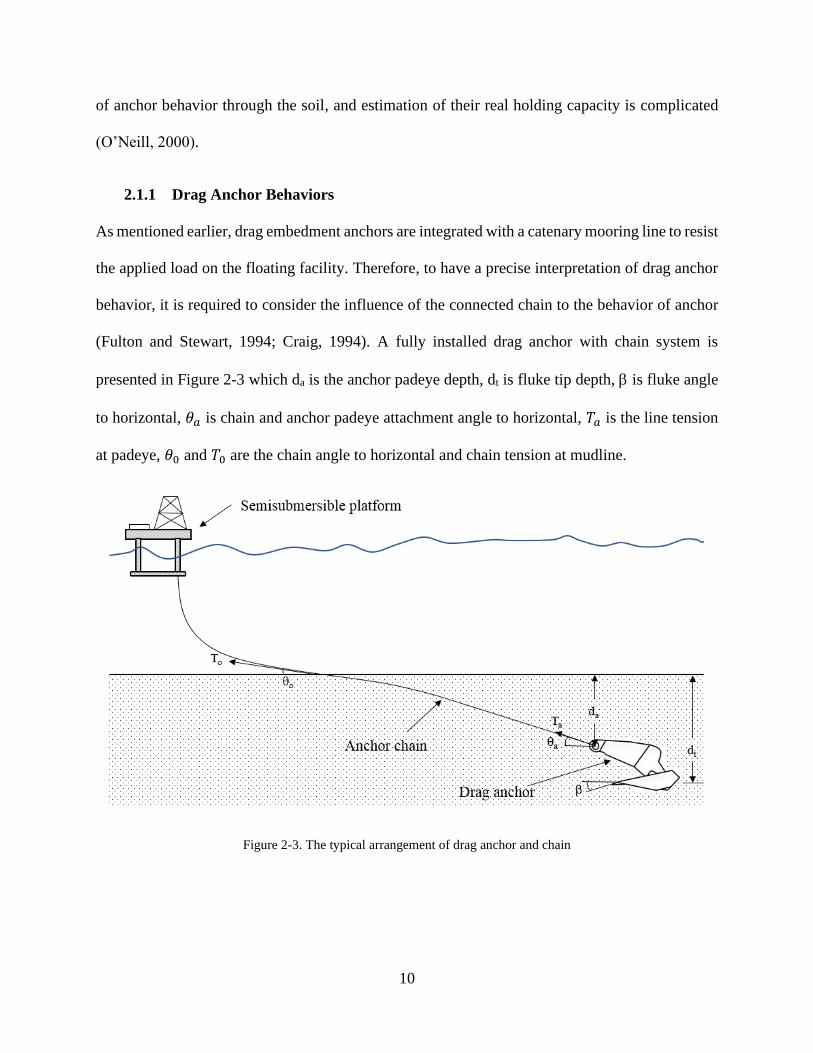
(Fulton and Stewart, 1994; Craig, 1994). A fully installed drag anchor with chain system is
presented in Figure 2-3 which da is the anchor padeye depth, dt is fluke tip depth, is fluke angle
to horizontal, 𝜃𝑎 is chain and anchor padeye attachment angle to horizontal, 𝑇𝑎 is the line tension
at padeye, 𝜃0 and 𝑇0 are the chain angle to horizontal and chain tension at mudline.
Figure 2-3. The typical arrangement of drag anchor and chain
11
2.1.2 Anchor Chain
Three critical points in the anchor chain behavior that should be considered are presented here:
• The line tension angle (𝜃𝑎) at the padeye, which defines the relative magnitude of
horizontal to vertical components of applied force on the anchor. The line tension angle
(𝜃𝑎) need to be kept as small as possible in designs as the drag anchors are supposed to
have a significant horizontal resistance compared to the vertical one.
• The frictional capacity of the buried chain needs to be thoroughly analyzed as the anchor
capacity produced at anchor padeye is strongly dependent on the frictional capacity of the
buried chain (Degenkamp and Dutta, 1989).
• The diameter of the chain has a direct relationship with the frictional capacity and,
consequently, the holding capacity of anchor.
A lot of researchers have been conducted on developing a method to analyze anchor-chain
behavior. The procedure proposed by Vivatrat et al. (1982) and produced by Degenkamp and Dutta
(1989) has been utilized and employed in a series of drag embedment anchor software such as
Stewart Technology Associate (1995), DNV (2000). Subsequently, the proposed method was
utilized by Neubecker and Randolph (1995, 1996a) as an initial step for a theoretical study related
to anchor-chain behavior in homogenous soil and developed by (O’Neill, 2000) for the layered
seabed.
2.1.3 Theoretical Anchor Models
During the last ninety years, a lot of studies and investigations have been done to understand the
behavior of drag anchors and holding capacity in different seabed criteria. Those studies have been
categorized into three main groups to have a better understanding of what has been done before.
12
The first group is drag anchor behavior through experimental investigations, the second group is
developed drag anchor theories, and the last one is design and modeling tools for drag anchors.
a) Drag Anchor Behavior Through Experimental Investigations
The experimental investigations have been done in the laboratory or field tests. The purpose of
those investigations was to find a relation between the holding capacity of anchors and the
geometrical properties of anchors in different soils by the construction of the empirical database.
For example, the NCEL 1987 is one of the most popular field tests, and its results were largely
used in industry as a standard design. NCEL (1987) has design charts that correlate the holding
capacity against the anchor weight.
By introducing the geotechnical centrifuge tests at the start of the 90s, a new method of
experimental tests, especially for drag embedment anchors was introduced as they need long drag
lengths to reach their maximum holding capacity. The results of these tests were utilized for the
evaluation and development of theoretical methods for understanding drag anchors' behavior in
different seabed criteria. For instance, Neubecker (1995) and O’Neill (2000) conducted a series of
centrifuge drag anchor tests in clay and layered soils, respectively.
b) Development of Drag Anchor Theories
Drag anchor theories related to cohesive, non-cohesive soils are developed differently and have
different applications. In comparison between anchors in cohesive and non-cohesive soils, if all
other factors are kept the same, the drag anchors in cohesive soil achieve higher embedment depth
compared to non-cohesive soils. It indicates that failure mechanisms in cohesive soils (clay) are
fully limited and local to the anchor. Still, non-cohesive soils (sand) have an active soil wedge
failure mechanism that goes to the seabed surface. Therefore, the geotechnical forces applied to
13
the anchor in clay soil are not a function of anchor orientation and only dependent to anchor’s local
bearing and shear resistances, and the local undrained shear strength of clay.
Stewart (1992) proposed a theoretical method for drag anchor behavior in clay, which had two
main phases. The first part is a calculation procedure that estimates the major force components
on the fluke and shank of the anchor to determine the net moment on the anchor based on the
center of each force. The second part is related to determining the kinematic of the anchor-based
on the calculated net moment and the assumption that the anchor always moves parallel to its fluke,
which is supported by Dunnavant and Kwan (1993). Based on this study, other researchers
developed the drag anchor theory to calculate the ultimate holding capacity and trajectory of
anchor in clay soil, e.g., Neubecker and Randolph (1996a), Thorne (1998), and O’Neill et al.
(2003).
The general procedure proposed for modeling the drag anchor behavior in the sand is mostly
similar to the clay method, which comprised of static and kinematic analysis to calculate the
geotechnical forces on the anchor components and incremental displacements to compute the
embedment path of the anchor. On the other hand, in non-cohesive soils, geotechnical forces are
higher, penetration depth is lower and, the failure mechanism is extended to the soil surface.
Because the governing geotechnical theory for the calculation of acting forces in non-cohesive
soils completely differs from the cohesive soils.
Saurwalt (1974) proposed the first model to identify the static forces on the drag anchor in the sand
by idealizing the drag anchor with a buried inclined plate. Tabatabaee (1980) and LeLievre and
Tabatabaee (1981) improved the Saurwalt’s work to come up with a procedure to accurately
estimate the holding capacity of anchor for a given depth and orientation in the sand. The first
complete kinematic model of anchor trajectory in sand using a minimum work approach was
14
developed by Neubecker and Randolph (1996b). Using the static and kinematic of drag anchors in
the sand, Neubecker and Randolph (1996c,1996b) formed the model to describe the behavior of
drag anchors in sand.
Despite drag anchor behavior in homogenous soils, there were no studies related to the behavior
of anchor in layered soils before the O’Neill approach. O’Neill (2000) developed the theory of
anchor behavior in the layered seabed (uncemented sand over cemented sand and clay over sand)
using the procedures in clay only and sand only.
c) Design and Modelling Tools for Drag Anchors
All methods above are utilized to come up with some convenient tools for the prediction of anchor
behavior in different criteria. These methods are categorized into three different groups. The first
one is design charts, which predict the holding capacity versus anchor weight in different soils.
For instance: NCEL, Vryhof Stevpris, IFP charts. The second one is design code rules, which have
some recommendations for designing the drag anchor in different criteria, e.g., American
Petroleum Institute's (API) and Det Norske Veritas (DNV). The last one is software designs which
able to predict the behavior of anchors in different soil media and are available commercially such
as, STA-Anchor, DIGIN, UWA-Anchor.
2.2 Buried Subsea Pipelines
As indicated in Figure 2-4, buried subsea pipelines are subjected to movements of seafloor caused
by gravity forces, hydraulic forces, tectonic activity, mudslides, and slumping (Poulos, 1988,
Audibert et al., 1979). These movements could cause instability in the soil surrounding the
pipeline, which may result in rapid and significant displacement of adjacent soil. The resultant
stresses of soil movement depend on different parameters such as soil type, the geometry of

15
pipeline, the existence of trench around the pipe, trench geometry, and native soil and backfill
properties. The scholars have been working to achieve a better understanding of the soil-pipe
interaction, and these studies divided into two broad groups. The first group includes investigations
that consider the soil around the pipeline as a homogenous field. The second group contains studies
that cover the effect of a trench on the pipe-soil interactions.
Figure 2-4. Buried pipeline subjected to ground movement
2.3 Lateral Pipeline Soil Interaction
There are a large number of physical model tests and numerical studies which focus on the lateral
interaction of buried pipes with the surrounding soil in the sand. The physical studies try to
understand the lateral resistance of pipeline using the centrifuge or other experimental methods
and obtain soil failure mechanism using different techniques such as the particle image velocimetry
(PIV). Some of these studies are mentioned here (Trautmann and O’Rourke, 1985; Daiyan et al.,
2011; Almahakeri et al., 2013; Burnett, 2015). Besides physical models, the numerical studies in
the literature use different constitutive models and finite element software to make a better
16
understanding of this complex problem (Yimsiri et al., 2004; Guo and Stolle, 2005; Yimsiri and
Soga, 2006; Xie et al., 2013; Jung et al., 2013).
Despite studies related to pipe soil interaction in the sand, there are only a few theoretical and
experimental pieces of research to find out the lateral resistance of pipeline in clay. As pipelines
have some mutual behavioral characteristics with plate anchors and pipe, some of the studies
related to pipe-soil interaction in clay are developed based on plate anchor or pile theories. For
instance, these studies are done based on plate anchor theory (Tschebotarioff, 1973; Luscher et al.,
1979; Rowe and Davis, 1982; Das et al., 1985; Das et al., 1987; Merifield et al., 2001) and the
following researches are developed using piles principles (Hansen and Christensen, 1961; Reese
and Welch, 1975; Bhushan et al., 1979; Klar and Randolph, 2008).
A limited number of studies in clay have proposed an independent model to investigate the lateral
interaction between soil and pipe (Audibert and Nyman, 1977; Ng, 1994; Paulin, 1998; Oliveira
et al., 2010).
The effect of a trench on the lateral response of the pipe is not well developed. Paulin (1998), C-
CORE (2003), Phillips et al. (2004), Kianian and Shiri (2019) are only researchers that integrated
the effect of a trench and backfill on the lateral pipe-soil interaction in clay.
2.4 Reliability Assessment
Geotechnical engineering always deals with risk and decision making under uncertainty. Even
before the development of any geotechnical disciplines, the people who were dealing with soils,
rocks, and geological phenomena were aware of this fact. Any geotechnical engineering project
comprised of three phases: the first step is site exploration, the second step is the required soil
testing to define the material properties, and the last one is analyzing the response of soil/rock
mass under the applied load. The uncertainty about loads and uncertainty related to foundation

17
response are two significant uncertainties that could be arisen in our geotechnical projects during
all these three phases.
The risked based design and using reliability methods is a practical approach to deal with those
uncertainties and having a more realistic estimation of the real problem. The risk and reliability
methods are used more broadly in offshore structures compared to onshore ones due to the
following reasons, higher construction costs in offshore, the lower ability for maintenance and
service of the structure, and a higher level of uncertainty in offshore due to existence of dynamic
loads (wave, wind, current).
A short review of the utilized reliability tools used in this study is presented in the following
sections.
2.5 Reliability Analysis Methods
The goal of a probabilistic study is to find out how the uncertainty of input parameters in problems
affects the outputs. The first step of performing probabilistic research is developing a model to
solve the problem and calculating the required outputs. After generating the solving model, a limit
state function will be defined based on the conditions of the problem to separate the failure and
the safe zone. Selecting a favorable reliability tool among the existing ones (Monte Carlo
simulation, first and second-order reliability method) will be the next step to carry out the
probabilistic study. It should be mentioned that in a particular geotechnical problem, there are a
large number of parameters that have uncertainty and could be evaluated in probabilistic studies.
Even though based on the purpose of each study, some of them are selected and their uncertainties
will be quantified to see how they will affect the outputs of the problem. The FORM method,
which considers as one of the most crucial reliability tools will be discussed in the next section.
18
2.5.1 First Order Reliability Method (FORM)
In a reliability study, assume 𝑋 = {𝑋1, 𝑋2, … , 𝑋𝑛} represents a set of uncertain parameters involved
in the problem where 𝑋1, 𝑋2, … , 𝑋𝑛 are the probability density function of each parameter, and
𝑓(𝑋) denotes the joint probability function of 𝑋. The limit state function in which distinct safe and
failure regions are indicated by 𝐺(𝑋) and the failure happens whenever 𝐺(𝑋) is less than or equal
to zero. Based on these definitions, the probability of failure could be defined as equation 2-1:
𝑃𝑓 = 𝑃𝑟𝑜𝑏[𝐺(𝑋) < 0] = ∫ 𝑓(𝑋) dX𝐺(𝑋)≤0
(2-1)
Due to difficulties in the calculation of this integral different approximation approaches have been
developed (Madsen et al., 1986). One of the most consistent computational methods is the first
order reliability method (FORM) (Bjerager, 1991).
As stated in equation 2-2, the limit state function 𝐺(𝑋), could be expressed as a function of 𝑅(𝑋)
and 𝑆(𝑋) which are stands for load and capacity:
𝐺 = 𝑅(𝑋) − 𝑆(𝑋) (2-2)
The probability of failure could be calculated using the approximations of the limit state function
𝐺, which is a function of 𝑅 and 𝑆, 𝐺(𝑅, 𝑆). The procedure of the FORM method consists of three
steps (Bjerager, 1991):
I. Transforming limit state function 𝐺(𝑅, 𝑆) into the standard normal space
II. Approximating the modified function in the standard normal space
III. Computing the corresponding probability of failure to the approximate transformed
function
19
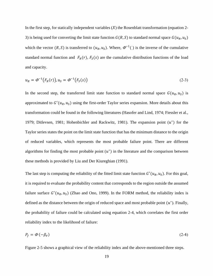
In the first step, for statically independent variables (𝑋) the Rosenblatt transformation (equation 2-
3) is being used for converting the limit state function 𝐺(𝑅, 𝑆) to standard normal space 𝐺(𝑢𝑅 , 𝑢𝑆)
which the vector (𝑅, 𝑆) is transferred to (𝑢𝑅 , 𝑢𝑆). Where, −1( ) is the inverse of the cumulative
standard normal function and 𝐹𝑅(𝑟), 𝐹𝑆(𝑠) are the cumulative distribution functions of the load
and capacity.
𝑢𝑅 = −1(𝐹𝑅(𝑟)), 𝑢𝑆 = −1(𝐹𝑆(𝑠)) (2-3)
In the second step, the transferred limit state function to standard normal space 𝐺(𝑢𝑅 , 𝑢𝑆) is
approximated to 𝐺′(𝑢𝑅 , 𝑢𝑆) using the first-order Taylor series expansion. More details about this
transformation could be found in the following literatures (Hasofer and Lind, 1974; Fiessler et al.,
1979; Ditlevsen, 1981; Hohenbichler and Rackwitz, 1981). The expansion point (𝑢∗) for the
Taylor series states the point on the limit state function that has the minimum distance to the origin
of reduced variables, which represents the most probable failure point. There are different
algorithms for finding the most probable point (𝑢∗) in the literature and the comparison between
these methods is provided by Liu and Der Kiureghian (1991).
The last step is computing the reliability of the fitted limit state function 𝐺′(𝑢𝑅 , 𝑢𝑆). For this goal,
it is required to evaluate the probability content that corresponds to the region outside the assumed
failure surface 𝐺′(𝑢𝑅 , 𝑢𝑆) (Zhao and Ono, 1999). In the FORM method, the reliability index is
defined as the distance between the origin of reduced space and most probable point (𝑢∗). Finally,
the probability of failure could be calculated using equation 2-4, which correlates the first order
reliability index to the likelihood of failure:
𝑃𝑓 = (−𝛽𝐹) (2-4)
Figure 2-5 shows a graphical view of the reliability index and the above-mentioned three steps.
20
Figure 2-5. The graphical interpretation of the reliability index and three steps for the FORM calculation method
2.5.2 Response Surface Method
Sometimes in engineering problems, the function that relates the uncertain input parameters to
outputs of our problem is not easy to develop or implicitly known. For instance, assume the outputs
of a problem are extracted from a large finite element model, which each run takes a long time and
it is not possible to have enough runs for developing the function. Or there is a limited experiment
result that relates the inputs and outputs without any explicit function. If a reliability study needs
to be done in these cases in which there is no explicit function between inputs and outputs, the
response surface method could help to develop a relationship between inputs and outputs based on
the limited available data resources. In the eighties, the response surface method was started to
utilize the reliability assessments of engineering problems (Rackwitz, 1982; Felix and Wong,
1985; Lucia Faravelli, 1990). Subsequently, a large number of studies have been done around the

21
response surface methods and different procedures were developed for applying it to various
engineering problems.
22
Chapter 3. Reliability Assessment of Drag Embedment Anchors in Sand for
Catenary Mooring Systems
Amin Aslkhalili1, Hodjat Shiri1, Sohrab Zendehboudi2
1. Civil Engineering Dept., Faculty of Engineering and Applied Science, Memorial University of
Newfoundland, A1B 3X5, St. John’s, NL, Canada.
2. Process Engineering Dept., Faculty of Engineering and Applied Science, Memorial University
of Newfoundland, A1B 3X5, St. John’s, NL, Canada.
This chapter was published as a journal paper in the “Safety in Extreme Environments-Springer
(2019)” Volume1, Pages39–57, https://doi.org/10.1007/s42797-019-00006-5
23
Abstract
The reliability of drag embedment anchors in sandy seabed was assessed for catenary mooring
systems. The anchor holding capacity was obtained by performing a series of iterative limit state
and kinematic analyses through developing an advanced macro spreadsheet. Series of coupled
dynamic mooring analyses were conducted for a semisubmersible platform using OrcaFlex
software. The dynamic mooring line tensions were obtained by incorporation of the uncertainties
in environmental loads, metocean variables, and stress distribution along the catenary mooring
lines into the response surface. A probabilistic model was developed for holding capacity of the
selected drag anchors. An iterative procedure was performed by adopting the first order reliability
method (FORM) to calculate the failure probabilities. The study showed significant dependence
of the anchoring system reliability on geometrical configuration of the selected anchor families,
the seabed soil properties, and the environmental loads. It was observed that the reliability-based
development of in-filed testing procedures proposed by design codes can have significant
contribution to achieving a more cost-effective and safer design.
Keywords: Reliability analysis; Drag embedment anchor; Catenary mooring; Response surface;
Numerical method; Sand seabed

24
3.1 Introduction
Drag embedment anchors are widely used as a cost-effective solution for temporary and permeant
station keeping of floating structures. By growing offshore exploration and productions, the
number of incidents in floating facilities induced by the failure of mooring system has been
increased, subsequently (Wang et al., 2010; Duggal et al., 2013). This has caused the industry to
further emphasize on reliability assessment of the mooring systems and their key components in
various types of seabed sediments. Drag embedment anchors are amongst the crucial components
of the mooring systems that are used with catenary and taut leg mooring systems.
Different anchoring solutions might be used to provide an efficient and reliable mooring system
such as suction anchors, propellant embedded anchors, screw-in anchors, plate anchors,
deadweight anchors, pile anchors, and drag embedment anchors. However, the latter one is one of
the most attractive options that are simple and cheap to install but challenging to evaluate the
holding capacity (Neubecker and Randolph, 1996a; Aubeny and Chi, 2010) due to complex and
uncertain interaction with the seabed (see Figure 3-1).
Figure 3-1. Detail of drag embedment anchor in the catenary mooring system

25
The current practice proposed by design codes (e.g., API RP 2SK, 2008) recommends a unique
procedure for in-field evaluation of the holding capacity of drag embedment anchors in both sand
and clay. This approach may lead to a different level of reliabilities and cost impacts, consequently.
Therefore, to improve the current practice, it is mandatory to perform comparative reliability
studies for the performance of drag anchors in both sand and clay. There are several studies in the
literature that have considered the reliability assessment of various anchor families such as suction
anchors (Choi, 2007; Valle-molina et al., 2008; Clukey et al., 2013; Silva-González et al., 2013;
Montes-Iturrizaga and Heredia-Zavoni, 2016; Rendón-Conde and Heredia-Zavoni, 2016).
However, having limited access to in-field holding capacity databases, the complicated interaction
between the anchor and the seabed, and the need for the extensive amount of costly computational
analyses have resulted in limitations to assess the reliability of these important Anchor families.
There is only one study that has investigated the reliability of drag anchor in clay (Moharrami and
Shiri, 2018), but there is no study in the sand yet.
The current study contributed to filling of this knowledge gap by combining advanced coupled
mooring analysis and iterative limit state solutions for anchor kinematics in sand seabed that is
quite common in the offshore region. Comparisons were made between the reliability index
provided by the same group of anchors in sand and clay. In addition, an equalization study was
conducted to determine the different group of anchor families in sand and clay that result in an
identical reliability index. The holding capacity of anchors was calculated by developing an Excel
spreadsheet and incorporation of the limit state analysis proposed by Neubecker and Randolph
(1996a). There are several studies on the prediction of drag anchors capacity by analytical and
empirical solutions (Neubecker and Randolph, 1996a; Thorne, 2002; O’Neill et al., 2003; Aubeny
and Chi, 2010). However, the adopted solution (Neubecker and Randolph, 1996a) benefits from

26
several advantages such as simplified prediction of the anchor capacity and trajectory,
incorporation of chain-sand interaction, and comprehensive validation against the experimental
studies ( Neubecker and Randolph, 1996a; Neubecker and Randolph, 1996b; O’Neill et al., 1997).
This model has been widely used in several studies in the literature (Neubecker and Randolph,
1996b; Neubecker and Randolph, 1996c; O’Neill et al., 2003) and recommended by design codes
(e.g., API RP 2SK, 2008).
The mooring line tension was obtained by performing dynamic mooring analysis using OrcaFelx
software and a generic semisubmersible platform. Reliability assessment was performed by using
first-order reliability method (FORM) through developing a probability model for anchor holding
capacities that is further explained in the coming sections.
The study provided an excellent insight into the problem and prepared the ground for improving
the current state-of-practice from reliability and cost-effectiveness standpoints.
3.2 Methodology
The reliability analysis was conducted by calculation of the anchor capacity against the mooring
line tensions. The model proposed by Neubecker and Randolph (1996a) was used to analyze chain-
soil and anchor-soil interactions in the sand and predict the anchor capacity at the mudline and
shank pad-eye. The anchor model was programmed in an Excel spreadsheet VBA Macro (Visual
Basic Application). OrcaFlex software package was employed to model a generic semisubmersible
platform in the Caspian Sea to obtain the characteristic mean and maximum dynamic line tensions
for a 100 years return period sea states. Various key parameters were incorporated in the estimation
of anchor capacities including peak friction at the seabed, dilation angle, soil density, fluke and
shank bearing capacity factors, anchor geometrical configurations, line tension angle at mudline,
and side friction factor. The response surfaces were used to determine the mean and expected
27
maximum dynamic line tensions. First order reliability method (FORM) was used to assess the
reliability of anchors connected to the catenary mooring line. The DNV design code (DNV-RP-
E301, 2012) was used to define the partial design factors on the mean and maximum dynamic line
tensions and capacities.
3.3 Modeling Drag Embedment Anchor
Drag embedment anchors are commonly connected to the chain and then the mooring line. The
resistance that soil provides against the anchor and the frictional capacity of the chain is the
primary source of ultimate anchor capacity. Both of these key components were modeled in the
current study to achieve a sufficient level of accuracy in the calculation of total holding capacity.
3.4 Soil-Chain Interaction
Analysis of the embedded anchor chain is vital for two main reasons. First, the frictional capacity
between the chain and the soil that can significantly contribute to the ultimate anchor capacity.
Second, the angle between the anchor and the chain at the pad eye that has an important effect on
the soil-chain interaction. In the present study, a stud chain was considered, and the methodology
proposed by Neubecker and Randolph (1995) was adopted to implement the chain-soil interaction.
Figure 3-2 shows the free body diagram of a differential segment of the chain that was adopted
force equilibrium analysis (Neubecker and Randolph, 1995a). The parameter T is the line tension;
θ is the inclination from the horizontal; F is the friction force, and Q is the typical soil reaction on
chain segment.

28
Figure 3-2. Force equilibrium of chain element
According to Figure 3-2, the tangential and normal equilibriums can be written as:
𝑑𝑇
𝑑𝑆= 𝐹 + 𝑊𝑆𝑖𝑛𝜃 (3-1)
𝑇𝑑𝜃
𝑑𝑆= −𝑄 + 𝑊𝐶𝑜𝑠𝜃 (3-2)
It is possible to describe the normal (Q) and tangential (F) soil resistances acting on the chain as
soil pressures:
𝑄 = (𝐸𝑛𝑑)𝑞 (3-3)
𝐹 = (𝐸𝑡𝑑)𝑓 (3-4)
where d is the nominal chain diameter, En and Et are circumference parameters. In non-cohesive
soils, the bearing pressure q can be expressed by:
𝑞 = 𝑁𝑞𝛾′𝑧 (3-5)
where q is bearing pressure;Nq is the standard bearing capacity factor; γ′ is the effective unit
weight of the soil; z is depth. These governing equilibrium equations are non-linear which makes
29
difficulties in finding the solution. Therefore, to simplify the equation, the chain was assumed to
be weightless (Neubecker and Randolph, 1995a). Although, it is possible to account for the chain
weight by a secondary effect i.e., reducing the profile of normal resistance per unit length by an
amount equal to the chain weight per unit length. However, Neubecker and Randolph (1995)
showed that the contribution of the chain weight has a minor effect on ultimate capacity. The
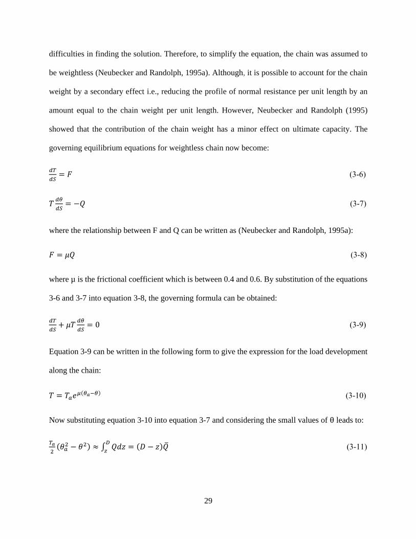
governing equilibrium equations for weightless chain now become:
𝑑𝑇
𝑑𝑆= 𝐹 (3-6)
𝑇𝑑𝜃
𝑑𝑆= −𝑄 (3-7)
where the relationship between F and Q can be written as (Neubecker and Randolph, 1995a):
𝐹 = 𝜇𝑄 (3-8)
where µ is the frictional coefficient which is between 0.4 and 0.6. By substitution of the equations
3-6 and 3-7 into equation 3-8, the governing formula can be obtained:
𝑑𝑇
𝑑𝑆+ 𝜇𝑇
𝑑𝜃
𝑑𝑆= 0 (3-9)
Equation 3-9 can be written in the following form to give the expression for the load development
along the chain:
𝑇 = 𝑇𝑎𝑒𝜇(𝜃𝑎−𝜃) (3-10)
Now substituting equation 3-10 into equation 3-7 and considering the small values of θ leads to:
𝑇𝑎
2(𝜃𝑎
2 − 𝜃2) ≈ ∫ 𝑄𝑑𝑧𝐷
𝑧= (𝐷 − 𝑧)�̅� (3-11)
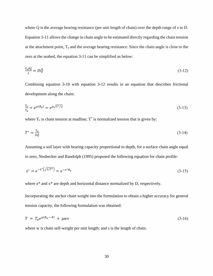
30
where Q is the average bearing resistance (per unit length of chain) over the depth range of z to D.
Equation 3-11 allows the change in chain angle to be estimated directly regarding the chain tension
at the attachment point, Ta and the average bearing resistance. Since the chain angle is close to the
zero at the seabed, the equation 3-11 can be simplified as below:
𝑇𝑎𝜃𝑎2
2= 𝐷�̅� (3-12)
Combining equation 3-10 with equation 3-12 results in an equation that describes frictional
development along the chain:
𝑇𝑜
𝑇𝑎= 𝑒𝜇(𝜃𝑎) = 𝑒𝜇√𝑇∗ 2⁄ (3-13)
where To is chain tension at mudline; T* is normalized tension that is given by:
𝑇∗ =𝑇𝑎
𝐷�̅� (3-14)
Assuming a soil layer with bearing capacity proportional to depth, for a surface chain angle equal
to zero, Neubecker and Randolph (1995) proposed the following equation for chain profile:
𝑧∗ = 𝑒−𝑥∗(√2 𝑇∗⁄ ) = 𝑒−𝑥∗𝜃𝑎 (3-15)
where z* and x* are depth and horizontal distance normalized by D, respectively.
Incorporating the anchor chain weight into the formulation to obtain a higher accuracy for general
tension capacity, the following formulation was obtained:
𝑇 = 𝑇𝑎𝑒𝜇(𝜃𝑎 − 𝜃) + 𝜇𝑤𝑠 (3-16)
where w is chain self-weight per unit length; and s is the length of chain.

31
Figure 3-3 illustrates the validation of the closed form chain profile given in equation 3-16 with
the existing experimental results (Bissett, 1993). The proposed equation is in a good agreement
with a real chain profile, where the bearing resistance is approximately proportional to depth.
Figure 3-3. Comparison of chain profile in sand
3.5 Anchor Holding Capacity
In the present study, the drag anchor was assumed to move through the soil in a quasi-static
condition. Although the anchor has some finite velocity, the magnitude of this velocity is small so
that the inertial considerations can be neglected. To obtain the anchor holding capacity, the limit
state model proposed by Neubecker and Randolph (1996a) was adopted. Figure 3-4 shows the
three-dimensional wedge failure mechanism for calculation of the anchor capacity at pad eye (Ta).

32
Figure 3-4. The three-dimensional failure wedge in plan and side view and force system of the anchor
Using the force equilibrium system shown in Figure 3-4, the first step is to calculate the cross-
section area of the wedge:
𝐴 =𝐻2−ℎ2
2𝑡𝑎𝑛𝛽+
𝐻2𝑡𝑎𝑛𝜆
2 (3-17)
where H is the depth of fluke tips; h is the back edge of the fluke; β is the inclination of the fluke,
and λ is the failure wedge angle. The lateral extent of failure wedge can be calculated by:
𝑋 =𝐻𝑡𝑎𝑛𝜓
𝑐𝑜𝑠 (𝜆−𝜓) (3-18)
where ψ is the dilation angle. Now, the mobilized soil mass can be obtained based on the known
values of X and A:
𝑊𝑠 = 𝛾𝐵𝐴 +2
3𝛾𝑋𝐴 (3-19)
where Ws is the mobilized soil mass; B is the width of the fluke. The side friction (SF) should be
determined to satisfy limit equilibrium formulation:
𝑆𝐹 =𝛾𝐿(𝐻+ℎ)2(𝑠𝑖𝑛∅′−𝑠𝑖𝑛 𝜓)
4𝑐𝑜𝑠𝜓(1−𝑠𝑖𝑛∅′𝑠𝑖𝑛𝜓) (3-20)
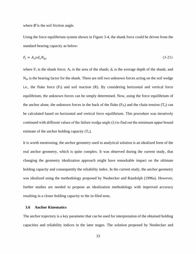
33
where ∅′is the soil friction angle.
Using the force equilibrium system shown in Figure 3-4, the shank force could be driven from the
standard bearing capacity as below:
𝐹𝑠 = 𝐴𝑠𝛾𝑑𝑠𝑁𝑞𝑠 (3-21)
where Fs is the shank force; As is the area of the shank; ds is the average depth of the shank; and
Nqs is the bearing factor for the shank. There are still two unknown forces acting on the soil wedge
i.e., the fluke force (Ff) and soil reaction (R). By considering horizontal and vertical force
equilibrium, the unknown forces can be simply determined. Now, using the force equilibrium of
the anchor alone, the unknown forces in the back of the fluke (Ffb) and the chain tension (Ta) can
be calculated based on horizontal and vertical force equilibrium. This procedure was iteratively
continued with different values of the failure wedge angle (λ) to find out the minimum upper bound
estimate of the anchor holding capacity (Ta).
It is worth mentioning, the anchor geometry used in analytical solution is an idealized form of the
real anchor geometry, which is quite complex. It was observed during the current study, that
changing the geometry idealization approach might have remarkable impact on the ultimate
holding capacity and consequently the reliability index. In the current study, the anchor geometry
was idealized using the methodology proposed by Neubecker and Randolph (1996a). However,
further studies are needed to propose an idealization methodology with improved accuracy
resulting in a closer holding capacity to the in-filed tests.
3.6 Anchor Kinematics
The anchor trajectory is a key parameter that can be used for interpretation of the obtained holding
capacities and reliability indices in the later stages. The solution proposed by Neubecker and

34
Randolph (1996c) for prediction of the anchor trajectory was adopted, where three main conditions
were set to ensure kinematic admissibility of the anchor model. These conditions put constraints
on the absolute and relative displacements of the anchor and the soil wedge and hence are helpful
in defining the kinematics of the system. First, the soil wedge will move at the dilation angle to
the failure surface. Second, displacement of the soil relative to the anchor (dusa) must be parallel
to the upper face of the flukes. Third, the anchor must maintain contact with the soil behind it by
traveling in a direction parallel to the back of the fluke. The third condition applies when there is
a force on the rear of the flukes so that when this force becomes zero, the anchor is free to travel
away from the soil behind it and this condition is meaningless. These three conditions for anchor
and soil displacements fully describe the kinematics of the system so that for a given anchor
displacement the magnitudes and directions of the soil displacement and the relative anchor-soil
displacement can be easily calculated. The minimum work approach was applied and the
penetration ∆𝑦 and rotation ∆𝜃 were considered to obtain the incremental anchor displacements.
Further details of the anchor kinematic model can be found in Neubecker and Randolph (1996c).
3.7 Developing Iterative Macro for Prediction of Anchor Performance
The static limit state and kinematic models were coded into an Excel spreadsheet using VBA
macros to calculate the ultimate holding capacity of the anchor-chain system and the anchor
trajectory. The developed spreadsheet performed a series of iterative analyses with the calculation
procedure outlined in Figure 3-5.
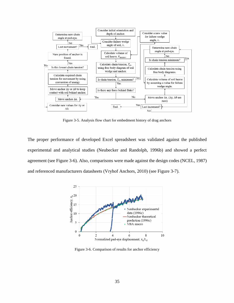
35
Figure 3-5. Analysis flow chart for embedment history of drag anchors
The proper performance of developed Excel spreadsheet was validated against the published
experimental and analytical studies (Neubecker and Randolph, 1996b) and showed a perfect
agreement (see Figure 3-6). Also, comparisons were made against the design codes (NCEL, 1987)
and referenced manufacturers datasheets (Vryhof Anchors, 2010) (see Figure 3-7).
Figure 3-6. Comparison of results for anchor efficiency

36
Figure 3-7. Comparison of results for anchor holding capacity
The input parameters of the validation case study are given in Table 3-1.
Table 3-1. Soil and anchor input parameters in the current analysis
Parameter Value
Anchor dry weight, Wa (kN) 98.06
Fluke length, Lf (m) 3.41
Fluke width, bf (m) 5.99
Fluke thickness, df (m) 0.51
Shank length, Ls (m) 5.55
Shank width, bs (m) 2.31
Fluke-Shank angle, fs () 32
Effective chain width, bc (m) 0.24
Chain self-weight, wc (kN/m) 2
Chain soil friction coefficient, 0.4
Peak friction angle, p () 35
Residual friction angle, r () 25
Dilation angle, () 8.5
Effective unit weight, (kN/m3) 10
3.8 Anchors Used in the Current Study
Two types of popular anchors that are widely used for temporary and permanent mooring of
floating systems, i.e., Stevpris Mk5 and Mk6, were used in the current study for reliability studies.
These anchors have a fluke length to fluke thickness ratios (Lf/df) of 6.67 and 3.09 respectively.

37
Figure 3-8 illustrates the plan and side views of these anchors with geometrical properties given
in Table 3-2. In addition, the selection of these anchors enabled making comparisons with earlier
studies that have used similar anchors (Moharrami and Shiri, 2018).
Figure 3-8. Schematic of the modeled anchor in the present study
Table 3-2. Main dimensions for 12 t anchors (Vryhof Anchors, 2010)
Mk5 (Lf/df = 6.67) Mk6 (Lf/df = 3.09)
A (mm) 5908 5593
B (mm) 6368 6171
C (Lf), (mm) 3624 3961
E (mm) 3010 2642
F (df), (mm) 543 1282
H (mm) 2460 2394
S (mm) 150 140
Fluke-shank angle(θfs), () 32.00 32
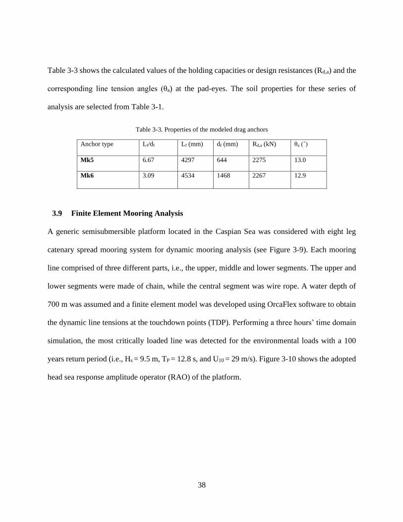
38
Table 3-3 shows the calculated values of the holding capacities or design resistances (Rd,a) and the
corresponding line tension angles (θa) at the pad-eyes. The soil properties for these series of
analysis are selected from Table 3-1.
Table 3-3. Properties of the modeled drag anchors
Anchor type Lf/df Lf (mm) df (mm) Rd,a (kN) θa (˚)
Mk5 6.67 4297 644 2275 13.0
Mk6 3.09 4534 1468 2267 12.9
3.9 Finite Element Mooring Analysis
A generic semisubmersible platform located in the Caspian Sea was considered with eight leg
catenary spread mooring system for dynamic mooring analysis (see Figure 3-9). Each mooring
line comprised of three different parts, i.e., the upper, middle and lower segments. The upper and
lower segments were made of chain, while the central segment was wire rope. A water depth of
700 m was assumed and a finite element model was developed using OrcaFlex software to obtain
the dynamic line tensions at the touchdown points (TDP). Performing a three hours’ time domain
simulation, the most critically loaded line was detected for the environmental loads with a 100
years return period (i.e., Hs = 9.5 m, TP = 12.8 s, and U10 = 29 m/s). Figure 3-10 shows the adopted
head sea response amplitude operator (RAO) of the platform.
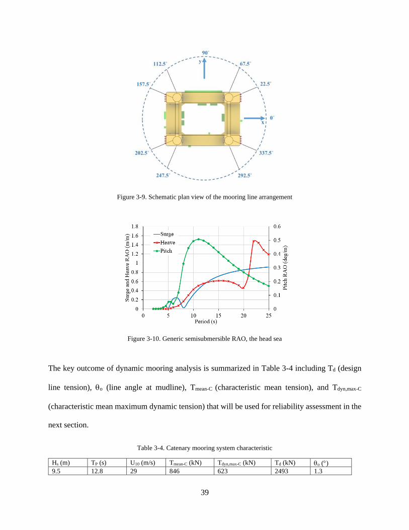
39
Figure 3-9. Schematic plan view of the mooring line arrangement
Figure 3-10. Generic semisubmersible RAO, the head sea
The key outcome of dynamic mooring analysis is summarized in Table 3-4 including Td (design
line tension), o (line angle at mudline), Tmean-C (characteristic mean tension), and Tdyn,max-C
(characteristic mean maximum dynamic tension) that will be used for reliability assessment in the
next section.
Table 3-4. Catenary mooring system characteristic
Hs (m) TP (s) U10 (m/s) Tmean-C (kN) Tdyn,max-C (kN) Td (kN) o ()
9.5 12.8 29 846 623 2493 1.3
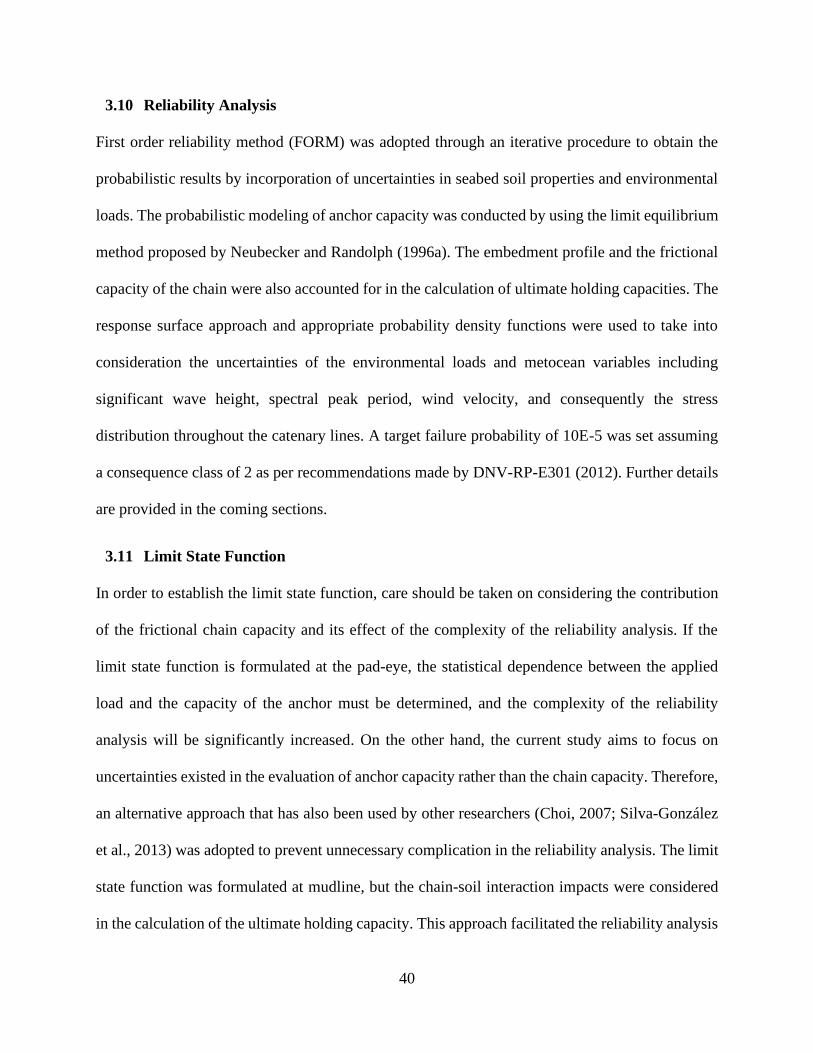
40
3.10 Reliability Analysis
First order reliability method (FORM) was adopted through an iterative procedure to obtain the
probabilistic results by incorporation of uncertainties in seabed soil properties and environmental
loads. The probabilistic modeling of anchor capacity was conducted by using the limit equilibrium
method proposed by Neubecker and Randolph (1996a). The embedment profile and the frictional
capacity of the chain were also accounted for in the calculation of ultimate holding capacities. The
response surface approach and appropriate probability density functions were used to take into
consideration the uncertainties of the environmental loads and metocean variables including
significant wave height, spectral peak period, wind velocity, and consequently the stress
distribution throughout the catenary lines. A target failure probability of 10E-5 was set assuming
a consequence class of 2 as per recommendations made by DNV-RP-E301 (2012). Further details
are provided in the coming sections.
3.11 Limit State Function
In order to establish the limit state function, care should be taken on considering the contribution
of the frictional chain capacity and its effect of the complexity of the reliability analysis. If the
limit state function is formulated at the pad-eye, the statistical dependence between the applied
load and the capacity of the anchor must be determined, and the complexity of the reliability
analysis will be significantly increased. On the other hand, the current study aims to focus on
uncertainties existed in the evaluation of anchor capacity rather than the chain capacity. Therefore,
an alternative approach that has also been used by other researchers (Choi, 2007; Silva-González
et al., 2013) was adopted to prevent unnecessary complication in the reliability analysis. The limit
state function was formulated at mudline, but the chain-soil interaction impacts were considered
in the calculation of the ultimate holding capacity. This approach facilitated the reliability analysis
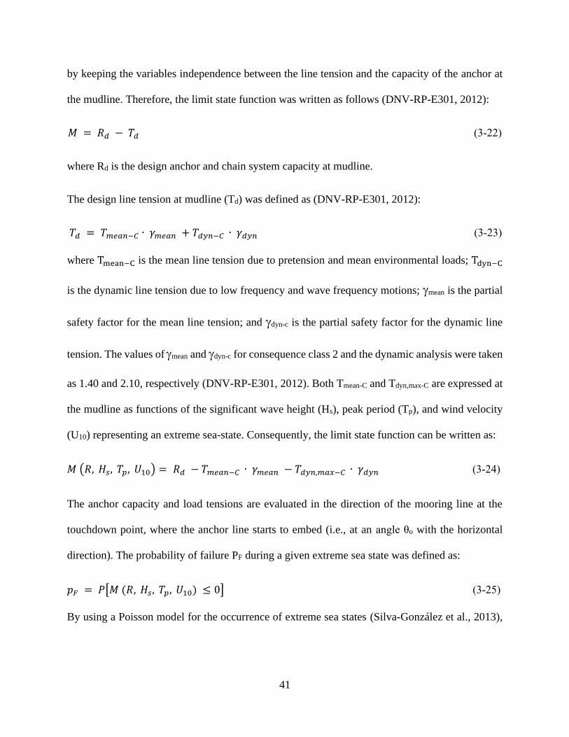
41
by keeping the variables independence between the line tension and the capacity of the anchor at
the mudline. Therefore, the limit state function was written as follows (DNV-RP-E301, 2012):
𝑀 = 𝑅𝑑 − 𝑇𝑑 (3-22)
where Rd is the design anchor and chain system capacity at mudline.
The design line tension at mudline (Td) was defined as (DNV-RP-E301, 2012):
𝑇𝑑 = 𝑇𝑚𝑒𝑎𝑛−𝐶 ∙ 𝛾𝑚𝑒𝑎𝑛 + 𝑇𝑑𝑦𝑛−𝐶 ∙ 𝛾𝑑𝑦𝑛 (3-23)
where Tmean−C is the mean line tension due to pretension and mean environmental loads; Tdyn−C
is the dynamic line tension due to low frequency and wave frequency motions; mean is the partial
safety factor for the mean line tension; and dyn-c is the partial safety factor for the dynamic line
tension. The values of mean and dyn-c for consequence class 2 and the dynamic analysis were taken
as 1.40 and 2.10, respectively (DNV-RP-E301, 2012). Both Tmean-C and Tdyn,max-C are expressed at
the mudline as functions of the significant wave height (Hs), peak period (Tp), and wind velocity
(U10) representing an extreme sea-state. Consequently, the limit state function can be written as:
𝑀 (𝑅, 𝐻𝑠, 𝑇𝑝, 𝑈10) = 𝑅𝑑 − 𝑇𝑚𝑒𝑎𝑛−𝐶 ∙ 𝛾𝑚𝑒𝑎𝑛 − 𝑇𝑑𝑦𝑛,𝑚𝑎𝑥−𝐶 ∙ 𝛾𝑑𝑦𝑛 (3-24)
The anchor capacity and load tensions are evaluated in the direction of the mooring line at the
touchdown point, where the anchor line starts to embed (i.e., at an angle θo with the horizontal
direction). The probability of failure PF during a given extreme sea state was defined as:
𝑝𝐹 = 𝑃[𝑀 (𝑅, 𝐻𝑠, 𝑇𝑝, 𝑈10) ≤ 0] (3-25)
By using a Poisson model for the occurrence of extreme sea states (Silva-González et al., 2013),
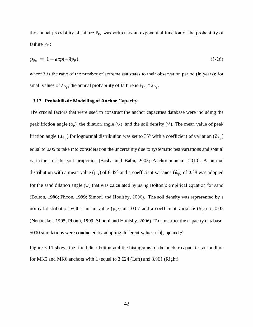
42
the annual probability of failure PFa was written as an exponential function of the probability of
failure PF :
𝑝𝐹𝑎 = 1 − 𝑒𝑥𝑝(−𝜆𝑝𝐹) (3-26)
where λ is the ratio of the number of extreme sea states to their observation period (in years); for
small values of λPF, the annual probability of failure is PFa ≈λPF
.
3.12 Probabilistic Modelling of Anchor Capacity
The crucial factors that were used to construct the anchor capacities database were including the
peak friction angle (p), the dilation angle (), and the soil density (). The mean value of peak
friction angle (μ∅p) for lognormal distribution was set to 35 with a coefficient of variation (δ∅p
)
equal to 0.05 to take into consideration the uncertainty due to systematic test variations and spatial
variations of the soil properties (Basha and Babu, 2008; Anchor manual, 2010). A normal
distribution with a mean value (μ) of 8.49 and a coefficient variance (δ) of 0.28 was adopted
for the sand dilation angle () that was calculated by using Bolton’s empirical equation for sand
(Bolton, 1986; Phoon, 1999; Simoni and Houlsby, 2006). The soil density was represented by a
normal distribution with a mean value (μ𝛾′) of 10.07 and a coefficient variance (δ𝛾′) of 0.02
(Neubecker, 1995; Phoon, 1999; Simoni and Houlsby, 2006). To construct the capacity database,
5000 simulations were conducted by adopting different values of p, and .
Figure 3-11 shows the fitted distribution and the histograms of the anchor capacities at mudline
for MK5 and MK6 anchors with Lf equal to 3.624 (Left) and 3.961 (Right).
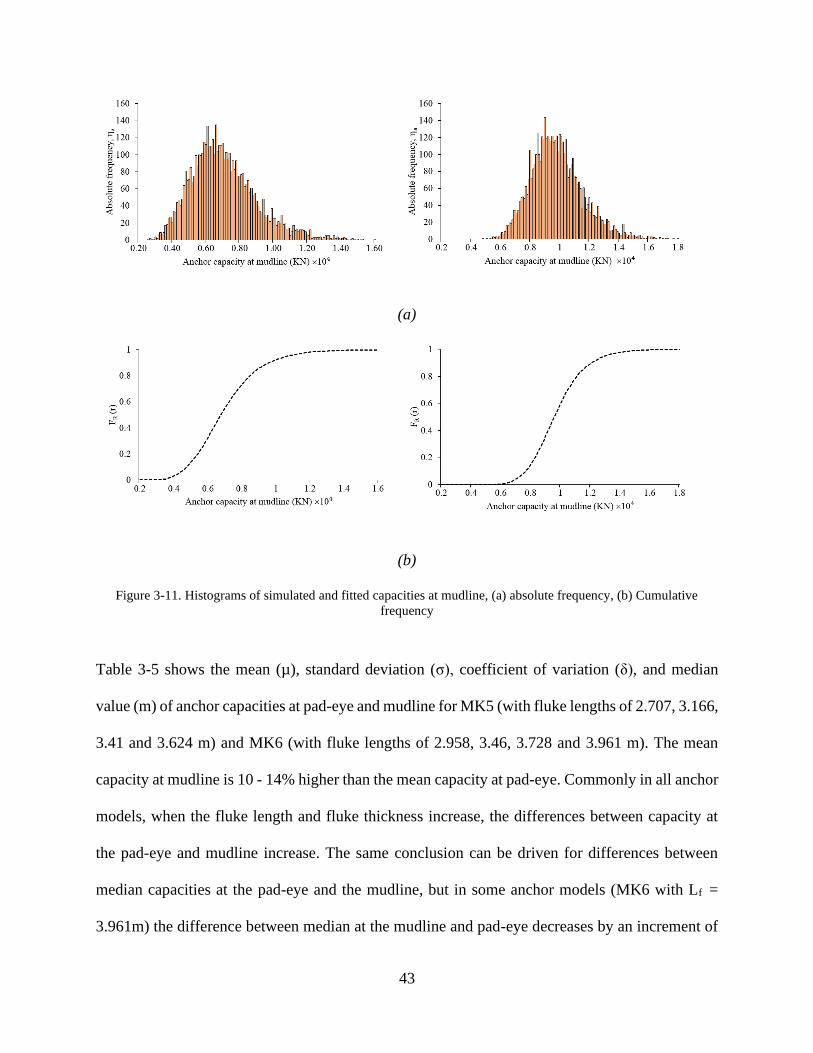
43
(a)
(b)
Figure 3-11. Histograms of simulated and fitted capacities at mudline, (a) absolute frequency, (b) Cumulative
frequency
Table 3-5 shows the mean (µ), standard deviation (σ), coefficient of variation (δ), and median
value (m) of anchor capacities at pad-eye and mudline for MK5 (with fluke lengths of 2.707, 3.166,
3.41 and 3.624 m) and MK6 (with fluke lengths of 2.958, 3.46, 3.728 and 3.961 m). The mean
capacity at mudline is 10 - 14% higher than the mean capacity at pad-eye. Commonly in all anchor
models, when the fluke length and fluke thickness increase, the differences between capacity at
the pad-eye and mudline increase. The same conclusion can be driven for differences between
median capacities at the pad-eye and the mudline, but in some anchor models (MK6 with Lf =
3.961m) the difference between median at the mudline and pad-eye decreases by an increment of
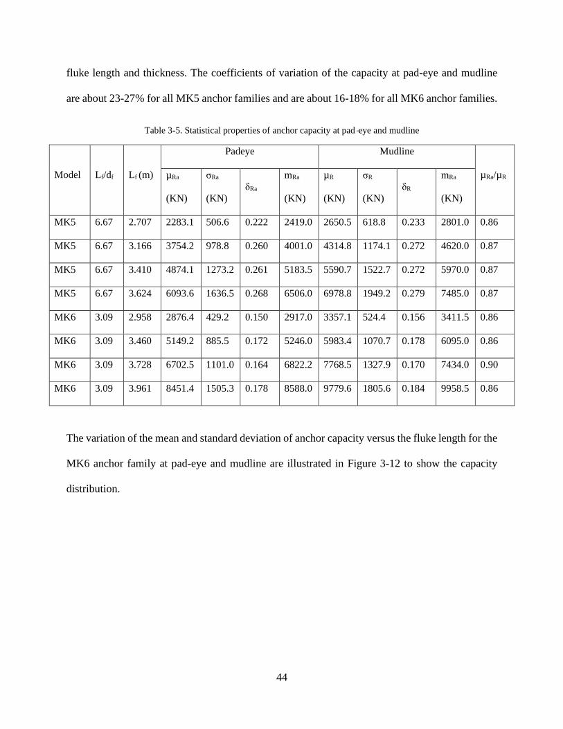
44
fluke length and thickness. The coefficients of variation of the capacity at pad-eye and mudline
are about 23-27% for all MK5 anchor families and are about 16-18% for all MK6 anchor families.
Table 3-5. Statistical properties of anchor capacity at pad-eye and mudline
Model Lf/df Lf (m)
Padeye Mudline
µRa/µR µRa
(KN)
σRa
(KN)
δRa
mRa
(KN)
µR
(KN)
σR
(KN)
δR
mRa
(KN)
MK5 6.67 2.707 2283.1 506.6 0.222 2419.0 2650.5 618.8 0.233 2801.0 0.86
MK5 6.67 3.166 3754.2 978.8 0.260 4001.0 4314.8 1174.1 0.272 4620.0 0.87
MK5 6.67 3.410 4874.1 1273.2 0.261 5183.5 5590.7 1522.7 0.272 5970.0 0.87
MK5 6.67 3.624 6093.6 1636.5 0.268 6506.0 6978.8 1949.2 0.279 7485.0 0.87
MK6 3.09 2.958 2876.4 429.2 0.150 2917.0 3357.1 524.4 0.156 3411.5 0.86
MK6 3.09 3.460 5149.2 885.5 0.172 5246.0 5983.4 1070.7 0.178 6095.0 0.86
MK6 3.09 3.728 6702.5 1101.0 0.164 6822.2 7768.5 1327.9 0.170 7434.0 0.90
MK6 3.09 3.961 8451.4 1505.3 0.178 8588.0 9779.6 1805.6 0.184 9958.5 0.86
The variation of the mean and standard deviation of anchor capacity versus the fluke length for the
MK6 anchor family at pad-eye and mudline are illustrated in Figure 3-12 to show the capacity
distribution.

45
Figure 3-12. The mean and standard deviation of anchor capacity versus fluke length; MK6
3.13 Probabilistic Modelling of Line Tension
The response surfaces were developed using an approach proposed by Silva-González et al.
(2013), where a Gaussian process was adopted to define the dynamic line tensions(Sarkar and
Eatock Taylor, 2000; Choi, 2007). The maximum expected dynamic line tension during the
extreme sea state (presented by a random vector of r uncertain environmental variables (Θ)) was
expressed based on the model proposed by Davenport (1964):
𝐸[𝑇𝑑𝑦𝑛,𝑚𝑎𝑥]𝜃 = 𝜇𝑇𝑑𝑦𝑛,𝑚𝑎𝑥 = [√2𝑙𝑛 (𝜈𝛩𝛥𝑡/2) +0.5772
√2𝑙𝑛 (𝜈𝛩𝛥𝑡/2)] 𝜎𝑇,𝛩 (3-27)
where ∆t is the duration, νΘ = ν(Θ) and σT,Θ = σ(Θ) are the mean crossing rate and the standard
deviation of the dynamic line tension, respectively. A second order polynomial expansion was
used to represent both the line tension Tmean, and the predicted maximum dynamic line tension at
mudline Tdyn, max by using Θ:
𝑌(𝛩) = 𝑐 + 𝑎𝑇𝛩 + 𝛩𝑇𝑏𝛩 (3-28)
Where Y(Θ) is the response of interest, and Θ is the r × 1 vector of environmental variables. The
following unknown coefficients c, a (r ×1) and b (r ×r) were determined by response analysis. To
develop response surfaces, seven key environmental parameters were investigated on the mooring
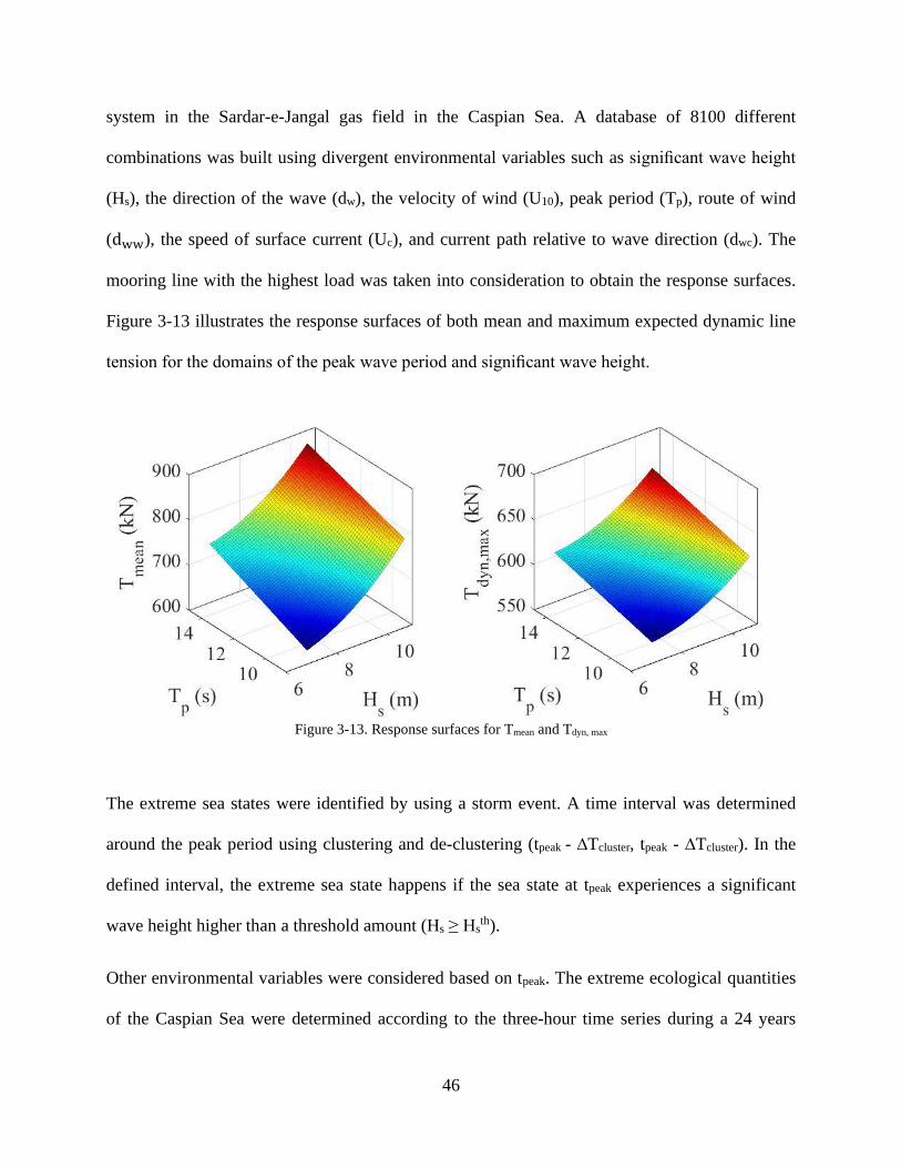
46
system in the Sardar-e-Jangal gas field in the Caspian Sea. A database of 8100 different
combinations was built using divergent environmental variables such as significant wave height
(Hs), the direction of the wave (dw), the velocity of wind (U10), peak period (Tp), route of wind
(dww), the speed of surface current (Uc), and current path relative to wave direction (dwc). The
mooring line with the highest load was taken into consideration to obtain the response surfaces.
Figure 3-13 illustrates the response surfaces of both mean and maximum expected dynamic line
tension for the domains of the peak wave period and significant wave height.
Figure 3-13. Response surfaces for Tmean and Tdyn, max
The extreme sea states were identified by using a storm event. A time interval was determined
around the peak period using clustering and de-clustering (tpeak - ∆Tcluster, tpeak - ∆Tcluster). In the
defined interval, the extreme sea state happens if the sea state at tpeak experiences a significant
wave height higher than a threshold amount (Hs ≥ Hsth).
Other environmental variables were considered based on tpeak. The extreme ecological quantities
of the Caspian Sea were determined according to the three-hour time series during a 24 years
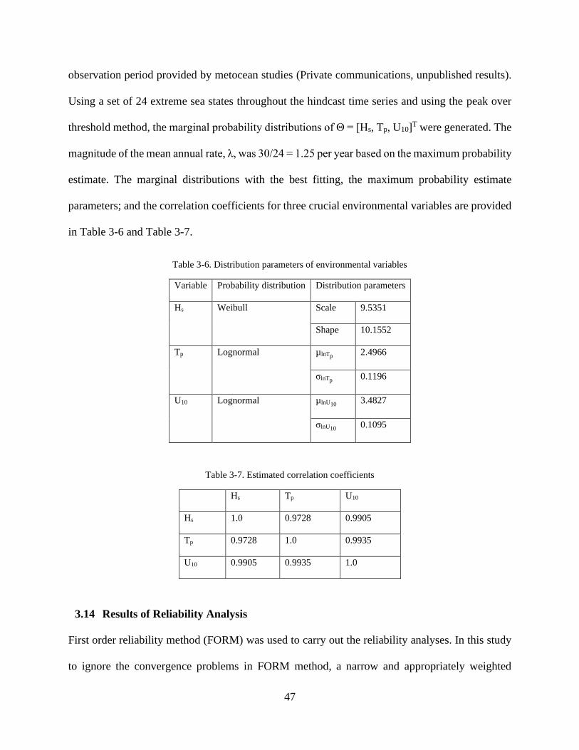
47
observation period provided by metocean studies (Private communications, unpublished results).
Using a set of 24 extreme sea states throughout the hindcast time series and using the peak over
threshold method, the marginal probability distributions of Θ = [Hs, Tp, U10]T were generated. The
magnitude of the mean annual rate, λ, was 30/24 = 1.25 per year based on the maximum probability
estimate. The marginal distributions with the best fitting, the maximum probability estimate
parameters; and the correlation coefficients for three crucial environmental variables are provided
in Table 3-6 and Table 3-7.
Table 3-6. Distribution parameters of environmental variables
Variable Probability distribution Distribution parameters
Hs Weibull Scale 9.5351
Shape 10.1552
Tp Lognormal µlnTp 2.4966
σlnTp 0.1196
U10 Lognormal µlnU10 3.4827
σlnU10 0.1095
Table 3-7. Estimated correlation coefficients
Hs Tp U10
Hs 1.0 0.9728 0.9905
Tp 0.9728 1.0 0.9935
U10 0.9905 0.9935 1.0
3.14 Results of Reliability Analysis
First order reliability method (FORM) was used to carry out the reliability analyses. In this study
to ignore the convergence problems in FORM method, a narrow and appropriately weighted
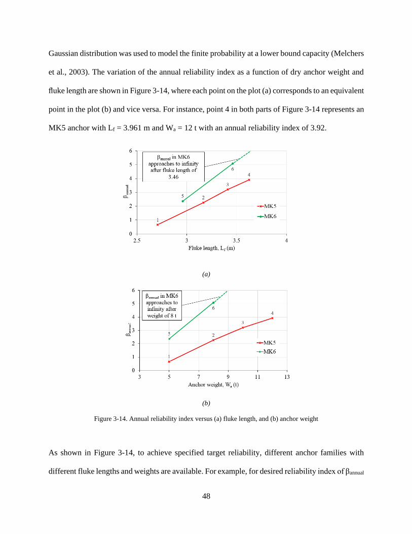
48
Gaussian distribution was used to model the finite probability at a lower bound capacity (Melchers
et al., 2003). The variation of the annual reliability index as a function of dry anchor weight and
fluke length are shown in Figure 3-14, where each point on the plot (a) corresponds to an equivalent
point in the plot (b) and vice versa. For instance, point 4 in both parts of Figure 3-14 represents an
MK5 anchor with Lf = 3.961 m and Wa = 12 t with an annual reliability index of 3.92.
(a)
(b)
Figure 3-14. Annual reliability index versus (a) fluke length, and (b) anchor weight
As shown in Figure 3-14, to achieve specified target reliability, different anchor families with
different fluke lengths and weights are available. For example, for desired reliability index of βannual
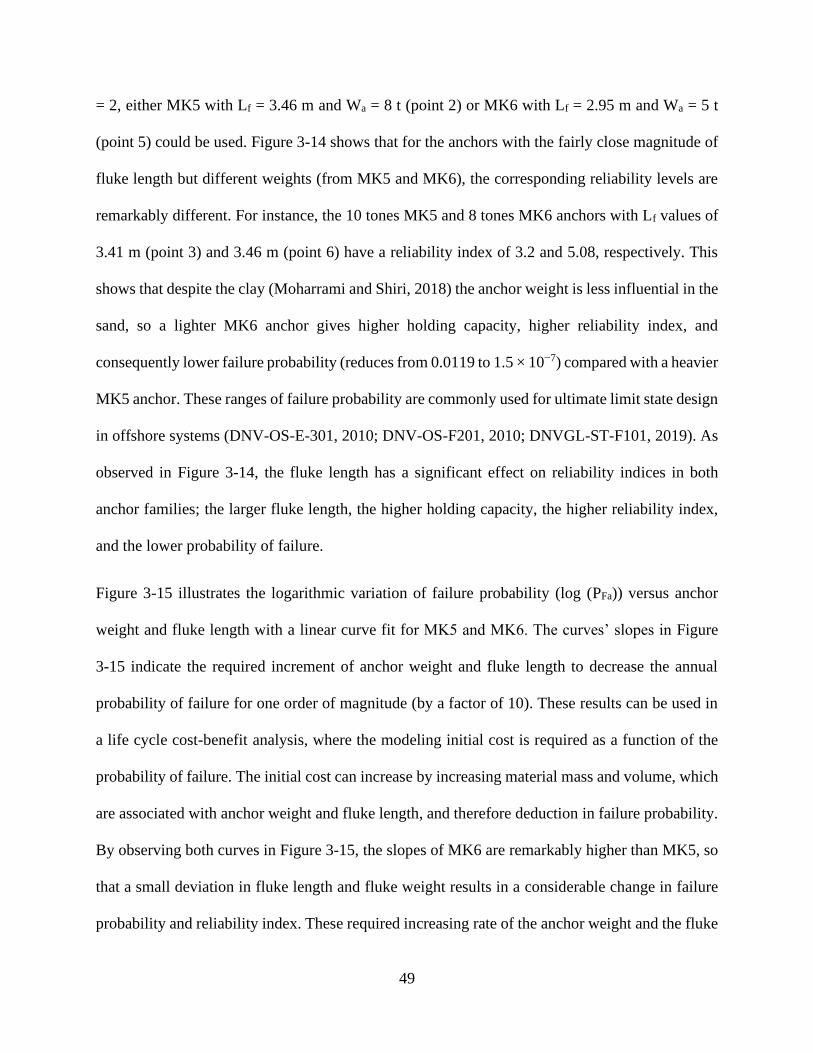
49
= 2, either MK5 with Lf = 3.46 m and Wa = 8 t (point 2) or MK6 with Lf = 2.95 m and Wa = 5 t
(point 5) could be used. Figure 3-14 shows that for the anchors with the fairly close magnitude of
fluke length but different weights (from MK5 and MK6), the corresponding reliability levels are
remarkably different. For instance, the 10 tones MK5 and 8 tones MK6 anchors with Lf values of
3.41 m (point 3) and 3.46 m (point 6) have a reliability index of 3.2 and 5.08, respectively. This
shows that despite the clay (Moharrami and Shiri, 2018) the anchor weight is less influential in the
sand, so a lighter MK6 anchor gives higher holding capacity, higher reliability index, and
consequently lower failure probability (reduces from 0.0119 to 1.5 × 10⁻⁷) compared with a heavier
MK5 anchor. These ranges of failure probability are commonly used for ultimate limit state design
in offshore systems (DNV-OS-E-301, 2010; DNV-OS-F201, 2010; DNVGL-ST-F101, 2019). As
observed in Figure 3-14, the fluke length has a significant effect on reliability indices in both
anchor families; the larger fluke length, the higher holding capacity, the higher reliability index,
and the lower probability of failure.
Figure 3-15 illustrates the logarithmic variation of failure probability (log (PFa)) versus anchor
weight and fluke length with a linear curve fit for MK5 and MK6. The curves’ slopes in Figure
3-15 indicate the required increment of anchor weight and fluke length to decrease the annual
probability of failure for one order of magnitude (by a factor of 10). These results can be used in
a life cycle cost-benefit analysis, where the modeling initial cost is required as a function of the
probability of failure. The initial cost can increase by increasing material mass and volume, which
are associated with anchor weight and fluke length, and therefore deduction in failure probability.
By observing both curves in Figure 3-15, the slopes of MK6 are remarkably higher than MK5, so
that a small deviation in fluke length and fluke weight results in a considerable change in failure
probability and reliability index. These required increasing rate of the anchor weight and the fluke
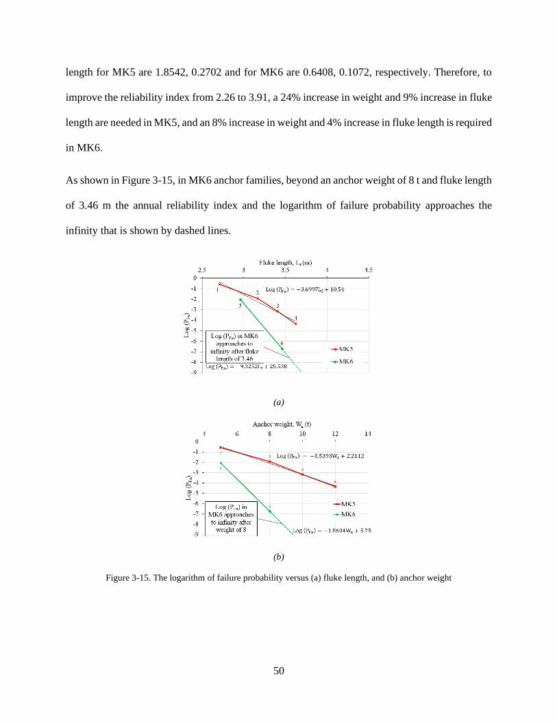
50
length for MK5 are 1.8542, 0.2702 and for MK6 are 0.6408, 0.1072, respectively. Therefore, to
improve the reliability index from 2.26 to 3.91, a 24% increase in weight and 9% increase in fluke
length are needed in MK5, and an 8% increase in weight and 4% increase in fluke length is required
in MK6.
As shown in Figure 3-15, in MK6 anchor families, beyond an anchor weight of 8 t and fluke length
of 3.46 m the annual reliability index and the logarithm of failure probability approaches the
infinity that is shown by dashed lines.
(a)
(b)
Figure 3-15. The logarithm of failure probability versus (a) fluke length, and (b) anchor weight

51
3.15 Equivalent Reliability Study in Sand and Clay
The reliability assessment results obtained from the current study in the sand was compared with
the earlier published studies in clay (Moharrami and Shiri, 2018) to provide an in-depth insight
into the problem. The comparative reliability assessment was conducted to determine the anchor
classes (commonly referred to by their weight in practice) resulting in similar reliability indices.
Figure 3-16 shows the comparative reliability indices obtained for different anchor weights from
MK5 and MK6 families in sand and clay. The plots show the anchor classes in sand and clay that
result in a fairly close magnitude of reliability indices. For instance, an 8 t MK5 anchor in the sand
(point 1) results in an almost same reliability index (2.26 and 2.48) given by a 15 t MK5 anchor in
clay (point 5). In MK6, the reliability indices of anchors heavier than 8 t are infinity, so there are
only two points for sand.
(MK5)
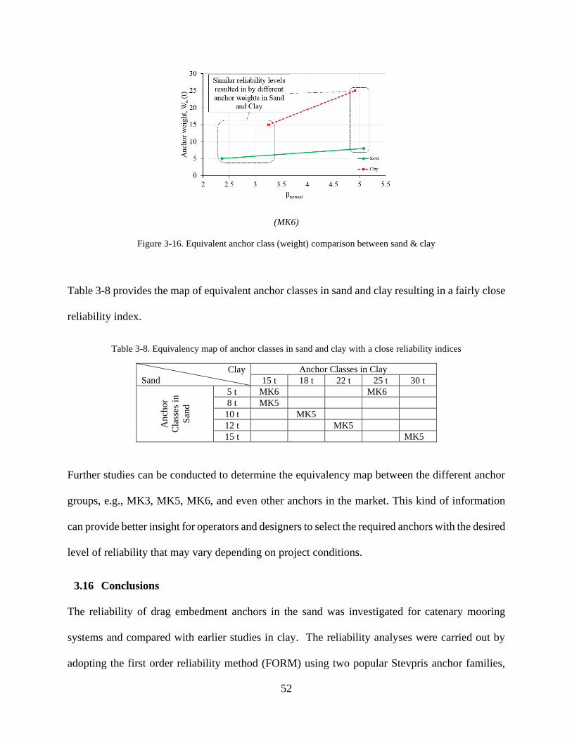
52
(MK6)
Figure 3-16. Equivalent anchor class (weight) comparison between sand & clay
Table 3-8 provides the map of equivalent anchor classes in sand and clay resulting in a fairly close
reliability index.
Table 3-8. Equivalency map of anchor classes in sand and clay with a close reliability indices
Clay
Sand
Anchor Classes in Clay
15 t 18 t 22 t 25 t 30 t
An
cho
r
Cla
sses
in
San
d
5 t MK6 MK6
8 t MK5
10 t MK5
12 t MK5
15 t MK5
Further studies can be conducted to determine the equivalency map between the different anchor
groups, e.g., MK3, MK5, MK6, and even other anchors in the market. This kind of information
can provide better insight for operators and designers to select the required anchors with the desired
level of reliability that may vary depending on project conditions.
3.16 Conclusions
The reliability of drag embedment anchors in the sand was investigated for catenary mooring
systems and compared with earlier studies in clay. The reliability analyses were carried out by
adopting the first order reliability method (FORM) using two popular Stevpris anchor families,

53
MK5 and MK6. The limit state function was established at the mudline, while the chain-soil
interaction effects were accounted for in the calculation of ultimate holding capacities. Fully
coupled time domain analyses were conducted to simulate the station keeping of a generic
semisubmersible platform in the Caspian Sea and obtain the dynamic mooring line tensions.
Response surface method was adopted for probabilistic modeling of the line tensions at mudline.
An Excel spreadsheet containing VBA macros was developed and validated to predict the ultimate
anchor capacity and the anchor trajectory down the seabed by incorporation of a popular limit state
model in the sand. The variation of annual reliability indices and the logarithm of the failure
probabilities versus the fluke length and the anchor weight were obtained and compared with
existing studies. Several important trends were observed, some of which are summarized as
follows:
The geometrical configuration of the anchors, particularly the fluke length, are the most influential
parameters in determining the reliability indices. The anchor weight has a beneficial contribution
to achieving a higher level of reliability but to a less extent. A well-designed anchor geometry can
significantly dominate the weight effect. For instance, some lighter MK6 anchors result in a higher
reliability index compared to heavier MK5 models due to their superior geometrical design.
The costly in-field testing procedure recommended by design codes for estimation of the anchor
capacities are unique for all of the anchor families, seabed soil types, environmental loads, and
operation conditions. This approach ignores the reliability effects affected by a wide range of
inherent uncertainties and limits the cost-effectiveness of the proposed solutions. Further
reliability-based refinement of the proposed procedures can have significant cost effects on
offshore projects.

54
The existing anchor solutions are developed based on simplified anchor geometries. The
idealization of anchor geometry may have a significant impact on reliability results. However, the
impact is not significant in comparative studies. Further investigations are required to determine
the best practice for the idealization of anchor geometry in analytical solutions.
A target reliability index for a given anchor family in clay can be achieved by a heavier anchor
compared to the sand. It is challenging to determine a corresponding set of soil parameters in clay
and sand to result in an identical reliability index. However, further studies in this area can be
beneficial in proposing a more cost-effective infield testing procedure.
It is worth mentioning that the reliability models for assessing the anchor capacities can be
significantly improved by having access to the in-field test databases and corresponding seabed
soil properties, and the statistics of failures. These kinds of information are mandatory for
obtaining absolute reliability indices or failure probabilities. However, the closed form solution is
highly beneficial for performing comparative studies and improving the recommended practices.
Acknowledgments
The authors gratefully acknowledge the financial support of this research by Wood PLC via
establishing the Wood Group Chair in Arctic and harsh environment engineering at Memorial
University, the NL Tourism, Culture, Industry and Innovation (TCII) via CRD collaborative
funding program, the Natural Sciences and Engineering Research Council of Canada (NSERC)
via Engage funding program, Memorial University of Newfoundland through VP start-up fund
and school of graduate studies (SGS). The technical advice of Mr. Mohammad Javad Moharrami
is also kindly acknowledged.
55
References
API RP 2SK, 2008. Design and Analysis of Stationkeeping Systems for Floating Structures.
Aubeny, C.P., Chi, C., 2010. Mechanics of Drag Embedment Anchors in a Soft Seabed. J. Geotech.
Geoenvironmental Eng. 136, 57–68. https://doi.org/10.1061/(ASCE)GT.1943-5606.0000198
Basha, B.M., Babu, G.L.S., 2008. Target reliability based design optimization of anchored
cantilever sheet pile walls. Can. Geotech. J. 45, 535–548. https://doi.org/10.1139/t08-004
Bissett, M.J., 1993. Soil resistance to chain anchor movement.
Bolton, M.D., 1986. Discussion: The strength and dilatancy of sands. Géotechnique 37, 219–226.
https://doi.org/10.1680/geot.1987.37.2.219
Choi, Y.J., 2007. Reliability Assessment of Foundations for Offshore Mooring Systems under
Extreme Environments.
Clukey, E.C., Gilbert, R.B., Andersen, K.H., Dahlberg, R., 2013. Reliability of Suction Caissons
for Deep Water Floating Facilities 1991, 456–474. https://doi.org/10.1061/9780784412763.035
Davenport, A.G., 1964. Note on the Distribution of the Largest Value of a Random Function With
Application To Gust Loading. Proc. Inst. Civ. Eng. 28, 187–196.
https://doi.org/10.1680/iicep.1964.10112
DNV-OS-E-301, 2010. Position Mooring. Offshore Standard.
DNV-OS-F201, 2010. Dynamic Risers. Offshore Standard.
DNV-RP-E301, 2012. Design and Installation of Fluke Anchors.
DNVGL-ST-F101, 2019. Submarine Pipeline Systems. Offshore standartd.

56
Duggal, A., Ma, K., Shu, H., Smedley, P., L'Hostis, D., 2013. A Historical Review on
Integrity Issues of Permanent Mooring Systems 3. https://doi.org/10.4043/24025-ms
Melchers, R.E., Ahammed, M., Middleton, C., 2003. FORM for discontinuous and truncated
probability density functions. Struct. Saf. 25, 305–313. https://doi.org/10.1016/S0167-
4730(03)00002-X
Moharrami, M.J., Shiri, H., 2018. Reliability assessment of drag embedment anchors in clay for
catenary mooring systems. Mar. Struct. 58, 342–360.
https://doi.org/10.1016/j.marstruc.2017.12.005
Montes-Iturrizaga, R., Heredia-Zavoni, E., 2016. Reliability analysis of mooring lines using
copulas to model statistical dependence of environmental variables. Appl. Ocean Res. 59, 564–
576. https://doi.org/10.1016/j.apor.2016.07.008
NCEL, 1987. Drag embedment anchors for navy moorings. Naval Civil Engineering Laboratory,
Port Hueneme, Calif., Techdata Sheet 83-08R.
Neubecker, S.R., 1995. The behaviour of drag anchor and chain systems, PhD Thesis, Department
of Civil Engineering, The University of Western Australia.
Neubecker, S.R., Randolph, M.F., 1996a. The performance of drag anchor and chain systems in
cohesive soil. Georesources Geotech. 14, 1–7.
Neubecker, S.R., Randolph, M.F., 1996b. The kinematic behaviour of drag anchors in sand. Can.
Geotech. J. 33, 584–594. https://doi.org/https://doi.org/10.1139/t96-084-306
Neubecker, S.R., Randolph, M.F., 1996c. The static equilibrium of drag anchors in sand. Can.
Geotech. J. 33, 574–583.

57
Neubecker, S.R., Randolph, M.F., 1995. Profile and frictional capacity of embedded anchor
chains. Geotech. Eng. 121, 797–803.
O’Neill, M.P., Bransby, M.F., Randolph, M.F., 2003. Drag anchor fluke–soil interaction in clays.
Can. Geotech. J. 40, 78–94. https://doi.org/10.1139/t02-096
O’Neill, M.P., Randolph, M.F., Neubecker, S.R., 1997. A Novel Procedure For Testing Model
Drag Anchors, in: Proceedings of the 7th International Offshore and Polar Engineering
Conference.
Phoon, K.K., 1999. Characterization of geotechnical variability. Can. Geotech. J. 624, 612–624.
Private communications, n.d. with Kinsale Energy Ltd.
Rendón-Conde, C., Heredia-Zavoni, E., 2016. Reliability analysis of suction caissons for moored
structures under parameter uncertainties. Struct. Saf. 60, 102–116.
https://doi.org/10.1016/j.strusafe.2016.02.004
Sarkar, A., Eatock Taylor, R., 2000. Effects of mooring line drag damping on response statistics
of vessels excited by first- and second-order wave forces. Ocean Eng. 27, 667–686.
https://doi.org/10.1016/S0029-8018(99)00014-1
Silva-González, F., Heredia-Zavoni, E., Valle-Molina, C., Sánchez-Moreno, J., Gilbert, R.B.,
2013. Reliabilitystudy of suction caissons for catenary and taut-leg mooring systems. Struct. Saf.
45, 59–70. https://doi.org/10.1016/j.strusafe.2013.08.011
Simoni, A., Houlsby, G.T., 2006. The direct shear strength and dilatancy of sand-gravel mixtures.
Geotech. Geol. Eng. 24, 523–549. https://doi.org/10.1007/s10706-004-5832-6
58
Thorne, C.P., 2002. Penetration and Load Capacity of Marine Drag Anchors in Soft Clay. J.
Geotech. Geoenvironmental Eng. 124, 945–953. https://doi.org/10.1061/(asce)1090-
0241(1998)124:10(945)
Valle-molina, C., Heredia-zavoni, E., Silva-gonzález, F.L., 2008. Reliability analyses of suction
caissons for FPSO systems, in: International Conference on Offshore Mechanics and Arctic
Engineering. pp. 1–6.
Vryhof Anchors, 2010. Anchor manual. Krimpen ad Yssel, The Netherlands.
Wang, L.Z., Guo, Z., Yuan, F., 2010. Quasi-static three-dimensional analysis of suction anchor
mooring system. Ocean Eng. 37, 1127–1138. https://doi.org/10.1016/j.oceaneng.2010.05.002
59
Chapter 4. Reliability Assessment of Drag Embedment Anchors in Layered
Seabed, Clay over Sand
Amin Aslkhalili1, Hodjat Shiri2
1. 2. Civil Engineering Dept., Faculty of Engineering and Applied Science, Memorial
University of Newfoundland, A1B 3X5, St. John’s, NL, Canada.
This chapter is a conference paper accepted for oral presentation in 73rd Canadian Geotechnical
Conference (Geo-Calgary2020), Paper number 71.
60
Abstract
Drag embedment anchors combined with catenary mooring systems are widely used for temporary
and permeant station keeping of the offshore floating facilities. With growing exploration and
production of offshore reserves, the number of mooring failure incidents in floating facilities has
been increased. This implies the significance of the reliability assessment of the mooring system
components and particularly drag embedment anchors as one of the key elements. The currently
used anchor design codes consider only homogeneous seabed soil condition. It is widely accepted
that the presence of the layered seabed may significantly affect the ultimate holding capacity of
anchors. Therefore, it is expected that layered seabed condition affects the reliability indices of
these anchors as well. However, there are only a few published studies that have investigated
homogeneous seabed soil condition ignoring the effect of layered soil strata. In this study, the
reliability of drag embedment anchors was comprehensively investigated in the layered seabed
(clay over sand). An advanced calculation tool was developed to obtain the holding capacity of the
anchors by combining a series of iterative limit state and kinematic analysis. A time-domain
dynamic mooring analysis was conducted by assuming a semisubmersible platform to obtain the
dynamic line tensions. The uncertainties of the environmental loads, metocean variables, seabed
soil properties were incorporated into a first-order reliability analysis (FORM) to obtain the failure
probabilities. A probabilistic model established for determination of holding the capacity for
nominated drag anchor families. The study revealed a significant effect of the layered soil
condition in reliability assessment by lowering the magnitude of reliability indices. The
improvement of the recommendations provided by design codes by incorporation of the complex
seabed condition was found necessary for a safer and cost-effective anchor design.
61
Keywords: Drag embedment anchors; Reliability assessment; Surface response; Layered seabed
soil; Probabilistic modeling; Dynamic mooring analysis
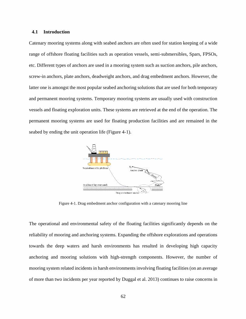
62
4.1 Introduction
Catenary mooring systems along with seabed anchors are often used for station keeping of a wide
range of offshore floating facilities such as operation vessels, semi-submersibles, Spars, FPSOs,
etc. Different types of anchors are used in a mooring system such as suction anchors, pile anchors,
screw-in anchors, plate anchors, deadweight anchors, and drag embedment anchors. However, the
latter one is amongst the most popular seabed anchoring solutions that are used for both temporary
and permanent mooring systems. Temporary mooring systems are usually used with construction
vessels and floating exploration units. These systems are retrieved at the end of the operation. The
permanent mooring systems are used for floating production facilities and are remained in the
seabed by ending the unit operation life (Figure 4-1).
Figure 4-1. Drag embedment anchor configuration with a catenary mooring line
The operational and environmental safety of the floating facilities significantly depends on the
reliability of mooring and anchoring systems. Expanding the offshore explorations and operations
towards the deep waters and harsh environments has resulted in developing high capacity
anchoring and mooring solutions with high-strength components. However, the number of
mooring system related incidents in harsh environments involving floating facilities (on an average
of more than two incidents per year reported by Duggal et al. 2013) continues to raise concerns in

63
the industry in general. On the other hand, large uncertainties in seabed parameters and
environmental loads combined with the inaccessibility for monitoring, inspection, and
maintenance mandates the reliability assessment of drag anchors to minimize their likelihood of
failure.
It becomes more challenging when the seabed soil strata comprise of layered conditions such as
clay over sand, sand over clay, sand over sand, etc., since depending on the anchor trajectory in
the layered soil, the ultimate holding capacity may significantly vary (M. P. O’Neill et al., 1997).
In layered seabed condition, the existing design codes recommend the same capacity assessment
procedure as homogeneous soil. This simplification may affect the reliability of the drag anchors
and impose some level of risk to the project. This important aspect has never been studied in the
past and needs investigations to facilitate refining the design code recommendations for layered
soil.
The holding capacity of drag embedment anchors has been widely investigated (Dunnavant and
Kwan, 1993; Neubecker, 1995; Neubecker and Randolph, 1996; O’Neill et al., 1997; O’Neill,
2000; O’Neill et al., 2003). The reliability of some of the anchor families such as suction caissons
have been widely investigated in the literature (Clukey et al., 2013; Choi, 2007; Valle-molina et
al., 2008; Silva-González et al., 2013; Montes-Iturrizaga and Heredia-Zavoni, 2016; Rendón-
Conde and Heredia-Zavoni, 2016). However, there are only two studies (to the best of the authors’
knowledge) on the reliability of drag embedment anchors (Moharrami and Shiri, 2018; Aslkhalili
et al., 2019) both of which have considered a single homogeneous layer of clay and sand,
respectively.
In this study, the influence of layered seabed on reliability and the likelihood of failure of drag
embedment anchors supporting the catenary mooring lines were comprehensively investigated.
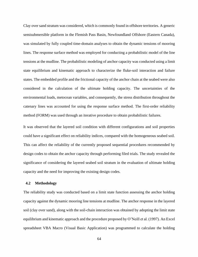
64
Clay over sand stratum was considered, which is commonly found in offshore territories. A generic
semisubmersible platform in the Flemish Pass Basin, Newfoundland Offshore (Eastern Canada),
was simulated by fully coupled time-domain analyses to obtain the dynamic tensions of mooring
lines. The response surface method was employed for conducting a probabilistic model of the line
tensions at the mudline. The probabilistic modeling of anchor capacity was conducted using a limit
state equilibrium and kinematic approach to characterize the fluke-soil interaction and failure
states. The embedded profile and the frictional capacity of the anchor chain at the seabed were also
considered in the calculation of the ultimate holding capacity. The uncertainties of the
environmental loads, metocean variables, and consequently, the stress distribution throughout the
catenary lines was accounted for using the response surface method. The first-order reliability
method (FORM) was used through an iterative procedure to obtain probabilistic failures.
It was observed that the layered soil condition with different configurations and soil properties
could have a significant effect on reliability indices, compared with the homogeneous seabed soil.
This can affect the reliability of the currently proposed sequential procedures recommended by
design codes to obtain the anchor capacity through performing filed trials. The study revealed the
significance of considering the layered seabed soil stratum in the evaluation of ultimate holding
capacity and the need for improving the existing design codes.
4.2 Methodology
The reliability study was conducted based on a limit state function assessing the anchor holding
capacity against the dynamic mooring line tensions at mudline. The anchor response in the layered
soil (clay over sand), along with the soil-chain interaction was obtained by adopting the limit state
equilibrium and kinematic approach and the procedure proposed by O’Neill et al. (1997). An Excel
spreadsheet VBA Macro (Visual Basic Application) was programmed to calculate the holding

65
capacity of anchor incorporating the effect of the soil-chain interaction. In order to obtain the mean
and maximum dynamic line tensions, mooring analysis was conducted using OrcaFelx by
assuming a generic semisubmersible platform in the Flemish Pass Basin, NL offshore (Canada),
and the sea states with a 100 years return period.
Stevpris Mk5 and Mk6 anchors were considered for reliability studies with the key parameters
including undrained shear strength, effective clay unit weight, fluke and shank bearing factor, clay
and sand boundary layer depth, effective sand unit weight, sand friction angle, dilation angle,
anchor geometrical configurations, line tension angle at mudline, and side friction factor. The
response surface method was used to function the mean and predicted maximum of dynamic line
tension using uncertain metocean variables. The reliability analysis was conducted by using the
first order reliability method (FORM). The required data related to partial design factors for
capacities and the mean and maximum dynamic line tensions were obtained from DNV-RP-E301
(2012).
4.3 Modeling Drag Anchor in Layered Soil
4.3.1 Chain-Soil frictional capacity
The frictional capacity between the soil and the embedded chain has a significant contribution to
the anchor performance, penetration trajectory, and the ultimate holding capacity (Neubecker and
Randolph, 1995a). The model proposed by O’Neill et al. (1997) was adopted to calculate the soil-
chain frictional capacity in layered soil. This model has been developed by extension of the earlier
studies conducted by Neubecker and Randolph (1995b). Figure 4-2 shows the force equilibrium
of the chain, where Q is the soil bearing resistance normal to the chain, T is the line tension, F is
the friction force, and is inclination angle from the horizontal line.
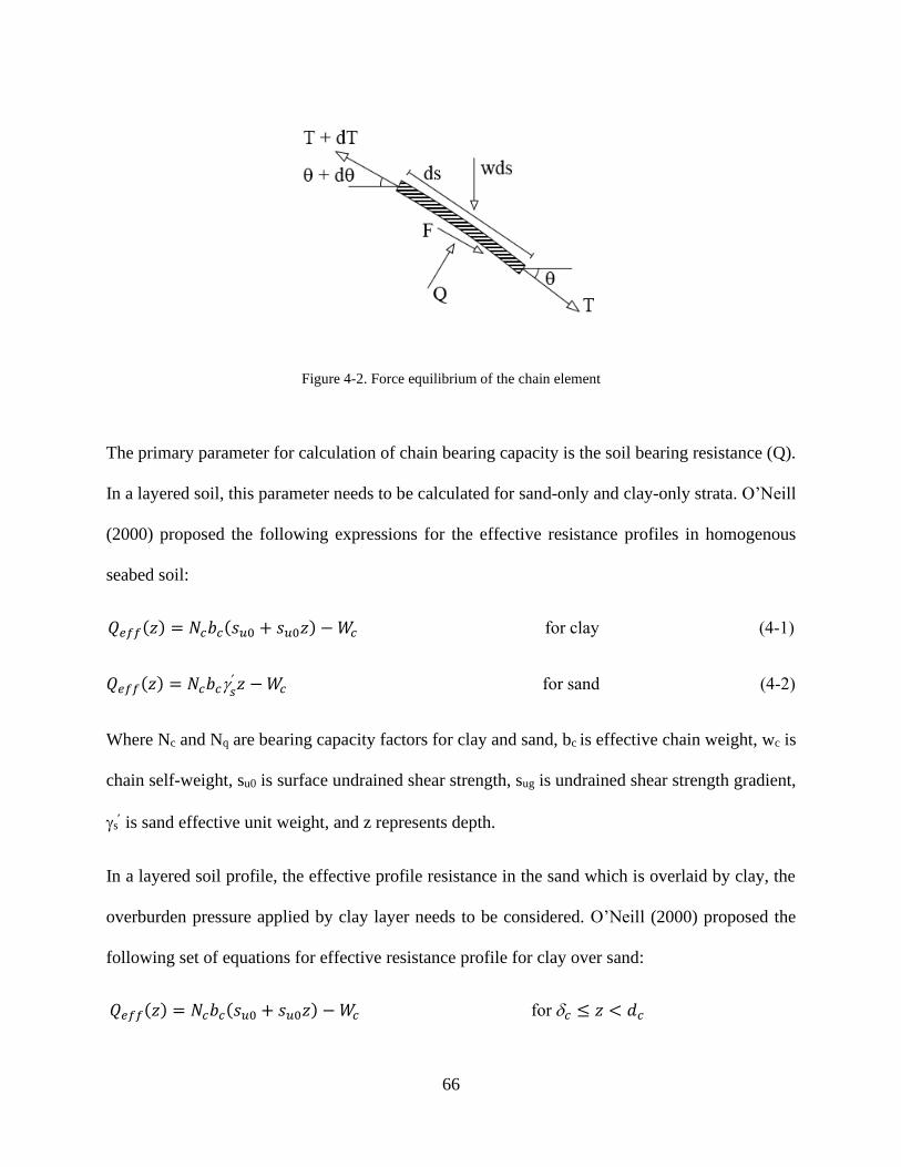
66
Figure 4-2. Force equilibrium of the chain element
The primary parameter for calculation of chain bearing capacity is the soil bearing resistance (Q).
In a layered soil, this parameter needs to be calculated for sand-only and clay-only strata. O’Neill
(2000) proposed the following expressions for the effective resistance profiles in homogenous
seabed soil:
𝑄𝑒𝑓𝑓(𝑧) = 𝑁𝑐𝑏𝑐(𝑠𝑢0 + 𝑠𝑢0𝑧) − 𝑊𝑐 for clay (4-1)
𝑄𝑒𝑓𝑓(𝑧) = 𝑁𝑐𝑏𝑐𝑠 𝑧 − 𝑊𝑐 for sand (4-2)
Where Nc and Nq are bearing capacity factors for clay and sand, bc is effective chain weight, wc is
chain self-weight, su0 is surface undrained shear strength, sug is undrained shear strength gradient,
s is sand effective unit weight, and z represents depth.
In a layered soil profile, the effective profile resistance in the sand which is overlaid by clay, the
overburden pressure applied by clay layer needs to be considered. O’Neill (2000) proposed the
following set of equations for effective resistance profile for clay over sand:
𝑄𝑒𝑓𝑓(𝑧) = 𝑁𝑐𝑏𝑐(𝑠𝑢0 + 𝑠𝑢0𝑧) − 𝑊𝑐 for 𝑐 ≤ 𝑧 < 𝑑𝑐

67
𝑄𝑒𝑓𝑓(𝑧) = 𝑁𝑞𝑏𝑐[𝑐 𝑑𝑐 +
𝑐 (𝑧 − 𝑑𝑐)] − 𝑊𝑐 for 𝑑𝑐 ≤ 𝑧 < 𝑑𝑎 (4-3)
Where c is clay effective unit weight, dc is the depth of overlaying clay layer, and c is seabed
surface depth.
It is challenging to find an analytical solution for equation 4-3 due to different chain embedment
depth. Therefore, O’Neill (2000) adopted a substitutive numerical solution by assuming a zero
inclination at the mudline:
[𝑎 2 −
2
𝑇𝑎 ∫ 𝑄(𝑧)𝑑𝑧
𝑑𝑎
𝑧
]
0.5
= ≈ −𝑑𝑧
𝑑𝑥 (4-4)
where, Ta, a, and, da are chain load, the inclination of the pad-eye, and attachment depth,
respectively. The chain angle at the shank pad-eye, a, can be obtained by:
𝑇𝑎 𝑎 2
2= ∫ 𝑄(𝑧)𝑑𝑧
𝑑𝑎
0
= 𝑑𝑎�̅� (4-5)
Knowing the chain angle at pad-eye, and the embedded chain profile, the incremental chain load
along the chain length can be estimated as:
𝑇 ≈ 𝑇𝑎𝑒(𝑎−) + 𝑤𝑐 (𝑥 +𝑑𝑎𝑒𝑓𝑓
𝑎
4) (4-6)
Figure 4-3 shows the load development throughout the embedded weighty and weightless chains.
The plot shows the limited contribution of the chain weight to its ultimate capacity.
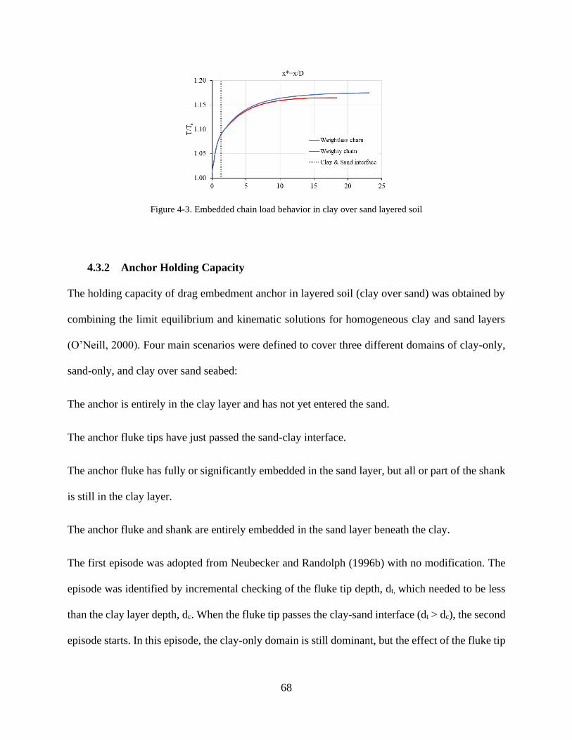
68
Figure 4-3. Embedded chain load behavior in clay over sand layered soil
4.3.2 Anchor Holding Capacity
The holding capacity of drag embedment anchor in layered soil (clay over sand) was obtained by
combining the limit equilibrium and kinematic solutions for homogeneous clay and sand layers
(O’Neill, 2000). Four main scenarios were defined to cover three different domains of clay-only,
sand-only, and clay over sand seabed:
The anchor is entirely in the clay layer and has not yet entered the sand.
The anchor fluke tips have just passed the sand-clay interface.
The anchor fluke has fully or significantly embedded in the sand layer, but all or part of the shank
is still in the clay layer.
The anchor fluke and shank are entirely embedded in the sand layer beneath the clay.
The first episode was adopted from Neubecker and Randolph (1996b) with no modification. The
episode was identified by incremental checking of the fluke tip depth, dt, which needed to be less
than the clay layer depth, dc. When the fluke tip passes the clay-sand interface (dt > dc), the second
episode starts. In this episode, the clay-only domain is still dominant, but the effect of the fluke tip
69
encountered with the sand layer was considered. O’Neill (2000) proposed the following equation
for calculation of fluke tip force that was added to Ta to obtain the revised anchor capacity, Ta:
𝐹𝑡 = 𝐴𝑡𝑞𝑠𝑎𝑛𝑑𝑁𝑡 (4-7)
where At is the projected area of fluke tips on a perpendicular plane to moving direction, qsand is
the standard sand strength, and Nt is bearing factor of fluke tip in the sand. The direction of Ft
assumed to be parallel to the direction of movement.
The standard sand strength, qsand, was obtained by:
𝑞𝑠𝑎𝑛𝑑 = 𝑐 𝑑𝑐 +
𝑠 (𝑑𝑡 − 𝑑𝑐) (4-8)
As the anchor embeds further in the seabed, it reaches a point which the dominant mechanism
changes to sand. The exact position of transition point is not well known; nevertheless, O’Neill
(2000) proposed, as the bottom depth of front shank face, dsf, transcends depth of clay-sand
interface, dc, the governing mechanism changes to sand-dominant behavior. Modifications were
done to the sand-dominant mechanism to use in this episode: first, adding the normal and shear
forces of clay on the fluke and shank, second, incorporating the clay overburden pressure. Figure
4-4 shows the modified acting forces on a drag anchor which has the sand-dominant mechanism.
Figure 4-4. Force system of anchor-soil in clay over sand
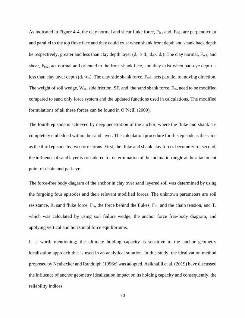
70
As indicated in Figure 4-4, the clay normal and shear fluke force, Ffc1 and, Ffc2, are perpendicular
and parallel to the top fluke face and they could exist when shank front depth and shank back depth
be respectively, greater and less than clay depth layer (dsf dc, dsb dc). The clay normal, Fsc1, and
shear, Fsc2, act normal and oriented to the front shank face, and they exist when pad-eye depth is
less than clay layer depth (da<dc). The clay side shank force, Fsc3, acts parallel to moving direction.
The weight of soil wedge, Wsc, side friction, SF, and, the sand shank force, Fss, need to be modified
compared to sand only force system and the updated functions used in calculations. The modified
formulations of all these forces can be found in O’Neill (2000).
The fourth episode is achieved by deep penetration of the anchor, where the fluke and shank are
completely embedded within the sand layer. The calculation procedure for this episode is the same
as the third episode by two corrections. First, the fluke and shank clay forces become zero; second,
the influence of sand layer is considered for determination of the inclination angle at the attachment
point of chain and pad-eye.
The force-free body diagram of the anchor in clay over sand layered soil was determined by using
the forgoing four episodes and their relevant modified forces. The unknown parameters are soil
resistance, R, sand fluke force, Ffs, the force behind the flukes, Ffb, and the chain tension, and Ta
which was calculated by using soil failure wedge, the anchor force free-body diagram, and
applying vertical and horizontal force equilibriums.
It is worth mentioning; the ultimate holding capacity is sensitive to the anchor geometry
idealization approach that is used in an analytical solution. In this study, the idealization method
proposed by Neubecker and Randolph (1996c) was adopted. Aslkhalili et al. (2019) have discussed
the influence of anchor geometry idealization impact on its holding capacity and consequently, the
reliability indices.
71
The anchor embedment trajectory in the layered soil (clay over sand) was obtained by using the
methodology proposed by Neubecker and Randolph (1996a) and extended by O’Neill et al. (1997).
The adopted methodology has been developed based on a minimum work approach. The anchor,
at some point in the soil with ultimate forces acting on it needs a certain amount of work to be
translated and rotated to some new geometry in the soil. A series of assumed displacements and
rotations are automatically tried to obtain the incremental relocation dissipating the least amount
of work. The corresponding displacement increment with the least dissipated energy is assumed
to be the anchor trajectory with the least resistance against the anchor relocation. More details of
the proposed kinematic model for the layered soil (clay over sand) could be found in Neubecker
and Randolph (1996a) and O’Neill (2000).
4.3.3 Developing Calculation Spreadsheet
The ultimate holding capacity and the trajectory of the anchor-chain system was calculated by
developing an Excel spreadsheet equipped with VBA macros. Figure 4-5 shows the iterative
calculation flowchart.
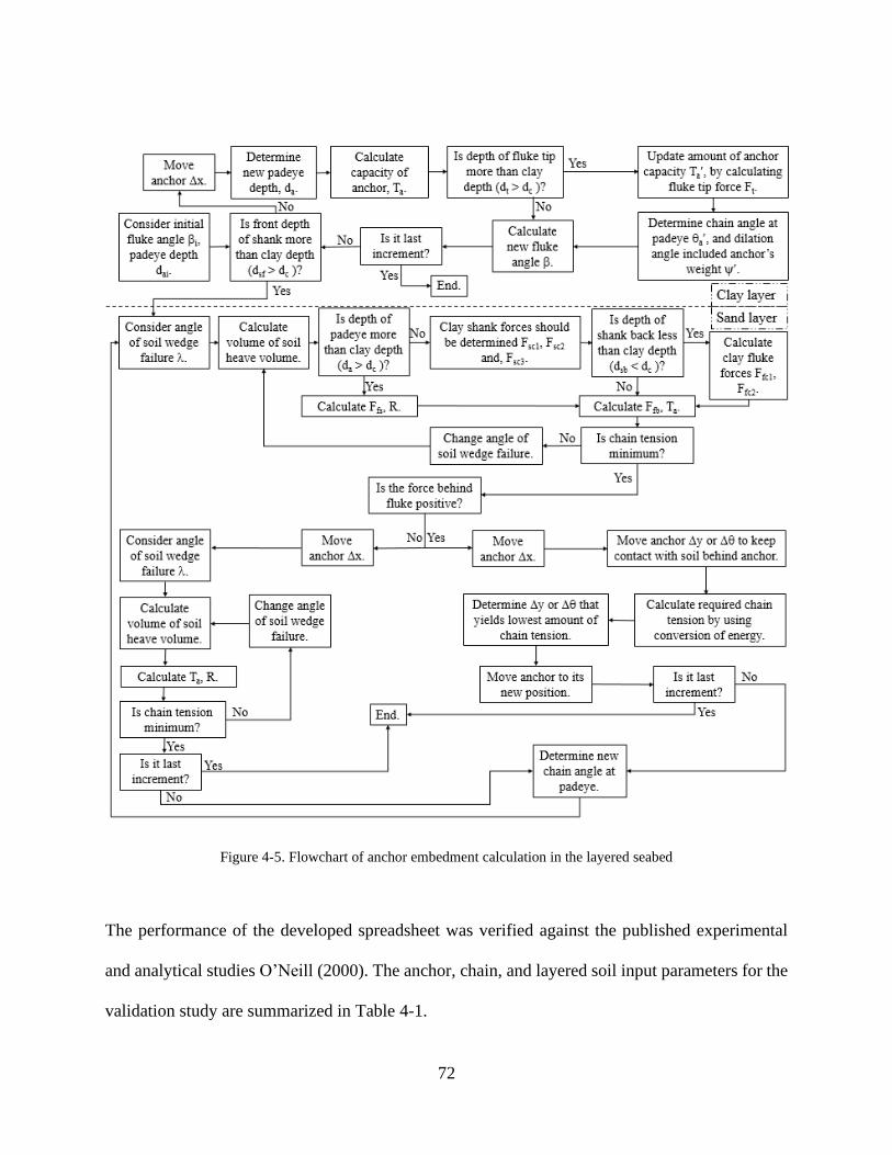
72
Figure 4-5. Flowchart of anchor embedment calculation in the layered seabed
The performance of the developed spreadsheet was verified against the published experimental
and analytical studies O’Neill (2000). The anchor, chain, and layered soil input parameters for the
validation study are summarized in Table 4-1.

73
Table 4-1. Soil and anchor input parameters in the current analysis
Figure 4-6 shows a perfect agreement between the developed spreadsheet and the existing
experimental and analytical studies.
Parameter Value
Anchor dry weight, Wa (kN) 313.6
Fluke length, Lf (m) 4.97
Fluke width, bf (m) 4.23
Fluke thickness, df (m) 0.72
Shank length, Ls (m) 8.07
Shank width, bs (m) 0.83
Fluke-Shank angle, fs () 27.1
Effective chain width, bc (m) 0.24
Chain self-weight, wc (kN/m) 2
Chain soil friction coefficient 0.4
Peak friction angle, p () 35
Shank bearing factor, Nqs 20
Dilation angle, () 8.5
Effective unit weight, s (kN/m3) 10
Fluke tip bearing factor, Nt 0.1
Surface undrained shear strength, su0 (kPa) 0
Undrained shear strength gradient,
sug(kPa/m)
1.5
Effective clay unit weight, c (kN/m3) 7.19
Clay bearing capacity factor, Nc 9
Clay layer depth, dc (m) 5.31

74
Figure 4-6. Comparison between anchor efficiency results
4.3.4 Anchors Selected for Reliability Studies
Stevpris Mk5 and Mk6 were used for reliability analysis in the current study. These anchors are
widely used for permanent and temporary station keeping of floating systems. Also, the selection
of these anchors enabled an effective comparison of the reliability results with earlier studies
conducted in homogenous clay and sand (Moharrami and Shiri (2018) and Aslkhalili et al. (2019)).
The ratio of fluke length to fluke thickness (Lf/df) in these anchors are 6.67 and 3.09 for Mk5 and
Mk6, respectively. Figure 4-7 indicates the plan and side view of these anchors with geometrical
properties given in Table 4-2.
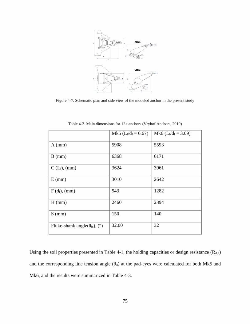
75
Figure 4-7. Schematic plan and side view of the modeled anchor in the present study
Table 4-2. Main dimensions for 12 t anchors (Vryhof Anchors, 2010)
Mk5 (Lf/df = 6.67) Mk6 (Lf/df = 3.09)
A (mm) 5908 5593
B (mm) 6368 6171
C (Lf), (mm) 3624 3961
E (mm) 3010 2642
F (df), (mm) 543 1282
H (mm) 2460 2394
S (mm) 150 140
Fluke-shank angle(θfs), () 32.00 32
Using the soil properties presented in Table 4-1, the holding capacities or design resistance (Rd,a)
and the corresponding line tension angle (a) at the pad-eyes were calculated for both Mk5 and
Mk6, and the results were summarized in Table 4-3.
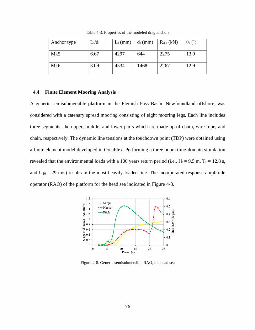
76
Table 4-3. Properties of the modeled drag anchors
Anchor type Lf/df Lf (mm) df (mm) Rd,a (kN) θa (˚)
Mk5 6.67 4297 644 2275 13.0
Mk6 3.09 4534 1468 2267 12.9
4.4 Finite Element Mooring Analysis
A generic semisubmersible platform in the Flemish Pass Basin, Newfoundland offshore, was
considered with a catenary spread mooring consisting of eight mooring legs. Each line includes
three segments; the upper, middle, and lower parts which are made up of chain, wire rope, and
chain, respectively. The dynamic line tensions at the touchdown point (TDP) were obtained using
a finite element model developed in OrcaFlex. Performing a three hours time-domain simulation
revealed that the environmental loads with a 100 years return period (i.e., Hs = 9.5 m, TP = 12.8 s,
and U10 = 29 m/s) results in the most heavily loaded line. The incorporated response amplitude
operator (RAO) of the platform for the head sea indicated in Figure 4-8.
Figure 4-8. Generic semisubmersible RAO, the head sea
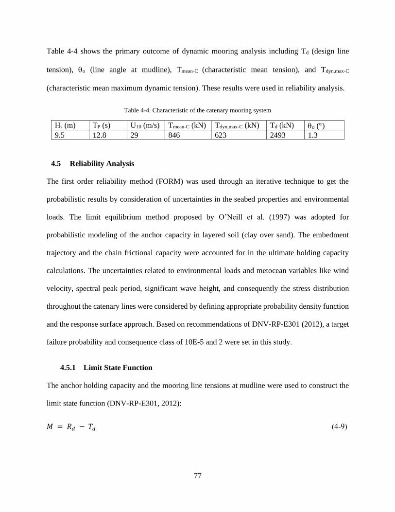
77
Table 4-4 shows the primary outcome of dynamic mooring analysis including Td (design line
tension), o (line angle at mudline), Tmean-C (characteristic mean tension), and Tdyn,max-C
(characteristic mean maximum dynamic tension). These results were used in reliability analysis.
Table 4-4. Characteristic of the catenary mooring system
Hs (m) TP (s) U10 (m/s) Tmean-C (kN) Tdyn,max-C (kN) Td (kN) o ()
9.5 12.8 29 846 623 2493 1.3
4.5 Reliability Analysis
The first order reliability method (FORM) was used through an iterative technique to get the
probabilistic results by consideration of uncertainties in the seabed properties and environmental
loads. The limit equilibrium method proposed by O’Neill et al. (1997) was adopted for
probabilistic modeling of the anchor capacity in layered soil (clay over sand). The embedment
trajectory and the chain frictional capacity were accounted for in the ultimate holding capacity
calculations. The uncertainties related to environmental loads and metocean variables like wind
velocity, spectral peak period, significant wave height, and consequently the stress distribution
throughout the catenary lines were considered by defining appropriate probability density function
and the response surface approach. Based on recommendations of DNV-RP-E301 (2012), a target
failure probability and consequence class of 10E-5 and 2 were set in this study.
4.5.1 Limit State Function
The anchor holding capacity and the mooring line tensions at mudline were used to construct the
limit state function (DNV-RP-E301, 2012):
𝑀 = 𝑅𝑑 − 𝑇𝑑 (4-9)

78
where Td and Rd are the design line tension and design anchor and chain system capacity at
mudline, respectively. The design line tension, Td, was formulated as the sum of the characteristic
mean line tension, Tmean-C, and the characteristic dynamic line tension, Tdyn,max-C. The characteristic
mean line tension, Tmean-C, is the result of the line pretension and mean environmental loads. The
maximum dynamic line tension, Tdyn,max-C, is representing the low-frequency and wave-frequency
vessel motions. The dynamic and characteristic mean line tensions were multiplied by relevant
partial safety factors, γdyn and γmean, respectively.
𝑇𝑑 = 𝑇𝑚𝑒𝑎𝑛−𝐶 ∙ 𝛾𝑚𝑒𝑎𝑛 + 𝑇𝑑𝑦𝑛−𝐶 ∙ 𝛾𝑑𝑦𝑛 (4-10)
The partial safety factors for mean and dynamic line tension was taken as 1.4 and 2.1 for
consequence class 2 (DNV-RP-E301, 2012). The significant wave height (Hs), peak period (Tp),
and wind velocity (U10) were used as primary parameters of the extreme sea-state. Both Tmean-C
and Tdyn,max-C were expressed as a function of those parameters at the mudline; therefore, the limit
state function can be written as:
𝑀 (𝑅, 𝐻𝑠, 𝑇𝑝, 𝑈10) = 𝑅𝑑 − 𝑇𝑚𝑒𝑎𝑛−𝐶 ∙ 𝛾𝑚𝑒𝑎𝑛 − 𝑇𝑑𝑦𝑛,𝑚𝑎𝑥−𝐶 ∙ 𝛾𝑑𝑦𝑛 (4-11)
The failure probability pF for a given extreme sea state was defined as:
𝑝𝐹 = 𝑃[𝑀 (𝑅, 𝐻𝑠, 𝑇𝑝, 𝑈10) ≤ 0] (4-12)
The annual probability of failure (pFa) for the incidence of extreme sea states was defined by
adopting a Poisson model and using an exponential function of failure probability (pF) (Silva-
González et al., 2013):
𝑝𝐹𝑎 = 1 − 𝑒𝑥𝑝(−𝜆𝑝𝐹) (4-13)
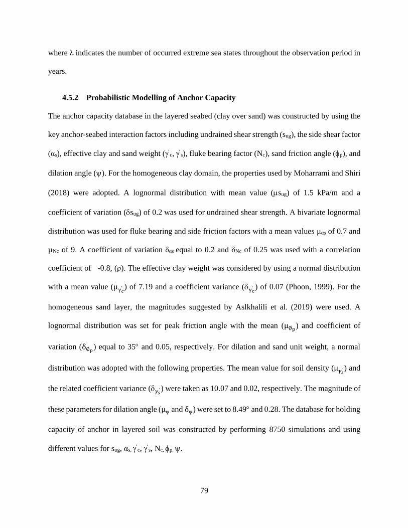
79
where λ indicates the number of occurred extreme sea states throughout the observation period in
years.
4.5.2 Probabilistic Modelling of Anchor Capacity
The anchor capacity database in the layered seabed (clay over sand) was constructed by using the
key anchor-seabed interaction factors including undrained shear strength (sug), the side shear factor
(αs), effective clay and sand weight (c, s), fluke bearing factor (Nc), sand friction angle (p), and
dilation angle (). For the homogeneous clay domain, the properties used by Moharrami and Shiri
(2018) were adopted. A lognormal distribution with mean value (sug) of 1.5 kPa/m and a
coefficient of variation (sug) of 0.2 was used for undrained shear strength. A bivariate lognormal
distribution was used for fluke bearing and side friction factors with a mean values μαs of 0.7 and
µNc of 9. A coefficient of variation δαs equal to 0.2 and δNc of 0.25 was used with a correlation
coefficient of -0.8, (ρ). The effective clay weight was considered by using a normal distribution
with a mean value (μγc ) of 7.19 and a coefficient variance (γc
) of 0.07 (Phoon, 1999). For the
homogeneous sand layer, the magnitudes suggested by Aslkhalili et al. (2019) were used. A
lognormal distribution was set for peak friction angle with the mean (μ∅p) and coefficient of
variation (δ∅p) equal to 35 and 0.05, respectively. For dilation and sand unit weight, a normal
distribution was adopted with the following properties. The mean value for soil density (μ𝛾𝑠 ) and
the related coefficient variance (𝛾𝑠 ) were taken as 10.07 and 0.02, respectively. The magnitude of
these parameters for dilation angle (μ and δ) were set to 8.49 and 0.28. The database for holding
capacity of anchor in layered soil was constructed by performing 8750 simulations and using
different values for sug, αs, c, s, Nc, p, .
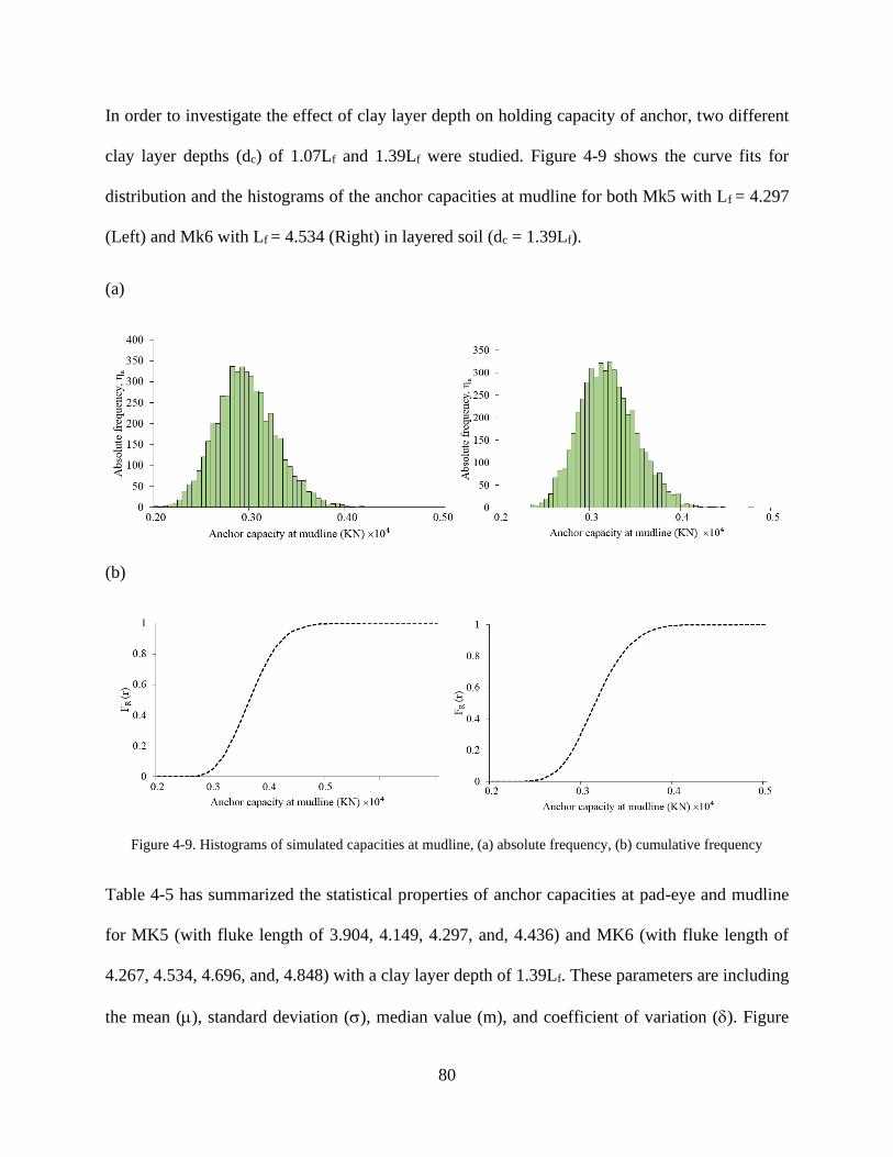
80
In order to investigate the effect of clay layer depth on holding capacity of anchor, two different
clay layer depths (dc) of 1.07Lf and 1.39Lf were studied. Figure 4-9 shows the curve fits for
distribution and the histograms of the anchor capacities at mudline for both Mk5 with Lf = 4.297
(Left) and Mk6 with Lf = 4.534 (Right) in layered soil (dc = 1.39Lf).
(a)
(b)
Figure 4-9. Histograms of simulated capacities at mudline, (a) absolute frequency, (b) cumulative frequency
Table 4-5 has summarized the statistical properties of anchor capacities at pad-eye and mudline
for MK5 (with fluke length of 3.904, 4.149, 4.297, and, 4.436) and MK6 (with fluke length of
4.267, 4.534, 4.696, and, 4.848) with a clay layer depth of 1.39Lf. These parameters are including
the mean (), standard deviation (), median value (m), and coefficient of variation (). Figure

81
4-10 shows the variation of the mean and standard deviation of anchor capacity at pad-eye and
mudline against the fluke length for MK6 anchor family in two different clay layer depth
(dc=1.07Lf and 1.39Lf).
Table 4-5. Statistical properties of anchor capacity at pad-eye and mudline
Model Lf/df Lf (m) Padeye Mudline µRa/µR
µRa
(kN)
σRa
(kN)
δRa mRa
(kN)
µR
(kN)
σR
(kN)
δR mR
(kN)
MK5 6.67 3.904 2672.6 309.87 0.115 2646.0 2847.2 331.26 0.1163 2809.0 0.93
MK5 6.67 4.149 3127.3 360.30 0.115 3080.0 3312.4 396.29 0.1196 3263.0 0.94
MK5 6.67 4.297 3472.0 426.97 0.122 3403.0 3674.4 446.85 0.1216 3600.0 0.94
MK5 6.67 4.436 3772.6 456.76 0.121 3709.5 3988.2 480.92 0.1205 3922.5 0.94
MK6 3.09 4.267 3082.5 360.77 0.117 3022.5 3294.6 376.08 0.1141 3218.5 0.93
MK6 3.09 4.534 3684.3 399.84 0.108 3624.0 3914.0 423.45 0.1081 3852.0 0.94
MK6 3.09 4.696 4106.2 493.49 0.120 4025.5 4356.9 522.16 0.1198 4275.0 0.94
MK6 3.09 4.848 4507.4 516.49 0.114 4426.0 4777.0 546.03 0.1143 4695.0 0.94
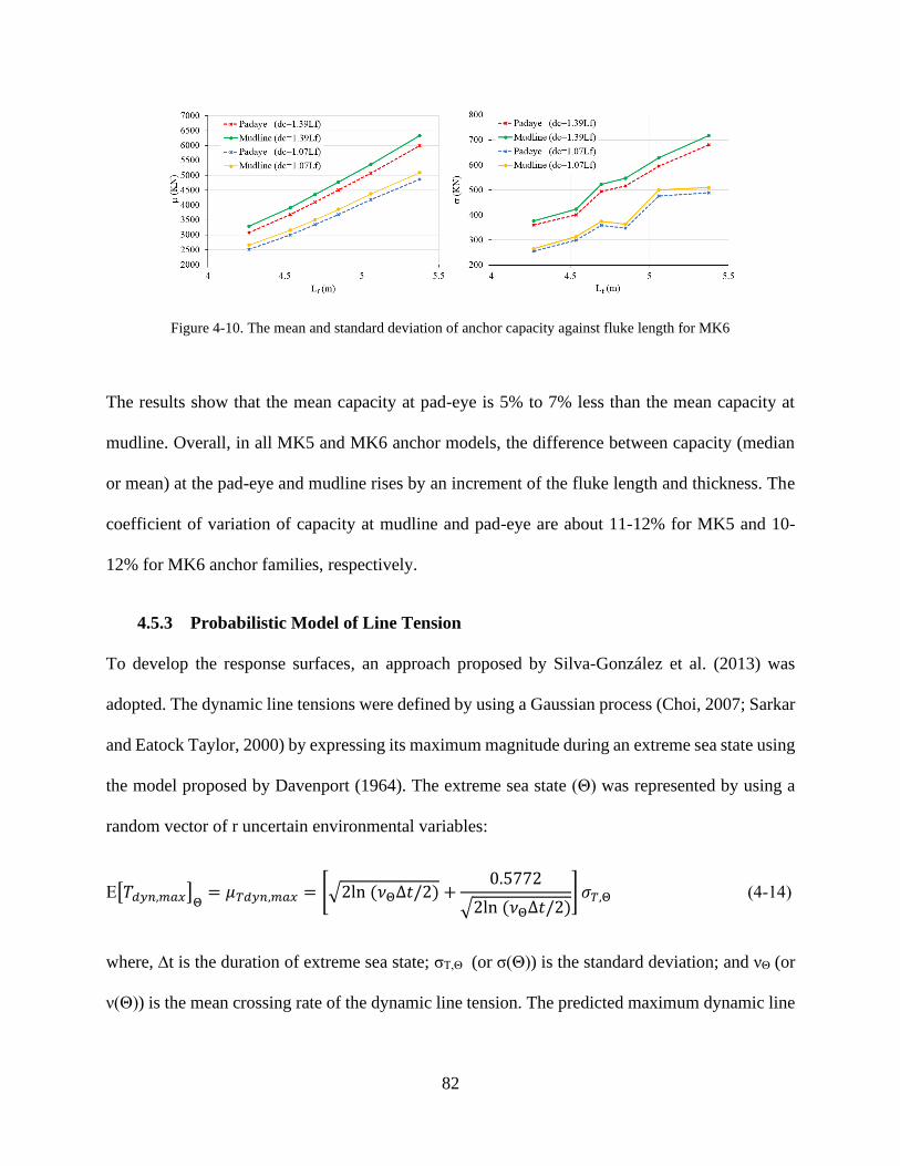
82
Figure 4-10. The mean and standard deviation of anchor capacity against fluke length for MK6
The results show that the mean capacity at pad-eye is 5% to 7% less than the mean capacity at
mudline. Overall, in all MK5 and MK6 anchor models, the difference between capacity (median
or mean) at the pad-eye and mudline rises by an increment of the fluke length and thickness. The
coefficient of variation of capacity at mudline and pad-eye are about 11-12% for MK5 and 10-
12% for MK6 anchor families, respectively.
4.5.3 Probabilistic Model of Line Tension
To develop the response surfaces, an approach proposed by Silva-González et al. (2013) was
adopted. The dynamic line tensions were defined by using a Gaussian process (Choi, 2007; Sarkar
and Eatock Taylor, 2000) by expressing its maximum magnitude during an extreme sea state using
the model proposed by Davenport (1964). The extreme sea state (Θ) was represented by using a
random vector of r uncertain environmental variables:
E[𝑇𝑑𝑦𝑛,𝑚𝑎𝑥]Θ
= 𝜇𝑇𝑑𝑦𝑛,𝑚𝑎𝑥 = [√2ln (𝜈ΘΔ𝑡/2) +0.5772
√2ln (𝜈ΘΔ𝑡/2)] 𝜎𝑇,Θ (4-14)
where, ∆t is the duration of extreme sea state; σT,Θ (or σ(Θ)) is the standard deviation; and νΘ (or
ν(Θ)) is the mean crossing rate of the dynamic line tension. The predicted maximum dynamic line
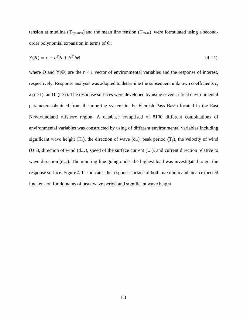
83
tension at mudline (Tdyn,max) and the mean line tension (Tmean) were formulated using a second-
order polynomial expansion in terms of Θ:
𝑌(𝛩) = 𝑐 + 𝑎𝑇𝛩 + 𝛩𝑇𝑏𝛩 (4-15)
where Θ and Y(Θ) are the r × 1 vector of environmental variables and the response of interest,
respectively. Response analysis was adopted to determine the subsequent unknown coefficients c,
a (r ×1), and b (r ×r). The response surfaces were developed by using seven critical environmental
parameters obtained from the mooring system in the Flemish Pass Basin located in the East
Newfoundland offshore region. A database comprised of 8100 different combinations of
environmental variables was constructed by using of different environmental variables including
significant wave height (Hs), the direction of wave (dw), peak period (Tp), the velocity of wind
(U10), direction of wind (dww), speed of the surface current (Uc), and current direction relative to
wave direction (dwc). The mooring line going under the highest load was investigated to get the
response surface. Figure 4-11 indicates the response surface of both maximum and mean expected
line tension for domains of peak wave period and significant wave height.
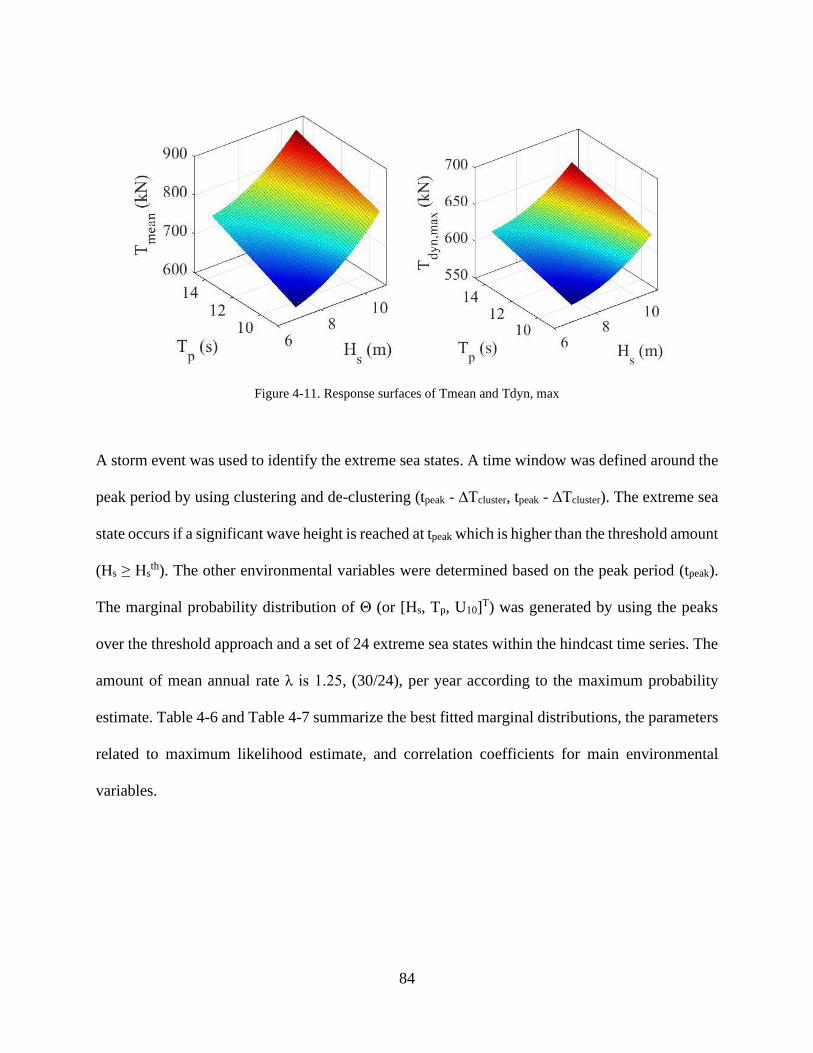
84
Figure 4-11. Response surfaces of Tmean and Tdyn, max
A storm event was used to identify the extreme sea states. A time window was defined around the
peak period by using clustering and de-clustering (tpeak - ∆Tcluster, tpeak - ∆Tcluster). The extreme sea
state occurs if a significant wave height is reached at tpeak which is higher than the threshold amount
(Hs ≥ Hsth). The other environmental variables were determined based on the peak period (tpeak).
The marginal probability distribution of Θ (or [Hs, Tp, U10]T) was generated by using the peaks
over the threshold approach and a set of 24 extreme sea states within the hindcast time series. The
amount of mean annual rate λ is 1.25, (30/24), per year according to the maximum probability
estimate. Table 4-6 and Table 4-7 summarize the best fitted marginal distributions, the parameters
related to maximum likelihood estimate, and correlation coefficients for main environmental
variables.
85
Table 4-6. Distribution parameters of environmental variables
Variable Probability distribution Distribution parameters
Hs Weibull Scale 9.5351
Shape 10.1552
Tp Lognormal µlnTp 2.4966
σlnTp 0.1196
U10 Lognormal µlnU10 3.4827
σlnU10 0.1095
Table 4-7. Estimated correlation coefficients
Hs Tp U10
Hs 1.0 0.9728 0.9905
Tp 0.9728 1.0 0.9935
U10 0.9905 0.9935 1.0
4.5.4 Results of Reliability Analysis
Figure 4-12 illustrates the variation of annual reliability index versus fluke length (plot a) and dry
anchor weight (plot b) in two different clay layer depth (1.07Lf, 1.39Lf). Each point on plot A
linked to an equivalent point on plot B and vice versa. For instance, in both plots of Figure 4-12,
point 3 represents an MK6 anchor with a length of 4.696 m and a weight of 20 t in clay layer depth
of 1.39Lf with an annual reliability index of 4.89.
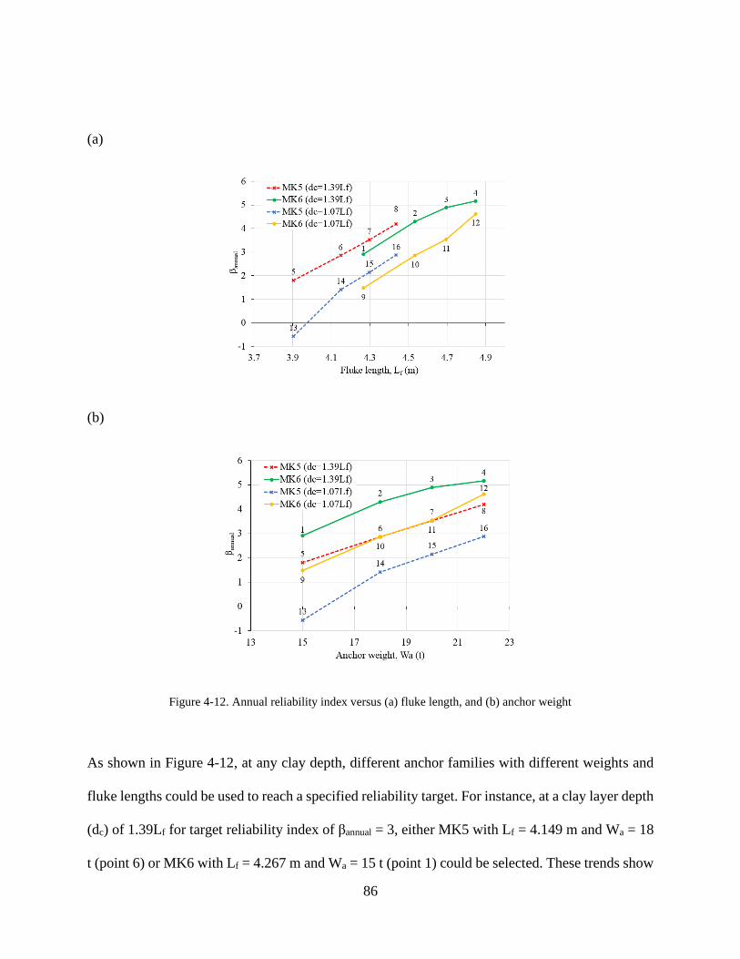
86
(a)
(b)
Figure 4-12. Annual reliability index versus (a) fluke length, and (b) anchor weight
As shown in Figure 4-12, at any clay depth, different anchor families with different weights and
fluke lengths could be used to reach a specified reliability target. For instance, at a clay layer depth
(dc) of 1.39Lf for target reliability index of βannual = 3, either MK5 with Lf = 4.149 m and Wa = 18
t (point 6) or MK6 with Lf = 4.267 m and Wa = 15 t (point 1) could be selected. These trends show

87
that same as homogeneous clay (Moharrami and Shiri, 2018), anchors with different weights, but
identical fluke lengths produce very close reliability levels. For achieving target failure
probabilities between 10-4 and 10-5 (with dc=1.39Lf), the existing weight and fluke length for MK5
is 22 t and 4.436 m and for MK6 is 18 t and 4.534 m. The mentioned target failure probabilities
are generally used as the ultimate limit state design in offshore systems (DNV-OS-E-301 2010;
DNV-OS-F201, 2010; DNVGL-ST-F101, 2019). Also, at a given clay layer depth, two different
anchor families with the same weight and different fluke length result in different annual reliability
indices. For a weight of 15 t (with dc=1.39Lf) by changing fluke length from 3.904 m (point 5) in
MK5 to 4.267 m (point 1) in MK6, the annual reliability index increases from 1.80 to 2.91 which
corresponds to a reduction of annual failure probability by one order of magnitude from 0.0355 to
0.0018. Similar to homogeneous clay condition (Moharrami and Shiri, 2018), the capacity of
deeply embedded anchors in layered soil (clay over sand) is significantly affected by fluke length,
while the anchor weight is not a significant factor. In each anchor family, the annual reliability
index increases when the clay layer depth increases. For instance, the annual reliability index of
an MK5 anchor with a fluke length of 4.297 m increases from 2.15 to 3.532 when clay layer depth
(dc) increases from 1.07Lf to 1.39Lf.
The logarithmic variation of failure probability (log (PFa)) against anchor weight and fluke length
with their linear curve fit in two different clay layer depth (dc) for MK5 and MK6 anchor families
are shown in Figure 4-13.
(a)
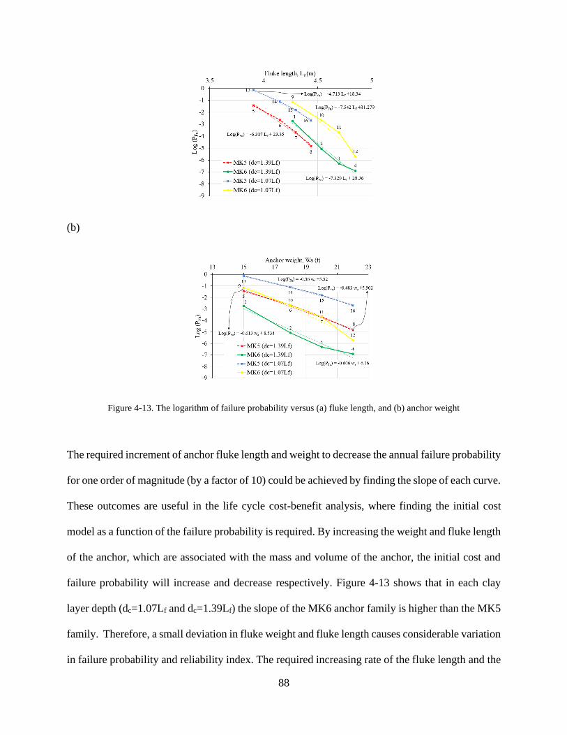
88
(b)
Figure 4-13. The logarithm of failure probability versus (a) fluke length, and (b) anchor weight
The required increment of anchor fluke length and weight to decrease the annual failure probability
for one order of magnitude (by a factor of 10) could be achieved by finding the slope of each curve.
These outcomes are useful in the life cycle cost-benefit analysis, where finding the initial cost
model as a function of the failure probability is required. By increasing the weight and fluke length
of the anchor, which are associated with the mass and volume of the anchor, the initial cost and
failure probability will increase and decrease respectively. Figure 4-13 shows that in each clay
layer depth (dc=1.07Lf and dc=1.39Lf) the slope of the MK6 anchor family is higher than the MK5
family. Therefore, a small deviation in fluke weight and fluke length causes considerable variation
in failure probability and reliability index. The required increasing rate of the fluke length and the
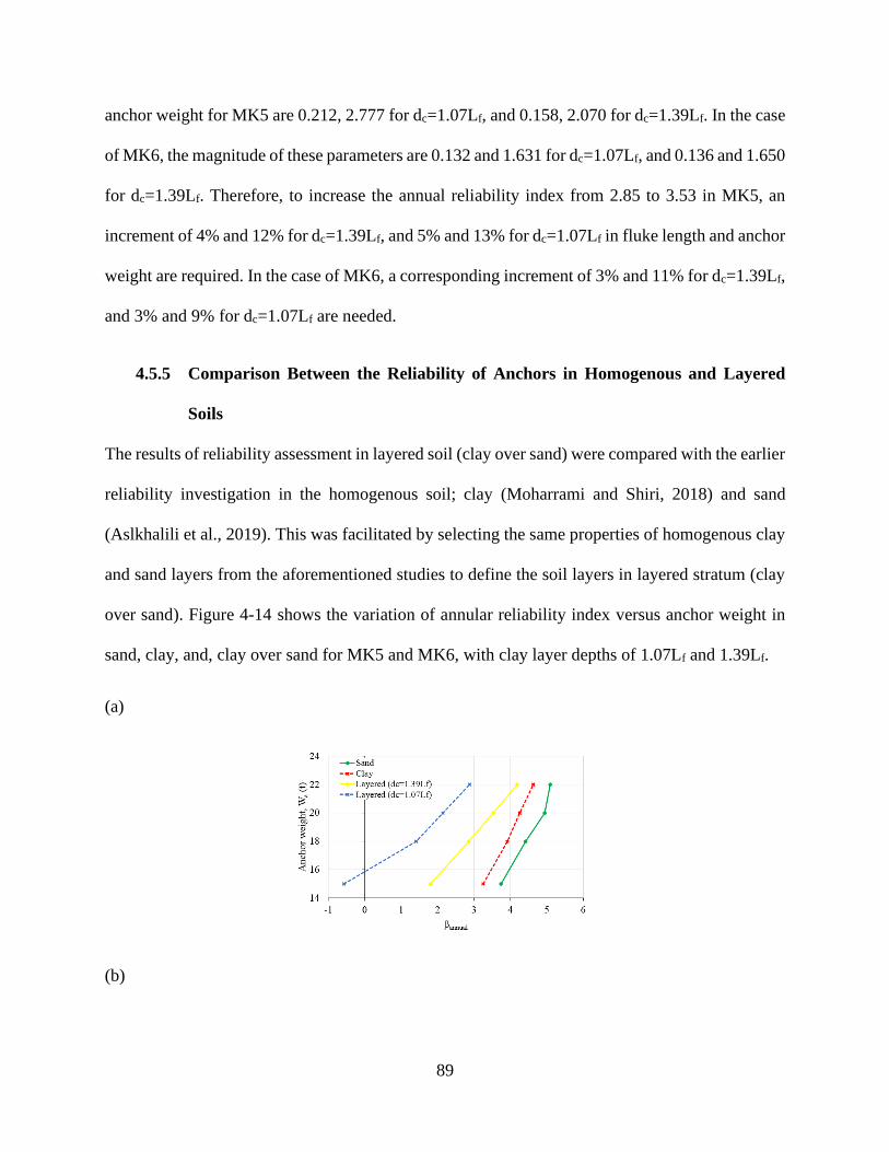
89
anchor weight for MK5 are 0.212, 2.777 for dc=1.07Lf, and 0.158, 2.070 for dc=1.39Lf. In the case
of MK6, the magnitude of these parameters are 0.132 and 1.631 for dc=1.07Lf, and 0.136 and 1.650
for dc=1.39Lf. Therefore, to increase the annual reliability index from 2.85 to 3.53 in MK5, an
increment of 4% and 12% for dc=1.39Lf, and 5% and 13% for dc=1.07Lf in fluke length and anchor
weight are required. In the case of MK6, a corresponding increment of 3% and 11% for dc=1.39Lf,
and 3% and 9% for dc=1.07Lf are needed.
4.5.5 Comparison Between the Reliability of Anchors in Homogenous and Layered
Soils
The results of reliability assessment in layered soil (clay over sand) were compared with the earlier
reliability investigation in the homogenous soil; clay (Moharrami and Shiri, 2018) and sand
(Aslkhalili et al., 2019). This was facilitated by selecting the same properties of homogenous clay
and sand layers from the aforementioned studies to define the soil layers in layered stratum (clay
over sand). Figure 4-14 shows the variation of annular reliability index versus anchor weight in
sand, clay, and, clay over sand for MK5 and MK6, with clay layer depths of 1.07Lf and 1.39Lf.
(a)
(b)
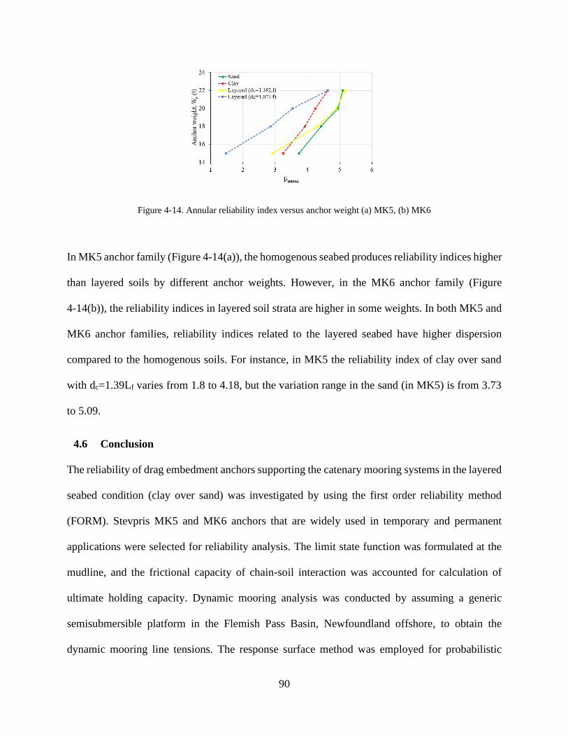
90
Figure 4-14. Annular reliability index versus anchor weight (a) MK5, (b) MK6
In MK5 anchor family (Figure 4-14(a)), the homogenous seabed produces reliability indices higher
than layered soils by different anchor weights. However, in the MK6 anchor family (Figure
4-14(b)), the reliability indices in layered soil strata are higher in some weights. In both MK5 and
MK6 anchor families, reliability indices related to the layered seabed have higher dispersion
compared to the homogenous soils. For instance, in MK5 the reliability index of clay over sand
with dc=1.39Lf varies from 1.8 to 4.18, but the variation range in the sand (in MK5) is from 3.73
to 5.09.
4.6 Conclusion
The reliability of drag embedment anchors supporting the catenary mooring systems in the layered
seabed condition (clay over sand) was investigated by using the first order reliability method
(FORM). Stevpris MK5 and MK6 anchors that are widely used in temporary and permanent
applications were selected for reliability analysis. The limit state function was formulated at the
mudline, and the frictional capacity of chain-soil interaction was accounted for calculation of
ultimate holding capacity. Dynamic mooring analysis was conducted by assuming a generic
semisubmersible platform in the Flemish Pass Basin, Newfoundland offshore, to obtain the
dynamic mooring line tensions. The response surface method was employed for probabilistic

91
modeling of the line tensions at the mudline. The ultimate holding capacity and the anchor
trajectory were calculated by developing an Excel spreadsheet integrated with VBA macros for
iterative analysis. The annual reliability indices and failure probabilities in layers soil strata were
obtained and compared with earlier studies in homogenous clay and sand layers. The primary
outcomes of the study are summarized as follow:
• The seabed soil stratum and its configuration (individual layer thickness) have a significant
influence on reliability indices. Overall, the probability of failure is higher for the layered
clay over sand stratum compared with homogeneous clay and sand layers. This suggests
that the recommended practices that are currently considering only homogeneous soil
should be re-assessed and possibly improved for complex, layered seabed soil strata.
• The geometrical anchor configuration, particularly the fluke length, was found to have a
significant effect on holding capacity and consequently the reliability indices. The anchor
weight showed a positive influence on reliability results, but less effective than the fluke
length. The geometrical improvement of the anchors can effectively improve their
reliability. In addition, the current design practice is identical for all of the different anchor
families. This approach does not account for the significant influence of anchor geometry
and the uncertainties associated with different anchor families, environmental, and
operational loads. The reliability-based refinement of the design procedure can
considerably improve the reliability and cost-effectiveness of anchor design.
• The configuration of layered soil strata, particularly the depth and thickness of layers
showed a significant effect on ultimate holding capacity and reliability indices. Thicker
clay layers resulted in higher reliability indices. Different range of layer thickness still
needs to be investigated to generalize the obtained results.

92
Although the analytical and numerical solutions are quite beneficial to assess the parameters
affecting the reliability of drag embedment anchors. However, the reliability assessment of anchors
can be significantly improved by having access to in-field test databases, related seabed properties,
and, statistical data of failures. The current study was limited to specific anchor families
performing in clay over sand seabed strata with two instances of layer thickness. Further
investigations are necessary for different layer configurations such as sand over clay, sand over
sand, and clay over the clay; and also different anchor families.
Acknowledgments
The authors gratefully acknowledge the financial support of this research by the Memorial
University of Newfoundland through VP start-up fund and school of graduate studies (SGS). The
technical advice of Mr. Mohammad Javad Moharrami and Mr. Rahim Shoughi is also kindly
acknowledged.
93
References
Aslkhalili, A., Shiri, H., Zendehboudi, S., 2019. Reliability assessment of drag embedment anchors
in sand and the effect of idealized anchor geometry. Saf. Extrem. Environ. 1, 39–57.
https://doi.org/10.1007/s42797-019-00006-5
Choi, Y.J., 2007. Reliability Assessment of Foundations for Offshore Mooring Systems under
Extreme Environments.
Clukey, E.C., Gilbert, R.B., Andersen, K.H., Dahlberg, R., 2013. Reliability of Suction Caissons
for Deep Water Floating Facilities 1991, 456–474.
https://doi.org/10.1061/9780784412763.035
Davenport, A.G., 1964. Note on the Distribution of the Largest Value of a Random Function With
Application To Gust Loading. Proc. Inst. Civ. Eng. 28, 187–196.
https://doi.org/10.1680/iicep.1964.10112
DNV-OS-E-301, 2010. Position Mooring. Offshore Standard.
DNV-OS-F201, 2010. Dynamic Risers. Offshore Standard.
DNV-RP-E301, 2012. Design and Installation of Fluke Anchors.
DNVGL-ST-F101, 2019. Submarine Pipeline Systems. Offshore standartd.
Duggal, A., Ma, K., Shu, H., Smedley, P., L'Hostis, D., 2013. A Historical Review on
Integrity Issues of Permanent Mooring Systems 3. https://doi.org/10.4043/24025-ms
Dunnavant, T.W., Kwan, C.-T.T., 1993. Centrifuge Modelling And Parametric Analyses Of Drag
Anchor Behavior, in: Offshore Technology Conference. https://doi.org/10.4043/7202-ms
Moharrami, M.J., Shiri, H., 2018. Reliability assessment of drag embedment anchors in clay for
94
catenary mooring systems. Mar. Struct. 58, 342–360.
https://doi.org/10.1016/j.marstruc.2017.12.005
Montes-Iturrizaga, R., Heredia-Zavoni, E., 2016. Reliability analysis of mooring lines using
copulas to model statistical dependence of environmental variables. Appl. Ocean Res. 59,
564–576. https://doi.org/10.1016/j.apor.2016.07.008
Neubecker, S.R., 1995. The behaviour of drag anchor and chain systems, PhD Thesis, Department
of Civil Engineering, The University of Western Australia.
Neubecker, S.R., Randolph, M.F., 1996a. The performance of drag anchor and chain systems in
cohesive soil. Georesources Geotech. 14, 1–7.
Neubecker, S.R., Randolph, M.F., 1996b. The kinematic behaviour of drag anchors in sand. Can.
Geotech. J. 33, 584–594. https://doi.org/https://doi.org/10.1139/t96-084-306
Neubecker, S.R., Randolph, M.F., 1996c. The static equilibrium of drag anchors in sand. Can.
Geotech. J. 33, 574–583.
Neubecker, S.R., Randolph, M.F., 1995a. Profile and frictional capacity of embedded anchor
chains. Geotech. Eng. 121, 797–803.
Neubecker, S.R., Randolph, M.F., 1995b. Performance of Embedded Anchor Chains and
Consequences for Anchor Design. https://doi.org/10.4043/7712-ms
O’Neill, M.P., 2000. The behaviour of drag anchors in layered soils, PhD Thesis, Department of
Civil Engineering, The University of Western Australia.
O’Neill, M.P., Bransby, M.F., Randolph, M.F., 2003. Drag anchor fluke–soil interaction in clays.
Can. Geotech. J. 40, 78–94. https://doi.org/10.1139/t02-096
95
O’Neill, M.P., Randolph, M.F., House, A.R., 1997. A preliminary assessment of the behaviour of
drag anchors in layered soils 9.
Phoon, K.K., 1999. Characterization of geotechnical variability. Can. Geotech. J. 624, 612–624.
Rendón-Conde, C., Heredia-Zavoni, E., 2016. Reliability analysis of suction caissons for moored
structures under parameter uncertainties. Struct. Saf. 60, 102–116.
https://doi.org/10.1016/j.strusafe.2016.02.004
Sarkar, A., Eatock Taylor, R., 2000. Effects of mooring line drag damping on response statistics
of vessels excited by first- and second-order wave forces. Ocean Eng. 27, 667–686.
https://doi.org/10.1016/S0029-8018(99)00014-1
Silva-González, F., Heredia-Zavoni, E., Valle-Molina, C., Sánchez-Moreno, J., Gilbert, R.B.,
2013. Reliabilitystudy of suction caissons for catenary and taut-leg mooring systems. Struct.
Saf. 45, 59–70. https://doi.org/10.1016/j.strusafe.2013.08.011
Valle-molina, C., Heredia-zavoni, E., Silva-gonzález, F.L., 2008. Reliability analyses of suction
caissons for FPSO systems, in: International Conference on Offshore Mechanics and Arctic
Engineering. pp. 1–6.
Vryhof Anchors, 2010. Anchor manual. Krimpen ad Yssel, The Netherlands.
96
Chapter 5. Probabilistic Assessment of Lateral Pipeline-Backfill-Trench
Interaction
Amin Aslkhalili1, Hodjat Shiri 1, Sohrab Zendehboudi2
1. Civil Engineering Dept., Faculty of Engineering and Applied Science, Memorial University of
Newfoundland, A1B 3X5, St. John’s, NL, Canada.
2. Process Engineering Dept., Faculty of Engineering and Applied Science, Memorial University
of Newfoundland, A1B 3X5, St. John’s, NL, Canada.
This chapter is currently under review as a journal manuscript

97
Abstract
In seismic regions, the buried pipelines may be at risk of fault displacement that applies massive
lateral pipe movements and jeopardizes the mechanical integrity of the buried pipes. Trenching
and the burial of pipelines is a common practice for physical protection. The lower stiffness of the
remoulded backfilling material relative to the native ground has a significant impact on lateral soil
resistance against large pipeline displacements that is rarely considered in the current design
practice. Finding a safe, reliable, and cost-effective trench configuration is a key aspect of design
practice that is affected by pipeline-backfill-trench interaction. In this analysis, a probabilistic
approach was employed to investigate the trenching/backfilling effect on the response of the buried
pipelines to large lateral displacements. A three-dimensional beam-spring model subjected to a
strike-slip fault was developed and the effect of trenching/backfilling was incorporated by using
non-linear springs. Two limit state criteria were set to identify the safe and failure regions. A
Python code was developed to perform iterative analysis by variation of pipe specifications, native
and backfill soil properties, trench width, trench depth, and lateral displacements. The first order
reliability method (FORM) was used to estimate the exceedance probability of failure by using the
identified limit states. The study showed that the trenching/backfilling of the pipeline results in
lower lateral soil resistance against the displaced pipe. Also, it was observed that the advantage of
load reduction could be used for mitigation of trench dimensions and reduction of the construction
costs without jeopardizing the safety and integrity requirements.
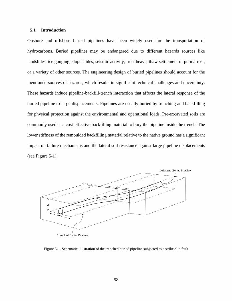
98
5.1 Introduction
Onshore and offshore buried pipelines have been widely used for the transportation of
hydrocarbons. Buried pipelines may be endangered due to different hazards sources like
landslides, ice gouging, slope slides, seismic activity, frost heave, thaw settlement of permafrost,
or a variety of other sources. The engineering design of buried pipelines should account for the
mentioned sources of hazards, which results in significant technical challenges and uncertainty.
These hazards induce pipeline-backfill-trench interaction that affects the lateral response of the
buried pipeline to large displacements. Pipelines are usually buried by trenching and backfilling
for physical protection against the environmental and operational loads. Pre-excavated soils are
commonly used as a cost-effective backfilling material to bury the pipeline inside the trench. The
lower stiffness of the remoulded backfilling material relative to the native ground has a significant
impact on failure mechanisms and the lateral soil resistance against large pipeline displacements
(see Figure 5-1).
Figure 5-1. Schematic illustration of the trenched buried pipeline subjected to a strike-slip fault

99
The trenching/backfilling effect is rarely considered in the current design codes (e.g., DNVGL-
RP-F114, 2017; PRCI, 2009; ALA, 2005; ASCE committee, 2014). The solutions that has been
proposed based on various earlier studies on lateral pipe-soil interaction (Tschebotarioff, 1973;
Wantland et al., 1979; Paulin, 1998) or anchor soil interactions (Hansen, 1948, Hansen and
Christensen, 1961; Smith, 1962; Ovesen, 1964; Kostyukov, 1963; Ovesen and Stroman, 1972;
Neely et al., 1973; Das and Seeley, 1975; Rowe and Davis, 1982; Merifield et al., 2001). However,
the number of studies considering the pipeline-backfill-trench interaction effect on lateral pipe
response is quite limited (Paulin, 1998; C-CORE, 2003, 2004, 2005; Phillips et al., 2004; Kianian
et al., 2018; Kianian and Shiri, 2019; Kianian and Shiri, 2020).
Considering a broad range of uncertainties affecting the pipeline response to large lateral
displacments, probabilistic design methods have been recently recommended by design codes
(e.g., DNVGL-ST-F101, 2019) as a reasonable and alternate design approach. There are a few
studies in the literature that has used probabilistic approaches to investigate this challenging area
of engineering (e.g., Nobahar et al., 2007; Cheng and Akkar, 2017). However, neither of these
studies have accounted for the uncertainties arising from the trenching/backfilling effects.
In this study, a probabilistic approach was utilized to study the mechanical integrity of buried
pipelines exposed to massive lateral soil displacement due to seismic fault movement in clay with
the incorporation of the trenching/backfilling effects. A 3D beam/spring finite element model was
developed in ABAQUS and the effect of trenching/backfilling was incorporated by non-linear later
spring extracted from the published centrifuge model tests (i.e., Paulin, 1998). Two different
pipeline failure envelopes were considered based on serviceability and ultimate limit state design
to identify failure zones and calculate failure probabilities. A Python code was developed for
iterative computations and performing the probabilistic assessment of the pipeline mechanical
100
integrity using the FORM. Different trench geometries, fault displacement, and pipe geometrical
properties were examined to obtain the annual failure probability and the corresponding trench
configurations. It should be mentioned that the angle of the pipe-fault intersection () assumed to
be zero as it causes the maximum stress-strain states throughout the pipeline and considers as the
worth case scenario.
5.2 Finite Element Model
The pipeline-soil interaction can be model by continuum and beam-spring models. Each approach
has its pros and cons. The continuum models produce more accurate results using high
computational resources. The beam-spring approach is more cost-effective and fairly accurate
which is more used in daily engineering practice. However, the beam-spring analysis decoupled
the soil interaction in three directions and does not account for some of the complex soil behaviors
such as dilatancy, stress path dependency, and rate effects. Depending on the objectives, either of
these approaches can be selected to produce the desired outputs.
In the current study, since the probabilistic analysis requires a large number of FE model runs, the
beam-spring approach was adapted for a cost-effective analysis with acceptable level of
accuracies.
A three-dimensional beam-spring finite element model was developed in ABAQUS to model the
pipeline-backfill-trench interaction in the probabilistic analysis using three-node quadratic PIPE32
elements. Each node of the pipeline element has six degrees of freedom (three displacements and
three rotations), and quadratic shape function was used to define pipe elements. Additionally, other
variables represent average hoop stress regarding the thin-wall pipeline theory. A total length of
1000 m, 762 mm pipeline was modeled with assuming a 100 m fault zone in the center (50 m on

101
both sides of the fault crossing). The length of the pipe was selected long enough to prevent the
boundary effects of the pipe ends, as suggested by earlier studies (Takada et al., 2001; Karamitros
et al., 2007).
Using mesh sensitivity analysis, the mesh size was selected to be 10 m throughout the pipe, and 1
m in the fault zone. The stress-strain constitutive relationship of the pipeline was identified by
isotropic, elastoplastic behavior with a von Mises yield surface, and isotropic hardening rule. The
stress-strain formulation proposed by Ramberg-Osgood was employed to define the stress-strain
relationship (Walker and Williams, 1995).
5.2.1 Pipe-Soil Model
Two-node nonlinear SPRINGA elements with hyperbolic responses were used in three directions
to model the elastoplastic soil interactions in axial, transverse horizontal, and transverse vertical
directions (see Figure 5-2).
Figure 5-2. Trenched buried pipe-soil interaction in a) continuum analysis, b) idealized structural model, and c) soil
load-displacement response curves in three directions
102
The induced seismic ground movements were applied as displacement boundary conditions to the
base of the soil spring elements. This simplified model is obtained from the subgrade reaction
concept initially proposed by Winkler (1867). In the beam-spring model, the soil resistance
function in each direction (axial 𝑡-𝑥, transverse horizontal 𝑝- 𝑦, and transverse vertical 𝑞- 𝑧)
defines the analytical expression which relates the maximum clay soil spring forces and
corresponding displacements. These resistance functions implicitly integrate the geomechanically
and geometrical properties of the pipeline-backfill trench interaction into the model.
A few lateral response of the trenched/backfilled pipelines in clay has been proposed in the
literature based on theoretical, numerical, and experimental studies (e.g., Paulin, 1998; C-CORE,
2003; Phillips et al., 2004; Kianian and Shiri, 2019; ASCE, 2005; PRCI, 2009). In the current
study, the pipeline-soil interaction model recommended by PRCI (2009) guideline was
incorporated.
5.2.2 Pipe Properties
The API 5L X65 grade material was chosen for the pipe. Three different nominal outside pipeline
diameter to wall thickness ratios (𝐷 𝑡⁄ ) were studied to represent the 𝐷 𝑡⁄ range that may be
employed in offshore pipeline designs (API, 2018). The pipeline parameters are presented in Table
5-1.
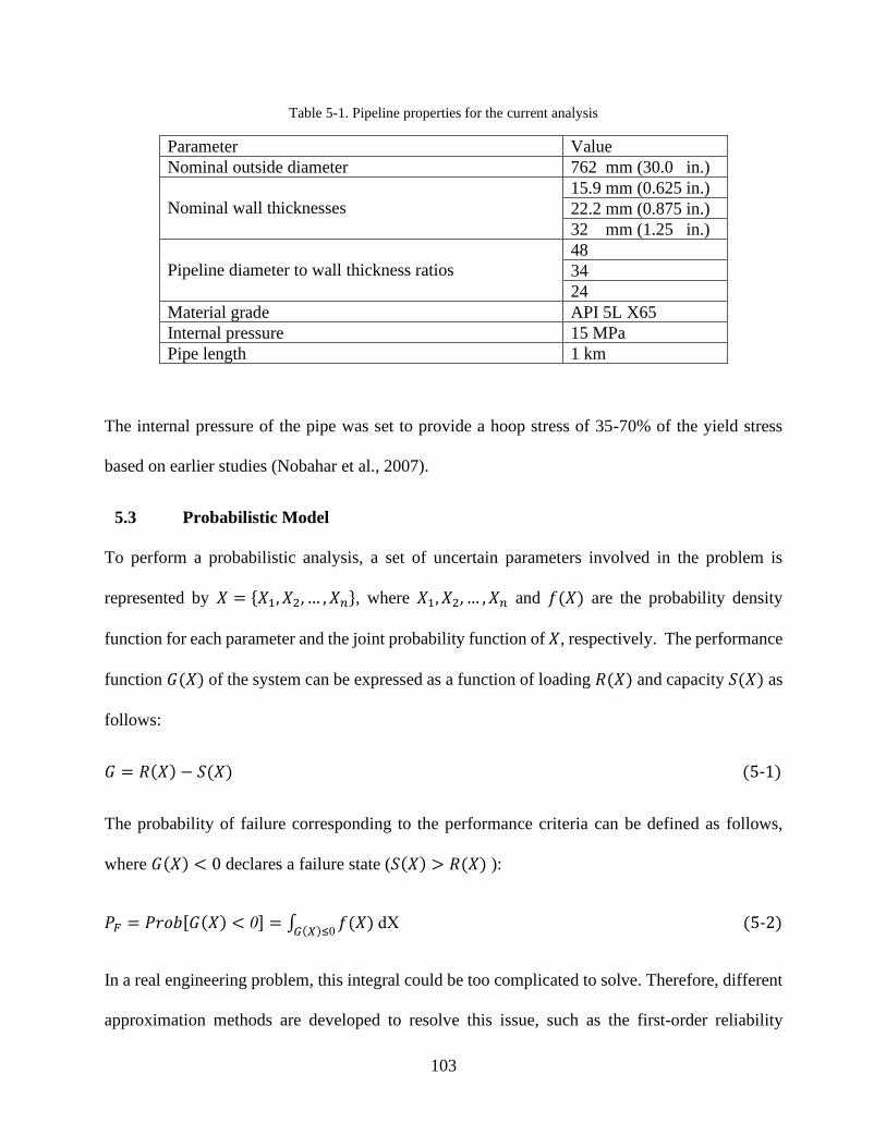
103
Table 5-1. Pipeline properties for the current analysis
Parameter Value
Nominal outside diameter 762 mm (30.0 in.)
Nominal wall thicknesses
15.9 mm (0.625 in.)
22.2 mm (0.875 in.)
32 mm (1.25 in.)
Pipeline diameter to wall thickness ratios
48
34
24
Material grade API 5L X65
Internal pressure 15 MPa
Pipe length 1 km
The internal pressure of the pipe was set to provide a hoop stress of 35-70% of the yield stress
based on earlier studies (Nobahar et al., 2007).
5.3 Probabilistic Model
To perform a probabilistic analysis, a set of uncertain parameters involved in the problem is
represented by 𝑋 = {𝑋1, 𝑋2, … , 𝑋𝑛}, where 𝑋1, 𝑋2, … , 𝑋𝑛 and 𝑓(𝑋) are the probability density
function for each parameter and the joint probability function of 𝑋, respectively. The performance
function 𝐺(𝑋) of the system can be expressed as a function of loading 𝑅(𝑋) and capacity 𝑆(𝑋) as
follows:
𝐺 = 𝑅(𝑋) − 𝑆(𝑋) (5-1)
The probability of failure corresponding to the performance criteria can be defined as follows,
where 𝐺(𝑋) < 0 declares a failure state (𝑆(𝑋) > 𝑅(𝑋) ):
𝑃𝐹 = 𝑃𝑟𝑜𝑏[𝐺(𝑋) < 0] = ∫ 𝑓(𝑋) dX𝐺(𝑋)≤0
(5-2)
In a real engineering problem, this integral could be too complicated to solve. Therefore, different
approximation methods are developed to resolve this issue, such as the first-order reliability
104
method (FORM), the second-order reliability method (SORM), etc. Moreover, there are other
solutions like sampling methods (Monte Carlo) that are required a large number of samples to
reach a reasonable answer, which is not computationally efficient on some occasions.
In this study, the maximum von Mises stress and compressive strain obtained from the FE analysis
were used to generate the loading of the system 𝑅(𝑋) to satisfy two different levels of safety: i)
serviceability and ii) ultimate state design. According to two different safety levels, two limit state
criteria based on von Mises stress and compressive strain were used to define the capacity of the
system, 𝑆(𝑋). The probability of failure during a fault event was identified using the following set
of equations:
𝑃𝐹 = 𝑃𝑟𝑜𝑏[Max von Mises(X)>von Mises limit state] → serviceability design (5-3)
𝑃𝐹 = 𝑃𝑟𝑜𝑏[Max Compressive strain(X)>Compressive strain limit] → ultimate design (5-4)
The annual probability of failure 𝑃𝐹𝑎 relates to the probability of failure 𝑃𝐹 using a Poisson model
for the occurrence of the active fault along the pipeline:
𝑃𝐹𝑎 = 1 − exp(−𝜆𝑃𝐹) (5-5)
where 𝜆 is the occurrence rate of active faults, and 𝑃𝐹𝑎 approximately equals to 𝜆𝑃𝐹 for small
amounts of 𝜆𝑃𝐹.
The annual target safety levels for serviceability, ultimate limit state, and active fault occurrence
rate were selected as 10-3, 10-4, and 10-2 based on the DNVGL-ST-F101 (2019) recommendation.
The RT software (Mahsuli and Haukaas, 2013) was used in the first-order reliability method
(FORM) analysis to obtain probabilistic results.
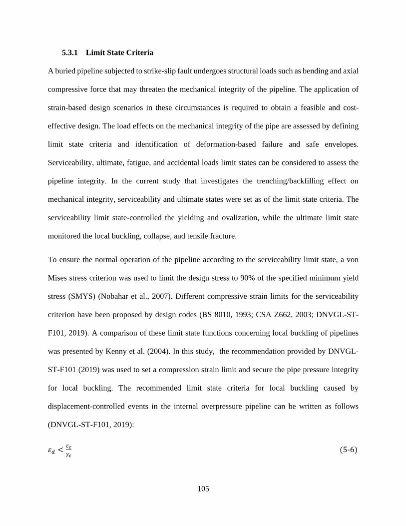
105
5.3.1 Limit State Criteria
A buried pipeline subjected to strike-slip fault undergoes structural loads such as bending and axial
compressive force that may threaten the mechanical integrity of the pipeline. The application of
strain-based design scenarios in these circumstances is required to obtain a feasible and cost-
effective design. The load effects on the mechanical integrity of the pipe are assessed by defining
limit state criteria and identification of deformation-based failure and safe envelopes.
Serviceability, ultimate, fatigue, and accidental loads limit states can be considered to assess the
pipeline integrity. In the current study that investigates the trenching/backfilling effect on
mechanical integrity, serviceability and ultimate states were set as of the limit state criteria. The
serviceability limit state-controlled the yielding and ovalization, while the ultimate limit state
monitored the local buckling, collapse, and tensile fracture.
To ensure the normal operation of the pipeline according to the serviceability limit state, a von
Mises stress criterion was used to limit the design stress to 90% of the specified minimum yield
stress (SMYS) (Nobahar et al., 2007). Different compressive strain limits for the serviceability
criterion have been proposed by design codes (BS 8010, 1993; CSA Z662, 2003; DNVGL-ST-
F101, 2019). A comparison of these limit state functions concerning local buckling of pipelines
was presented by Kenny et al. (2004). In this study, the recommendation provided by DNVGL-
ST-F101 (2019) was used to set a compression strain limit and secure the pipe pressure integrity
for local buckling. The recommended limit state criteria for local buckling caused by
displacement-controlled events in the internal overpressure pipeline can be written as follows
(DNVGL-ST-F101, 2019):
휀𝑑 <𝜀𝑐
𝛾𝜀 (5-6)
106
where 휀𝑑 is design compression strain, 𝛾𝜀 is resistance strain factor equals to 2.6 (Normal safety
class) and 휀𝑐 is compression strain.
휀𝑐 = 0.78 (𝑡
𝐷− 0.01) (1 + 5
𝜎ℎ
𝑓𝑦)
𝛼𝑔𝑤
𝛼ℎ1.5 (5-7)
where 𝑡, 𝐷, 𝜎ℎ, 𝑓𝑦, 𝛼𝑔𝑤, and 𝛼ℎ are the wall thickness; diameter; hoop stress; steel yield stress; girth
weld factor, min (1, 1.2 − 0.01(𝐷 𝑡⁄ )); and strain hardening parameter, respectively. The
compression strain limit has different uncertainties, which will be further discussed in the pipeline
probabilistic fragility section.
5.3.2 Probabilistic Characterization of Seismic Hazard
Using seismic hazard curves, the fault induced ground displacement is usually defined as a
function of the related frequency of occurrence. However, to overcome the shortage of seismic
hazard fault data, the equation proposed by Wells and Coppersmith (1994) was used to determine
the fault displacement that is varied between 0.05 to 8 m for strike-slip faults:
log 𝛿𝑓𝑠 = −6.32 + 0.9𝑀 (5-8)
where 𝛿𝑓𝑠, 𝑀 are average fault displacement and the moment magnitude of the earthquake. The
fault displacements of 1𝐷, 2𝐷, 4𝐷, and 6𝐷 (𝐷 is the diameter of the buried pipe) were selected to
cover the possible fault displacement in the proposed range.
5.3.3 Probabilistic Fragility of the Pipeline
The uncertainties of the pipeline resistance are usually characterized by the fragility curves in the
form of cumulative probabilistic distributions. Other practical methods could be employed to
create fragility curves in case of a lack of experimental or field data. The first solution is to use a

107
two-parameter lognormal distribution for the resistance, where the distribution can be defined by
mean and coefficient of variation. Mohr et al. (2004) performed a strain-based design review using
a complete data set for buckling strain on the pipeline. The results revealed that equation 5-7 almost
indicates the average of the data but creating a probability distribution of compressive strain
capacity for different 𝐷 𝑡⁄ ratio and internal pressure ranges require more available experimental
data. Some of the factors causing uncertainty in the experimental data are: the different test
conditions and experimental methods; different curvature and strain measurement on global and
local scale; and axial load application to refute end cap effects caused by internal pressure during
displacement controlled procedures (Nobahar et al., 2007). The second method is representing the
resistance by a simplified deterministic approach, such as using a factored resistance. Some of the
basis for developing equation 5-7 was reviewed by Vitali et al. (1999) using finite element
assessment, and the results were compared with other available formulations and data. The study
showed that the fitted equation has an error of mean and coefficient of variation of about 0.9 and
20%, respectively. This error only involves uncertainty related to the regression equation and does
not incorporate other sources of ambiguities. Becker (1996) performed a series of calculations and
indicated that by using a resistance strain factor (𝛾𝜀) equal to 2.6 (DNVGL-ST-F101, 2019), the
coefficient of variation expected to be 35%.
Based on these investigations, there are two possible approaches to characterize the strain limits:
i)using a logarithmic distribution with mean value defined by equation 5-7 and coefficient of
variation of 35%, ii)using factored compression strain limit defined by equation 5-6. Table 5-2
represents the key parameters of both methods.

108
Table 5-2. Strain limits characterization
Logarithmic distribution of strain limit Factored compression strain limit
D/t Mean (%) COV (%) 휀𝑐 𝛾𝜀⁄ (%)
48 3.12 35 1.20
35 5.07 35 1.95
24 7.37 35 2.83
In the current study, the factored compression strain limit with the parameter values given in Table
5-2 was utilized to characterize the strain limits.
5.3.4 Probabilistic Characterization of Soil and Trench
The uncertain parameters related to native, and backfill soil along with the trench geometry was
characterized by undrained shear strength of backfill (𝐶𝑢𝑏), undrained shear strength of native
(𝐶𝑢𝑛), soil density (𝛾), trench width (w), and trench depth (d) to construct the database.
The uncertainties regarding systematic test variations and spatial alteration of soil properties were
incorporated by using the lognormal distribution for defining undrained shear strength of backfill
(𝐶𝑢𝑏), undrained shear strength of native (𝐶𝑢𝑛), and soil density (𝛾). The mean and coefficient of
variation were respectively set to 3.06 kPa (μCub), 2.541 kPa (δCub
) for undrained shear strength
of backfill (𝐶𝑢𝑏); 31.72 kPa (μCun) and 0.98 kPa (δCun
) for undrained shear strength of native
(𝐶𝑢𝑛); and 17.5 𝑘𝑁 𝑚3⁄ (μγ) and 0.09 𝑘𝑁 𝑚3⁄ (δγ) for soil density (𝛾) (Ching and Phoon, 2012).
The variation of trench geometry (trench width and depth) were addressed by defining distinct
quantities based on the study conducted by Paulin (1998). For studying trench geometry, two
groups of analyses were conducted with constant trench depth (varying trench width) and constant
trench width (varying trench depth). The trench dimensions for both groups of studies are
summarized in Table 5-3.
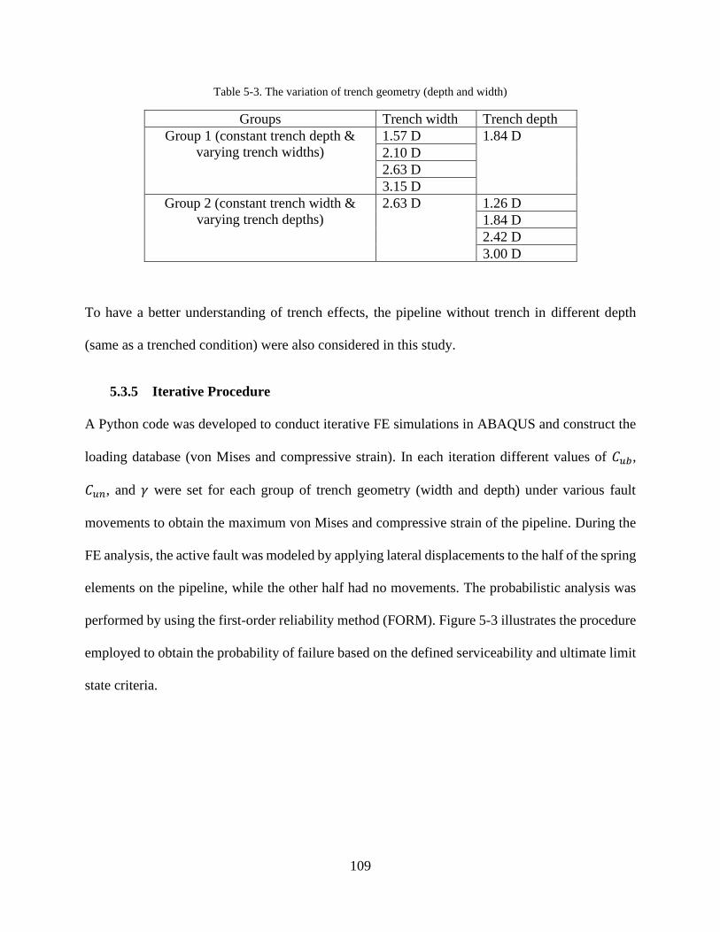
109
Table 5-3. The variation of trench geometry (depth and width)
Groups Trench width Trench depth
Group 1 (constant trench depth &
varying trench widths)
1.57 D 1.84 D
2.10 D
2.63 D
3.15 D
Group 2 (constant trench width &
varying trench depths)
2.63 D 1.26 D
1.84 D
2.42 D
3.00 D
To have a better understanding of trench effects, the pipeline without trench in different depth
(same as a trenched condition) were also considered in this study.
5.3.5 Iterative Procedure
A Python code was developed to conduct iterative FE simulations in ABAQUS and construct the
loading database (von Mises and compressive strain). In each iteration different values of 𝐶𝑢𝑏,
𝐶𝑢𝑛, and 𝛾 were set for each group of trench geometry (width and depth) under various fault
movements to obtain the maximum von Mises and compressive strain of the pipeline. During the
FE analysis, the active fault was modeled by applying lateral displacements to the half of the spring
elements on the pipeline, while the other half had no movements. The probabilistic analysis was
performed by using the first-order reliability method (FORM). Figure 5-3 illustrates the procedure
employed to obtain the probability of failure based on the defined serviceability and ultimate limit
state criteria.
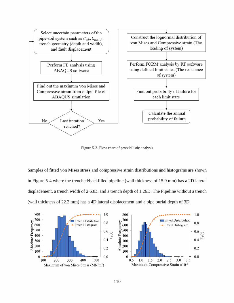
110
Figure 5-3. Flow chart of probabilistic analysis
Samples of fitted von Mises stress and compressive strain distributions and histograms are shown
in Figure 5-4 where the trenched/backfilled pipeline (wall thickness of 15.9 mm) has a 2D lateral
displacement, a trench width of 2.63D, and a trench depth of 1.26D. The Pipeline without a trench
(wall thickness of 22.2 mm) has a 4D lateral displacement and a pipe burial depth of 3D.
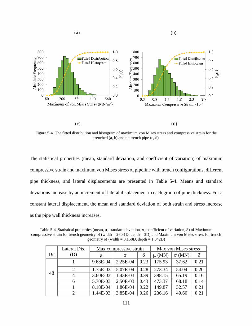
111
(a) (b)
(c) (d)
Figure 5-4. The fitted distribution and histogram of maximum von Mises stress and compressive strain for the
trenched (a, b) and no trench pipe (c, d)
The statistical properties (mean, standard deviation, and coefficient of variation) of maximum
compressive strain and maximum von Mises stress of pipeline with trench configurations, different
pipe thickness, and lateral displacements are presented in Table 5-4. Means and standard
deviations increase by an increment of lateral displacement in each group of pipe thickness. For a
constant lateral displacement, the mean and standard deviation of both strain and stress increase
as the pipe wall thickness increases.
Table 5-4. Statistical properties (mean, ; standard deviation, ; coefficient of variation, ) of Maximum
compressive strain for trench geometry of (width = 2.631D, depth = 3D) and Maximum von Mises stress for trench
geometry of (width = 3.158D, depth = 1.842D)
D/t
Lateral Dis.
(D)
Max compressive strain Max von Mises stress
(MN) (MN)
48
1 9.68E-04 2.25E-04 0.23 175.93 37.62 0.21
2 1.75E-03 5.07E-04 0.28 273.34 54.04 0.20
4 3.60E-03 1.43E-03 0.39 398.15 65.19 0.16
6 5.70E-03 2.50E-03 0.43 473.37 68.18 0.14
1 8.18E-04 1.86E-04 0.22 149.87 32.57 0.21
2 1.44E-03 3.85E-04 0.26 236.16 49.60 0.21
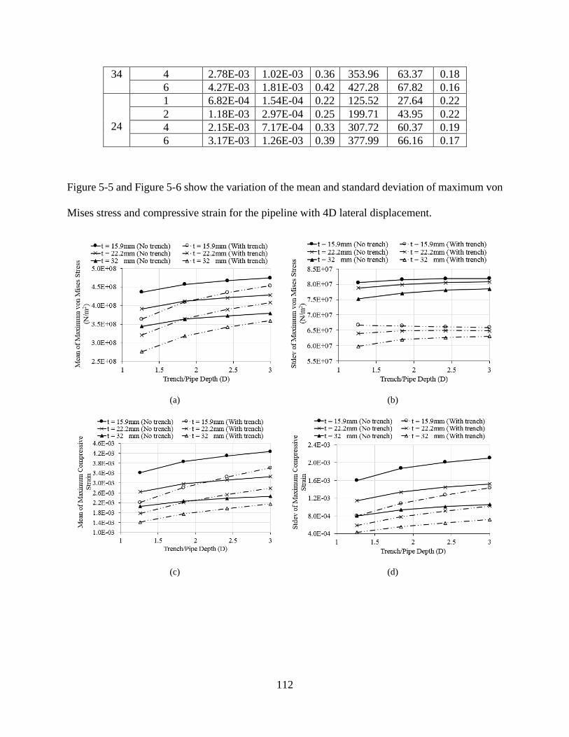
112
34 4 2.78E-03 1.02E-03 0.36 353.96 63.37 0.18
6 4.27E-03 1.81E-03 0.42 427.28 67.82 0.16
24
1 6.82E-04 1.54E-04 0.22 125.52 27.64 0.22
2 1.18E-03 2.97E-04 0.25 199.71 43.95 0.22
4 2.15E-03 7.17E-04 0.33 307.72 60.37 0.19
6 3.17E-03 1.26E-03 0.39 377.99 66.16 0.17
Figure 5-5 and Figure 5-6 show the variation of the mean and standard deviation of maximum von
Mises stress and compressive strain for the pipeline with 4D lateral displacement.
(a)
(b)
(c)
(d)
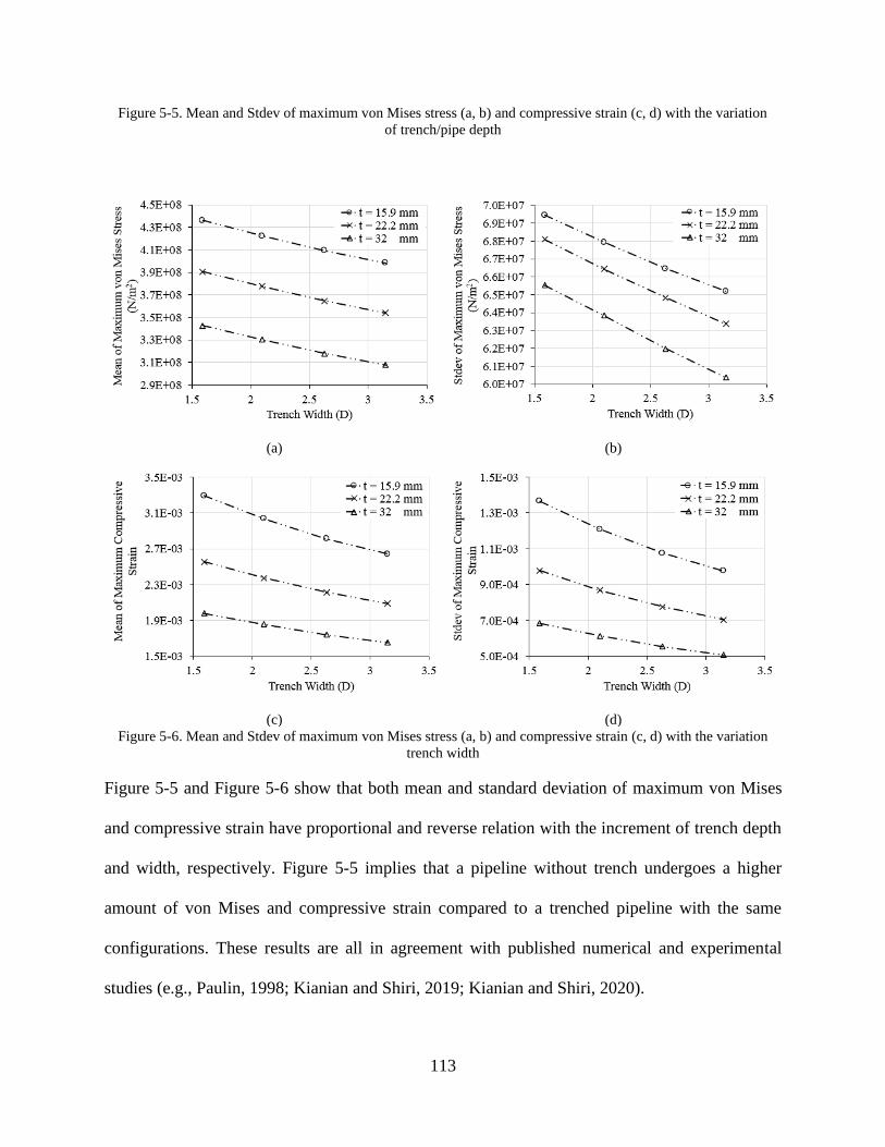
113
Figure 5-5. Mean and Stdev of maximum von Mises stress (a, b) and compressive strain (c, d) with the variation
of trench/pipe depth
(a)
(b)
(c)
(d)
Figure 5-6. Mean and Stdev of maximum von Mises stress (a, b) and compressive strain (c, d) with the variation
trench width
Figure 5-5 and Figure 5-6 show that both mean and standard deviation of maximum von Mises
and compressive strain have proportional and reverse relation with the increment of trench depth
and width, respectively. Figure 5-5 implies that a pipeline without trench undergoes a higher
amount of von Mises and compressive strain compared to a trenched pipeline with the same
configurations. These results are all in agreement with published numerical and experimental
studies (e.g., Paulin, 1998; Kianian and Shiri, 2019; Kianian and Shiri, 2020).
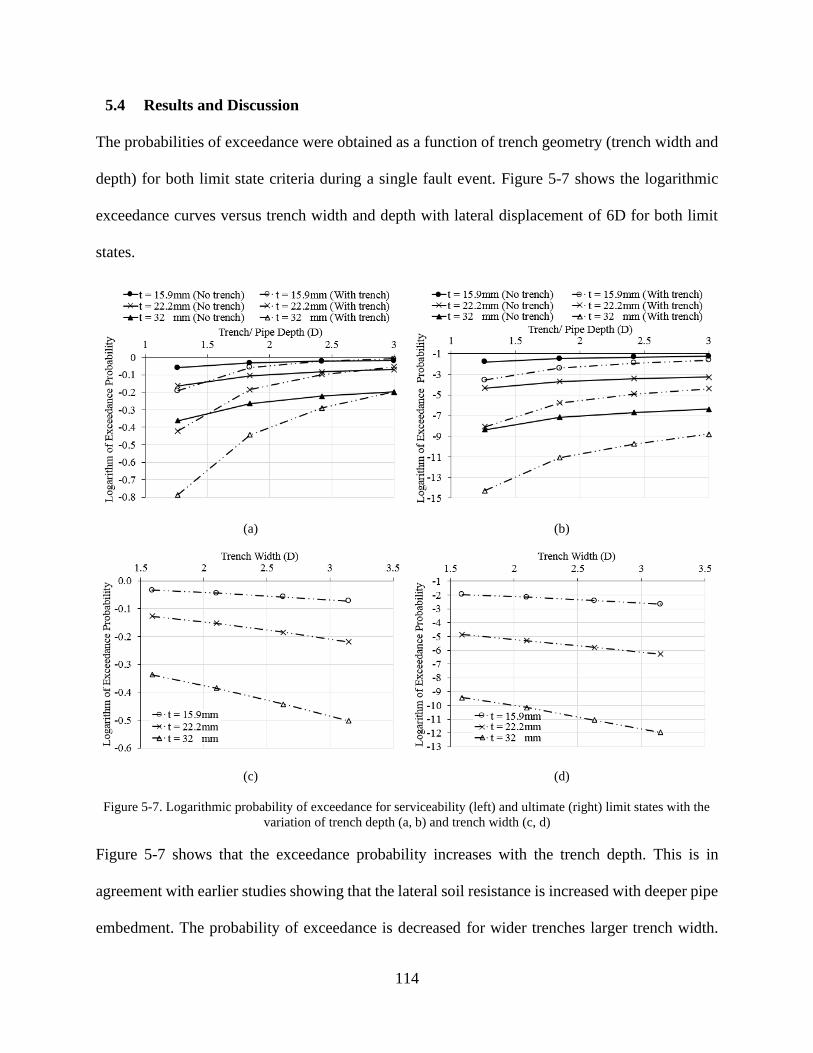
114
5.4 Results and Discussion
The probabilities of exceedance were obtained as a function of trench geometry (trench width and
depth) for both limit state criteria during a single fault event. Figure 5-7 shows the logarithmic
exceedance curves versus trench width and depth with lateral displacement of 6D for both limit
states.
(a)
(b)
(c)
(d)
Figure 5-7. Logarithmic probability of exceedance for serviceability (left) and ultimate (right) limit states with the
variation of trench depth (a, b) and trench width (c, d)
Figure 5-7 shows that the exceedance probability increases with the trench depth. This is in
agreement with earlier studies showing that the lateral soil resistance is increased with deeper pipe
embedment. The probability of exceedance is decreased for wider trenches larger trench width.
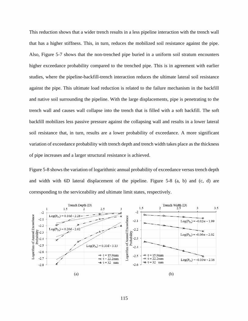
115
This reduction shows that a wider trench results in a less pipeline interaction with the trench wall
that has a higher stiffness. This, in turn, reduces the mobilized soil resistance against the pipe.
Also, Figure 5-7 shows that the non-trenched pipe buried in a uniform soil stratum encounters
higher exceedance probability compared to the trenched pipe. This is in agreement with earlier
studies, where the pipeline-backfill-trench interaction reduces the ultimate lateral soil resistance
against the pipe. This ultimate load reduction is related to the failure mechanism in the backfill
and native soil surrounding the pipeline. With the large displacements, pipe is penetrating to the
trench wall and causes wall collapse into the trench that is filled with a soft backfill. The soft
backfill mobilizes less passive pressure against the collapsing wall and results in a lower lateral
soil resistance that, in turn, results are a lower probability of exceedance. A more significant
variation of exceedance probability with trench depth and trench width takes place as the thickness
of pipe increases and a larger structural resistance is achieved.
Figure 5-8 shows the variation of logarithmic annual probability of exceedance versus trench depth
and width with 6D lateral displacement of the pipeline. Figure 5-8 (a, b) and (c, d) are
corresponding to the serviceability and ultimate limit states, respectively.
(a)
(b)
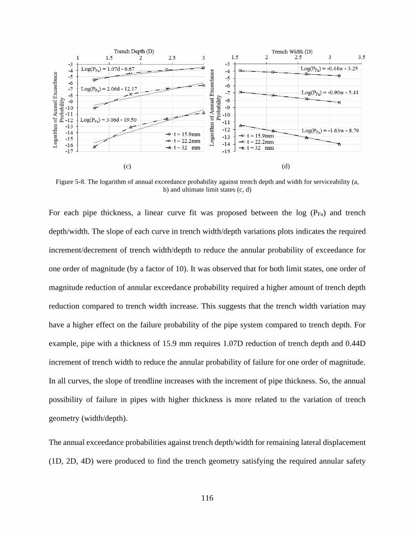
116
(c)
(d)
Figure 5-8. The logarithm of annual exceedance probability against trench depth and width for serviceability (a,
b) and ultimate limit states (c, d)
For each pipe thickness, a linear curve fit was proposed between the log (PFa) and trench
depth/width. The slope of each curve in trench width/depth variations plots indicates the required
increment/decrement of trench width/depth to reduce the annular probability of exceedance for
one order of magnitude (by a factor of 10). It was observed that for both limit states, one order of
magnitude reduction of annular exceedance probability required a higher amount of trench depth
reduction compared to trench width increase. This suggests that the trench width variation may
have a higher effect on the failure probability of the pipe system compared to trench depth. For
example, pipe with a thickness of 15.9 mm requires 1.07D reduction of trench depth and 0.44D
increment of trench width to reduce the annular probability of failure for one order of magnitude.
In all curves, the slope of trendline increases with the increment of pipe thickness. So, the annual
possibility of failure in pipes with higher thickness is more related to the variation of trench
geometry (width/depth).
The annual exceedance probabilities against trench depth/width for remaining lateral displacement
(1D, 2D, 4D) were produced to find the trench geometry satisfying the required annular safety
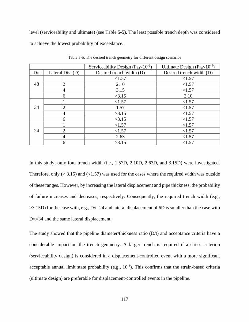
117
level (serviceability and ultimate) (see Table 5-5). The least possible trench depth was considered
to achieve the lowest probability of exceedance.
Table 5-5. The desired trench geometry for different design scenarios
Serviceability Design (PFa<10-3) Ultimate Design (PFa<10-4)
D/t Lateral Dis. (D) Desired trench width (D) Desired trench width (D)
48
1 <1.57 <1.57
2 2.10 <1.57
4 3.15 <1.57
6 >3.15 2.10
34
1 <1.57 <1.57
2 1.57 <1.57
4 >3.15 <1.57
6 >3.15 <1.57
24
1 <1.57 <1.57
2 <1.57 <1.57
4 2.63 <1.57
6 >3.15 <1.57
In this study, only four trench width (i.e., 1.57D, 2.10D, 2.63D, and 3.15D) were investigated.
Therefore, only (> 3.15) and (<1.57) was used for the cases where the required width was outside
of these ranges. However, by increasing the lateral displacement and pipe thickness, the probability
of failure increases and decreases, respectively. Consequently, the required trench width (e.g.,
>3.15D) for the case with, e.g., D/t=24 and lateral displacement of 6D is smaller than the case with
D/t=34 and the same lateral displacement.
The study showed that the pipeline diameter/thickness ratio (D/t) and acceptance criteria have a
considerable impact on the trench geometry. A larger trench is required if a stress criterion
(serviceability design) is considered in a displacement-controlled event with a more significant
acceptable annual limit state probability (e.g., 10-3). This confirms that the strain-based criteria
(ultimate design) are preferable for displacement-controlled events in the pipeline.

118
It is worth mentioning that the construction expenses can be optimized by using the results of the
current study for the appropriate selection of pipeline and trench configurations. As material cost
is often less than trenching cost, the observation in the current study shows that the selection of
robust D/t ratios to mitigate fault movement hazards can result in a cost-effective design using
practical trench geometries. Although, there are other engineering and economic criteria like
material selection, welding, seabed bathymetry, etc. that should be accounted for the design
optimization.
5.5 Conclusions and Recommendations
The probabilistic analysis of buried pipelines under seismic fault hazards was investigated using
the FORM method. A finite element beam-spring model was developed to simulate the pipeline
response to strike faults events. Nonlinear hyperbolic springs were used to model the
trenching/backfilling effects in the lateral pipe-soil interaction. Two limit states based on von
Mises stress and compressive strain of pipeline were employed to differentiate the failure and safe
regions. A phyton code was developed to perform iterative probabilistic analysis with the variation
of native and backfill soil properties, pipe specifications (D/t), and trench geometry under the
different magnitude of lateral fault displacements. The annual probabilities of failure pipeline were
calculated using the Poisson model. The key findings are summarized below:
• Deeper pipe embedment in narrow trenches results in a higher ultimate soil resistance and
a higher annual probability of failure, where the trench width showed a greater impact.
• Pipe diameter to wall thickness ratio (D/t) and the limit state criteria have the most
significant influence on the desired trench geometry.

119
• The proposed probabilistic approach could be used in real pipeline design projects in
seismic regions to optimize pipe specification and trench geometry to have safe and cost-
effective construction.
For a practical application, the methodology developed in the current study can be improved by
deterministic selection of seismic occurrence frequency and fault displacement, incorporation of
the axial and vertical effects of trenching/backfilling in the finite elements analysis, using the
factored method for limit state criteria, and examining a wider range of trench configurations.
Acknowledgment
The authors gratefully acknowledge the financial support of this research by Wood PLC via
establishing the Wood Group Chair in Arctic and harsh environment engineering at Memorial
University, the NL Tourism, Culture, Industry and Innovation (TCII) via CRD collaborative
funding program, the Natural Sciences and Engineering Research Council of Canada (NSERC)
via Engage funding program, the in-kind technical supports and advice of TechnipFMC, NL,
Canada, the Memorial University of Newfoundland through VP start-up fund, and the school of
graduate studies (SGS) baseline fund.
120
References
ALA, 2005. Guidelines for the design of buried steel pipe. Am. Socoiety Civ. Eng. 2001, 29-32,68-
72.
API, A.P.I., 2018. API 5L Specification for line pipe. Api Spec 5L Forty Four, 1–40.
https://doi.org/10.1520/G0154-12A
ASCE Committee, 2014. Soil Parameters for Assessing Axial and Transverse Behavior of
Restrained Pipelines-Part 2: Transverse Behavior. Pipelines 2014: From Underground to
Forefront of Innovation and Sustainability.
Becker, D.E., 1996. Eighteenth Canadian Geotechnical Colloquium: Limit States Design For
Foundations. Part II. Development for the National Building Code of Canada. Can. Geotech.
J. 33, 984–1007.
BS 8010, 1993. Code of Practice for Pipelines Part 3. Pipeline Subsea: Design, Construction and
Installation. Br. Stand. 8010.
C-Core, 2005. Extended model for pipe soil interaction.
C-Core, 2004. Extended model for pipe soil interaction.
C-CORE, 2003. Extended model for pipe soil interaction.
Cheng, Y., Akkar, S., 2017. Measuring bias in structural response caused by ground motion
scaling. Earthq. Eng. Struct. Dyn. 605–620. https://doi.org/10.1002/eqe
Ching, J., Phoon, K.K., 2012. Modeling parameters of structured clays as a multivariate normal
distribution. Can. Geotech. J. 49, 522–545. https://doi.org/10.1139/T2012-015
CSA Z662, 2003. Oil and Gas Pipeline Systems. Can. Stand. Assoc. 2003.
121
Das, B.M., Seeley, G.R., 1975. Pullout resistance of vertical anchors. Geotech. Eng. Div. Soc. Civ.
Eng. 87–91.
DNVGL-RP-F114, 2017. DNVGL RP F114 Rules for pipe-soil interaction for submarine
pipelines. Dnvgl Rp F114 97.
DNVGL-ST-F101, 2019. Submarine Pipeline Systems. Offshore standartd.
Hansen, J.B., 1948. The Stabilizing Effect of Piles in Clay., in: CN Post No. 3, Christiani and
Nielson, Copenhagen, Denmark, November. pp. 14–15.
Hansen, J.B., Christensen, N.H., 1961. The ultimate resistance of rigid piles against transversal
forces. Geoteknisk Institut, Copenhagen 1961.
Karamitros, D.K., Bouckovalas, G.D., Kouretzis, G.P., 2007. Stress analysis of buried steel
pipelines at strike-slip fault crossings. Soil Dyn. Earthq. Eng. 27, 200–211.
https://doi.org/10.1016/j.soildyn.2006.08.001
Kenny, S., Bruce, J., King, T., McKenna, R., Nobahar, A., Phillips, R., 2004. Probabilistic design
methodology to mitigate ice gouge hazards for offshore pipelines, in: International Pipeline
Conference.
Kianian, M., Esmaeilzadeh, M., Shiri, H., 2018. Lateral response of trenched pipelines to large
deformations in clay. Proc. Annu. Offshore Technol. Conf. 5, 3487–3504.
https://doi.org/10.4043/28842-ms
Kianian, M., Shiri, H., 2020. The effect of backfilling stiffness on lateral response of the shallowly
trenched-backfilled pipelines in clay. Mar. Georesources Geotechnol. 0, 1–13.
https://doi.org/10.1080/1064119X.2020.1736699
122
Kianian, M., Shiri, H., 2019. The influence of pipeline–trenchbed interaction intensity on lateral
soil resistance and failure mechanisms. Int. J. Geotech. Eng.
https://doi.org/10.1080/19386362.2019.1709948
Kostyukov, V.D., 1963. DISTRIBUTION OF THE DENSITY OF SAND IN THE SLIDING
WEDGE IN FRONT OF ANCHOR PLATES. Soil Mech. Found. Eng. 12–13.
Mahsuli, M., Haukaas, T., 2013. Computer program for multimodel reliability and optimization
analysis. J. Comput. Civ. Eng. 27, 87–98. https://doi.org/10.1061/(ASCE)CP.1943-
5487.0000204
Merifield, R.S., Sloan, S.W., Yu, H.S., 2001. Stability of plate anchors in undrained clay.
Géotechnique 51, 141–153.
Mohr, B., Gordon, R., Smith, R., 2004. Strain Based Design Guidelines for Pipelines, in: Pipeline
Technology Conference. pp. 291 – 311.
Neely, W.J., Stewart, J.G., Graham, J., 1973. Failure loads of vertical anchor plates in sand. Soil
Mech. Found. Div. Am. Soc. Civ. Eng. 669–685.
Nobahar, A., Kenny, S., King, T., McKenna, R., Phillips, R., 2007. Analysis and design of buried
pipelines for ice gouging hazard: A probabilistic approach. J. Offshore Mech. Arct. Eng. 129,
219–228. https://doi.org/10.1115/1.2426989
Ovesen, N.K., 1964. Anchor slabs, calculation methods and model tests, in: Danish Geotech. Inst.,
Copenhagen, Denmark.
Ovesen, N.K., Stroman, H., 1972. Design methods for vertical anchor plates in sand, in:
Proceedings of Specialty Conference on Performance of Earth at Earth Supported Structures.
123
New York: American Society of Civil Engineers, pp. 1481–1500.
Paulin, M., 1998. An investigation into pipelines subjected to lateral soil loading.” Ph.D. thesis,
Ph.D. thesis, Memorial University of Newfoundland, St. John’s, Canada.
Phillips, R., Nobahar, A., Zhou, J., 2004. TRENCH EFFECTS ON PIPE-SOIL INTERACTION,
in: International Pipeline Conference.
PRCI, 2009. Guidelines for Constructing Natural Gas and Liquid Hydrocarbon Pipelines Through
Areas Prone to Landslide and Subsidence Hazards. Des. Mater. Constr. Comm. Pipeline Res.
Counc. Int. Inc.
Rowe, R.K., Davis, E.H., 1982. The behaviour of anchor plates in clay. Géotechnique 32, 25–41.
Smith, J.E., 1962. Deadman anchorages is sand. Technical report R199.
Takada, S., Hassani, N., Fukuda, K., 2001. A new proposal for simplified design of buried steel
pipes crossing active faults. Earthq. Eng. Struct. Dyn. 30, 1243–1257.
https://doi.org/10.1002/eqe.62
Vitali, L., Bruschi, R., Mork, K.J., Levold, E., Verley, R., 1999. Hotpipe Project: Capacity of Pipes
Subject to Internal Pressure, Axial Force and Bending Moment, in: Proceedings of the Ninth
International Offshore and Polar Engineering Conference. pp. 22–33.
Walker, A.C., Williams, K.A.J., 1995. Strain Based Design of Pipelines, in: 14th OMAE. pp. 345–
350.
Wantland, G.M., O’Neill, M.W., Reese, L.C., Kalajian, E.H., 1979. Lateral stability of pipelines
in clay, in: Proceedings of the Annual Offshore Technology Conference. pp. 1025–1034.
Wells, D.L., Coppersmith, K.J., 1994. New empirical relationships among magnitude, rupture

124
length, rupture width, rupture area, and surface displacement. Bull. - Seismol. Soc. Am. 84,
974–1002.
Winkler, E., 1867. Die leher von der elastizitat und festigkeit. Dominicus, Prague 1867.

125
Chapter 6. Summary, Conclusions and recommendations
6.1 Drag Embedment Anchor-Seabed Interaction
The reliability of drag embedment anchors in the sand and layered soil (clay over sand) were
investigated for catenary mooring systems and compared with earlier studies in clay. The
reliability analyses were carried out by adopting the first order reliability method (FORM) using
two popular Stevpris anchor families, MK5 and MK6. The limit state function was established at
the mudline, while the chain-soil interaction effects were accounted for in the calculation of
ultimate holding capacities. Fully coupled time-domain analyses were conducted to simulate the
station keeping of a generic semisubmersible platform to obtain the dynamic mooring line
tensions. The generic semisubmersible platform located in the Caspian Sea for sand seabed and
Flemish Pass Basin, Newfoundland, for clay over sandy soil were selected. The response surface
method was adopted for probabilistic modeling of the line tensions at the mudline. Two Excel
spreadsheets containing VBA macros were developed and validated to predict the ultimate anchor
capacity and the anchor trajectory down the seabed by incorporation of a popular limit state model
in the sand and layered (clay over sand) seabed. The variation of annual reliability indices and the
logarithm of the failure probabilities versus the fluke length and the anchor weight were obtained
and compared with existing studies in each study. The important conclusions are summarized
below:
• The geometrical configuration of the anchors, particularly the fluke length, are the most
influential parameters in determining the reliability indices. The anchor weight has a
beneficial contribution to achieving a higher level of reliability but to a less extent. A well-
designed anchor geometry can significantly dominate the weight effect. For instance, some

126
lighter MK6 anchors result in a higher reliability index compared to heavier MK5 models
due to their superior geometrical design.
• The costly in-field testing procedure recommended by design codes for estimation of the
anchor capacities are unique for all of the anchor groups, seabed soil types, environmental
loads, and operation conditions. This approach ignores the reliability effects affected by a
wide range of inherent uncertainties and limits the cost-effectiveness of the proposed
solutions. Further reliability-based refinement of the proposed procedures can have
significant cost effects on offshore projects.
• A target reliability index for a given anchor group in clay can be achieved by a heavier
anchor compared to the sand. It is challenging to determine a corresponding set of soil
parameters in clay and sand to result in an identical reliability index. However, further
studies in this area can be beneficial in proposing a more cost-effective infield testing
procedure.
• The seabed soil stratum and its configuration (individual layer thickness) have a significant
influence on reliability indices. Overall, the probability of failure is higher for the layered
clay over sand stratum compared with homogeneous clay and sand layers. This suggests
that the recommended practices that are currently considering only similar soil should be
re-assessed and possibly improved for complex, layered seabed soil strata.
• The geometrical anchor configuration, particularly the fluke length, was found to have a
significant effect on holding capacity and consequently the reliability indices. The anchor
weight showed a positive influence on reliability results, but less effective than the fluke
length. The geometrical improvement of the anchors can effectively improve their
reliability. In addition, the current design practice is identical for all of the different anchor
127
families. This approach does not account for the significant influence of anchor geometry
and the uncertainties associated with different anchor families, environmental, and
operational loads. The reliability-based refinement of the design procedure can
considerably improve the reliability and cost-effectiveness of anchor design.
• The configuration of layered soil strata, particularly the depth and thickness of layers,
showed a significant effect on the ultimate holding capacity and reliability indices. Thicker
clay layers resulted in higher reliability indices. Different range of layer thickness still
needs to be investigated to generalize the obtained results.
6.2 Lateral Pipeline-Backfill-Trench Interaction
The FORM method was utilized to perform the probabilistic analysis of buried pipelines under
seismic fault movements with consideration of trench effects in clay. The mechanical response of
the pipe to fault movements was captured by a three-dimensional FE element model using the
nonlinear beam-spring method integrated with trench effects. Two limit states based on von Mises
stress and compressive strain were anticipated. The iterative calculations were performed by
variation of native soil, backfill, pipe specifications (D/t), trench geometry under the different
magnitude of lateral fault displacement events using developed python code. The Poisson model
was employed to calculate the annual probability of failure. The key findings are summarized
below:
• Deeper pipe embedment in narrow trenches results in a higher ultimate soil resistance and
a higher annual probability of failure, where the trench width showed a greater impact.
• Pipe diameter to wall thickness ratio (D/t) and the limit state criteria have the most
significant influence on the desired trench geometry.
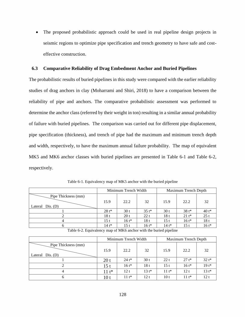
128
• The proposed probabilistic approach could be used in real pipeline design projects in
seismic regions to optimize pipe specification and trench geometry to have safe and cost-
effective construction.
6.3 Comparative Reliability of Drag Embedment Anchor and Buried Pipelines
The probabilistic results of buried pipelines in this study were compared with the earlier reliability
studies of drag anchors in clay (Moharrami and Shiri, 2018) to have a comparison between the
reliability of pipe and anchors. The comparative probabilistic assessment was performed to
determine the anchor class (referred by their weight in ton) resulting in a similar annual probability
of failure with buried pipelines. The comparison was carried out for different pipe displacement,
pipe specification (thickness), and trench of pipe had the maximum and minimum trench depth
and width, respectively, to have the maximum annual failure probability. The map of equivalent
MK5 and MK6 anchor classes with buried pipelines are presented in Table 6-1 and Table 6-2,
respectively.
Table 6-1. Equivalency map of MK5 anchor with the buried pipeline
Minimum Trench Width Maximum Trench Depth
Pipe Thickness (mm) Lateral Dis. (D)
15.9
22.2
32
15.9
22.2
32
1 28 t* 30 t 35 t* 30 t 38 t* 40 t* 2 18 t 20 t 22 t 18 t 21 t* 25 t 4 15 t 16 t* 18 t 15 t 16 t* 18 t 6 14 t* 15 t 16 t* 14 t* 15 t 16 t*
Table 6-2. Equivalency map of MK6 anchor with the buried pipeline
Minimum Trench Width Maximum Trench Depth
Pipe Thickness (mm) Lateral Dis. (D)
15.9
22.2
32
15.9
22.2
32
1 20 t 24 t* 30 t 22 t 27 t* 32 t*
2 15 t 16 t* 18 t 15 t 16 t* 19 t*
4 11 t* 12 t 13 t* 11 t* 12 t 13 t*
6 10 t 11 t* 12 t 10 t 11 t* 12 t
129
It should be mentioned that in both Table 6-1 and Table 6-2, anchors were identified by their
weights in the unit of ton(t), and the cells with star sign(*) correspond to anchor weight which are
not offered in the Veryhof anchor manual. Overall, the study showed that the conventional
equations commonly used between the anchors and pipelines could be reasonably used for the
reliability of anchors and pipelines in uniform soils. However, involving more realistic scenarios
with non-homogenous and layered soils significantly affects the failure mechanisms and ultimate
soil resistance, consequently. Therefore, further improved models to account for complex soil
strata is recommended for future studies.
6.4 Recommendations for Future Studies
Most essential features that could be recommended for consideration in the future studies are as
follows:
a) Suggestion for Drag Embedment Study
• The existing anchor solutions are developed based on simplified anchor geometries. The
idealization of anchor geometry may have a significant impact on reliability results.
However, the impact is not significant in comparative studies. Further investigations are
required to determine the best practice for the idealization of anchor geometry in analytical
solutions.
• The reliability models for assessing the anchor capacities can be significantly improved by
having access to the in-field test databases and corresponding seabed soil properties, and
the statistics of failures.
• Further studies could find a corresponding relationship between soil parameters in sand
and clay to have a matching reliability index.
130
• Developing more robust anchor-seabed interaction models to account for the complex
layered soil strata would significantly improve the results of reliability analysis.
b) Recommendation for Buried Subsea Pipelines
• Developing new models for incorporation of trenching/backfilling effect in pipe-soil
interaction analysis.
• Employing deterministic seismic occurrence frequency and fault displacement. Selecting
the probabilistic occurrence frequency would be a better option.
• Incorporation of the trenching/backfilling impacts on pipeline response in axial and vertical
directions.
• Using the factored method for limit state criteria.
• Employing more trench geometries for better quantification of optimum trench geometry.
131
References
ALA, 2005. Guidelines for the design of buried steel pipe. Am. Socoiety Civ. Eng. 2001, 29-32,68-
72.
Almahakeri, M., Fam, A., Moore, I.D., 2013. Longitudinal bending and failure of GFRP pipes
buried in dense sand under relative ground movement. J. Compos. Constr. 17, 702–710.
https://doi.org/10.1061/(ASCE)CC.1943-5614.0000340
API RP 2SK, 2008. Design and Analysis of Stationkeeping Systems for Floating Structures.
ASCE, 2001. Guidelines for the seismic design of oil and gas pipeline systems. ” American Society
of Civil Engineers, Committee on gas and liquid fuel life lines, Technical Council on Life
line Earthquake Engineering, ASCE, New York. 1984.
Audibert, J.M.E., Lai, N.., Bea, R.G., 1979. Design of Pipelines- Sea Bottom Loads and Restraints,
Pipelines in Adverse Environments: A State of the Art. ASCE 1, 187–203.
Bhushan, K., Haley, S.C., Fong, P.T., 1979. Lateral Load Tests on Drilled Piers in Stiff Clays. J.
Geotech. Eng. Div. ASCE 105, 969–985.
Bjerager, R., 1991. Methods for structural reliability computation. In: Casciati F, editor. Reliability
problems: general principles and applications in mechanics of solid and structures. New York;
Springer Verlag, 1991. p. 89-136.
C-CORE, 2003. Extended model for pipe soil interaction.
Choi, Y.J., 2007. Reliability Assessment of Foundations for Offshore Mooring Systems under
Extreme Environments.
Clukey, E.C., Gilbert, R.B., Andersen, K.H., Dahlberg, R., 2013. Reliability of Suction Caissons
132
for Deep Water Floating Facilities 1991, 456–474.
https://doi.org/10.1061/9780784412763.035
Craig, W.H., 1994. Size effects in anchor performance. Can. Geotech. J. 31, 450–454.
https://doi.org/10.1139/t94-052
Das, B.M., Moreno, R., Dallo, K., 1985. Ultimate pullout capacity of shallow vertical anchors in
clay. Soils Found. 2091.
Das, B.M., Tarquin, A.J., Marino, R., 1987. Model Tests for Pullout Resistance of Vertical
Anchors in Clay. Soils Found. 17, 52–56.
Degenkamp, B.G., Dutta, A., 1989. Soil resistances to embedded anchor chain in soft clay 115,
1420–1438.
Dickin, E.A., 1994. Uplift resistance of buried pipelines in sand 41–48.
Ditlevsen, O., 1981. Principle of Normal Tail Approximation. J. Eng. Mech. Div. 107, 1191–1207.
DNV, 2007. Global Buckling of Submarine Pipelines–Structural Design to High
Temperature/High Pressure. Dnv-Rp-F110.
DNV, 2000. Design and installation of fluke anchors in clay. Recommended Practice RP-301. Det
Nor. Verit. 28.
Dunnavant, T.W., Kwan, C.-T.T., 1993. Centrifuge Modelling And Parametric Analyses Of Drag
Anchor Behavior, in: Offshore Technology Conference. https://doi.org/10.4043/7202-ms
EGIG, 2005. Gas Pipeline Incidents, European Gas Pipeline Incident Data Group, Groningen, the
Netherlands 6th EGIG Report 1970-2004, No. EGIG 05-R-0002.
133
Felix, S., Wong, M., 1985. SLOPE RELIABILITY AND RESPONSE SURFACE METHOD.
Geotech. Eng. 111, 32–53.
Fulton, T.M., Stewart, W.P., 1994. Vertical loads on drag embedment anchors. Proc. Annu.
Offshore Technol. Conf. 1994–May, 233–241. https://doi.org/10.4043/7491-ms
Guo, P.J., Stolle, D.F.E., 2005. Lateral Pipe–Soil Interaction in Sand with Reference to Scale
Effect. J. Geotech. Geoenvironmental Eng. 131, 987–1003.
https://doi.org/10.1061/(ASCE)1090-0241(2005)131
Hansen, J.B., Christensen, N.H., 1961. The ultimate resistance of rigid piles against transversal
forces. Geoteknisk Institut, Copenhagen 1961.
Hasofer, A.M., Lind, N.C., 1974. Exact and Invariant Second-Moment Code Format. J. Eng.
Mech. Div. ASCE 100, 111–121.
Hohenbichler, M., Rackwitz, R., 1981. Non-Normal Dependant Vectors in Structural Safety. J.
Eng. Mech. Div. 107, 1227–1238.
Jung, J.K., O’Rourke, T.D., Olson, N.A., 2013. Lateral soil-pipe interaction in dry and partially
saturated sand. J. Geotech. Geoenvironmental Eng. 139, 2028–2036.
https://doi.org/10.1061/(ASCE)GT.1943-5606.0000960
Kianian, M., Shiri, H., 2019. The influence of pipeline–trenchbed interaction intensity on lateral
soil resistance and failure mechanisms. Int. J. Geotech. Eng.
https://doi.org/10.1080/19386362.2019.1709948
Klar, A., Randolph, M.F., 2008. Upper-bound and load–displacement solutions for laterally loaded
piles in clays based on energy minimisation. Géotechnique 58, 815–820.

134
https://doi.org/10.1680/geot.2007.00197
LeLievre, B., Tabatabaee, J., 1981. Performance of Marine Anchors With Planar Flukes in Sand.
Can. Geotech. J. 18, 520–534. https://doi.org/10.1139/t81-063
Liu, P.L., Der Kiureghian, A., 1991. Optimization Algorithms for Structural Reliability. Struct.
Saf. 9, 161–177. https://doi.org/10.12681/eadd/1834
Lucia Faravelli, 1990. RESPONSE-SURFACE APPROACH FOR RELIABILITY ANALYSIS
By Lucia Faravelli 1. J. Eng. Mech. 115, 2763–2781.
Luscher, U., Thomas, H.P., Maple, J.A., 1979. Pipe – Soil Interaction. Trans-Alaska Pipeline.”
Pipelines in Adverse Environments: A State of the Art. ASCE 486–502.
Madsen, H., Krenk, S., Lind, N., 1986. Methods of structural safety. Englewood Cliffs, NJ:
Prentice- Hall, Inc, 1986.
Merifield, R.S., Sloan, S.W., Yu, H.S., 2001. Stability of plate anchors in undrained clay.
Géotechnique 51, 141–153.
Moharrami, M.J., Shiri, H., 2018. Reliability assessment of drag embedment anchors in clay for
catenary mooring systems. Mar. Struct. 58, 342–360.
https://doi.org/10.1016/j.marstruc.2017.12.005
Montes-Iturrizaga, R., Heredia-Zavoni, E., 2016. Reliability analysis of mooring lines using
copulas to model statistical dependence of environmental variables. Appl. Ocean Res. 59,
564–576. https://doi.org/10.1016/j.apor.2016.07.008
NCEL, 1987a. Naval Civil Engineering Laboratory Naval Civil Engineering Laboratory (Port
Hueneme, 1987. Drag embedment anchors for navy moorings (Vol. 83, No. 8).
135
Neubecker, S.R., 1995. The behaviour of drag anchor and chain systems, PhD Thesis, Department
of Civil Engineering, The University of Western Australia.
Neubecker, S.R., Randolph, M.F., 1996a. The performance of drag anchor and chain systems in
cohesive soil. Georesources Geotech. 14, 1–7.
Neubecker, S.R., Randolph, M.F., 1996b. The kinematic behaviour of drag anchors in sand. Can.
Geotech. J. 33, 584–594. https://doi.org/https://doi.org/10.1139/t96-084-306
Neubecker, S.R., Randolph, M.F., 1996c. The static equilibrium of drag anchors in sand. Can.
Geotech. J. 33, 574–583.
Ng, C.F., 1994. Behaviour of Buried Pipelines Subjected to External Loading.
Nobahar, A., Kenny, S., King, T., McKenna, R., Phillips, R., 2007. Analysis and design of buried
pipelines for ice gouging hazard: A probabilistic approach. J. Offshore Mech. Arct. Eng. 129,
219–228. https://doi.org/10.1115/1.2426989
O’Neill, M.P., 2000. The behaviour of drag anchors in layered soils, PhD Thesis, Department of
Civil Engineering, The University of Western Australia.
O’Neill, M.P., Bransby, M.F., Randolph, M.F., 2003. Drag anchor fluke–soil interaction in clays.
Can. Geotech. J. 40, 78–94. https://doi.org/10.1139/t02-096
Paulin, M., 1998. An investigation into pipelines subjected to lateral soil loading.” Ph.D. thesis,
Ph.D. thesis, Memorial University of Newfoundland, St. John’s, Canada.
Phillips, R., Nobahar, A., Zhou, J., 2004. TRENCH EFFECTS ON PIPE-SOIL INTERACTION,
in: International Pipeline Conference.
Poulos, H.G., 1988. Marine Geotechnics. Unwin Hyman, London, 473p.

136
PRCI, 2009. Guidelines for Constructing Natural Gas and Liquid Hydrocarbon Pipelines Through
Areas Prone to Landslide and Subsidence Hazards. Des. Mater. Constr. Comm. Pipeline Res.
Counc. Int. Inc.
Rackwitz, R., 1982. Response surfaces in structural reliability Sonderforschungsbereich 96.
Reese, L.C., Welch, R.C., 1975. Lateral Loading of Deep Foundations in Stiff Clay. J. Geotech.
Eng. 101, 633–649.
Rendón-Conde, C., Heredia-Zavoni, E., 2016. Reliability analysis of suction caissons for moored
structures under parameter uncertainties. Struct. Saf. 60, 102–116.
https://doi.org/10.1016/j.strusafe.2016.02.004
Rowe, R.K., Davis, E.H., 1982. The behaviour of anchor plates in clay. Géotechnique 32, 25–41.
Saurwalt, K.J., 1974. Anchors digging in and holding in a soft planar seabed.
Silva-González, F., Heredia-Zavoni, E., Valle-Molina, C., Sánchez-Moreno, J., Gilbert, R.B.,
2013. Reliabilitystudy of suction caissons for catenary and taut-leg mooring systems. Struct.
Saf. 45, 59–70. https://doi.org/10.1016/j.strusafe.2013.08.011
Stewart, D.., 1992. Lateral loading of piled bridge abutments due to embankment construction. Ph.
D thesis, Univ. of Western Australia.
Stewart Technology Associate, 1995. STA ANCHOR.
Tabatabaee, J., 1980. Theoretical and experimental investigations on marine anchors, PhD Thesis,
Department of Civil Engineering, The University of Waterloo.
0241(1998)124:10(945)
137
Thorne, C.P., 1998. Penetration and load capacity of marine drag anchors in soft clay. J. Geotech.
Geoenvironmental Eng. 124, 945–953. https://doi.org/10.1061/(ASCE)1090-
0241(1998)124:10(945)
Trautmann, C.H., O’Rourke, T.D., 1985. Lateral force-displacement of buried pipe response. J.
Geotech. Eng. 111, 1077–1092. https://doi.org/0733-9410/85/0009- 1077/$01.00
Tschebotarioff, G.P., 1973. Foundations, Retaining and Earth Structures . McGraw-Hill Book
Company. New York .
Valle-molina, C., Heredia-zavoni, E., Silva-gonzález, F.L., 2008. Reliability analyses of suction
caissons for FPSO systems, in: International Conference on Offshore Mechanics and Arctic
Engineering. pp. 1–6.
Vivatrat, V., Valent, P.J., Ponterio, A.A., 1982. The influence of chain friction on anchor pile
design. Proc. Annu. Offshore Technol. Conf. 1982–May, 153–156.
https://doi.org/10.4043/4178-ms
Xie, X., Symans, M.D., O’Rourke, M.J., Abdoun, T.H., O’Rourke, T.D., Palmer, M.C., Stewart,
H.E., 2013. Numerical modeling of buried HDPE pipelines subjected to normal faulting: A
case study. Earthq. Spectra 29, 609–632. https://doi.org/10.1193/1.4000137
Yimsiri, S., Soga, K., Yoshizaki, K., Dasari, G.R., O’Rourke, T.D., 2004. Lateral and Upward
Soil-Pipeline Interactions in Sand for Deep Embedment Conditions. J. Geotech.
Geoenvironmental Eng. 23, 1390–1392. https://doi.org/10.1061/(ASCE)1090-
0241(2004)130
Zhao, Y.G., Ono, T., 1999. A General Procedure for First/Second-Order Reliability Method

138
(FORM/SORM). Struct. Saf. 21, 95–112.