reliable estimation of generalized linear mixed models...
TRANSCRIPT

The Stata Journal (2002)2, Number 1, pp. 1–21
Reliable estimation of generalized linear mixedmodels using adaptive quadrature
Sophia Rabe-HeskethInstitute of PsychiatryKing’s College London
Anders SkrondalNational Institute ofPublic Health, Oslo
Andrew PicklesSchool of Epidemiology and Health Science
The University of Manchester
Abstract. Generalized linear mixed models or multilevel regression models havebecome increasingly popular. Several methods have been proposed for estimatingsuch models. However, to date there is no single method that can be assumedto work well in all circumstances in terms of both parameter recovery and com-putational efficiency. Stata’s xt commands for two-level generalized linear mixedmodels (e.g., xtlogit) employ Gauss–Hermite quadrature to evaluate and maxi-mize the marginal log likelihood. The method generally works very well, and oftenbetter than common contenders such as MQL and PQL, but there are cases wherequadrature performs poorly. Adaptive quadrature has been suggested to overcomethese problems in the two-level case. We have recently implemented a multilevelversion of this method in gllamm, a program that fits a large class of multilevellatent variable models including multilevel generalized linear mixed models. Asfar as we know, this is the first time that adaptive quadrature has been proposedfor multilevel models. We show that adaptive quadrature works well in problemswhere ordinary quadrature fails. Furthermore, even when ordinary quadratureworks, adaptive quadrature is often computationally more efficient since it requiresfewer quadrature points to achieve the same precision.
Keywords: st0005, adaptive quadrature, gllamm, generalized linear mixed models,random-effects models, panel data, numerical integration, adaptive integration,multilevel models, clustered data
1 Introduction
Generalized linear models, see, for example, McCullagh and Nelder (1989), are regres-sion models for different response types. The models are constructed by defining a linearpredictor
ηi = x′iβ
specifying the functional relationship or link between this predictor and the expectationof the response and selecting a distribution for the response given its expectation. Herexi are explanatory variables for unit i with fixed effects β.
Generalized linear mixed models, see, for example, Goldstein (1995) and McCullochand Searle (2001), include both fixed and random effects in the linear predictor. The
c© 2002 Stata Corporation st0005

2 Estimation of generalized linear mixed models
models are used for grouped or clustered data where observations within a cluster can-not be assumed to be mutually independent. Examples are panel data with repeatedobservations on subjects or two-stage surveys where elementary units are nested in pri-mary sampling units; for example, children in schools. In the simplest generalized linearmixed models, the dependence structure of clustered data is modeled by introducing arandom intercept into the linear predictor. The random intercept is shared by all unitsin the same cluster and can be interpreted as cluster level unobserved heterogeneity.Let i index the elementary “level 1” units and j index the clusters or “level 2” units.Conditional on the random intercept, the model is a generalized linear model with linearpredictor
ηij = x′ijβ + u
(2)j (1)
where xij are explanatory variables with fixed coefficients β, and u(2)j is a random
intercept at level 2. The random intercept is assumed to have a normal distributionwith mean 0. Models of this kind can be fitted using Stata’s panel data commands,xtreg, xtlogit, xtpois, xtclog, and so on.
The model can be extended in two ways. First, random coefficients can be included,allowing the effects of covariates to vary between level-2 units. Second, if the data aremultilevel with several levels of clustering (e.g., repeated observations on children inschools), higher level random effects (intercepts and coefficients) can be included in themodel. Omitting subscripts for the units of observation, the most general form of thelinear predictor for the L-level case is
η = x′β +L∑
l=2
z(l)′u(l)
where z(l) are covariates (generally subsets of x) with random effects u(l) at level l. Thefirst element of each z(l) is typically equal to 1 so that the first element of u(l) representsa random intercept. The random effects at level l are assumed to have a multivariatenormal “prior” distribution with
u(l) ∼ N(0,Σl)
and to be independent of the random effects at any of the other levels. These multileveland random-coefficient models are not available among Stata’s xt panel data modelsbut can be fitted using gllamm; see Rabe-Hesketh et al. (2000), Rabe-Hesketh et al.(2001a), and Rabe-Hesketh et al. (2001b), since they are special cases of “generalizedlinear latent and mixed models”.
In Section 2, we discuss estimation of generalized linear mixed models and describein detail the implementation in gllamm of both quadrature and adaptive quadrature; inSection 3, we describe the syntax of gllamm; and in Section 4, we analyze two datasetsthat have previously been analyzed by other methods.

S. Rabe-Hesketh, A. Skrondal, and A. Pickles 3
2 Estimation of generalized linear mixed models
The likelihood of the observed data is a marginal likelihood where the random effectshave been “integrated out”. Unfortunately, this marginal likelihood does not generallyhave a closed-form expression and approximate methods of estimation must be used.The most commonly used methods include marginal quasi-likelihood (MQL), penalizedquasi-likelihood (PQL), Markov Chain Monte Carlo (MCMC), and Gaussian quadrature(GQ). A promising improvement of Gaussian quadrature is adaptive Gaussian quadra-ture (AGQ).
2.1 MQL, PQL, and MCMC
The methods MQL and PQL have been derived in a number of ways; see, for example,McCulloch and Searle (2001). Here we summarize the description in Goldstein (1995).The idea is that linear models can be estimated in a straightforward way by iteratingbetween (1) generalized least squares to estimate the fixed parameters β for a givencovariance matrix of the responses (which depends on the Σl), and (2) estimating theΣl from the residuals y−x′β, an algorithm known as iterative generalized least squares(IGLS). MQL and PQL are based on approximating generalized linear mixed models aslinear mixed models so that the IGLS algorithm can be applied.
In generalized linear mixed models, the expectation of the response is
µ = g−1(x′β +L∑
l=1
z(l)′u(l)) (2)
where g−1(·) is an inverse link function. For given current parameter estimates, thismodel can be approximated as a linear mixed model by expanding the inverse linkfunction as a Taylor series expansion and representing the variability of the response yaround its mean by a heteroskedastic error term with variance function equal to that ofthe chosen distribution family. That is, for dichotomous responses,
y = µ + ε√
π(1 − π)
where var(ε) = 1 and π is the current predicted probability.
In MQL and PQL, (2) is expanded around the “current” linear predictor. A first-order Taylor series expansion is used with respect to the fixed effects and a first- orsecond-order expansion with respect to the random effects. In MQL, the current linearpredictor is obtained by substituting current estimates for the fixed effects and zero forthe random effects. In PQL, the expansion is improved by setting the random effectsequal to their posterior means instead of zero. MQL and PQL are available in MLwiN(see Goldstein et al. 1998) and in HLM (see Bryk et al. 1996).
MCMC is a simulation approach. By assuming an a priori distribution for the modelparameters, samples of parameter values are drawn from their posterior distributionusing simulation. Since the required joint posterior distribution is generally intractable,

4 Estimation of generalized linear mixed models
it is not possible to simulate directly from this distribution. Instead, a Markov chainis used in which subsets of parameters are sequentially sampled from their conditionaldistributions given current values of the other parameters. After a burn-in period, whenthis chain has become stationary, the sampled parameter values follow the requireddistribution. The mean, median, or mode of these sampled parameters are then usedas parameter estimates. The parameter estimates are essentially maximum likelihoodestimates if the prior distributions are vague or diffuse. MCMC is available in MLwiNand in BUGS; see Spiegelhalter et al. (1996).
2.2 Gaussian quadrature
Gaussian quadrature can be used to approximate the marginal likelihood by numericalintegration. Let θ be the vector of all model parameters including the fixed coefficientsβ and the non-duplicated elements of the covariance matrices Σl. Further let y(l) bethe response vector, X(l) the design matrix with rows (x′, z(2)′, . . . , z(L)′) for all unitsin a particular level-l unit and U (l) = (u(l)′, . . . , u(L)′)′. Let the conditional likelihoodcontribution of a level-1 unit given the random effects be denoted f (1)(θ; y(1),X(1)|U (2)).Depending on the chosen family, this could, for instance, be a Poisson or binomialprobability. The conditional likelihood contribution of a level-2 unit given the randomeffects at levels 3 and above is
f (2)(θ; y(2),X(2)|U (3)) =∫
g(2)(u(2))∏
f (1)(θ; y(1),X(1)|U (2))du(2)
where g(l)(u(l)) is the multivariate normal density with mean 0 and covariance matrixΣl and the product is over all level-1 units within the level-2 unit. The conditionallikelihood contribution of an l-level unit is obtained recursively from the conditionallikelihood contributions of the (l − 1)-level units within it.
f (l)(θ; y(l),X(l)|U (l+1)) =∫
g(l)(u(l))∏
f (l−1)(θ; y(l−1),X(l−1)|U (l))du(l) (3)
The total likelihood is
f(θ; y,X) =∏∫
g(L)(u(L))∏
f (L−1)(θ; y(L−1),X(L−1)|u(L))du(L)
where y and X are the vector of responses and design matrix for all units and the firstproduct is over all highest level units.
For given parameter values, the multivariate integral over the Ml random effects vari-ables u(l) at level l is evaluated by integrating over Ml independent standard normallydistributed random effects v(l) with u(l) = Clv
(l), where Cl is the Cholesky decompo-sition of Σl, i.e., Σl = C ′
lCl. Let V (l) = (v(l)′, . . . , v(L)′)′. The integral can then beapproximated by Cartesian product quadrature as

S. Rabe-Hesketh, A. Skrondal, and A. Pickles 5
∫g(l)(u(l))
∏f (l−1)(θ; y(l−1),X(l−1)|U (l))du(l)
=∫
φ(v(l)Ml
) · · ·∫
φ(v(l)1 )∏
f (l−1)(θ; y(l−1),X(l−1)|V (l))dv(l)1 · · · dv
(l)Ml
≈R∑
rMl=1
prMl· · ·
R∑r1=1
pr1
∏f (l−1)(θ; y(l−1),X(l−1)|ar1 , · · · arMl
, V (l)) (4)
where φ(·) is the standard normal density and pr and ar are the rth quadrature weightand location of R-point Gauss–Hermite quadrature. Gaussian quadrature is availablefor two-level models in Stata, MIXOR, see Hedeker and Gibbons (1996), and in SAS PROC
NLMIXED, see Wolfinger (1999). For multilevel models, quadrature is available in aML,see Lillard and Panis (2000), and in gllamm.
2.3 Adaptive quadrature
Consider the quadrature approximation for the likelihood contribution of a level-2 unitj for the simple random intercept model in (1):
f (2)(θ; y(2)j ,X
(2)j ) =
∫φ(v(2)
j )∏
i
f (1)(θ; y(1)ij ,X
(1)ij |v(2)
j )dv(2)j (5)
≈R∑
r=1
pr
∏i
f (1)(θ; y(1)ij ,X
(1)ij |ar) (6)
The approximation is exact if the product∏
i f (1)(θ; y(1)ij ,X
(1)ij |v(2)
j ) is a 2R − 1 de-
gree polynomial in v(2)j . However, as pointed out by Albert and Follmann (2000) and
Lesaffre and Spiessens (2001), this product often has a sharp peak and is poorly ap-proximated by a low-degree polynomial. The peak may be located between adjacentquadrature locations so that a substantial contribution to the likelihood is lost. Theproduct will tend to have a sharper peak if there is a larger number of level-1 unitswithin the level-2 unit and if the individual densities have their peaks in similar loca-tions (i.e., if there is a high intraclass correlation). In addition, in the case of Poissondata, the individual terms in the product will have sharper peaks if the counts arehigher. Therefore, larger cluster sizes, larger numbers of events, and large intraclasscorrelations can have similar detrimental effects on the quadrature approximation.
Note that the integrand in equation (5) is the product of the prior density of v(2)j
and the joint probability (density) of the responses given v(2)j which, after normalization
with respect to v(2)j , is just the posterior density of v
(2)j given the observed responses.
For large cluster sizes, this posterior density will be approximately normal, see, forexample, Carlin and Louis (1998, 142–144). Let µj and τ2
j be the mean and varianceof the posterior density. Then for large cluster sizes, the integrand is approximately

6 Estimation of generalized linear mixed models
proportional to the normal density φ(v(l)j ;µj , τ
2j ) with mean µj and variance τ2
j . Writingthe integral as
f (2)(θ; y(2)j ,X
(2)j ) =
∫φ(v(2)
j ;µj , τ2j )
{φ(v(2)
j )∏
i f (1)(θ; y(1)ij ,X
(1)ij |v(2)
j )
φ(v(2)j ;µj , τ2
j )
}dv
(2)j (7)
changing the variable of integration from v(2)j to ζj = (v(2)
j − µj)/τj , and applying thestandard quadrature rule gives
f(2)j (θ; y(2)
j ,X(2)j ) ≈
R∑r=1
πjr
nj∏i=1
f(1)ij (θ; y(1)
ij ,X(1)ij |αjr)
whereαjr = µj + τjar (8)
πjr =√
2π τj exp(a2r/2) φ(µj +τjar) pr (9)
This approximation assumes that the ratio in brackets in equation (7) is well approxi-mated by a low degree polynomial, which will be the case if the numerator is approx-imately proportional to the denominator. We have therefore essentially approximatedthe posterior density by a normal density with the same mean and standard deviation.The posterior means and standard deviations can easily be computed along with thelog likelihood as suggested for Bayesian inference by Naylor and Smith (1982), and thismethod is implemented in gllamm. An alternative is to approximate the posterior den-sity by a normal density with the same mode and the same curvature at the mode; seeLiu and Pierce (1994). This first-order Laplace approximation takes µj to be the modeand τj to be the negative inverse of the second derivative of the log posterior densityat the mode. This approach is implemented for two-level models in SAS NLMIXED, seeWolfinger (1999), and for exploratory factor models for binary items in TESTFACT, seeBock and Schilling (1997) and Bock et al. (1999). The approaches coincide when theposterior density is normal. We use the approach by Naylor and Smith since it is mucheasier to generalize to multilevel models. Pinheiro and Bates (1995) point out thatwhile ordinary quadrature is essentially a deterministic version of simple Monte Carlointegration, adaptive quadrature is a deterministic version of importance sampling withφ(v(2)
j ;µj , τ2j ) as importance density.
Figures 1 and 2 compare ordinary Gaussian quadrature (GQ) and adaptive Gaussianquadrature (AGQ) for a hypothetical cluster with normal prior and posterior densities.The bars represent the quadrature weights at the quadrature locations for 5-point GQ
and AGQ, respectively. It is clear that unlike GQ, AGQ centers the locations under thepeak of the integrand (proportional to the posterior density) and spreads them outappropriately.
(Continued on next page)

S. Rabe-Hesketh, A. Skrondal, and A. Pickles 7
u
densi
ty
-4 -2 0 2 4
0.0
0.2
0.4
0.6
0.8
1.0
1.2
Figure 1: Prior (solid curve) and posterior (dotted curve) densities and quadratureweights (bars) for GA.
u
densi
ty
-4 -2 0 2 4
0.0
0.2
0.4
0.6
0.8
1.0
1.2
Figure 2: Prior (solid curve) and posterior (dotted curve) densities and quadratureweights (bars) for AGQ.
As shown in equation (3), the likelihood for general multilevel models is obtainedby a recursive method where the likelihood contribution of a level-l unit, conditional onhigher level random effects V (l), is obtained by integrating out the random effects atlevel l. In equation (4), this is done by first integrating over v
(l)1 , then over v
(l)2 , up to
v(l)M . To apply adaptive quadrature to each of these univariate integrals, we would have
to use the posterior mean and standard deviation of each random effect conditional onall same-level and higher level random effects not yet integrated over. Since this wouldrequire extremely heavy computation, we transform the variables so that they have zero

8 Estimation of generalized linear mixed models
posterior correlations as suggested by Naylor and Smith (1982). The marginal meansand standard deviations of the orthogonalized random effects can then be used.
Since these posterior means µ(l)m and standard deviations τ
(l)m depend on the param-
eter estimates, the algorithm implemented in gllamm alternates between predicting (inthe kth iteration) the posterior means µ
(l)km and standard deviations τ
(l)km for given pa-
rameters θk−1 and updating the parameters to θk using adaptive quadrature based onµ
(l)km and τ
(l)km . Naylor and Smith (1982) use a similar iterative method. The algorithm
can be outlines as follows:
• Obtain starting values for the parameters θ0
• Repeat for k = 1, 2, . . . until convergence:
– Predict the posterior means and standard deviations µ(l)km and τ
(l)km :
∗ Predict the posterior means and standard deviations µ(l)k0m and τ
(l)k0m
using quadrature based on µ(l)k−1m and τ
(l)k−1m (0 and 1 for k = 1).
∗ Repeat for j = 1, 2, . . . until convergence:
· Predict the posterior means and standard deviations µ(l)kjm and τ
(l)kjm
using adaptive quadrature based on µ(l)kj−1m and τ
(l)kj−1m .
– Update the parameters to θk using adaptive quadrature based on µ(l)km and
τ(l)km .
Here the parameters are updated using the modified Newton–Raphson procedure im-plemented in Stata’s ml maximize (method d0) command. A non-stringent convergencecriterion is used to determine the number of iterations of ml maximize the first time theparameters are updated (k = 1), and a single iteration is used for k > 1 except for thelast iteration when the parameters are updated until convergence by the conventionalconvergence criteria used by ml.
One consequence of keeping the adaptive quadrature points fixed during the Newton–Raphson procedure is that we cannot use only one quadrature point since the log like-lihood would be flat with respect to the covariance parameters Σl. In fact, in ourexperience, the method often requires five or more quadrature points to work. Thisis because the accuracy of posterior means and standard deviations for given parame-ter estimates is largely determined by the number of quadrature points. In particular,the predicted posterior standard deviations will be zero if only one of the quadraturelocations makes a real contribution to the integral.
Our program uses numerical derivatives of the numerically integrated log-likelihoodfor the modified Newton–Raphson algorithm. While use of analytical derivatives wouldmake the program considerably faster, the derivatives themselves would require numer-ical integration. Lesaffre and Spiessens (2001) show that the integrals required for theanalytical derivatives are often more poorly approximated by quadrature and adaptive

S. Rabe-Hesketh, A. Skrondal, and A. Pickles 9
quadrature than the integrals required for the marginal likelihood itself. It may there-fore well be the case that numerical differentiation is more accurate than analyticaldifferentiation.
2.4 A comparison of methods
MQL and PQL are computationally the most efficient of the methods described. Thesemethods work well when the conditional distribution of the responses given the randomeffects is close to normal, for example, with a Poisson distribution if the mean is 7 orgreater (see McCullagh and Nelder 1989), or if the responses are proportions with largebinomial denominators. The method also works well if the conditional joint densities ofthe responses belonging to the clusters are nearly normal or, equivalently, if the posteriordistribution of the random effects is nearly normal. Even for dichotomous responses,this increasingly becomes the case as the cluster sizes increase. However, both MQL
and PQL perform poorly for dichotomous data with small cluster sizes; see, for exam-ple, Rodriguez and Goldman (1995), Breslow and Lin (1995), Lin and Breslow (1995),Goldstein and Rasbash (1996), and Browne and Draper (2002). In such situations, PQL
is a better approximation than MQL, and second-order expansions of the random part(MQL-2 or PQL-2) yield better results than first-order expansions (MQL-1 or PQL-1).
MCMC appears to be a promising alternative to MQL/PQL. Browne and Draper(2002) showed that it performs better than PQL-2 in a simulation study of dichotomousthree-level data (see Section 4). Another advantage of MCMC is that the availability ofthe sampled parameter values allows the properties of arbitrary functions of the param-eters to be examined. However, the method is computationally demanding. Further, itcan be difficult to determine when the chain has reached a stationary distribution andthe method does not provide an empirical check of identification (see Keane 1992); animportant consideration in more complex multilevel latent variable models.
Gaussian quadrature tends to work well if the responses are dichotomous and thecluster sizes are small to moderate (see [R] quadchk and [R] xtlogit), precisely inthose situations where MQL/PQL tends to fail; see Rodriguez and Goldman (2001),Rabe-Hesketh et al. (2001c), and Stryhn et al. (2000). However, a large number ofquadrature points are often needed to obtain a close approximation to the likelihood;see, for example, Crouch and Spiegelman (1990). Consequently, the methods can becomputationally intensive, particularly if there are a large number of random effects.More importantly, Gaussian quadrature can fail even for binary data with small clustersizes if the intraclass correlation is very high; see, for example, Lesaffre and Spiessens(2001). The approximation can also be poor if the responses are conditionally Poissondistributed; see, for example, Albert and Follmann (2000). In contrast to MQL/PQL, theperformance of quadrature can easily be assessed by comparing solutions with differentnumbers of quadrature points (see [R] quadchk).
There are two versions of adaptive quadrature that differ in the choice of locationand scale parameters µ
(l)m and τ
(l)m . AGQ-a sets the location µ
(l)m equal to the mode of
the integrand and the scale τ(l)m equal to the standard deviations of the normal density

10 Estimation of generalized linear mixed models
approximating the integrand at the mode. When only one quadrature point is used,AGQ-a is equivalent to using a first order Laplace approximation, which is exact for linearmixed models; see Pinheiro and Bates (1995). AGQ-b instead uses the posterior meansand standard deviations for µ
(l)m and τ
(l)m , which is equivalent to AGQ-a for linear mixed
models except that µ(l)m and τ
(l)m are themselves approximated by adaptive quadrature.
Adaptive quadrature is also expected to work well for other generalized linear mixedmodels. First, it should work well if the posterior densities are nearly normal (e.g., largecluster sizes and/or counts). Second, it should work well when the posterior densitiesare highly nonnormal and not too peaked (e.g., dichotomous responses, small clustersizes and moderate intraclass correlation) since ordinary quadrature works well in thiscase. Therefore, the exact positioning of the quadrature locations is not crucial. Whenthe posterior densities are highly non-normal but with sharp peaks (e.g., dichotomousresponses, small cluster sizes and large intraclass correlation), it is not clear whetherAGQ-a or AGQ-b is superior. While AGQ-a will capture the peak itself, the scale τ
(l)m
may be too small to capture the remainder of the integrand since the approximatingnormal density at the mode will fall off too sharply. AGQ-b, on the other hand, maymiss the exact peak, but the scale will be larger so that important contributions in theneighborhood of the peak may be captured.
We are not aware of any empirical studies comparing adaptive quadrature with othermethods for generalized linear mixed models. Here we make such comparisons for twoexamples. In the first example, the responses are large counts, and PQL is expected towork well; whereas ordinary quadrature is expected to perform poorly. In the secondexample, the data are dichotomous and PQL has been shown to be inadequate. In bothcases, adaptive quadrature is expected to perform better than ordinary quadrature interms of parameter recovery and computational efficiency.
3 Syntax
The program gllamm can fit a large class of “generalized linear latent and mixed models”.Here we will confine our discussion to generalized linear mixed models. The syntaxrequired for such models (omitting many available options) is
gllamm depvar[varlist
] [if exp
] [in range
], i(varlist)
[nrf(numlist)
eqs(eqnames) nip(numlist) adapt family(string) link(string) noconstant
offset(varname) eform]
(Continued on next page)

S. Rabe-Hesketh, A. Skrondal, and A. Pickles 11
families linksgaussian identitypoisson loggamma reciprocalbinomial logit
probitcll (complimentary log-log)ologit (o stands for ordinal)oprobitocllmlogitsprobit (scaled probit)
3.1 Options
i(varlist) gives the variables that define the hierarchical, nested clusters, from the lowestlevel (finest clusters) to the highest level; e.g., i(pupil class school). This optionis required.
nrf(numlist) specifies the number of random effects at each level of clustering; i.e., foreach variable in i(varlist). The default is nrf(1,...,1).
eqs(eqnames) specifies the equation names (defined before running gllamm) for thevariables multiplying the random effects. The equations for the level-2 randomeffects are listed first, followed by those for the level-3 random effects, etc., with thenumber of equations per level specified in the nrf() option. If required, constantsshould be explicitly included in the equation definitions using variables equal to 1.If the option is not used, the random effects are assumed to be random intercepts,and only one random effect is allowed per level.
nip(numlist) specifies the number of quadrature points to be used for each randomeffect. If only one argument is given, the same number will be used for each randomeffect, the default being 8.
adapt specifies adaptive quadrature. The default is nonadaptive quadrature.
family(string), link(string), noconstant, offset(varname), and eform are definedin glm (see [R] glm).
See the gllamm manual (which is available along with the program fromhttp://www.iop.kcl.ac.uk/iop/Departments/BioComp/programs/gllamm.html) for moreoptions and examples.

12 Estimation of generalized linear mixed models
4 Examples
4.1 Poisson regression example
We now consider the famous longitudinal epilepsy data from Thall and Vail (1990), alsoanalyzed by Breslow and Clayton (1993). The data come from a randomized controlledtrial comparing a new drug (treat=1) with placebo (treat=0). The outcomes arecounts of epileptic seizures during the two weeks before each of four clinic visits (visit,coded −0.3,−0.1,0.1,0.3). Breslow and Clayton used the log of a quarter of the numberof seizures (y) in the eight weeks preceding entry into the trial (lbas) and the logarithmof age (lage) as covariates, in addition to a dummy variable for the fourth visit (v4) toaccount for a drop in seizure counts during the fourth interval. An interaction betweenlbas and treat (lbas trt) was also included. Here we have subtracted the means ofthe predictors so that the model constant is not comparable with that in Breslow andClayton.
Model II in Breslow and Clayton is a log-linear (Poisson regression) model with pre-dictors lbas, treat, lbas trt, lage, and v4 and with a random intercept for subjects.The seizure count yij for patient j and visit i is assumed to be conditionally Poissondistributed with mean µij ,
log(µij) = x′ijβ + u
(2)0j
The subject-specific random intercept u(2)0j is assumed to have a normal distribution.
The parameter estimates using PQL-1 are given in the first column of Table 1.
Table 1: Parameter estimates and standard errors for Models II and IV using PQL-1, seeBreslow and Clayton (1993), and adaptive quadrature.
Model II Model IV
PQL-1 AGQ (10 points) PQL-1 AGQ (7 points)
Fixed effectslbas 0.87 (0.14) 0.88 (0.13) 0.87 (0.14) 0.88 (0.13)treat -0.91 (0.41) -0.93 (0.40) -0.91 (0.41) -0.93 (0.40)labs trt 0.33 (0.21) 0.34 (0.20) 0.33 (0.21) 0.34 (0.20)lage 0.47 (0.35) 0.48 (0.35) 0.46 (0.36) 0.48 (0.35)v4 -0.16 (0.05) -0.16 (0.05)visit -0.26 (0.16) -0.27 (0.16)
Random effectsSD of intercept 0.53 (0.06) 0.50 (0.06) 0.52 (0.06) 0.50 (0.06)SD of slope for visit 0.74 (0.16) 0.73 (0.16)covariance -0.01 (0.03) 0.00 (0.09)
Using non-adaptive quadrature
Model II is a two-level random intercept model and can be fitted using xtpois. Weinitially use 10-point quadrature:

S. Rabe-Hesketh, A. Skrondal, and A. Pickles 13
. xtpois y lbas treat lbas_trt lage v4, i(subj) normal nolog quad(10)
Random-effects poisson Number of obs = 236Group variable (i) : subj Number of groups = 59
Random effects u_i ~ Gaussian Obs per group: min = 4avg = 4.0max = 4
LR chi2(5) = 108.82Log likelihood = -666.02733 Prob > chi2 = 0.0000
y Coef. Std. Err. z P>|z| [95% Conf. Interval]
lbas 1.116892 .0739454 15.10 0.000 .9719621 1.261823treat -.8948228 .2752803 -3.25 0.001 -1.434362 -.3552834
lbas_trt .3218361 .0977863 3.29 0.001 .1301785 .5134938lage .5565262 .2038638 2.73 0.006 .1569604 .956092
v4 -.1610871 .0545758 -2.95 0.003 -.2680537 -.0541205_cons 2.15001 .1539091 13.97 0.000 1.848354 2.451666
/lnsig2u -1.439468 .1455344 -9.89 0.000 -1.72471 -1.154226
sigma_u .4868818 .035429 .4221668 .5615173rho .1916278 .0225442 .1512655 .2397181
Likelihood ratio test of rho=0: chibar2(01) = 303.26 Prob>=chibar2 = 0.000
The parameter estimates do not agree very well with those of Table 1. To improve thequadrature approximation, we run the same model with 20-point quadrature:
. xtpois y lbas treat lbas_trt lage v4, i(subj) normal nolog quad(20)
Random-effects poisson Number of obs = 236Group variable (i) : subj Number of groups = 59
Random effects u_i ~ Gaussian Obs per group: min = 4avg = 4.0max = 4
LR chi2(4) = 88.49Log likelihood = -666.97139 Prob > chi2 = 0.0000
y Coef. Std. Err. z P>|z| [95% Conf. Interval]
lbas .9495236 . . . . .treat -1.425517 .2235628 -6.38 0.000 -1.863692 -.9873416
lbas_trt .5863269 .1101971 5.32 0.000 .3703446 .8023092lage .697401 .2968941 2.35 0.019 .1154993 1.279303
v4 -.1599219 .0543964 -2.94 0.003 -.266537 -.0533069_cons 2.392076 . . . . .
/lnsig2u -1.344066 .2017095 -6.66 0.000 -1.739409 -.9487225
sigma_u .5106694 .0515034 .4190753 .6222824rho .2068422 .0330922 .149388 .2791418
Likelihood ratio test of rho=0: chibar2(01) = 301.38 Prob>=chibar2 = 0.000

14 Estimation of generalized linear mixed models
The parameter estimates have changed considerably but are no closer to the PQL
estimates. The large changes in parameter estimates together with the missing standarderrors suggest that there is a problem with the quadrature approximation as confirmedby using quadchk:
. quadchk, nooutput
Refitting model quad() = 16Refitting model quad() = 24
Quadrature check
Fitted Comparison Comparisonquadrature quadrature quadrature20 points 16 points 24 points
Log -666.97139 -664.70167 -665.5398likelihood 2.2697183 1.4315875 Difference
-.00340302 -.0021464 Relative difference
y: .94952363 .87595585 .86799166lbas -.07356778 -.08153196 Difference
-.07747862 -.08586618 Relative difference
y: -1.4255166 -1.3410662 -1.4585471treat .08445034 -.03303056 Difference
-.05924192 .02317094 Relative difference
y: .58632689 .60813569 .64108902lbas_trt .0218088 .05476212 Difference
.03719563 .09339862 Relative difference
y: .69740102 .68233866 .76006521lage -.01506236 .06266419 Difference
-.02159785 .08985389 Relative difference
y: -.15992194 -.16108712 -.16108712v4 -.00116518 -.00116518 Difference
.00728593 .00728593 Relative difference
y: 2.3920763 2.3389251 2.4200047_cons -.05315122 .0279284 Difference
-.0222197 .01167538 Relative difference
lnsig2u: -1.3440659 -1.345403 -1.1032861_cons -.00133714 .24077974 Difference
.00099485 -.17914281 Relative difference
The relative differences are large indicating that Gaussian quadrature is unreliable.
Using adaptive quadrature
We will now estimate the parameters of Model II using gllamm with 10-point adaptivequadrature. The syntax is as for xtpois except that the Poisson family is specified withthe canonical log link as the default, nip() is used instead of quad(), and the adaptoption is used:

S. Rabe-Hesketh, A. Skrondal, and A. Pickles 15
. gllamm y lbas treat lbas_trt lage v4, i(subj) fam(poiss) nip(10) adapt
number of level 1 units = 236number of level 2 units = 59
Condition Number = 9.3176111
gllamm model
log likelihood = -665.29073
y Coef. Std. Err. z P>|z| [95% Conf. Interval]
lbas .8844321 .1312308 6.74 0.000 .6272245 1.14164treat -.9330387 .4008309 -2.33 0.020 -1.718653 -.1474245
lbas_trt .3382607 .2033363 1.66 0.096 -.0602711 .7367925lage .484237 .347276 1.39 0.163 -.1964114 1.164885
v4 -.1610871 .0545758 -2.95 0.003 -.2680537 -.0541206_cons 2.114303 .2197154 9.62 0.000 1.683668 2.544937
Variances and covariances of random effects
***level 2 (subj)
var(1): .25282688 (.05895623)
The standard deviation of the random effect is estimated as√
.25282688 = 0.50. Thestandard error can be obtained using the delta method as .05895623/(2
√.25282688) =
0.06. The parameter estimates, also shown in column 2 of Table 1, agree closely withthose of Breslow and Clayton.
Breslow and Clayton also considered a random coefficient model (Model IV) in whichthe effect of visit, denoted zij , varies randomly between subjects:
log(µij) = x′ijβ + u
(2)0j + u
(2)1j zij
The subject specific random intercept u(2)0j and slope u
(2)1j have a bivariate normal dis-
tribution. The fixed part of this model is the same as that of Model II except that thevariable visit is used instead of v4.
To fit this in gllamm, we need to define equations for the variables with randomcoefficients, including the constant for the random intercept, and specify them usingthe eqs() option.
. gen cons=1
. eq subj: cons
. eq subj_v: visit
. gllamm y lbas treat lbas_trt lage visit, i(subj) fam(poiss) nrf(2)/*> */ eqs(subj subj_v) nip(7) adapt
number of level 1 units = 236number of level 2 units = 59
Condition Number = 9.5770804

16 Estimation of generalized linear mixed models
gllamm model
log likelihood = -655.68101
y Coef. Std. Err. z P>|z| [95% Conf. Interval]
lbas .8849558 .1314142 6.73 0.000 .6273888 1.142523treat -.9295086 .3928139 -2.37 0.018 -1.69941 -.1596075
lbas_trt .3384994 .1974394 1.71 0.086 -.0484747 .7254735lage .4767799 .3536353 1.35 0.178 -.2163326 1.169892visit -.2664214 .1646942 -1.62 0.106 -.5892161 .0563734_cons 2.100037 .2147934 9.78 0.000 1.67905 2.521025
Variances and covariances of random effects
***level 2 (subj)
var(1): .25162631 (.05813468)cov(1,2): .00289385 (.08872316) cor(1,2): .0079133
var(2): .5314739 (.22938506)
The standard deviations are√
0.25162631 = 0.50 for the random intercept and√0.5314739 = 0.73 for the random slope, respectively. The delta method was used to
obtain the standard errors. As shown in Table 1, the parameter estimates agree closelywith those of Breslow and Clayton. For comparison, using non-adaptive quadraturewith 8 points per dimension (not shown) produces baseline and treatment parameterestimates of 1.04 and −0.85, whereas 20 points per dimension gives 0.90 and −1.21,respectively.
4.2 Logistic regression example
Rodriguez and Goldman (1995) simulated data to produce the same structure as datafrom the 1987 Guatemalan National Survey of Maternal and Child Health. The outcomeof interest, whether the women received prenatal care, was simulated for 2,449 births(level 1) by 1,558 women (level 2) from 161 communities (level 3). A logistic regressionmodel with one covariate at each level and random intercepts at levels 2 and 3 was used
ηijk = β0 + β1x1ijk + β2x2jk + β3x3k + u(2)jk + u
(3)k
where i indexes the births, j the mothers, and k the communities.
The first of the simulated datasets (available fromhttp://www.blackwellpublishers.co.uk/rss/Readmefiles/goldman.htm)has been analyzed by Browne and Draper (2002) using MQL-1, PQL-2, and MCMC witha diffuse prior. Their parameter estimates are given in Table 2 where it is clear thatthe PQL-2 parameter estimates are better than the MQL-1 estimates, as expected, butboth methods underestimate the variances considerably.

S. Rabe-Hesketh, A. Skrondal, and A. Pickles 17
Table 2: Parameter estimates for data simulated by Rodriguez and Goldman (1995)
True MQL-1 PQL-2 MCMC GQ AGQ
(10 points) (5 points)
β0 0.65 0.491 (0.149) 0.641 (0.186) 0.675 (0.209) 0.688 (0.207) 0.673 (0.202)β1 1.0 0.791 (0.172) 0.993 (0.201) 1.050 (0.225) 1.042 (0.221) 1.047 (0.221)β2 1.0 0.631 (0.081) 0.795 (0.099) 0.843 (0.115) 0.834 (0.112) 0.839 (0.112)β3 1.0 0.806 (0.189) 1.06 (0.237) 1.124 (0.268) 1.127 (0.260) 1.120 (0.260)σ2
2 1.0 0.000 (-) 0.486 (0.145) 0.921 (0.331) 0.886 (0.288) 0.881 (0.286)σ2
3 1.0 0.546 (0.102) 0.883 (0.159) 1.043 (0.217) 0.974 (0.197) 0.990 (0.203)
We can fit the three-level random intercept model in gllamm by specifying the level2 and 3 clustering variables, mother and comm in the i() option and the logit link andbinomial family in the link() and family() options, respectively. We will first use10-point quadrature per dimension:
. gllamm care x1 x2 x3, i(mother comm) link(logit) family(binom) nip(10)
number of level 1 units = 2449number of level 2 units = 1558number of level 3 units = 161
Condition Number = 4.1067459
gllamm model
log likelihood = -1414.064
care Coef. Std. Err. z P>|z| [95% Conf. Interval]
x1 1.042056 .221363 4.71 0.000 .6081927 1.47592x2 .8335885 .1122263 7.43 0.000 .613629 1.053548x3 1.127113 .2596609 4.34 0.000 .6181868 1.636039
_cons .6881888 .2067724 3.33 0.001 .2829223 1.093455
Variances and covariances of random effects
***level 2 (mother)
var(1): .88572327 (.28812319)
***level 3 (comm)
var(1): .9736015 (.19671434)
The parameter estimates, in particular the variance estimates, are closer to the truevalues than the corresponding PQL-2 estimates. Increasing the number of quadraturepoints to 20 requires 20 × 20 = 400 evaluations of the integrand and is relatively slow.
We may be able to achieve good accuracy with a lower number of quadrature pointsusing adaptive quadrature. With 5 points (requiring 5 × 5 = 25 evaluations) we get
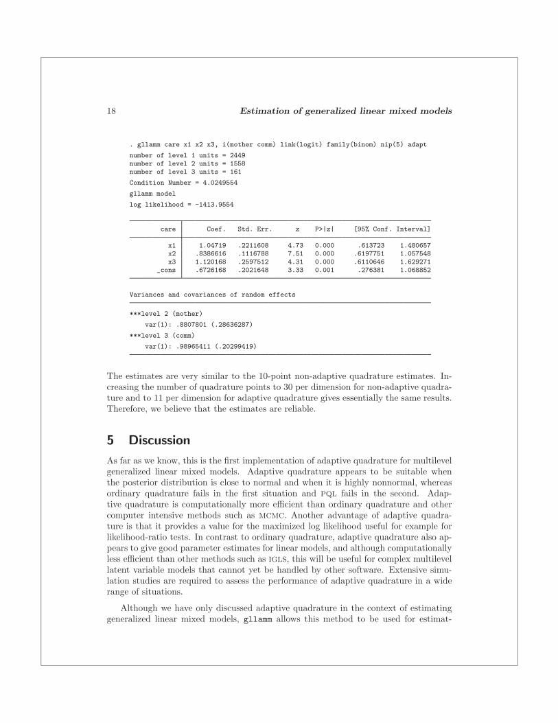
18 Estimation of generalized linear mixed models
. gllamm care x1 x2 x3, i(mother comm) link(logit) family(binom) nip(5) adapt
number of level 1 units = 2449number of level 2 units = 1558number of level 3 units = 161
Condition Number = 4.0249554
gllamm model
log likelihood = -1413.9554
care Coef. Std. Err. z P>|z| [95% Conf. Interval]
x1 1.04719 .2211608 4.73 0.000 .613723 1.480657x2 .8386616 .1116788 7.51 0.000 .6197751 1.057548x3 1.120168 .2597512 4.31 0.000 .6110646 1.629271
_cons .6726168 .2021648 3.33 0.001 .276381 1.068852
Variances and covariances of random effects
***level 2 (mother)
var(1): .8807801 (.28636287)
***level 3 (comm)
var(1): .98965411 (.20299419)
The estimates are very similar to the 10-point non-adaptive quadrature estimates. In-creasing the number of quadrature points to 30 per dimension for non-adaptive quadra-ture and to 11 per dimension for adaptive quadrature gives essentially the same results.Therefore, we believe that the estimates are reliable.
5 Discussion
As far as we know, this is the first implementation of adaptive quadrature for multilevelgeneralized linear mixed models. Adaptive quadrature appears to be suitable whenthe posterior distribution is close to normal and when it is highly nonnormal, whereasordinary quadrature fails in the first situation and PQL fails in the second. Adap-tive quadrature is computationally more efficient than ordinary quadrature and othercomputer intensive methods such as MCMC. Another advantage of adaptive quadra-ture is that it provides a value for the maximized log likelihood useful for example forlikelihood-ratio tests. In contrast to ordinary quadrature, adaptive quadrature also ap-pears to give good parameter estimates for linear models, and although computationallyless efficient than other methods such as IGLS, this will be useful for complex multilevellatent variable models that cannot yet be handled by other software. Extensive simu-lation studies are required to assess the performance of adaptive quadrature in a widerange of situations.
Although we have only discussed adaptive quadrature in the context of estimatinggeneralized linear mixed models, gllamm allows this method to be used for estimat-

S. Rabe-Hesketh, A. Skrondal, and A. Pickles 19
ing general multilevel latent variable models, including multilevel factor models andmultilevel structural equation models; see Rabe-Hesketh et al. (2002). In addition tocounts and dichotomous outcomes, gllamm can handle continuous, censored, ordinal,and nominal responses and rankings, see Skrondal and Rabe-Hesketh (2002), as well ascontinuous and discrete time survival data, see Rabe-Hesketh et al. (2001d).
A problem with gllamm is that it can be very slow, particularly if the models includemany random effects. This is partly because gllamm is written in ado code, which needsto be interpreted by Stata while the program is running. Fortunately, Stata Corporationis converting parts of gllamm to internal code, which should result in a considerableincrease in speed.
6 ReferencesAlbert, P. S. and D. A. Follmann. 2000. Modeling repeated count data subject to
informative dropout. Biometrics 56: 667–677.
Bock, R. D., R. Gibbons, S. G. Shilling, E. Muraki, D. T. Wilson, and R. Wood. 1999.TESTFACT: Test Scoring, Item Statistics, and Full Information Item Factor Analysis.Chicago, IL: Scientific Software International.
Bock, R. D. and S. Schilling. 1997. High-dimensional full-information item factor anal-ysis. In Latent Variable Modelling and Applications to Causality, ed. M. Berkane,164–176. New York: Springer-Verlag.
Breslow, N. E. and D. G. Clayton. 1993. Approximate inference in generalized linearmixed models. Journal of the American Statistical Association 88: 9–25.
Breslow, N. E. and X. Lin. 1995. Bias correction in generalised linear mixed modelswith a single component of overdispersion. Biometrika 82: 81–91.
Browne, W. J. and D. Draper. 2002. A comparison of Bayesian and likelihood methodsfor fitting multilevel models. Submitted.
Bryk, A. S., S. W. Raudenbush, and R. Congdon. 1996. HLM. Hierarchical Linear andNonlinear Modeling with the HLM/2L and HLM/3L Programs. Chicago: ScientificSoftware International.
Carlin, B. P. and T. A. Louis. 1998. Bayes and Empirical Bayes Methods for DataAnalysis. Boca Raton: Chapman & Hall/CRC.
Crouch, E. A. C. and D. Spiegelman. 1990. The evaluation of integrals of the form∫f(t) exp(−t2)dt: Application to logistic-normal models. Journal of the American
Statistical Association 85: 464–469.
Goldstein, H. 1995. Multilevel Statistical Models. London: Arnold.
Goldstein, H. and J. Rasbash. 1996. Improved approximations for multilevel models withbinary responses. Journal of the Royal Statistical Society, Series A 159: 505–513.
20 Estimation of generalized linear mixed models
Goldstein, H., J. Rasbash, I. Plewis, D. Draper, W. Browne, M. Yang, G. Woodhouse,and M. Healy. 1998. A User’s Guide to MLwiN. London: Multilevel Models Project,Institute of Education, University of London.
Hedeker, D. and R. D. Gibbons. 1996. MIXOR: a computer program for mixed-effectsordinal probit and logistic regression analysis. Computer Methods and Programs inBiomedicine 49: 157–176.
Keane, M. P. 1992. A note on identification in the multinomial probit model. Journalof Business and Economic Statistics 10: 193–200.
Lesaffre, E. and B. Spiessens. 2001. On the effect of the number of quadrature pointsin a logistic random-effects model: an example. Applied Statistics 50: 325–335.
Lillard, L. A. and C. W. A. Panis. 2000. Multiprocess Multilevel Modelling, aML Release1, User’s Guide and Reference Manual. Los Angeles: EconoWare.
Lin, X. and N. E. Breslow. 1995. Analysis of correlated binomial data in logistic-normalmodels. Journal of Statistical Computing and Simulation 55: 133–146.
Liu, Q. and D. A. Pierce. 1994. A note on Gauss-Hermite quadrature. Biometrika 81:624–629.
McCullagh, P. and J. A. Nelder. 1989. Generalized Linear Models. 2d ed. London:Chapman and Hall.
McCulloch, C. E. and A. F. M. Searle. 2001. Generalized, Linear and Mixed Models.New York: John Wiley & Sons.
Naylor, J. C. and A. F. M. Smith. 1982. Applications of a method for the efficientcomputation of posterior distributions. Applied Statistics 31: 214–225.
Pinheiro, J. C. and D. M. Bates. 1995. Approximations to the log-likelihood function inthe nonlinear mixed-effects model. Journal of Computational Graphics and Statistics4: 12–35.
Rabe-Hesketh, S., A. Pickles, and A. Skrondal. 2001a. GLLAMM: A general class ofmultilevel models and a Stata program. Multilevel Modelling Newsletter 13: 17–23.
—. 2001b. GLLAMM Manual. London: Tech. Rep. 2001/01, Department of Biostatisticsand Computing, Institute of Psychiatry, King’s College, University of London.http://www.iop.kcl.ac.uk/iop/departments/biocomp/programs/gllamm.html
Rabe-Hesketh, S., A. Pickles, and C. Taylor. 2000. sg129: Generalized linear latentand mixed models. Stata Technical Bulletin 53: 47–57. In Stata Technical BulletinReprints, vol. 9, 293–307. College Station, TX: Stata Press.
Rabe-Hesketh, S., A. Skrondal, and A. Pickles. 2002. Generalized multilevel structuralequation modelling. Submitted.

S. Rabe-Hesketh, A. Skrondal, and A. Pickles 21
Rabe-Hesketh, S., T. Touloupulou, and R. M. Murray. 2001c. Multilevel modelingof cognitive function in schizophrenics and their first degree relatives. MultivariateBehavioral Research. 36: 279–298.
Rabe-Hesketh, S., S. Yang, and A. Pickles. 2001d. Multilevel models for censored andlatent responses. Statistical Methods in Medical Research. 10: 409–427.
Rodriguez, B. and N. Goldman. 1995. An assessment of estimation procedures formultilevel models with binary responses. Journal of the Royal Statistical Society,Series A 158: 73–89.
—. 2001. Improved estimation procedures for multilevel models with binary response:a case study. Journal of the Royal Statistical Society, Series A 164: 339–355.
Skrondal, A. and S. Rabe-Hesketh. 2002. Multilevel logistic regression for polytomousdata and rankings. Submitted.
Spiegelhalter, D., A. Thomas, N. Best, and W. Gilks. 1996. BUGS 0.5 Bayesian Analysisusing Gibbs sampling. Manual (version ii). London: Cambridge: MRC-BiostatisticsUnit.http://www.mrc-bsu.cam.ac.uk/bugs/documentation/contents.shtml
Stryhn, H., I. Dohoo, E. Tillard, and T. Hagedorn-Olsen. 2000. Simulation as a tool ofvalidation in hierarchical generalized linear models. In International Symposium onVeterinary Epidemiology and Economics, 1136–1138. Beckenridge, CO.
Thall, P. F. and S. C. Vail. 1990. Some covariance models for longitudinal count datawith overdispersion. Biometrics 46: 657–671.
Wolfinger, R. D. 1999. Fitting nonlinear mixed models with the new NLMIXED proce-dure. In Proceedings of the 24th SAS User’s Group Meeting. Cary, NC: SAS Institute,Inc.
About the Authors
Sophia Rabe-Hesketh is Senior Lecturer in Statistics at the Department of Biostatistics andComputing, Institute of Psychiatry, King’s College London.
Anders Skrondal is Senior Biostatistician at the Department of Epidemiology, National Insti-tute of Public Health, Oslo.
Andrew Pickles is Professor of Epidemiological and Social Statistics at the School of Epidemi-ology and Health Science and the Cathy Marsh Centre for Census and Survey Research, TheUniversity of Manchester.