rf coil system design for mri applications in ...teorik olarak hesaplanan manyetik alan ile...

RF COIL SYSTEM DESIGN FOR MRI APPLICATIONS ININHOMOGENEOUS MAIN MAGNETIC FIELD

A THESIS SUBMITTED TOTHE GRADUATE SCHOOL OF NATURAL AND APPLIED SCIENCES

OFMIDDLE EAST TECHNICAL UNIVERSITY

BY

AYHAN OZAN YILMAZ

IN PARTIAL FULFILLMENT OF THE REQUIREMENTSFOR

THE DEGREE OF MASTER OF SCIENCEIN

ELECTRICAL AND ELECTRONICS ENGINEERING

JUNE 2007

Approval of the Graduate School of Natural and Applied Sciences.

Prof. Dr. Canan OzgenDirector

I certify that this thesis satisfies all the requirements as a thesis for the degreeof Master of Science.

Prof. Dr. Ismet ErkmenHead of Department

This is to certify that we have read this thesis and that in our opinion it isfully adequate, in scope and quality, as a thesis for the degree of Master ofScience.

Prof. Dr. B. Murat EyubogluSupervisor

Examining Committee Members

Prof. Dr. Nevzat Guneri Gencer (METU, EE)

Prof. Dr. B. Murat Eyuboglu (METU, EE)

Associate Prof. Sencer Koc (METU, EE)

Assistant Prof. Yesim Serinagaoglu (METU, EE)

Prof. Dr. Ergin Atalar (Bilkent, EE)

I hereby declare that all information in this document has been obtained and

presented in accordance with academic rules and ethical conduct. I also declare

that, as required by these rules and conduct, I have fully cited and referenced

all material and results that are not original to this work.

Name, Last name :

Signature :

iii

ABSTRACT

RF COIL SYSTEM DESIGN FOR MRI APPLICATIONS IN

INHOMOGENEOUS MAIN MAGNETIC FIELD

Yilmaz, Ayhan Ozan

Ms, Department of Electrical and Electronics Engineering

Supervisor: Prof. Dr. B. Murat Eyuboglu

June 2007, 146 pages

In this study, RF coil geometries are designed for MRI applications using in-

homogeneous main magnetic fields. The current density distributions that can

produce the desired RF magnetic field characteristics are obtained on prede-

fined cubic, cylindrical and planar surfaces and Tikhonov, CGLS, TSVD and

Rutisbauer regularization methods are applied to match the desired and gen-

erated magnetic fields. The conductor paths, which can produce the current

density distribution calculated for each surface selection and regularization

technique, are determined using stream functions. The magnetic fields gen-

erated by the current distributions are calculated and the error percentages

between the desired and generated magnetic fields are found. Optimum con-

ductor paths that are going to be produced on cubic, cylindrical and planar

surfaces and the required regularization method are determined on the basis

of error percentages and realizability of the conductor paths.

The optimum conductor path calculated for the planar coil is realized and

in the measurement done by LakeShore 3-Channel Gaussmeter, an average

iv

error percentage of 11 is obtained between the theoretical and measured mag-

netic field. The inductance values of the realized RF coil are measured; the

tuning and matching capacitance values are calculated and the frequency char-

acteristics of the system is tested using Electronic Workbench 5.1. The quality

factor value of the tested system is found to be 162.5, which corresponds to a

bandwidth of 39.2 KHz at 6.387 MHz (operating frequency of METU MRI

system).

The techniques suggested in this study can be used in order to design and

realize RF coils on predefined arbitrary surfaces for inhomogeneous main mag-

netic fields. In addition, a hand held MRI device can be manufactured which

uses a low cost permanent magnet to provide a magnetic field and generates

the required RF field with the designed RF coil using the techniques suggested

in this study.

Keywords: Magnetic Resonance Imaging, Rf Coil Design, Inhomogeneous

Main Magnetic Field, Rf Field, Stream Functions, Basis Functions, Method of

Moments, Surface Current Density

v

OZ

HOMOJEN OLMAYAN ANA MANYETIK ALANDA MANYETIK

REZONANS GORUNTULEME ICIN RF SARGISI SISTEMI TASARIMI

Yilmaz, Ayhan Ozan

Yuksek Lisans, Elektrik ve Elektronik Muhendisligi Bolumu

Tez Yoneticisi: Prof. Dr. B. Murat Eyuboglu

Haziran 2007, 146 sayfa

Bu calısmada, homojen olmayan ana manyetik alanlarda kullanılmak uzere

RF sargısı geometrileri tasarlanmıstır. Istenen RF manyetik alan karakterini

olusturabilecek akım yogunlugu dagılımı, onceden tanımlanmıs kubik, silindirik

ve duzlemsel yuzeylerde Momentler Yontemi kullanılarak elde edilmis, elde

edilen akım yogunlugu dagılımlarının yarattıgı manyetik alanın istenen alana

yaklastırılması icin Tikhonov, CGLS, TSVD ve Rutisbauer duzenlilestirme

yontemleri uygulanmıs, her bir yuzey secimi ve duzenlilestirme yontemi icin

hesaplanan akım yogunlugunu olusturabilecek iletken sekilleri Akı Fonksiy-

onları kullanılarak belirlenmistir. Elde edilen akım yogunlugu dagılımlarının

olusturdugu manyetik alanlar hesaplanmıs, hesaplanan alanlar ile olusturulmak

istenen alanlar arasındaki hata yuzdeleri hesaplanmıstır. Hata yuzdeleri ve

iletken sekillerinin hayata gecirilebilme kolaylıgı goz onunde bulundurularak;

silindirik, kubik ve duzlemsel yuzeyler uzerine yerlestirilmek uzere optimum

iletken sekilleri belirlenmis, bu sekilleri elde etmek icin kullanılması gereken

duzenlilestirme yontem ve parametreleri belirlenmistir.

vi

Elde edilen sonuclardan duzlemsel yuzey icin hesaplanan iletken sekli gerceklestirilmis,

teorik olarak hesaplanan manyetik alan ile LakeShore 3 Kanallı Gaussmetre

kullanılarak olculen manyetik alan arasında 11 ortalama hata yuzdesi elde

edilmistir. Gerceklestirilen RF sargısının induktans degerleri olculmus, ayarlama

ve esleme kapasitor degerleri hesaplanmıs, Electronic Workbench 5.1 kullanılarak

elde edilen sistem test edilmistir. Test edilen sistemin kalite faktor degeri 162.5

olarak belirlenmistir. Bu deger 6.387 MHz’te (ODTU MRG sistemi calısma

frekansı) 39.2 KHz’lik bir bant genisligine karsılık gelmektedir.

Bu calısmada onerilen teknikler kullanılarak homojen olmayan bir ana manyetik

alanda kullanılabilecek RF sargıları, onceden tanımlanmıs yuzeyler uzerinde

tasarlanıp gerceklestirilebilir. Ayrıca gelistirilen sargı sayesinde kalıcı mıknatıs

ile yaratılan manyetik alanlar kullanılarak elde uygulanabilecek tasınabilir bir

manyetik rezonans goruntuleme cihazı tasarlanabilir.

Anahtar Kelimeler: Manyetik Rezonans Goruntuleme, Rf Sargısı Tasarımı,

Homojen Olmayan Ana Manyetik Alan, RF Alanı, Akı Fonksiyonları, Taban

Fonsiyonları, Momentler Yontemi, Yuzey Akım Yogunlugu

vii

To my father,

viii

ACKNOWLEDGMENTS

I would like to express my profound gratitude to my advisor Prof. Dr. Murat

Eyuboglu for his guidance and support throughout this study.

I owe much to my friend Volkan Emre Arpınar, who is a great hero saving

people that get stuck in problems, for his help in my progress throughout my

studies. I thank Evren Degirmenci and Dario Martin Lorca for their motiva-

tion and mental support. Thanks to Mustafa Secmen for his help to construct

the coil and to Zekeriya Ozgun for his help to construct the experimental

setup. I would also like to thank Hus, Doga, Taha and Koray for being to-

gether throughout the way.

I feel grateful to my family for giving me the heart and mind to overcome

the difficulties and all the situations I have faced.

I was so lucky to have the support of Dilek, concon butterfly, and Dunc,

Aysegul, the guvercin; and the cakes and boreks of Nihal Teyze on hard days.

Also thanks to Aero for manufacturing the air bed I used for several nights

though for the last few days the air lasted only for three hours. On the overall,

it was bliss to serve for a purpose that provides progress in health occasions.

I hope I could perform a few paces towards the health and comfort of human

beings.

ix

TABLE OF CONTENTS

ABSTRACT . . . . . . . . . . . . . . . . . . . . . . . . . . . . . . . . . iv

OZ . . . . . . . . . . . . . . . . . . . . . . . . . . . . . . . . . . . . . . . vi

DEDICATION . . . . . . . . . . . . . . . . . . . . . . . . . . . . . . . . viii

ACKNOWLEDGMENTS . . . . . . . . . . . . . . . . . . . . . . . . . . viii

TABLE OF CONTENTS . . . . . . . . . . . . . . . . . . . . . . . . . . x

LIST OF TABLES . . . . . . . . . . . . . . . . . . . . . . . . . . . . . . xiii

LIST OF FIGURES . . . . . . . . . . . . . . . . . . . . . . . . . . . . . xv

CHAPTER

1 INTRODUCTION . . . . . . . . . . . . . . . . . . . . . . . . . 1

1.1 Background . . . . . . . . . . . . . . . . . . . . . . . . . 6

1.2 Objectives of the Thesis . . . . . . . . . . . . . . . . . . 9

1.3 Outline of the Thesis . . . . . . . . . . . . . . . . . . . 10

2 RF Coil Design in Inhomogeneous Main Fields Using Methodof Moments . . . . . . . . . . . . . . . . . . . . . . . . . . . . . 11

2.1 Method of Moments (MoM) . . . . . . . . . . . . . . . . 11

2.1.1 A General Solution Procedure . . . . . . . . . 12

2.2 Maxwell Relations . . . . . . . . . . . . . . . . . . . . . 13

2.3 Combining MoM and Maxwell Relations . . . . . . . . . 15

2.4 Regularization . . . . . . . . . . . . . . . . . . . . . . . 18

2.4.1 The Idea of Regularization . . . . . . . . . . . 21

2.5 Stream Functions . . . . . . . . . . . . . . . . . . . . . 21

3 Implementing the Coil Structure by Using Regularization Meth-ods and Stream Functions . . . . . . . . . . . . . . . . . . . . . 26

3.1 Defining the Required Magnetic Field . . . . . . . . . . 26

3.1.1 RF Field Case 1 . . . . . . . . . . . . . . . . . 28

x

3.1.2 RF Field Case 2 . . . . . . . . . . . . . . . . . 29

3.1.3 RF Field Case 3 . . . . . . . . . . . . . . . . . 31

3.1.4 RF Field Case 4 . . . . . . . . . . . . . . . . . 31

3.2 Defining Target and Source Fields . . . . . . . . . . . . 33

3.2.1 Cylindrical Source Surface . . . . . . . . . . . 34

3.2.2 Tri-Planar Source Surface . . . . . . . . . . . . 35

3.2.3 Planar Source Surface . . . . . . . . . . . . . . 37

3.2.4 Orthogonal Three Planes . . . . . . . . . . . . 38

3.3 Defining the Basis Functions . . . . . . . . . . . . . . . 39

3.3.1 Basis Functions for Cylindrical Geometry . . . 40

3.3.1.1 Stream Functions . . . . . . . . . . 42

3.3.2 Basis Functions for Planar Geometries . . . . . 43

3.3.2.1 Stream Functions . . . . . . . . . . 47

3.4 Forming the Matrix Equation . . . . . . . . . . . . . . . 48

3.4.1 Magnetic Field Expressions . . . . . . . . . . . 48

3.4.2 Method . . . . . . . . . . . . . . . . . . . . . . 50

3.5 Obtaining the Solution by Regularization . . . . . . . . 53

3.6 Approximating the Stream Function by a Conductor . . 54

3.6.1 A simple Procedure . . . . . . . . . . . . . . . 54

4 Results and Conclusion . . . . . . . . . . . . . . . . . . . . . . . 56

4.1 Theoretical Results . . . . . . . . . . . . . . . . . . . . 57

4.1.1 Desired and Generated Magnetic Fields . . . . 57

4.1.2 Stream Function Contours . . . . . . . . . . . 59

4.2 Realizing the Coil . . . . . . . . . . . . . . . . . . . . . 68

4.2.1 Orientation of Field Points . . . . . . . . . . . 68

4.2.2 Implementation of the Planar Coil . . . . . . . 70

4.2.2.1 Current Density and Stream Func-tion Solutions . . . . . . . . . . . . 70

4.2.2.2 Comparing the Desired, Generatedand Measured Fields . . . . . . . . 74

4.2.2.3 Constructing the Coil and the Cir-cuitry . . . . . . . . . . . . . . . . 76

4.2.3 Tuning and Matching the RF Coil . . . . . . . 85

4.3 Conclusion . . . . . . . . . . . . . . . . . . . . . . . . . 90

xi

4.4 Future Work . . . . . . . . . . . . . . . . . . . . . . . . 92

5 Publications . . . . . . . . . . . . . . . . . . . . . . . . . . . . . 93

5.1 Publications Prior to M. Sc. Study . . . . . . . . . . . . 93

5.2 Publications during M. Sc. Study . . . . . . . . . . . . . 93

REFERENCES . . . . . . . . . . . . . . . . . . . . . . . . . . . . . . . . 94

APPENDICES . . . . . . . . . . . . . . . . . . . . . . . . . . . . . . . . 99

A Regularization . . . . . . . . . . . . . . . . . . . . . . . . . . . . 99

A.1 Singular Value Decomposition . . . . . . . . . . . . . . . 99

A.2 The Generalized Singular Value Decomposition (GSVD) 100

A.3 QR Decomposition . . . . . . . . . . . . . . . . . . . . . 101

A.3.1 Householder Transformation . . . . . . . . . . 101

A.3.2 Givens Rotations . . . . . . . . . . . . . . . . 103

A.4 Orthogonal Bidiagonalization . . . . . . . . . . . . . . . 105

A.5 Direct Regularization Techniques . . . . . . . . . . . . . 107

A.5.1 Tikhonov Regulatization . . . . . . . . . . . . 107

A.5.1.1 Least Squares with a Quadratic Con-straint . . . . . . . . . . . . . . . . 111

A.5.1.2 Inequality or Equality Constraints . 111

A.5.1.3 Related Methods . . . . . . . . . . 113

A.5.2 The Regularized General Gauss-Markov Lin-ear Model . . . . . . . . . . . . . . . . . . . . 115

A.5.2.1 Numerical Algorithm . . . . . . . . 117

A.5.2.1.1 Step1 . . . . . . . . . . . . . . . 118

A.5.2.1.2 Step2 . . . . . . . . . . . . . . . 118

A.5.2.1.3 Step3 . . . . . . . . . . . . . . . 118

A.5.3 Truncated SVD and GSVD (TSVD and TGSVD)119

A.5.4 Algorithms based on Total Least Squares . . . 120

A.5.4.1 Truncated Total Least Squares (TTLS)120

A.5.4.2 Regularized TLS (R-TLS) . . . . . 121

A.5.5 Other Direct Methods . . . . . . . . . . . . . . 123

A.6 Iterative Regularization Methods . . . . . . . . . . . . . 127

A.6.1 Landweber Iteration . . . . . . . . . . . . . . . 127

A.6.2 Regularizing Conjugate Gradient(CG) Iterations127

xii

LIST OF TABLES

3.1 Parameters in the basis function definition for cylindrical surface 40

3.2 Basis function characteristics for Cylindrical Surface varyingp, q, H1 and H2 - 1 . . . . . . . . . . . . . . . . . . . . . . . . 41

3.3 Basis function characteristics for Cylindrical Surface varyingp, q, H1 and H2 - 2 . . . . . . . . . . . . . . . . . . . . . . . . 42

3.4 Parameters in the basis function definition for planar surfaces 44

3.5 Basis function characteristics for planar geometries varying p,q, H1 and H2 - 1 . . . . . . . . . . . . . . . . . . . . . . . . . 45

3.6 Basis function characteristics for planar geometries varying p,q, H1 and H2 - 2 . . . . . . . . . . . . . . . . . . . . . . . . . 46

3.7 Mapping for u and v parameters onto Cartesian coordinates . 47

4.1 Error percentages for solutions with minimum error. Min-imum error percentages between the desired and generatedmagnetic field are illustrated for the current density solutionsobtained by applying the regularization methods listed as columnsto source surfaces listed as rows for the corresponding targetfields. . . . . . . . . . . . . . . . . . . . . . . . . . . . . . . . . 57

4.2 Error percentages for solutions with optimum error. Error per-centages between the desired and generated magnetic field areillustrated for the optimum current density solutions obtainedby applying the regularization methods listed as columns tosource surfaces listed as rows for the corresponding target fields. 57

4.3 Regularization parameter values for planar surface . . . . . . . 58

4.4 Regularization parameter values for tri-planar surface . . . . . 58

4.5 Regularization parameter values for three orthogonal planes . . 59

4.6 Regularization parameter values for cylindrical surface . . . . . 59

4.7 Stream function contours for planar surface - 1 . . . . . . . . . 60

4.8 Stream function contours for planar surface - 2 . . . . . . . . . 61

4.9 Stream function contours for tri-planar surface - 1 . . . . . . . 62

4.10 Stream function contours for tri-planar surface - 2 . . . . . . . 63

4.11 Stream function contours for three orthogonal planes - 1 . . . 64

4.12 Stream function contours for three orthogonal planes - 2 . . . 65

4.13 Stream function contours for cylindrical surface - 1 . . . . . . 66

4.14 Stream function contours for cylindrical surface - 2 . . . . . . 67

xiii

4.15 Error percentages between desired, calculated and measuredFields . . . . . . . . . . . . . . . . . . . . . . . . . . . . . . . 85

4.16 Inductance values for conductor paths . . . . . . . . . . . . . . 864.17 Tuning and matching parameters for conductor paths . . . . . 86

A.1 Relation between the solutions xα, xα and α value. . . . . . . 123A.2 Relation between the solutions and parameters of the R-TLS

problem. . . . . . . . . . . . . . . . . . . . . . . . . . . . . . . 123

xiv

LIST OF FIGURES

2.1 Equally spaced contours of ψ represent winding patterns withconstant current in each streamline. The difference betweenthe magnitude of ψ2 at point (x2, y2) and the magnitude of ψ1

at point (x1, y1) is equal to the magnitude of the current I12

flowing between the streamlines ψ1 and ψ2. . . . . . . . . . . . 23

3.1 Main magnetic field Vectors in the field volume. A square wireof 10cm by 10cm is considered on yz-plane. The center of thesquare coil is at point (0,0,0) and the coil generates magneticfield vectors represented by the arrows of length proportionalto the magnitudes at every field point. . . . . . . . . . . . . . 27

3.2 Main magnetic field and RF field vectors within the field vol-ume for case 1. The main magnetic field vectors are illustratedas blue arrows, while RF field vectors are illustrated as red ar-rows. . . . . . . . . . . . . . . . . . . . . . . . . . . . . . . . . 29



3.5 Main magnetic field and RF field vectors within the field vol-ume for case 4. The main magnetic field vectors are illustratedas blue arrows, while RF field vectors are illustrated as red ar-rows. RF Field vector magnitudes are scaled by a factor of0.5. . . . . . . . . . . . . . . . . . . . . . . . . . . . . . . . . . 33

3.6 Target and source fields for cylindrical surface problem defini-tion.The cube inside the cylinder is the target field while thecylindrical surface is the source field. . . . . . . . . . . . . . . 34

3.7 Spatial mapping of cylinder surface coordinates onto subdo-mains. . . . . . . . . . . . . . . . . . . . . . . . . . . . . . . . 35

xv

3.8 Target and source fields for tri-planar surface problem defini-tion. The cube in front of the tri-planar geometry is the targetfield while the tri-planar surface is the source field. . . . . . . . 36

3.9 Spatial mapping of tri-planar surface coordinates onto subdo-mains. . . . . . . . . . . . . . . . . . . . . . . . . . . . . . . . 37

3.10 Target and source fields for planar surface problem defini-tion.The cube in front of the planar geometry is the targetfield while the planar surface is the source field. . . . . . . . . 38

3.11 Target and source fields for orthogonal three planes problemdefinition.The cube in the middle of the three planes is thetarget field while the three orthogonal planes form the sourcefield. . . . . . . . . . . . . . . . . . . . . . . . . . . . . . . . . 39

4.1 Stream function contours on the cylindrical surface for thesolution with optimum error . . . . . . . . . . . . . . . . . . . 68

4.2 Orientation of field points in the target field. The target fieldis made up of 1800 field points. The target volume is a 10 cmby 10 cm by 10 cm cube the center of which is placed at point(0,12.5,0) and which is divided into 15, 8 and 15 divisions inx, y and z directions respectively.During the formation of fieldpoints, first the x- axis is filled while y and z values are keptconstant. When a single x row is filled, which corresponds to15 points, z value is incremented and another x row is filledfrom negative to positive direction. This means, the purpledot corresponds to “1” on the magnetic field plot and thefirst 15 point group on the magnetic field plot symbolize thehighlighted points in Figure 4.2, increasing in value in thedirection of the green arrows on Figure 4.2. When a singleslice of the cube is filled, which corresponds to 225 points, yvalue is incremented . . . . . . . . . . . . . . . . . . . . . . . . 69

4.3 Normalized desired magnetic field Components at field points.The first 1800 field points correspond to the x-component ofthe magnetic field with the orientation stated above. Thesecond and third 1800 field points correspond to the y and zcomponents respectively. . . . . . . . . . . . . . . . . . . . . . 70

4.4 Magnitude of Jx solution for the planar surface on xz-plane.The center of the planar surface of dimensions 30 cm by 30cm is placed at (x=0, z=0) on xz-plane. The magnitude of Jis expressed in A/m. . . . . . . . . . . . . . . . . . . . . . . . 71

4.5 Magnitude of Jz solution for the planar surface on xz-plane.The center of the planar surface of dimensions 30 cm by 30cm is placed at (x=0, z=0) on xz-plane. The magnitude of Jis expressed in A/m. . . . . . . . . . . . . . . . . . . . . . . . 71

4.6 Current density distribution solution on the planar surfaceon xz-plane in vector form. The lengths of the arrows areproportional to the magnitude of the current density vector atthe corresponding point. . . . . . . . . . . . . . . . . . . . . . 72

xvi

4.7 Stream function solution for the current density distributionon the xz-plane. x and z axis represent the coordinates of thepoints on the planar surface in meters. The stream functionis represented with 25 streamlines. . . . . . . . . . . . . . . . . 73

4.8 Streamlines for the stream function solution on the xz-Plane.x and z axis represent the coordinates of the points on theplanar surface in meters. The stream function is representedwith 6 streamlines. . . . . . . . . . . . . . . . . . . . . . . . . 74

4.9 Normalized magnetic field components generated by currentdensity solution. The first 1800 field points correspond to thex-component of the magnetic field with the orientation statedin the text. The second and third 1800 field points correspondto the y and z components respectively. . . . . . . . . . . . . . 75

4.10 Normalized magnetic field components generated using stream-lines. Streamlines are considered as conductor wires. The first1800 field points correspond to the x-component of the mag-netic field with the orientation stated above. The second andthird 1800 field points correspond to the y and z componentsrespectively. . . . . . . . . . . . . . . . . . . . . . . . . . . . . 76

4.11 Planar RF coil design. Each conductor path is representedas an independent wire strip. The wires that carry the samecurrent magnitudes are interconnected. . . . . . . . . . . . . . 77

4.12 Realized RF coil. The wires that carry the same current mag-nitudes are interconnected. The wire strips labeled as 1a-1b-6-8; 3-4; 2a-2b-5-9; 7 form four independent current paths. . . 78

4.13 Circuit to provide DC currents. The currents to feed the RFcoil wire are obtained by the emitter currents of each branch. . 79

4.14 Experimental setup for the measurements. Two parallel platesare placed on four rods and the height of the plates are deter-mined by screws on each rod. . . . . . . . . . . . . . . . . . . 81

4.15 Normalized measured magnetic field - Measurement 1. y-component of the magnetic field is measured using the LakeShore3-Channel Gaussmeter. The target volume is a cube of dimen-sions 3.3cm by 3.3cm by 3.3cm. The target volume is dividedinto 5, 8 and 5 divisions in x, y and z directions respectivelyyielding 200 field points . . . . . . . . . . . . . . . . . . . . . . 82

4.16 Normalized measured magnetic field - Measurement 2. Sec-ond measurement is done on the y-component of the magneticfield using the LakeShore 3-Channel Gaussmeter under similarconditions. . . . . . . . . . . . . . . . . . . . . . . . . . . . . . 83

4.17 Normalized measured magnetic field - Measurement 3. Thirdmeasurement is done on the y-component of the magnetic fieldusing the LakeShore 3-Channel Gaussmeter under similar con-ditions. . . . . . . . . . . . . . . . . . . . . . . . . . . . . . . . 83

xvii

4.18 Calculated magnetic field. y-component of the magnetic fieldis calculated considering the streamlines as conductor paths.The target volume is a cube of dimensions 3.3cm by 3.3cm by3.3cm. The target volume is divided into 5, 8 and 5 divisionsin x, y and z directions respectively yielding 200 field points . 84

4.19 Equivalent circuit diagram for the RF coil . . . . . . . . . . . 874.20 Frequency response of the equivalent circuit. Voltage and

phase of the equivalent circuit are marked for the operatingfrequency. Also the frequency where the power of the equiva-lent circuit is halved is also marked. . . . . . . . . . . . . . . . 88

4.21 Voltage magnitude on the equivalent circuit at the operatingfrequency when the coil is considered to be connected in serieswith a resistance of 50 Ω. At 6.387MHz, the applied voltageof 10V is divided into two; in other words, the coil is matchedto 50 Ω. . . . . . . . . . . . . . . . . . . . . . . . . . . . . . . 89

4.22 The phase of the equivalent circuit at the operating frequencywhen the coil is considered to be connected in series with aresistance of 50 Ω. At 6.387MHz, the phase of the equivalentcircuit is nearly zero; in other words, the coil is tuned to 50 Ω. 89

A.1 Penalty term comparison . . . . . . . . . . . . . . . . . . . . . 126

xviii

CHAPTER 1

INTRODUCTION

Magnetic Resonance imaging is a tomographic imaging technique that pro-

duces images of internal physical and chemical characteristics of an object

from externally measured nuclear magnetic resonance (NMR) signals. The

first successful nuclear magnetic resonance (NMR) experiment was made in

1946 independently by two scientists in the United States. Bloch et al [1, 2]

and Purcell et al [3], found that when certain nuclei were placed in a magnetic

field they absorbed energy in the radio frequency range of the electromagnetic

spectrum, and re-emitted this energy when the nuclei transferred to their orig-

inal state. The strength of the magnetic field and the radio frequency matched

each other as earlier demonstrated by Joseph Larmor and is known as the Lar-

mor relationship.

In 1973, Paul Lauterbur described a new imaging technique [4]. This referred

to the joining together of a weak gradient magnetic field with the stronger main

magnetic field allowing the spatial localization of two test tubes of water. He

used a back projection method to produce an image of the two test tubes. This

imaging experiment moved from the single dimension of NMR spectroscopy to

the second dimension of spatial orientation being the foundation of Magnetic

Resonance Imaging (MRI).

Raymond Damadian demonstrated that a NMR tissue parameter (termed T1

relaxation time) of tumor samples, measured in vitro, was significantly higher

1

than normal tissue. The first whole body image is published by Damadian et

al [5] in 1977.

Clinical MRI uses the magnetic properties of hydrogen and its interaction

with both a large external magnetic field and radio waves to produce highly

detailed images of the human body. Conventional MRI relies upon highly ho-

mogeneous magnetic fields and linear gradient field. In this thesis, designing

RF coils for inhomogeneous fields is studied.

MRI using open imaging systems is discussed in several studies. Balibanu et

al [6] simulated the NMR signal and investigated the effect of pulse sequences

for a hand held NMR-MOUSE (mobile universal surface explorer) composed

of a permanent magnet which was modeled as surface elements and an RF

coil, which was modeled as set of circles.

Anferova et al [7] measured the dead times for NMR signals for an NMR-

MOUSE hardware setup composed of a permanent with two poles, set of

straight wires serving as a gradient coil between the poles, and spiral shaped

RF coil placed parallel to the magnet’s pole surfaces. Casanova and Blumich

[8] obtained a two dimensional image using a similar structure with an addi-

tional gradient field. Improving the study of Casanova and Blumich, Perlo et

al [9] achieved 3D imaging with the single sided sensor.

Blumler et al [10] designed a similar hand held NMR device introducing an

additional sweep coil to enhance the static field of the permanent magnet and

obtained two dimensional images on planes normal to the permanent magnet

pole surface.

All the studies stated above utilized the inhomogeneous magnetic field as the

main magnetic field. However, they either tried to produce a magnetic field as

homogenous as possible or selected a particular region where the main field did

2

not relatively vary. On the contrary, Prado [11] worked in an inhomogeneous

main field without the effort of selecting a relatively homogeneous region and

measured echo signals with a circular RF coil, which he connected to a relay

controlled unit that could switch to different capacitor connections so that the

coil could be tuned to different frequencies matching the magnetic field ampli-

tude values. However, he did not worry about the magnetic field produced by

the coil or obtaining an image by spatial encoding. RF field, in these studies,

are desired to be homogeneous and perpendicular to the main field, but the

concern on RF coils only consisted of forming a coarsely perpendicular field to

the main field by placing the coil on a perpendicular plane in spiral or circular

structures.

While most of the studies on MRI in inhomogeneous fields approach the inho-

mogeneity as a defect to be amended, there are some studies that make use of

the inhomogeneity. Thayer [12] and Yigitler [13] simulated MRI making use

of inhomogeneous main magnetic fields. In Yigitler’s study an inhomogeneous

RF field is used in order to excite the spins and two dimensional images are

obtained by the simulation.

Studies on the optimization of coil shapes are usually carried out for con-

ventional MRI applications. There are two main kinds of RF coils, volume

coils and surface coils. Volume coils include Helmholtz coils, saddle coils, and

birdcage coils. Volume coils can be used as either transmit or receive coils.

The most common RF coil for volume imaging in MRI, is the RF birdcage

coil which encloses the imaged volume allowing open access from the top and

bottom sides. The birdcage coil was first introduced by Hayes et al [14]. The

studies of Tropp [15], [16] on birdcage coils form a basis for RF coil improve-

ments in MRI. Doty et al [17] developed a new class of RF volume coil denoted

as Litz coil, improving the tuning range, homogeneity, tuning stability and

sensitivity compared to birdcage coils. To allow greater access to the imaged

3

volume, it is advantageous to design an RF coil with more open sides, such as

in front as well as top and bottom.

One of the first open RF coils was designed by Roberts et al [18], who used

longitudinal wires on two parallel plates as the coil and obtained images of the

human abdomen in axial and sagittal planes. Open birdcage coils have been

designed by breaking the two end-rings at the zero current points and then

using half of the coil to generate the magnetic field [19], [20]. A U-shaped coil

was also investigated for the different directional modes using the half-birdcage

principle [21]. Alternatively, dome-shaped RF coils have been designed to en-

close only the top half of the imaged volume [22], [23].

Surface coils have high SNR, but a small field of view (FOV). To improve

signal coil design, arrays of surface coils are used [24], [25]. This increases the

FOV without decreasing SNR. In order to improve the quality factor, SNR and

radiation loss of the surface coils, microstrip and high temperature conducting

materials of various alloys have been used for surface coils.

Lee et al [26] used an array of parallel microstrips with a high permittivity

substrate. Zhang et al [27] developed a microstrip spiral coil that reduced the

radiation loss and perturbation of the sample loading to the RF coil compared

to conventional surface coils.

Ma et al [28], [29] developed and fabricated circular High-Temperature Su-

perconductor (HTS) coils made from Y BCO(Y Ba2Cu3O7− Y ttriumbarium

copperoxide) thin films on two inch LaAlO3(LanthanumAluminate) substrates

with chemical etching techniques and achieved better quality factors and im-

age qualities compared to spiral copper coils and volume coils.

Ginefri et al [30] compared a spiral HTS coil made with Y BCO supercon-

ductor on LaAlO3 substrate with copper coil of same shape varying the sizes,

4

temperatures of the coils and size of the sample. They proved a range of 4.1-

11.4 fold improvement in SNR over that obtained with the room-temperature

copper coil.

The open RF coil designs stated above are generally modifications of volume

coils or variations of simple circular, spiral or circular geometries. The coil

shape is usually fixed at the beginning of each study and the variables such as

the materials of coil fabrication, the dimensions of the conductor, the number

of turns for a spiral or size of the gap between conductors are aimed to be

optimized. Also the quantities that are desired to be improved are usually

quality factor and SNR values rather than the magnetic field produced by the

coil.

Using an inverse approach can broaden the limits of the coil design prob-

lem in the sense that the coil shape can be determined based on the desired

quantities rather than determining an initial coil and measuring how close the

quantities are to the desired ones.

One of the first studies that used inverse approach to design coils was per-

formed by Martens et al [31] who designed the conductor contours on two

parallel planes for a gradient coil based on the magnetic field that is desired

to be produced by the coil.

Later Fujita et al [32] extended the inverse approach to optimize wire patterns

of a cylindrical RF coil by quasi-static approach based on SNR and magnetic

field of the coil.

The studies carried out by Lawrence et al [33], [34], While et al [35] and

Muftuler et al [36] obtained current distribution on cylindrical surfaces by

inverse approach, discretized current density using Method of Moments and

obtained conductor patterns using stream functions. The images obtained by

5

Lawrence et al [33], [34] proved averaged SNR and better homogeneity com-

pared to birdcage coils.

This thesis outlines the design of an open RF coil using the time-harmonic

inverse approach, as an extension to and modification of the technique out-

lined in [19]. This method entails the calculation of an ideal current density

on arbitrary surfaces that would generate a specified magnetic field. Different

regularization techniques are used to match the generated magnetic field and

the desired magnetic field. The stream-function technique is used to ascertain

conductor pattern.

The design approach used in this thesis differs from previous designs by using

a modification of the time-harmonic inverse approach to calculate the current

required to generate the specified field. Also, differing from previous designs,

this work aims to design an RF coil that can be utilized in MRI applications

that use an inhomogeneous magnetic field as the main field. Therefore, the

magnetic field that is specified to be generated by the RF coil is required to

be also inhomogeneous.

1.1 Background

A nucleus with a non-zero spin creates a magnetic field around it, which is

analogous to that of a microscopic bar magnet. Physically, this is called nuclear

magnetic dipole moment or magnetic moment. Spin angular momentum ~J and

magnetic moment vectors ~µ are related such that

~µ = γ ~J (1.1)

where γ is a nucleus-dependent physical constant called gyromagnetic ratio.

Although the magnitude of ~µ is constant under any conditions, its direction

is completely random in the absence of an external field. In order to activate

6

macroscopic magnetism from an object, it is necessary to line up the spin

vectors. In conventional MRI, this is accomplished by a strong homogeneous

one directional external magnetic field of strength B0.

~B0 = B0~k (1.2)

where ~k is the unit vector in z direction. According to mechanics, the torque

that ~µ experiences from the external magnetic field is given by ~µ×B0~k which

is equal to rate of change of its angular momentum.

d ~J

dt= ~µ×B0

~k (1.3)

It is concluded that the angular frequency of nuclear precession is

w0 = γB0 (1.4)

which is known as Larmor frequency and precession of ~µ about ~B0 is clockwise

if observed against the direction of the magnetic field [37]. In order for the

spins to produce signals, they should be flipped onto the transverse plane.

This is performed by a rotating RF field, which is perpendicular to the main

magnetic field. For conventional MRI, main magnetic field is in the z direction.

Therefore, the effective RF excitation field is modeled as a field oscillating on

the transverse plane in clockwise direction perpendicular to the main field:

~B1(t) = Be1(t)[cos(wrf t + ϕ)~i− sin(wrf t + ϕ)~j] (1.5)

where Be1(t) is the envelope function, wrf is the carrier frequency and ϕ is the

initial phase angle [37].

The resonance condition for the RF field is that it should rotate in the same

manner as the precessing spins, in other words

wrf = w0 (1.6)

When Bloch Equation for the rotating frame is considered [37] under the as-

sumption that the duration of the RF pulse is short compared to T1 and T2

7

relaxation times, the motion of the bulk magnetization can be expressed as

∂ ~M

∂t= γ ~Mrot ×Be

1(t)~i (1.7)

where ~Mrot is the magnetization vector in rotating frame of reference and γ is

the gyromagnetic ratio.

Under initial conditions Mx′(0) = 0, Mz′(0) = 0, Mz′(0) = M0z , magnetization

vector components at time t can be expressed as

Mx′(t) = 0 (1.8)

My′(t) = M0z sin α (1.9)

Mz′(t) = M0z cos α (1.10)

where

α =

∫ t

0

γBe1(t)dt (1.11)

If a rectangular RF pulse of duration τp is considered, the flip angle is

α = γB1τp (1.12)

which indicates that the flip angle of the magnetization vector is determined

by the duration and strength of the RF pulse. If a linear relation is assumed

between the flip angle and the RF field strength, which is known as small flip

angle approximation [38], then the flip angle of the spins resonating with w of

deviation from wrf is

α(w) =FBe

1(t)(w)

FBe1(t)(0)

α(0) (1.13)

If a rectangular RF pulse of duration τp is considered, spins resonating at a

frequency range of |w−wrf | < 2πτp

are excited by the RF pulse. This indicates

that rectangular pulses with long duration are more selective.

Gradient fields, which are special kinds of inhomogeneous fields that provide

linearly varying magnetic fields along a specific direction, are used to select

8

slices to be excited and to localize spatial data by frequency and phase encod-

ings. In conventional MRI three gradient coils are used in order to provide

varying magnetic fields along x, y and z directions, which make it possible to

excite or localize objects point wise in 3D space.

The main idea in the application of homogeneous main magnetic field and

linearly varying gradient fields in conventional MRI is to align all spins in a

controlled manner and vary the precession frequencies with a known, linearly

changing, controlled inhomogeneity so that spins within slices, strips or points

of a three dimensional object can be discriminated with a relation between

precession frequency and spatial location.

1.2 Objectives of the Thesis

Objectives of this study are listed as follows:

• Determine four arbitrary surfaces which the RF coil is going to be pro-

duced on.

• Model an inhomogeneous main magnetic field and determine the RF field

that is desired to be generated by the coil based on the main field.

• Model the current density and magnetic field relations in the form of

Fredholm integral equations and use inverse approach to obtain current

density distributions on each selected surface.

• Discretize the current density distribution to solve the problem as a ma-

trix equation and use four different regularization techniques to match

the generated magnetic field and the desired magnetic field.

• Obtain current flow paths for each surface selection and regularization

technique using stream functions.

• Calculate the error percentage between the generated and desired mag-

netic field for each surface selection and regularization technique.

9

• Compare the error percentages and current flow paths and determine the

optimum surface and regularization technique so that the error percent-

age is minimum and the current path is realizable.

• Fabricate the optimum planar coil and measure the magnetic field pro-

duced by the coil.

• Simulate the required circuitry to tune and match the coil to operate at

6.378 MHz in order to be used in 0.15 Tesla METU MRI system.

1.3 Outline of the Thesis

A short introduction on existing MRI modalities and a brief background of

MRI principles is presented in Chapter 1. The theory of the methods used in

order to determine the RF coil structure is presented in Chapter 2. The im-

plementation of the methods represented in Chapter 2 is presented in Chapter

3 for the RF coil design problem in inhomogeneous main field using various

target and source field definitions. The experiments carried out based on the

simulations and the results of these experiments and simulations are discussed

in Chapter 4.

10

CHAPTER 2

RF Coil Design in Inhomogeneous Main

Fields Using Method of Moments

This chapter presents the relation between current density and magnetic field

using Maxwell equations and techniques for reducing functional equations to

matrix equations using method of moments. Regularization methods are in-

troduced in order to solve ill-conditioned matrix equations formed by method

of moments. Finally, stream functions are represented, which are used to de-

termine current paths for current density solution.

2.1 Method of Moments (MoM)

MoM is used to provide a unified treatment of matrix methods for comput-

ing the solutions to field problems. The basic idea is to reduce a functional

equation to a matrix equation, and then solve the matrix equation by known

techniques. These concepts are best expressed as linear spaces and operators

[39]. For this study, inhomogeneous type of equations,

L(f) = g (2.1)

are considered, where L is a linear operator, g is the source or excitation (known

function), and f is the field or response (unknown function to be determined).

By the term deterministic we mean that the solution to (2.1) is unique; that

is, only one f is associated with a given g. A problem of analysis involves the

11

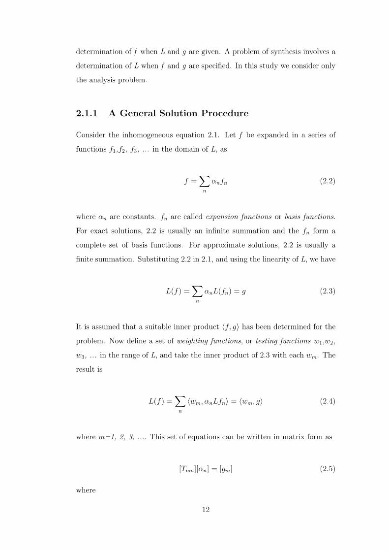
determination of f when L and g are given. A problem of synthesis involves a

determination of L when f and g are specified. In this study we consider only

the analysis problem.

2.1.1 A General Solution Procedure

Consider the inhomogeneous equation 2.1. Let f be expanded in a series of

functions f1,f2, f3, ... in the domain of L, as

f =∑

n

αnfn (2.2)

where αn are constants. fn are called expansion functions or basis functions.

For exact solutions, 2.2 is usually an infinite summation and the fn form a

complete set of basis functions. For approximate solutions, 2.2 is usually a

finite summation. Substituting 2.2 in 2.1, and using the linearity of L, we have

L(f) =∑

n

αnL(fn) = g (2.3)

It is assumed that a suitable inner product 〈f, g〉 has been determined for the

problem. Now define a set of weighting functions, or testing functions w1,w2,

w3, ... in the range of L, and take the inner product of 2.3 with each wm. The

result is

L(f) =∑

n

〈wm, αnLfn〉 = 〈wm, g〉 (2.4)

where m=1, 2, 3, .... This set of equations can be written in matrix form as

[Tmn][αn] = [gm] (2.5)

where

12

[Tmn] =

〈w1, Lf1〉〈w1, Lf2〉 ... 〈w1, Lfn〉〈w2, Lf1〉〈w2, Lf2〉 ... 〈w2, Lfn〉

......

. . ....

〈wm, Lf1〉〈wm, Lf2〉 ... 〈wm, Lfn〉

(2.6)

[αn] =

α1

α2

...

αn

(2.7)

[gm] =

〈w1, g〉〈w2, g〉

...

〈wm, g〉

(2.8)

If the matrix [T ] is nonsingular its inverse [T−1] exists. The αn are then given

by

[αn] = [T−1mn][gm] (2.9)

and the solution for f is given by 2.2.

2.2 Maxwell Relations

The four differential equations that are valid in every point in space for linear,

non-magnetic, isotropic medium are

∇× ~E = −∂ ~B

∂t(2.10)

∇× ~H = ~Js +∂ ~D

∂t(2.11)

13

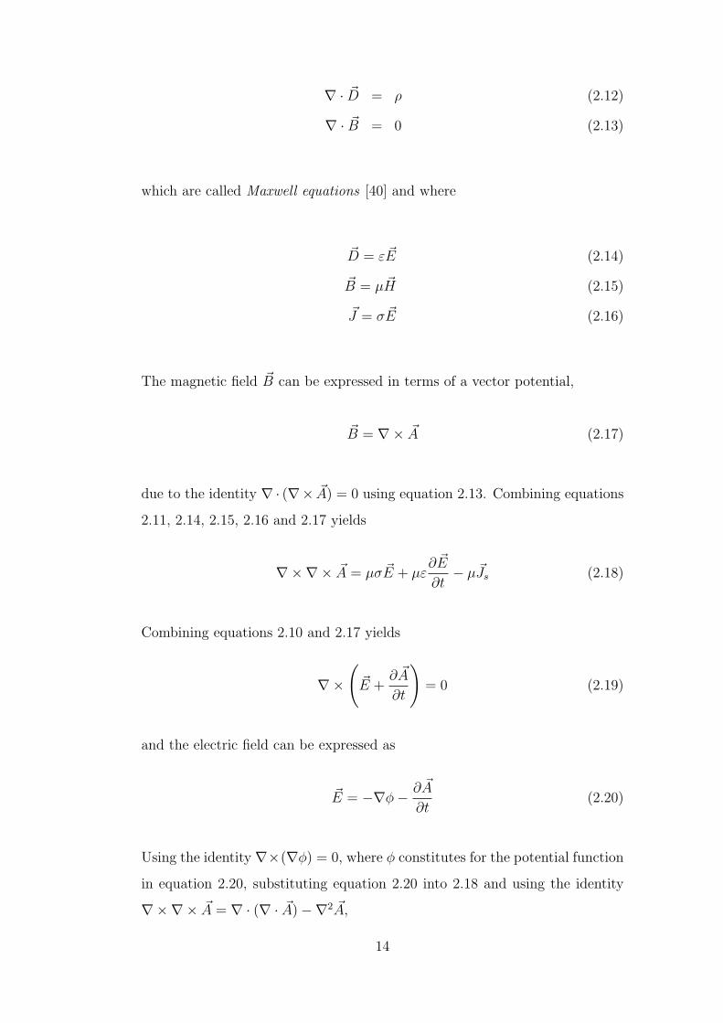
∇ · ~D = ρ (2.12)

∇ · ~B = 0 (2.13)

which are called Maxwell equations [40] and where

~D = ε ~E (2.14)

~B = µ ~H (2.15)

~J = σ ~E (2.16)

The magnetic field ~B can be expressed in terms of a vector potential,

~B = ∇× ~A (2.17)

due to the identity ∇ · (∇× ~A) = 0 using equation 2.13. Combining equations

2.11, 2.14, 2.15, 2.16 and 2.17 yields

∇×∇× ~A = µσ ~E + µε∂ ~E

∂t− µ~Js (2.18)

Combining equations 2.10 and 2.17 yields

∇×(

~E +∂ ~A

∂t

)= 0 (2.19)

and the electric field can be expressed as

~E = −∇φ− ∂ ~A

∂t(2.20)

Using the identity ∇×(∇φ) = 0, where φ constitutes for the potential function

in equation 2.20, substituting equation 2.20 into 2.18 and using the identity

∇×∇× ~A = ∇ · (∇ · ~A)−∇2 ~A,

14

∇ ·(∇ · ~A

)−∇2 ~A = ∇

[−

(µσφ + µε

∂φ

∂t

)]− µσ

∂ ~A

∂t− µε

∂2 ~A

∂t2(2.21)

If we choose Lorenz gauge valid for uniform medium

∇ · ~A = −(

µσφ + µε∂φ

∂t

)(2.22)

equation 2.21 takes the form

∇2 ~A− µσ∂ ~A

∂t− µε

∂2 ~A

∂t2= −µ ~Js (2.23)

where ~Js is the source current. If ~A has exponential characteristics (ejwt),

equation 2.23 can be expressed as,

∇2 ~A + k2 ~A = −µ ~Js (2.24)

where k2 = −jwµ (σ + jwε). Any vector field ~A generated by a volume current

~Js through the vector Helmholtz equation 2.24 has a solution for uniform,

unbounded medium:

~A(r) =

∫

V

~Js(r′)

e−jk|r−r′|

4πµ |r − r′|dr′ (2.25)

where r is the field point vector and r’ is the source point vector.

2.3 Combining MoM and Maxwell Relations

Four different geometries are considered for the source surface on which the

RF coil pattern is planned to be designed. For all of the considerations, MoM

is used to obtain the current density on the considered geometric surface and

the coil pattern is formed utilizing stream functions [41].

15

Maxwell Equations form the basis for the implementation of MoM. In or-

der to use MoM in the problem, magnetic flux density is expressed in terms

of current density by substituting 2.25 into 2.17. An integral equation in the

form of Fredholm Integral Equations

∫

Ω

K(x, x′)f(x

′)dx

′= g(x), x ∈ Ω (2.26)

is obtained. For this expression, which is stated in only one direction, x, for

the sake of simplicity

f (.) is the unknown function, which corresponds to the current density for

the described problem.

K (. , .) is the Kernel of the integral equation, which corresponds to the

relation between source and field points.

g (.) is the known or given function which is the magnetic flux density ~B for

the described problem.

In order to convert the integral equation into a matrix equation, f(x′) is ap-

proximated using basis functions such that

f(x′) ∼=N∑

j=1

αjfj(x′) (2.27)

where fj(x′) is the basis function for source point x′ and αj is the coefficient of

the basis function fj(x′) . In equation 2.27, f(x′) only depends on the coordi-

nate x′ ; however, for the defined problem, f(x′) ; in other words, the current

density is a function of x′ , y′ , z′ . The choice of the basis and weight functions

is explained in the Chapter 3.

When equation 2.27 is substituted into 2.26 the equality takes the form

16

N∑1

αj

∫

Ωj

f(x′j)K(xi, x

′j) dx

′= g(xi) (2.28)

Equation 2.6 can be expressed as a matrix equation in the form,

Ax = b (2.29)

where

x =

α1

α2

.

.

αN

N×1

(2.30)

b =

g(x1)

g(x2)

.

.

g(xM−1)

g(xM)

M×1

(2.31)

A =

f(x′1)K(x1, x

′1)dx′ f(x

′2)K(x1, x

′2)dx′ · · · f(x

′N)K(x1, x

′N)dx′

f(x′1)K(x2, x

′1)dx′ f(x

′2)K(x2, x

′2)dx′ · · · f(x

′N)K(x2, x

′N)dx′

.... . .

f(x′1)K(xM , x

′1)dx′ · · · f(x

′N)K(xM , x

′N)dx′

M×N

(2.32)

where N and M are the number of source and field points respectively.

17

2.4 Regularization

In a wide sense, inverse problems are concerned with the task of finding the

cause, given the effect.

A generic example of the inverse problem is the following: Let A : M → N

be a mapping between the sets, and suppose b ∈ N . The problem is then to

find x ∈ M such that Ax = b , or if no such x exists, such that Ax − b is

“small” in some sense.

A problem is referred to as ill–posed, in the sense that one or more of the

following conditions are violated:

1. There exists some solution x (existence)

2. There is only one solution (uniqueness)

3. The solution depends continuously on the data y (stability)

On the other hand, if all three conditions hold for a particular inverse problem,

the problem is referred to as well-posed. Fredholm Integral equations of the

first kind (of type I) which take the following form for functions defined in the

interval [0, 1]:

∫ 1

0

k(s, t)x(t) dt = y(s) , 0 ≤ s ≤ 1 (2.33)

are usually ill-posed problems [42].

A function f : G → H mapping elements in a linear space (a vector space) G

into a linear space H is called linear if we have f(αx + βy) = α f(x) + β f(y)

for all x, y ∈ G and α, β ∈ R . Let G and H be Euclidean spaces, such

that f : Rm → Rn for some integers m, n > 0 . Then there exists a matrix

A ∈ Rm,n such that f(x) = Ax for all x ∈ Rn . Suppose we have the linear

rather relationship Ax = b between the vectors b ∈ Rm and x ∈ Rn where

18

x might represent parameters of a physical system or the input to the system,

A is the transformation performed by the system on the input and b is the

output from the system.

The problem of computing b when A and x are given, is an example of a

forward problem which obviously has only one solution. Since the relationship

between x and b is linear, the right hand side b is a continuous function of x.

Thus, the solution is stable in the sense that small changes in x will result in

small changes in b . Theoretically, this problem is therefore well-posed. If A

is ill-conditioned, the direct problem may still be ill-posed in a weaker sense.

In this case, regularization may be applied.

Suppose A and b are known and x is to be determined. Here, x is only

implicitly given by the equation Ax = b , hence this is an inverse problem.

Existence and uniqueness of the solution is only guaranteed under certain as-

sumptions. The simplest case arises when rank(A) = p = n and therefore A is

invertible. The inverse problem is then obviously also well-posed in theory. If

A is not invertible, we see that a solution exists if and only if b is an element of

the range space, b ∈ <(A) and the solution is unique if and only if null space

of A is an empty set, N(A) = 0 . Furthermore, when a unique solution

exists it is only stable if <(A) = Rn (implying that A is invertible) [42].

There are three possible scenarios [43]:

1. The system is full rank; i.e., the number of equations equals the number

of unknowns. In this case, there is only one solution which is given by

x = A−1b (2.34)

2. The matrix A has more rows than columns; i.e., there are more equations

than unknowns. An exact solution for the system does not exist, so this

problem is solved in the mean square sense. The solution is chosen to be the

19

vector x that satisfies the least squares equation

x = arg minx

‖b−Ax ‖22 (2.35)

Recall that x is a least squares solution if and only if the normal equations

AT (b−Ax) = 0 (2.36)

are satisfied. This means that the error (b−Ax) in the approximation is

in the subspace N(AT

). Geometrically, the least squares solution x is the

orthogonal projection of b into < (A). Provided N(A) = 0 there is a unique

least squares solution given by

x = (ATA)−1ATb (2.37)

3. The matrix A has more columns than rows; i.e., there are more unknowns

than equations. There are infinitely many solutions for this type of system,

which is also solved in a mean square sense. The solution x is chosen to be

the minimum energy solution to the least squares equation, which is also the

solution to cases 2.33 and 2.34 and is given by

x = arg minx

‖x‖22 subject to min ‖b−Ax‖2

2 (2.38)

The superior numerical tools for analysis of rank-deficient and discrete ill-posed

problems are Singular Value Decomposition (SVD) of A and its generalization

to two matrices, the generalized SVD (GSVD) of the matrix pair (A,L) . The

SVD reveals all the difficulties associated with the ill-conditioning of the matrix

A , while GSVD of (A,L) yields important insight into the regularization

problems involving both the matrix A and the regularization matrix L .

20

2.4.1 The Idea of Regularization

Most regularization methods produce an estimate of the form

x = VFD−1UTb =n∑

i=1

fi〈ui, b〉

σi

vi (2.39)

The matrices V, D, U are the matrices obtained by the SVD of A . There is an

additional scale factor fi for each term in the sum. These factors usually sat-

isfy 0 ≤ fi ≤ 1 , corresponding to the notion that regularization down weights

or filters out some of the directions vi , usually those that are associated with

smaller singular values σi . The diagonal matrix F which is composed of the

diagonal elements f1, f2, . . . fn , completely characterizes the filtering proper-

ties of the regularization method. The matrix A# = VFD−1UT is called the

regularization matrix, as we have x = A#b [42].

2.5 Stream Functions

The definition of a streamline is the line everywhere tangential to the local

fluid velocity, i.e., the solution of

dx

u=

dy

v=

dz

w(2.40)

where u, v and w are the speeds of the fluid in x, y and z directions respec-

tively. It has been shown that, in order to construct accurate streamlines,

mass conservation must be maintained. This means that the divergence of the

fluid momentum must be zero [44]

∇ · (ρ~F ) = 0 (2.41)

where ρ is the fluid density and ~F is the fluid velocity.

21

The stream function was first introduced by Lagrenge to describe two-dimensional

incompressible flow (∇· ~F = 0). This condition allows ~F to be described as the

curl of a vector potential with a single component ψ in perpendicular direction

to the surface where ~F is defined [41]. The function ψ is the stream function,

and it is related to vector field through the equation

~F = ∇× ψ~n (2.42)

where ~n is the unit vector perpendicular to the surface on which ~F is defined.

Equation 2.42 yields the following relation for cartesian coordinates between

the stream function and vector field which has two normal components u~ax

and u~ay on xy-plane:

u =∂ψ

∂y

v =−∂ψ

∂x(2.43)

It can be seen that 2.43 can be arranged to obtain

udy − vdx = 0 (2.44)

so that

dψ = 0 (2.45)

and ψ is constant along the streamline. This is an important result as it means

that a streamline can be formed by computing contours of the scalar field ψ

[45].

22

The stream function also has an important physical property which is related

to the mass flow rate between two points in the flow field. Let us consider the

vector field as an divergence free surface current density ~Js on an arbitrary

surface Ω. From the definition of the current density [40], the total current

flowing through an arbitrary surface Ω is

I =

∫

Ω

~J · ~ds (2.46)

When dealing with the sheet current density ~Js, 2.46 can be modified to

I =

∫

`

~Js · ~dl (2.47)

Figure 2.1: Equally spaced contours of ψ represent winding patterns withconstant current in each streamline. The difference between the magnitude ofψ2 at point (x2, y2) and the magnitude of ψ1 at point (x1, y1) is equal to themagnitude of the current I12 flowing between the streamlines ψ1 and ψ2.

With the line integral split into smaller segments, the change in current

across a segment is

23

I12 =

∫ l2

l1

~Js · ~ndl (2.48)

=

∫ l2

l1

uδy − vδx (2.49)

=

∫ l2

l1

dψ = ψ2 − ψ1 (2.50)

This shows that a spatial change in the value of ψ corresponds to an equivalent

change in the value of the current I and that contour plots of ψ(x, y) will give

the locations of discrete wires carrying equal currents.

It can be shown that streamlines, lines where ψ = constant, are everywhere

parallel to the current sheet density vector ~Js = Jx~ax + Jy~ay. For ∇ · ~Js = 0

~Js =∂ψ

∂y~ax − ∂ψ

∂x~ay (2.51)

Any point on the curve ψ = constant can be expressed in cartesian coordinates

as

~r = x(s)~ax − y(s)~ay (2.52)

where s is the arc length along the streamline curve. The unit vector to this

streamline is

~T =d~r

ds=

dx

ds~ax +

dy

ds~ay (2.53)

For the streamline ψ(x(s), y(s)) = constant, the chain rule yields

dψ

ds=

∂ψ

∂x

dx

ds+

∂ψ

∂y

dy

ds(2.54)

Using 2.51,

24

dy

ds=

Jy

Jx

dx

ds(2.55)

Substituting 2.51 into, 2.53 gives the result:

~T =1

Jx

dx

ds(Jx~ax + Jy~ay) (2.56)

which means that current flow is parallel to the streamlines.

25

CHAPTER 3

Implementing the Coil Structure by Using

Regularization Methods and Stream Functions

3.1 Defining the Required Magnetic Field

The main purpose of the algorithm defined in this report is to find a current

density map on a pre-defined surface in order to create a specified magnetic

field within a predefined volume. Therefore, magnetic field specification is one

of the inputs that should be defined. As the aim of this work is to produce a

coil that generates an RF field for an inhomogeneous main field, the charac-

teristics of the RF field should also be determined with reference to the main

magnetic field. In order to specify an RF field, first an inhomogeneous mag-

netic field is produced by a square coil placed on the yz − plane, within the

pre-defined field volume as illustrated in 3.1 and for each field point, RF field

components are specified based on the requirements related to this main field.

The main magnetic field in the target volume that is considered as a reference

to produce RF field is illustrated in Figure 3.1.

The first requirement on the RF field is that, the field produced by the coil

should be perpendicular to the main magnetic field at every field point. In

other words, if a single field point and the main field vector at this point are

considered, then the RF field vector is defined on the plane which the main

field vector is normal to.

26

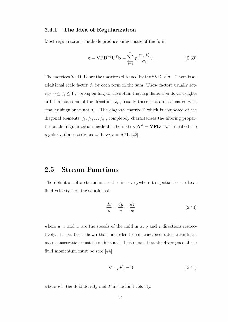
For this requirement to be satisfied, the main magnetic field and the RF field

are defined as:

Figure 3.1: Main magnetic field Vectors in the field volume. A square wire of10cm by 10cm is considered on yz-plane. The center of the square coil is atpoint (0,0,0) and the coil generates magnetic field vectors represented by thearrows of length proportional to the magnitudes at every field point.

~B = Bx~ax + By~ay + Bz~az

~Brf = Brx~ax + Bry~ay + Brz~az

(3.1)

Then, the orthogonality principle, which is a preferred constraint for RF field

determination, requires that

~B · ~Brf = 0 (3.2)

which results in the equality

27

BxBrx(t) + ByBry(t) + BzBrz(t) = 0 (3.3)

A second preferred constraint on the RF field is that, at every field point the

magnitude of the field vector should be equal so that the spins at every field

point is forced onto the transverse plane of the field vector at the same time.

For this requirement to be satisfied:

√B2

rx + B2ry + B2

rz = m (3.4)

where m is a non-zero real number.

In order to determine an RF field as the desired magnetic field, four different

magnetic field characteristics are considered specifying different requirements.

3.1.1 RF Field Case 1

For these characteristics, only the first requirement is considered and the x

and y components of the RF field are specified as:

Brx = Bx and Bry = By (3.5)

From equation 3.3 it is determined that

Brz = −B2x + B2

y

Bz

(3.6)

Using the main magnetic field B and the equations 3.5, 3.6, one of the possible

RF field characteristics is determined as illustrated in Figure 3.2.

28

Figure 3.2: Main magnetic field and RF field vectors within the field volumefor case 1. The main magnetic field vectors are illustrated as blue arrows,while RF field vectors are illustrated as red arrows.


For this characteristics, both requirements are considered and y component of

the RF field is specified as zero at all field points, so that the spin interactions

are decreased as all spins will lie perpendicular to the y-axis when RF field is

applied. Therefore, equation 3.4 takes the form:

B2rx + B2

rz = m2 (3.7)

From 3.3,

Brx =−BrzBz

Bx

(3.8)

If 3.8 is substituted in 3.7, it is found that

29

Brz =|mBx|√B2

x + B2z

(3.9)

From 3.9,

Brx = −|mBx|Bx

· Bz√B2

x + B2z

(3.10)

And it is initially defined that

Bry = 0 (3.11)

Using the main magnetic field B and the equations 3.9, 3.10, 3.11; another

possible RF field characteristics is determined as illustrated in Figure 3.3.


30


For this characteristics, both requirements are considered. Also it is specified

that the component of the RF field on the xy-plane is in the same or opposite

direction as the one of the main magnetic field. This requires:

Brx

Bry

=Bx

By

(3.12)

Using equations 3.3 and 3.4,

Bry = ∓√√√√ m2

B2x+B2

y

B2y

+(B2

x+B2y)

2

B2yB2

z

(3.13)

where the minus or plus sign determines whether the transverse components

of the fields are in the same or opposite direction respectively.

Brx =Bx

By

Bry (3.14)

and

Brz = −B2x + B2

y

ByBz

Bry (3.15)

Using the main magnetic field B and the equations 3.13, 3.14, 3.15 ; another



For this characteristics, both requirements are considered and it is specified

that the y-component of the RF field is constant at all field points, so that it

could be tested whether the regularization works better for such characteristics

that is forced to be more homogeneous. For a constant y-component,

Bry = a (3.16)

31


where a is a positive real number. Combining 3.4 and 3.16,

B2rx = m2 − a2 −B2

rz (3.17)

and combining 3.3 and 3.17,

Brz =−2aByBz ∓

√4a2B2

yB2z − 4 (B2

x + B2z )

(a2B2

y + a2B2x −m2B2

x

)

2 (B2x + B2

z )(3.18)

And using 3.3,

Brx = −mBy + BzBrz

Bx

(3.19)

32

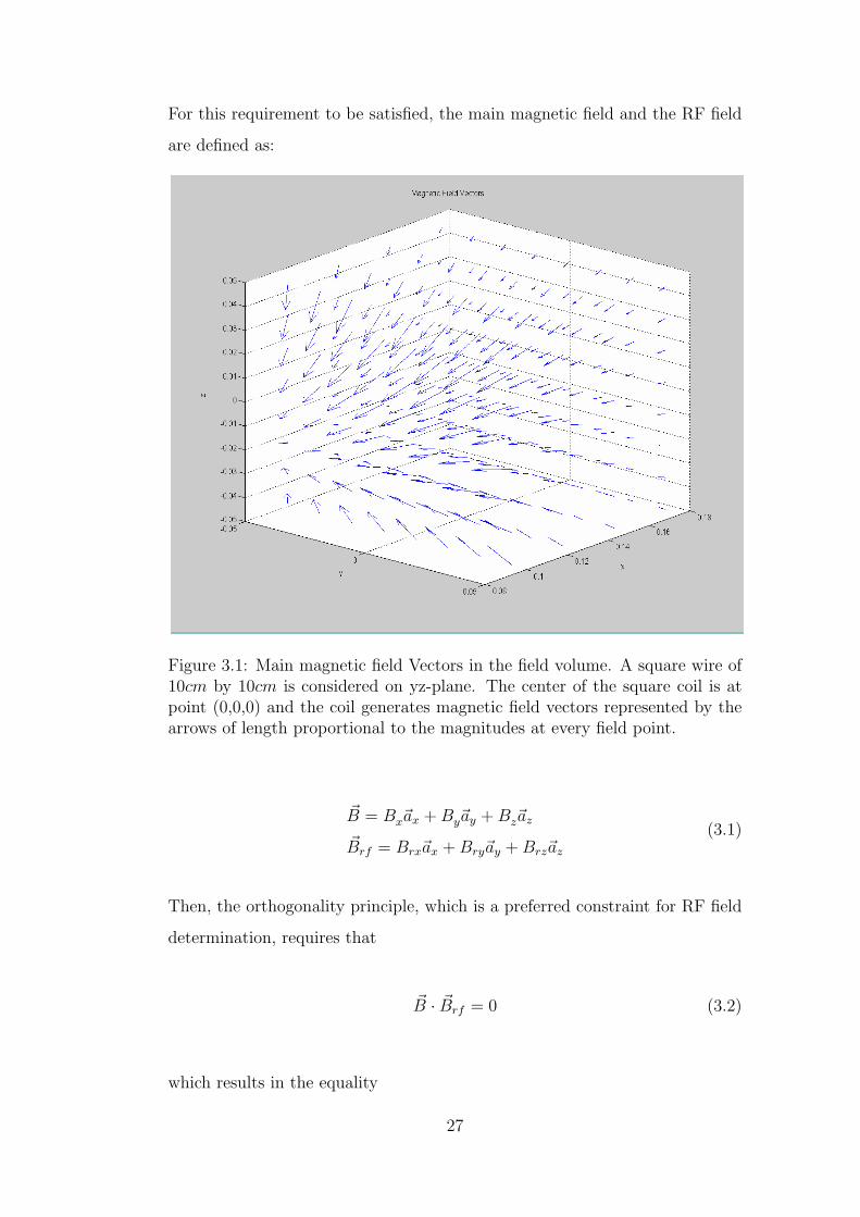
Using the main magnetic field B and the equations 3.16, 3.18, 3.19; another


Figure 3.5: Main magnetic field and RF field vectors within the field volumefor case 4. The main magnetic field vectors are illustrated as blue arrows, whileRF field vectors are illustrated as red arrows. RF Field vector magnitudes arescaled by a factor of 0.5.

3.2 Defining Target and Source Fields

Four different geometries are considered as source fields where surface current

density is defined. Target fields are defined as cubes with their centers placed at

the origin. The problem definitions are named after the source field geometries

on which the surface current density vectors are defined:

• Cylindrical Surface,

• Planar Surface,

33

• Tri-planar Surface and

• Orthogonal Three Planes

3.2.1 Cylindrical Source Surface

The required RF field is aimed to be generated within the cube at the origin by

the surface current density vectors in angular and vertical directions defined

on a cylinder of radius ρ0 and length L which surrounds the target field. The

source and target fields for this problem definition are illustrated in Figure 3.6.

Figure 3.6: Target and source fields for cylindrical surface problem defini-tion.The cube inside the cylinder is the target field while the cylindrical surfaceis the source field.

In order to carry out the MoM solution, the surface of the cylinder is divided

into M longitudinal and N angular pieces forming M × N subdomains. The

mapping of cylinder surface into two dimensional grid structure is illustrated

in Figure 3.7.

34

Figure 3.7: Spatial mapping of cylinder surface coordinates onto subdomains.

3.2.2 Tri-Planar Source Surface

The required RF field is aimed to be generated within the cube at the origin

by the surface current density vectors on a geometry formed by three planes,

one of which is placed parallel to yz − plane and the remaining two parallel

to each other and xz − plane. This surface geometry has a total longitudinal

length of L and a width of W . The source and target fields for this problem

definition are illustrated in Figure 3.8.

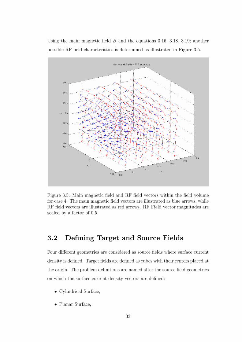
35

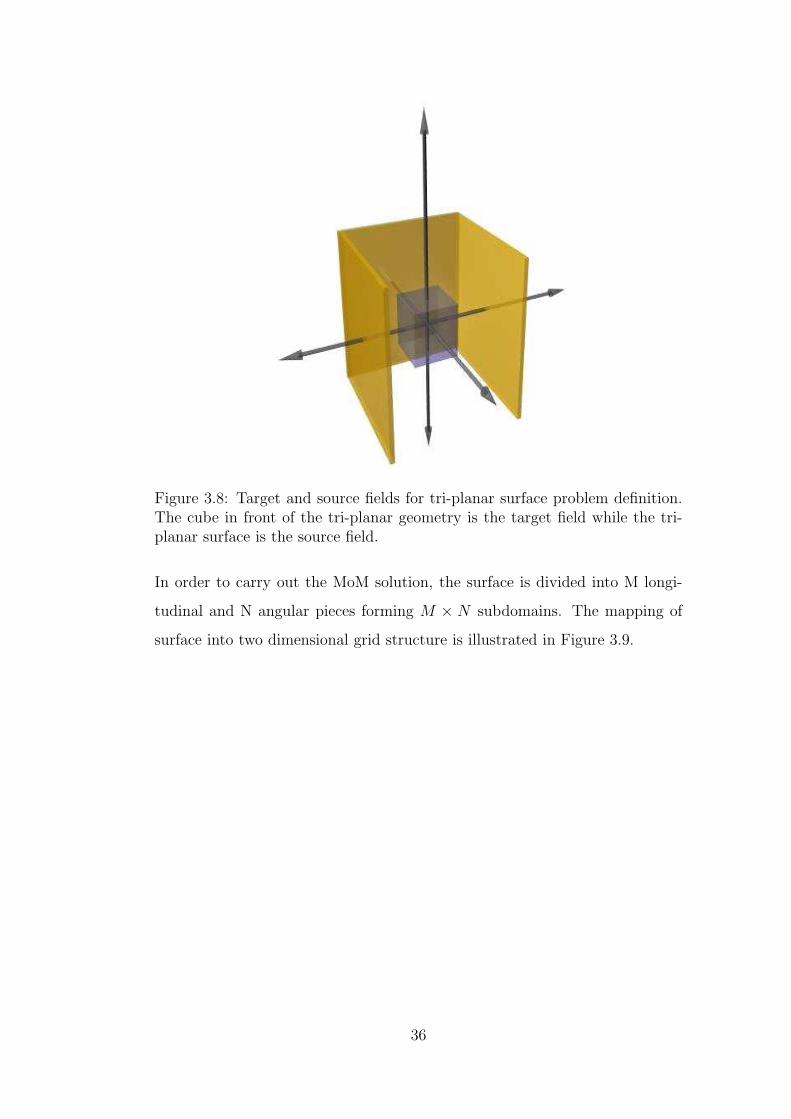
Figure 3.8: Target and source fields for tri-planar surface problem definition.The cube in front of the tri-planar geometry is the target field while the tri-planar surface is the source field.

In order to carry out the MoM solution, the surface is divided into M longi-

tudinal and N angular pieces forming M × N subdomains. The mapping of

surface into two dimensional grid structure is illustrated in Figure 3.9.

36

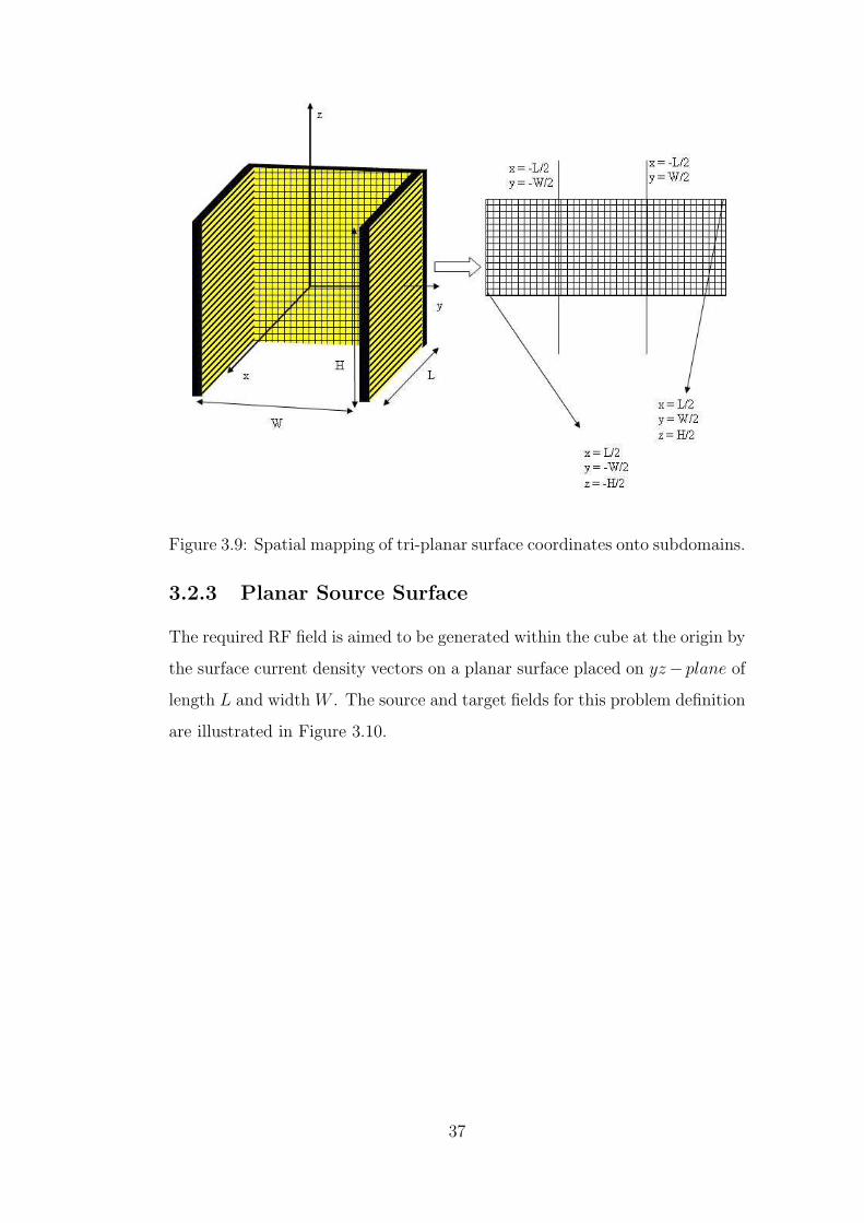
Figure 3.9: Spatial mapping of tri-planar surface coordinates onto subdomains.

3.2.3 Planar Source Surface


the surface current density vectors on a planar surface placed on yz− plane of

length L and width W . The source and target fields for this problem definition

are illustrated in Figure 3.10.

37

Figure 3.10: Target and source fields for planar surface problem definition.Thecube in front of the planar geometry is the target field while the planar surfaceis the source field.

In order to carry out the MoM solution, the planar surface is divided into M

pieces on z − axis and N pieces on y − axis forming M ×Nsubdomains.

3.2.4 Orthogonal Three Planes


the surface current density vectors on a geometry formed by three planes, that

are placed on three different planes orthogonal to each other. As a definition

of this problem, each plane acts as an independent planar surface that aims to

generate one directional component of the required RF field, which is directed

normal to the corresponding plane. Each planar surface geometry has a length

and width equal to each other. The source and target fields for this problem

definition are illustrated in Figure 3.11.

38

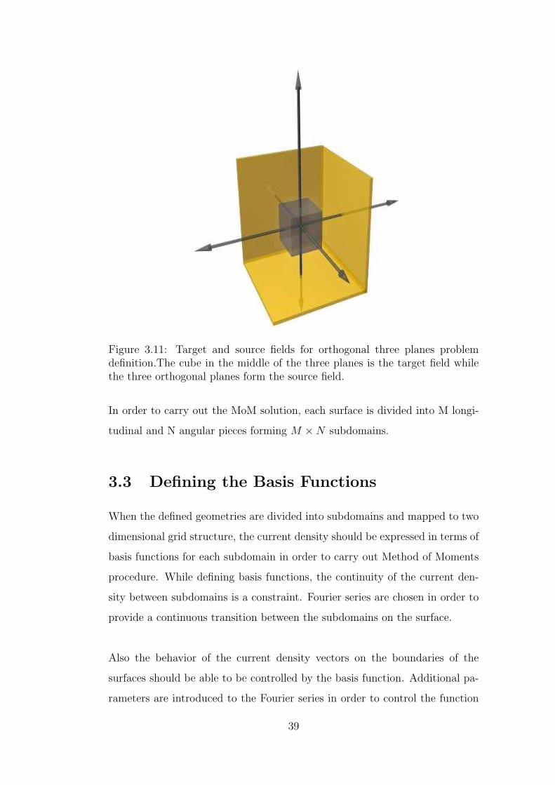
Figure 3.11: Target and source fields for orthogonal three planes problemdefinition.The cube in the middle of the three planes is the target field whilethe three orthogonal planes form the source field.

In order to carry out the MoM solution, each surface is divided into M longi-

tudinal and N angular pieces forming M ×N subdomains.

3.3 Defining the Basis Functions

When the defined geometries are divided into subdomains and mapped to two

dimensional grid structure, the current density should be expressed in terms of

basis functions for each subdomain in order to carry out Method of Moments

procedure. While defining basis functions, the continuity of the current den-

sity between subdomains is a constraint. Fourier series are chosen in order to

provide a continuous transition between the subdomains on the surface.

Also the behavior of the current density vectors on the boundaries of the

surfaces should be able to be controlled by the basis function. Additional pa-

rameters are introduced to the Fourier series in order to control the function

39

magnitude on the surface boundaries.

Two general basis function sets are defined for the current density vectors.

The first definition is used for the cylindrical geometry while the second defi-

nition is used for planar geometries.

3.3.1 Basis Functions for Cylindrical Geometry

The basis functions used for current densities in angular and longitudinal di-

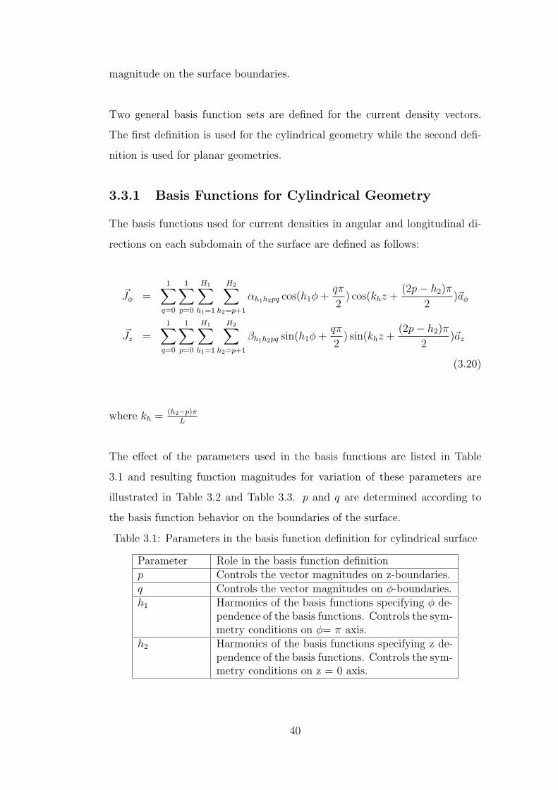
rections on each subdomain of the surface are defined as follows:

~Jφ =1∑

q=0

1∑p=0

H1∑

h1=1

H2∑

h2=p+1

αh1h2pq cos(h1φ +qπ

2) cos(khz +

(2p− h2)π

2)~aφ

~Jz =1∑

q=0

1∑p=0

H1∑

h1=1

H2∑

h2=p+1

βh1h2pq sin(h1φ +qπ

2) sin(khz +

(2p− h2)π

2)~az

(3.20)

where kh = (h2−p)πL

The effect of the parameters used in the basis functions are listed in Table

3.1 and resulting function magnitudes for variation of these parameters are

illustrated in Table 3.2 and Table 3.3. p and q are determined according to

the basis function behavior on the boundaries of the surface.

Table 3.1: Parameters in the basis function definition for cylindrical surface

Parameter Role in the basis function definitionp Controls the vector magnitudes on z-boundaries.q Controls the vector magnitudes on φ-boundaries.h1 Harmonics of the basis functions specifying φ de-

pendence of the basis functions. Controls the sym-metry conditions on φ= π axis.

h2 Harmonics of the basis functions specifying z de-pendence of the basis functions. Controls the sym-metry conditions on z = 0 axis.

40

Table 3.2: Basis function characteristics for Cylindrical Surface varying p, q,H1 and H2 - 1

p=0, q=0 p=0, q=1Jφ Jz Jφ Jz

H1=1H2=1

H1=2H2=2

H1=3H2=3

H1=4H2=4

41

Table 3.3: Basis function characteristics for Cylindrical Surface varying p, q,H1 and H2 - 2

p=1, q=0 p=1, q=1Jφ Jz Jφ Jz

H1=2H2=2

H1=3H2=3

H1=4H2=4

3.3.1.1 Stream Functions

The az and aφ sinusoidal terms spatially differ by 900 because this form gives

a convenient description of the scalar functions and that fully describe the

current density as a sum of a rotational (R) and irrotational (I) term:

~J = ~Jφ + ~Jz = ~JR + ~JI (3.21)

or in terms of scalar functions ψ and χ

~J = ~aρ ×∇χ +∇Ψ (3.22)

such that

ψ =1∑

q=0

1∑p=0

H1∑

h1=1

H2∑

h2=p+1

γh1h2pq sin( h1φ +qπ

2) cos( khz +

(2p− h2)π

2)

42

χ =1∑

q=0

1∑p=0

H1∑

h1=1

H2∑

h2=p+1

κh1h2pq cos(h1φ +qπ

2) sin(khz +

(2p− h2)π

2)

(3.23)

where ∇ = ∂∂φ

~aφ + ∂∂z

~az

If the coil structure is very small relative to the wavelength of operation, the

current density ~J is purely rotational [33]. This situation is valid for low

operating frequencies such as METU MRI system (6.387 MHz). Therefore,

the current density is approximated without divergence. As current density

function is purely rotational

γh1h2pq = 0 and βh1h2pq =h1αh1h2pq

ρ0kh

(3.24)

Therefore, current density functions can be rewritten as:

~Jφ =

H1∑

h1=1

H2∑

h2=1

αh1h2 cos(h1φ) cos(khz − h2π

2)~aφ

~Jz =

H1∑

h1=1

H2∑

h2=1

h1αh1h2

ρ0kh

sin(h1φ) sin(khz − h2π

2)~az

ψ =

H1∑

h1=1

H2∑

h2=1

−αh1h2pq

kh

sin( h1φ ) cos( khz − h2π

2)

(3.25)

where kh = h2πL

, (p = 0, q = 0)

3.3.2 Basis Functions for Planar Geometries

A general form of Fourier series is used for planar geometries. The basis

functions used for current densities on each subdomain of the surface are as

follows:

43

~Ju =1∑

q=0

1∑p=0

H1∑

h1=1

H2∑

h2=1

αh1h2pq cos(kh1u +qπ

2) cos(kh2v +

pπ

2)~au

~Jv =1∑

q=0

1∑p=0

H1∑

h1=1

H2∑

h2=1

βh1h2pq sin(kh1u +qπ

2) sin(kh2v +

pπ

2)~av

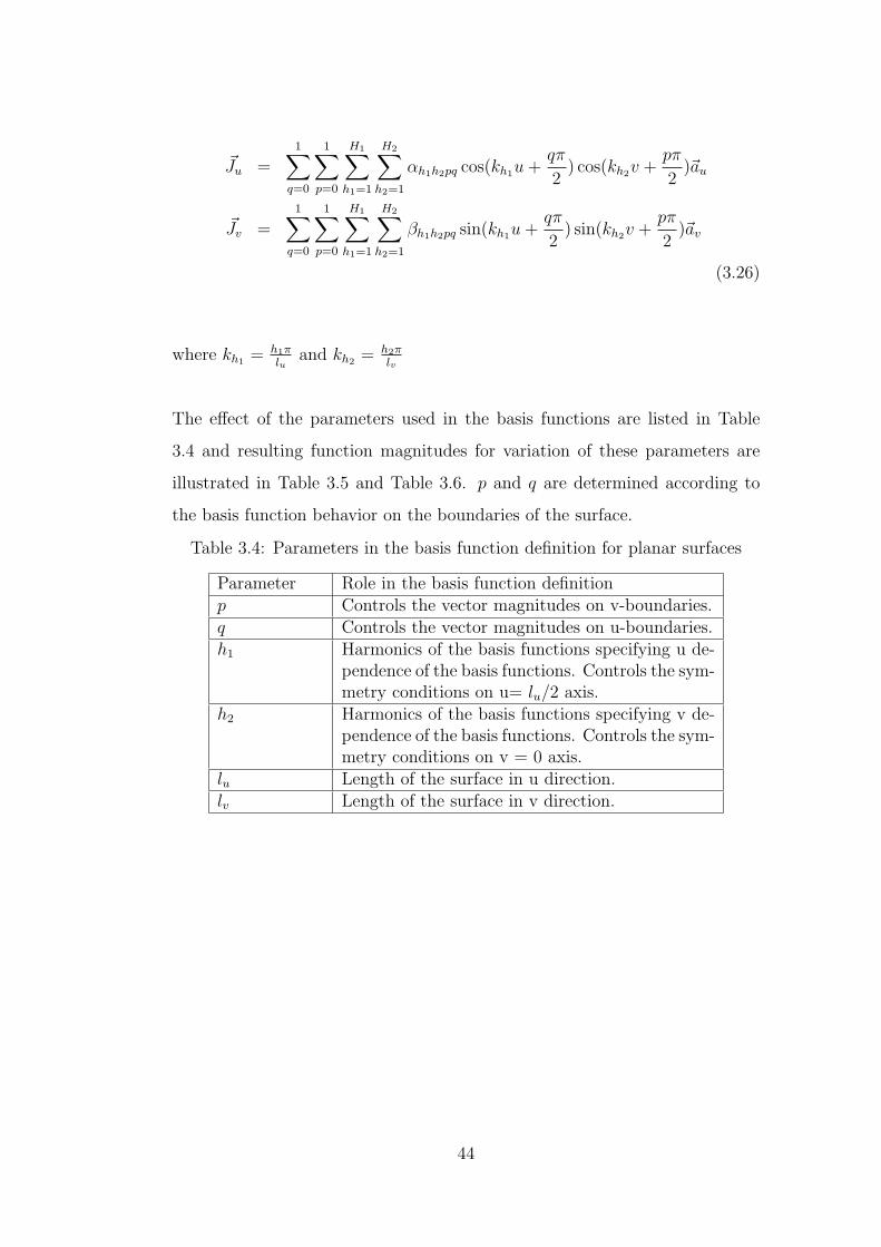
(3.26)

where kh1 = h1πlu

and kh2 = h2πlv

The effect of the parameters used in the basis functions are listed in Table

3.4 and resulting function magnitudes for variation of these parameters are

illustrated in Table 3.5 and Table 3.6. p and q are determined according to

the basis function behavior on the boundaries of the surface.

Table 3.4: Parameters in the basis function definition for planar surfaces

Parameter Role in the basis function definitionp Controls the vector magnitudes on v-boundaries.q Controls the vector magnitudes on u-boundaries.h1 Harmonics of the basis functions specifying u de-

pendence of the basis functions. Controls the sym-metry conditions on u= lu/2 axis.

h2 Harmonics of the basis functions specifying v de-pendence of the basis functions. Controls the sym-metry conditions on v = 0 axis.

lu Length of the surface in u direction.lv Length of the surface in v direction.

44

Table 3.5: Basis function characteristics for planar geometries varying p, q, H1

and H2 - 1

p=0, q=0 p=0, q=1Ju Jv Ju Jv

H1=1H2=1

H1=2H2=2

H1=3H2=3

H1=4H2=4

45

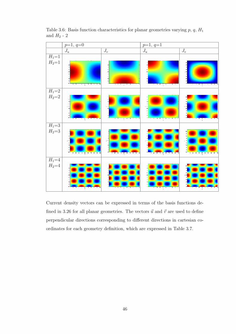
Table 3.6: Basis function characteristics for planar geometries varying p, q, H1

and H2 - 2

p=1, q=0 p=1, q=1Ju Jv Ju Jv

H1=1H2=1

H1=2H2=2

H1=3H2=3

H1=4H2=4

Current density vectors can be expressed in terms of the basis functions de-

fined in 3.26 for all planar geometries. The vectors ~u and ~v are used to define

perpendicular directions corresponding to different directions in cartesian co-

ordinates for each geometry definition, which are expressed in Table 3.7.

46

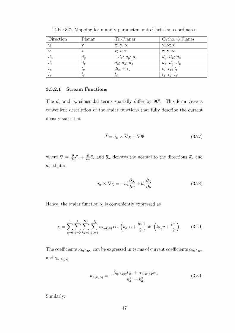
Table 3.7: Mapping for u and v parameters onto Cartesian coordinates

Direction Planar Tri-Planar Ortho. 3 Planesu y x; y; x y; x; zv z z; z; z z; y; x~au ~ay −~ax; ~ay; ~ax ~ay; ~ax; ~az

~av ~az ~az; ~az; ~az ~az; ~ay; ~ax

lu ly 2lx + ly ly; lx; lzlv lz lz lz; ly; lx

3.3.2.1 Stream Functions

The ~au and ~av sinusoidal terms spatially differ by 900. This form gives a

convenient description of the scalar functions that fully describe the current

density such that

~J = ~aw ×∇χ +∇Ψ (3.27)

where ∇ = ∂∂u

~au + ∂∂v

~av and ~aw denotes the normal to the directions ~au and

~av; that is

~aw ×∇χ = − ~au∂χ

∂v+ ~av

∂χ

∂u(3.28)

Hence, the scalar function χ is conveniently expressed as

χ =1∑

q=0

1∑p=0

H1∑

h1=1

H2∑

h2=1

κh1h2pq cos(kh1u +

qπ

2

)sin

(kh2v +

pπ

2

)(3.29)

The coefficients κh1h2pq can be expressed in terms of current coefficients αh1h2pq

and γh1h2pq

κh1h2pq = −βh1h2pqkh1 + αh1h2pqkh1

k2h1

+ k2h2

(3.30)

Similarly:

47

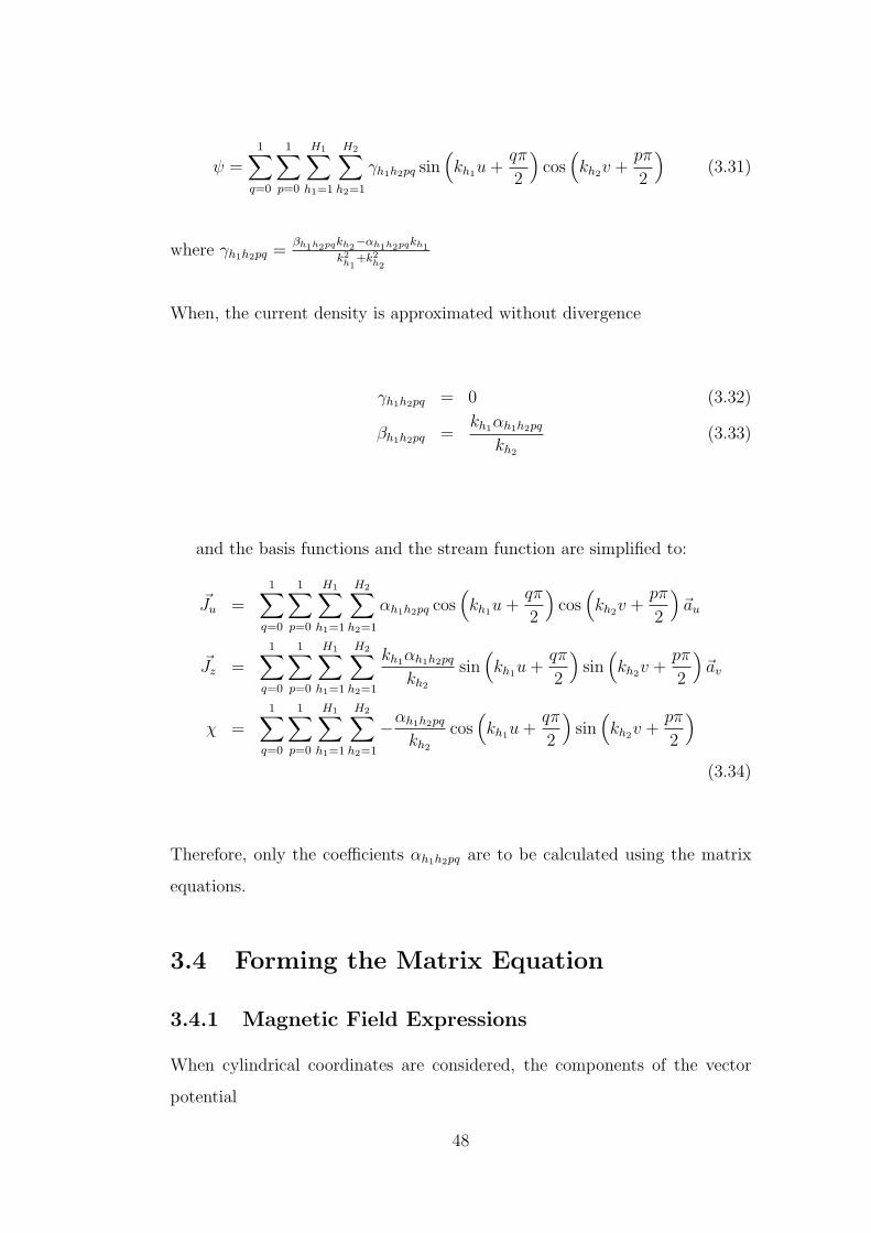
ψ =1∑

q=0

1∑p=0

H1∑

h1=1

H2∑

h2=1

γh1h2pq sin(kh1u +

qπ

2

)cos

(kh2v +

pπ

2

)(3.31)

where γh1h2pq =βh1h2pqkh2

−αh1h2pqkh1

k2h1

+k2h2

When, the current density is approximated without divergence

γh1h2pq = 0 (3.32)

βh1h2pq =kh1αh1h2pq

kh2

(3.33)

and the basis functions and the stream function are simplified to:

~Ju =1∑

q=0

1∑p=0

H1∑

h1=1

H2∑

h2=1

αh1h2pq cos(kh1u +

qπ

2

)cos

(kh2v +

pπ

2

)~au

~Jz =1∑

q=0

1∑p=0

H1∑

h1=1

H2∑

h2=1

kh1αh1h2pq

kh2

sin(kh1u +

qπ

2

)sin

(kh2v +

pπ

2

)~av

χ =1∑

q=0

1∑p=0

H1∑

h1=1

H2∑

h2=1

−αh1h2pq

kh2

cos(kh1u +

qπ

2

)sin

(kh2v +

pπ

2

)

(3.34)

Therefore, only the coefficients αh1h2pq are to be calculated using the matrix

equations.

3.4 Forming the Matrix Equation

3.4.1 Magnetic Field Expressions

When cylindrical coordinates are considered, the components of the vector

potential

48

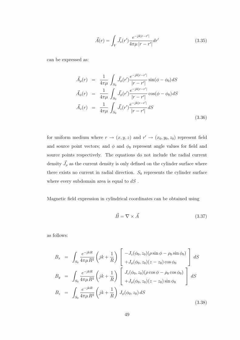
~A(r) =

∫

V

~Js(r′)

e−jk|r−r′|

4πµ |r − r′|dr′ (3.35)

can be expressed as:

~Aρ(r) =1

4πµ

∫

S0

~Jφ(r′)

e−jk|r−r′|

|r − r′| sin(φ− φ0)dS

~Aφ(r) =1

4πµ

∫

S0

~Jφ(r′)

e−jk|r−r′|

|r − r′| cos(φ− φ0)dS

~Az(r) =1

4πµ

∫

S0

~Jz(r′)

e−jk|r−r′|

|r − r′| dS

(3.36)

for uniform medium where r → (x, y, z) and r′ → (x0, y0, z0) represent field

and source point vectors; and φ and φ0 represent angle values for field and

source points respectively. The equations do not include the radial current

density ~Jρ as the current density is only defined on the cylinder surface where

there exists no current in radial direction. S0 represents the cylinder surface

where every subdomain area is equal to dS .

Magnetic field expression in cylindrical coordinates can be obtained using

~B = ∇× ~A (3.37)

as follows:

Bx =

∫

S0

e−jkR

4πµR2

(jk +

1

R

) −Jz(φ0, z0)(ρ sin φ− ρ0 sin φ0)

+Jφ(φ0, z0)(z − z0) cos φ0

dS

By =

∫

S0

e−jkR

4πµR2

(jk +

1

R

) Jz(φ0, z0)(ρ cos φ− ρ0 cos φ0)

+Jφ(φ0, z0)(z − z0) sin φ0

dS

Bz =

∫

S0

e−jkR

4πµR2

(jk +

1

R

)Jφ(φ0, z0) dS

(3.38)

49

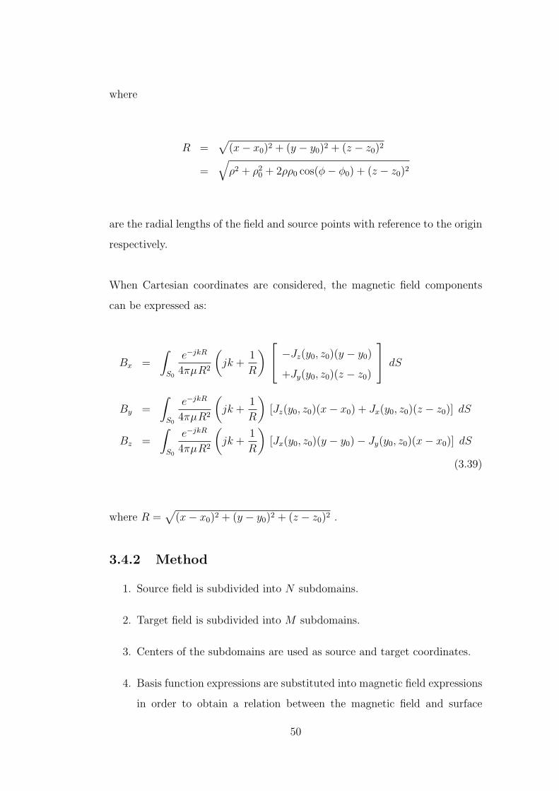
where

R =√

(x− x0)2 + (y − y0)2 + (z − z0)2

=√

ρ2 + ρ20 + 2ρρ0 cos(φ− φ0) + (z − z0)2

are the radial lengths of the field and source points with reference to the origin

respectively.

When Cartesian coordinates are considered, the magnetic field components

can be expressed as:

Bx =

∫

S0

e−jkR

4πµR2

(jk +

1

R

) −Jz(y0, z0)(y − y0)

+Jy(y0, z0)(z − z0)

dS

By =

∫

S0

e−jkR

4πµR2

(jk +

1

R

)[Jz(y0, z0)(x− x0) + Jx(y0, z0)(z − z0)] dS

Bz =

∫

S0

e−jkR

4πµR2

(jk +

1

R

)[Jx(y0, z0)(y − y0)− Jy(y0, z0)(x− x0)] dS

(3.39)

where R =√

(x− x0)2 + (y − y0)2 + (z − z0)2 .

3.4.2 Method

1. Source field is subdivided into N subdomains.

2. Target field is subdivided into M subdomains.

3. Centers of the subdomains are used as source and target coordinates.

4. Basis function expressions are substituted into magnetic field expressions

in order to obtain a relation between the magnetic field and surface

50

current density for ith target field and jth source field in the following

form:

Bx,i =N∑

j=1

H1∑

h1=1

H2∑

h2=1

αh1h2,jKxh1h2,ij

By,i =N∑

j=1

H1∑

h1=1

H2∑

h2=1

αh1h2,jKyh1h2,ij

Bz,i =N∑

j=1

H1∑

h1=1

H2∑

h2=1

αh1h2,jKzh1h2,ij

(3.40)

where i = 1, 2, . . .M and j = 1, 2, . . . N and for cylindrical source field

and for

G(R) =e−jkR

4πµR2

(jk +

1

R

)(3.41)

Kxh1h2,ij = G(R)

− kn

kmcos (kny0,j) cos (kmz0,j) (yi − y0,j)

+ sin (kny0,j) sin (kmz0,j) (zi − z0,j)

∆S

Kyh1h2,ij = G(R)

h1ρ0kh

sin(h1φ0,j) sin(khz0,j − h2π2 )(ρ cos φi − ρ0 cos φ0,j)

+ cos(h1φ0,j) cos(khz0,j − h2π2 )(zi − z0,j) sin φ0,j

∆S

Kzh1h2,ij = G(R) cos(h1φ0,j) cos(khz0,j − h2π

2)∆S

(3.42)

while for planar source field on yz-plane:

Kxh1h2,ij = G(R)

− kn

kmcos (kny0,j) cos (kmz0,j) (yi − y0,j)

+ sin (kny0,j) sin (kmz0,j) (zi − z0,j)

∆S

Kyh1h2,ij = G(R) [cos (kny0) cos (kmz0) (xi − x0,j)] ∆S

Kzh1h2,ij = G(R) [− sin (kny0,j) sin (kmz0,j) (xi − x0,j)] ∆S

(3.43)

51

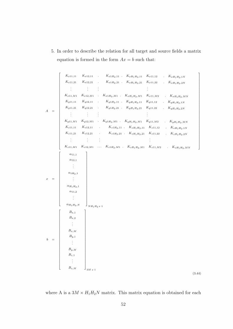
5. In order to describe the relation for all target and source fields a matrix

equation is formed in the form Ax = b such that:

A =

Kx11,11 Kx12,11 . Kx1H2,11 . KxH1H2,11 Kx11,12 . KxH1H2,1N

Kx11,21 Kx12,21 . Kx1H2,21 . KxH1H2,21 Kx11,22 . KxH1H2,2N

.

.....

.

.....

Kx11,M1 Kx12,M1 . Kx1H2,M1 . KxH1H2,M1 Kx11,M2 . KxH1H2,MN

Ky11,11 Ky12,11 . Ky1H2,11 . KyH1H2,11 Ky11,12 . KyH1H2,1N

Ky11,21 Ky12,21 . Ky1H2,21 . KyH1H2,21 Ky11,22 . KyH1H2,2N

..

....

..

....

Ky11,M1 Ky12,M1 . Ky1H2,M1 . KyH1H2,M1 Ky11,M2 . KyH1H2,MN

Kz11,11 Kz12,11 . Kz1H2,11 . KzH1H2,11 Kz11,12 . KzH1H2,1N

Kz11,21 Kz12,21 . Kz1H2,21 . KzH1H2,21 Kz11,22 . KzH1H2,2N

.

.....

.

.....

Kz11,M1 Kz12,M1 . . . Kz1H2,M1 . KzH1H2,M1 Kz11,M2 . KzH1H2,MN

x =

α11,1

α12,1

.

..

α1H2,1

.

..

αH1H2,1

α11,2

.

..

αH1H2,N

NH1H2 x 1

b =

Bx,1

Bx,2

.

..

Bx,M

By,1

...

By,M

Bz,1

..

.

Bz,M

3M x 1

(3.44)

where A is a 3M ×H1H2N matrix. This matrix equation is obtained for each

52

required RF Field definition and for each source geometry using MATLAB.

Implementations for the remaining three geometries are carried out in a sim-

ilar manner to planar surface modifying the target and source coordinates

and assigning the basis function parameters taking the boundary conditions

into consideration. However, matrix A is usually an ill-condition matrix and

therefore, the matrix solution has to be obtained using regularization methods.

3.5 Obtaining the Solution by Regularization

In order to obtain the solution matrix x, TSVD, Tikhonov, CGLS, TTLS,

Rutisbauer methods are implemented, the details of which are explained in

Appendix A.

In order to obtain minimum error and optimum solutions for each regular-

ization, the regularization parameters are swept,

1. For CGLS method, iteration number k is incremented from 1 to 3000 in

steps of one.

2. For Tikhonov Method, three different L matrices are evaluated (identity,

first derivative and second derivative) and regularization parameter λ is

evaluated as 10i and i is swept from 2 to -8 in decremented steps of 0,5.

3. For Rutisbauer Method, regularization parameter λ is evaluated as 10i

and i is swept from 2 to -8 in decremented steps of 0,5.

4. For TSVD Method, regularization parameter k is swept from 1 to 1800

in incremented steps of 30.

‖Ax‖ and ‖x‖ norms are evaluated for each value of the swept regularization

parameter for each

1. matrix A obtained for the geometry selection,

2. matrix b required field selection,

53

3. regularization method.

Using the L-Curve Method [46], optimum solution for the current density and

stream function coefficients are recorded and the average error percentages

between the required and generated magnetic field are calculated for each reg-

ularization method, source geometry and RF field case.

In order to decrease the complexity of the comparison process, the RF field

options, which turned out to yield high error percentages are eliminated and

the comparison process is carried out with RF field case 4.

Each solution is evaluated taking the error percentage and the realizability

of the coil into consideration. The stream function contours form the patterns

for the coil conductor, so it is the major measure of how realizable the coil is.

3.6 Approximating the Stream Function by a

Conductor

After the solution is obtained using one of the regularization parameters, the

coefficients can be substituted back into the basis functions in order to obtain

the current density distribution and stream functions for every subdomain.

The contours of the stream functions are used to determine the conductor

shape for the RF coil.

3.6.1 A simple Procedure

1. Choose the number of contour lines, Ns ∈ ℵ to describe the two dimen-

sional stream function on a surface S on xz plane.

2. Define the difference of current between two adjacent streamlines as:

∆I =maxx∈Sψ(x)−minx∈Sψ(x)

Ns

(3.45)

54

3. The centerlines of the unconnected conductors are the isolines of ψ(x)

with step ∆I,

x ∈ S | ψ(x) = minx∈Sψ(x) + (n− 1

2)∆I, n = 1, ..., Ns (3.46)

4. Form unconnected conductors from the centerlines by applying a width.

The width can be constrained by physical considerations or optimization

parameters.

5. Convert the unconnected conductors into one conductor by opening ends

of close loops and adding one end to another changing the streamline

shape as slightly as possible.

55

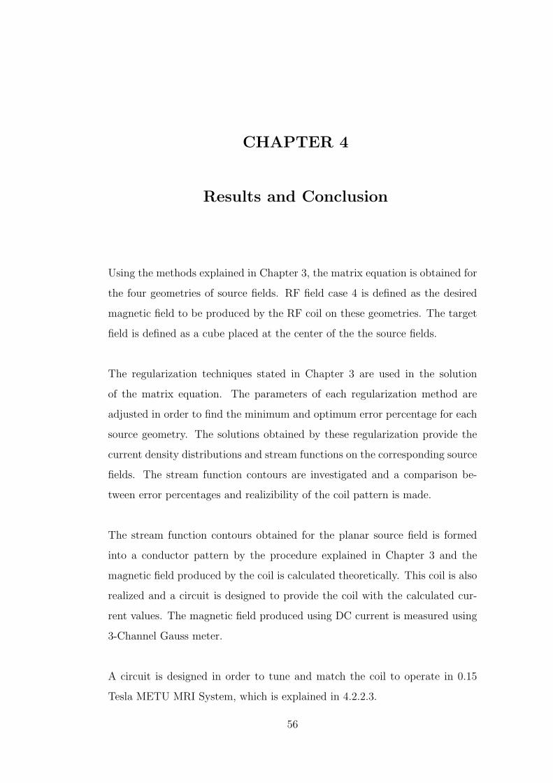
CHAPTER 4

Results and Conclusion

Using the methods explained in Chapter 3, the matrix equation is obtained for

the four geometries of source fields. RF field case 4 is defined as the desired

magnetic field to be produced by the RF coil on these geometries. The target

field is defined as a cube placed at the center of the the source fields.

The regularization techniques stated in Chapter 3 are used in the solution

of the matrix equation. The parameters of each regularization method are

adjusted in order to find the minimum and optimum error percentage for each

source geometry. The solutions obtained by these regularization provide the

current density distributions and stream functions on the corresponding source

fields. The stream function contours are investigated and a comparison be-

tween error percentages and realizibility of the coil pattern is made.

The stream function contours obtained for the planar source field is formed

into a conductor pattern by the procedure explained in Chapter 3 and the

magnetic field produced by the coil is calculated theoretically. This coil is also

realized and a circuit is designed to provide the coil with the calculated cur-

rent values. The magnetic field produced using DC current is measured using

3-Channel Gauss meter.

A circuit is designed in order to tune and match the coil to operate in 0.15

Tesla METU MRI System, which is explained in 4.2.2.3.

56

4.1 Theoretical Results

4.1.1 Desired and Generated Magnetic Fields

The minimum and optimum error percentages are calculated for each solution

obtained by the corresponding regularization method using the formula:

error % =

[∑Mi=1

(Bdesired,i−Bcalculated,i)2

B2desired,i

]

3M× 100 (4.1)

where M is the number of field points.

The error percentages for minimum error solution are illustrated in Table 4.1

while error percentages for optimum error solution are illustrated in Table 4.2.

Table 4.1: Error percentages for solutions with minimum error. Minimum errorpercentages between the desired and generated magnetic field are illustrated forthe current density solutions obtained by applying the regularization methodslisted as columns to source surfaces listed as rows for the corresponding targetfields.

CGLS Rutisbauer TSVD TikhonovL= Identity L=1stder. L=2ndder.

Planar 25,7 26,0 25,2 25,1 25,2 24,8Tri-Planar 3,8 4,1 3,8 3,8 3,7 3,83 Orth.Planes

11,2 12,0 2,5 2,5 2,4 2,2

Cylindrical 3,8 3,9 3,9 3,9 3,9 3,8

Table 4.2: Error percentages for solutions with optimum error. Error per-centages between the desired and generated magnetic field are illustrated forthe optimum current density solutions obtained by applying the regularizationmethods listed as columns to source surfaces listed as rows for the correspond-ing target fields.

CGLS Rutisbauer TSVD TikhonovL= Identity L=1stder. L=2ndder.

Planar 26,0 35,0 29,0 30,6 30,7 26,6Tri-Planar 4,3 9,5 5,0 6,6 8,4 4,23 Orth.Planes

12,1 29,9 3,2 3,7 4,6 6,1

Cylindrical 4,7 7,5 5,3 4,6 9,2 9,3

57

The regularization parameter values used in order to obtain the minimum and

optimum error solutions are stated in Table 4.3, Table 4.4, Table 4.5 and Table

4.6.

Table 4.3: Regularization parameter values for planar surface

PLANARMinimum Error Solution Optimum Error Solution

CGLS iteration number = 2305 iteration number = 273Rutisbauer λ = 3.162× 10−7 λ = 3.162× 10−3

TSVD truncation level = 691 truncation level = 181Tikhonov L= identity λ = 10−6 λ = 3.162× 10−2

L= 1st der. λ = 10−6 λ = 0.1L= 2nd der. λ = 10−3 λ = 0.01

Table 4.4: Regularization parameter values for tri-planar surface

TRI-PLANARMinimum Error Solution Optimum Error Solution

CGLS iteration number = 1294 iteration number = 165Rutisbauer λ = 10−8 λ = 3.162x10−4

TSVD truncation level = 661 truncation level = 61Tikhonov L= identity λ = 3.162× 10−7 λ = 0.01

L= 1st der. λ = 3.162× 10−7 λ = 0.1L= 2nd der. λ = 10−7 λ = 10−4

58

Table 4.5: Regularization parameter values for three orthogonal planes

THREE ORTHOGONAL PLANESMinimum Error Solution Optimum Error Solution

CGLS iteration number = 198;2789; 3000

iteration number = 162;331; 395

Rutisbauer λ = 10−8; 10−8; 10−8 λ = 10−4; 3.162 × 10−4;3.162× 10−4

TSVD truncation level = 301;451; 541

truncation level = 61; 61;91

Tikhonov L= identity λ = 10−7; 10−7; 10−7 λ = 10−4; 3.162 ×10−7; 10−3

L= 1st der. λ = 3.162 ×10−7; 10−7; 3.162× 10−7

λ = 10−3; 3.162 ×10−6; 0.01

L= 2nd der. λ = 3.162× 10−8; 3.162×10−8; 3.162× 10−8

λ = 3.162 ×10−4; 10−4; 10−4

Table 4.6: Regularization parameter values for cylindrical surface

CYLINDRICALMinimum Error Solution Optimum Error Solution

CGLS iteration number = 2984 iteration number = 52Rutisbauer λ = 10−8 λ = 0.3162TSVD truncation level = 661 truncation level = 61Tikhonov L= identity λ = 3.162× 10−6 λ = 3.162× 10−3

L= 1st der. λ = 10−5 λ = 10−2

L= 2nd der. λ = 3.162× 10−7 λ = 10−4

4.1.2 Stream Function Contours

The stream function contours resulting from the minimum and optimum error

solutions for each regularization method are illustrated in tables from Table

4.7 to Table 4.14.

59

Table 4.7: Stream function contours for planar surface - 1

PLANARMinimum Error Solution Optimum Error Solution

CGLS

Rutis.

TSVD

60

Table 4.8: Stream function contours for planar surface - 2

PLANARTikh. Minimum Error Solution Optimum Error Solution

L = I

L =1stder.

L =2ndder.

61

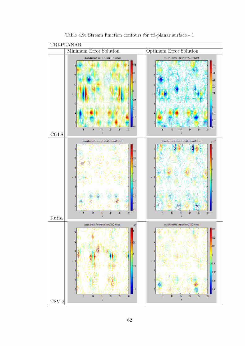
Table 4.9: Stream function contours for tri-planar surface - 1

TRI-PLANARMinimum Error Solution Optimum Error Solution

CGLS

Rutis.

TSVD

62

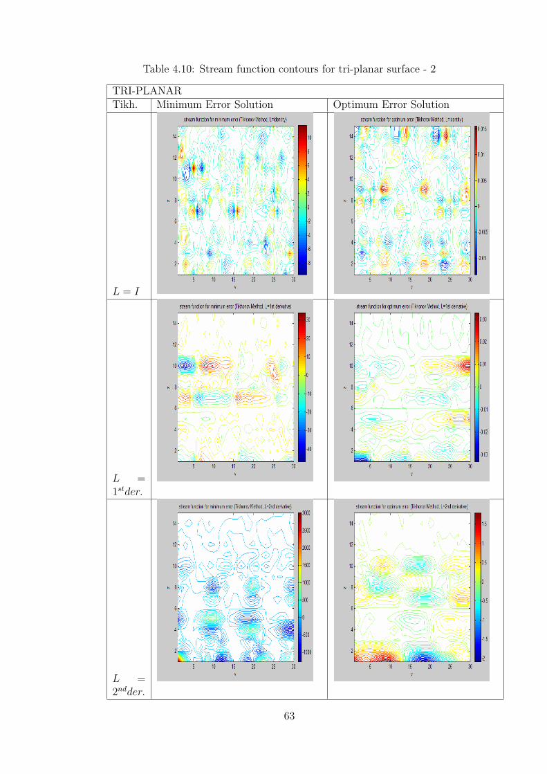
Table 4.10: Stream function contours for tri-planar surface - 2

TRI-PLANARTikh. Minimum Error Solution Optimum Error Solution

L = I

L =1stder.

L =2ndder.

63

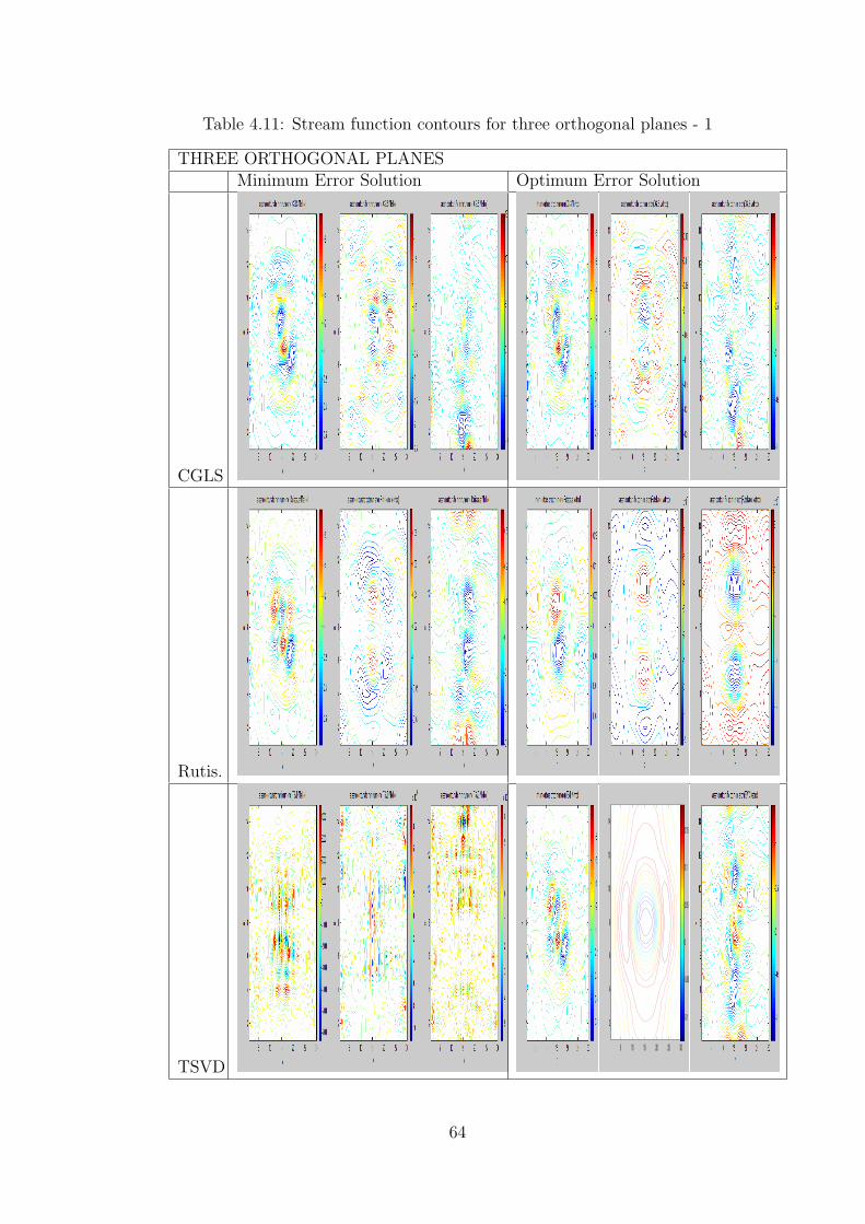
Table 4.11: Stream function contours for three orthogonal planes - 1

THREE ORTHOGONAL PLANESMinimum Error Solution Optimum Error Solution

CGLS

Rutis.

TSVD

5 10 15 20 25 30

2

4

6

8

10

12

14

-0.1

-0.05

0

0.05

0.1

0.15

64

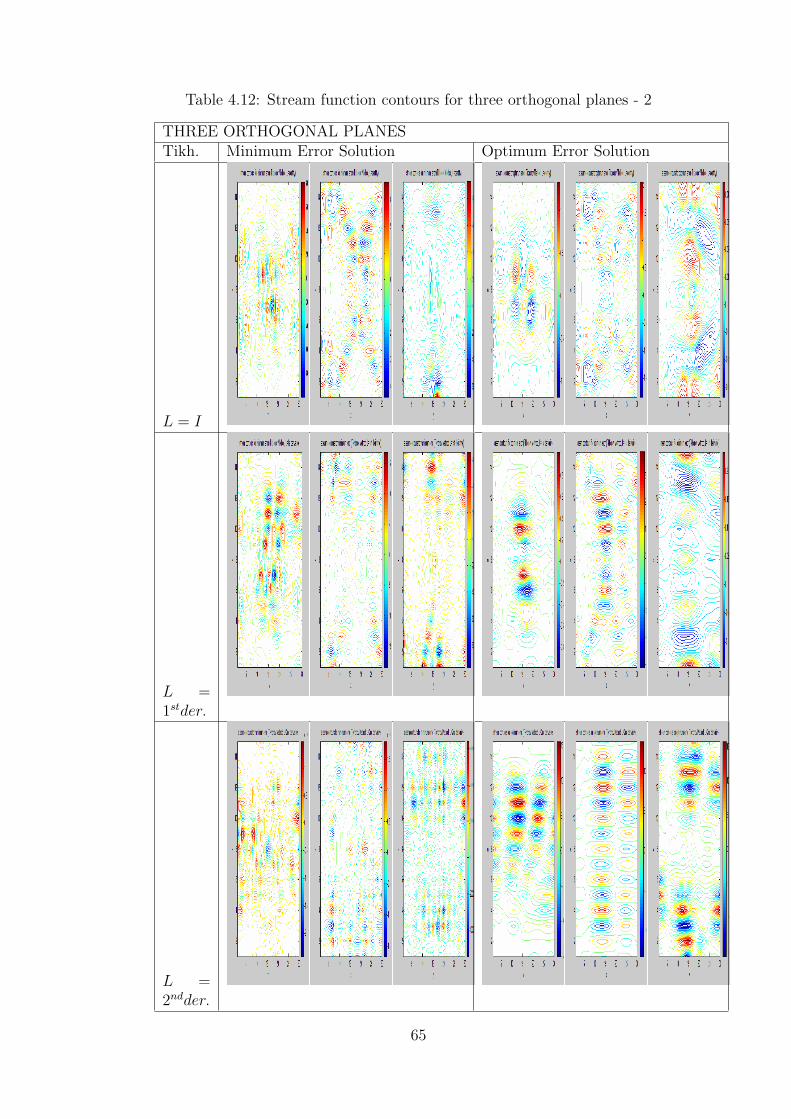
Table 4.12: Stream function contours for three orthogonal planes - 2

THREE ORTHOGONAL PLANESTikh. Minimum Error Solution Optimum Error Solution

L = I

L =1stder.

L =2ndder.

65

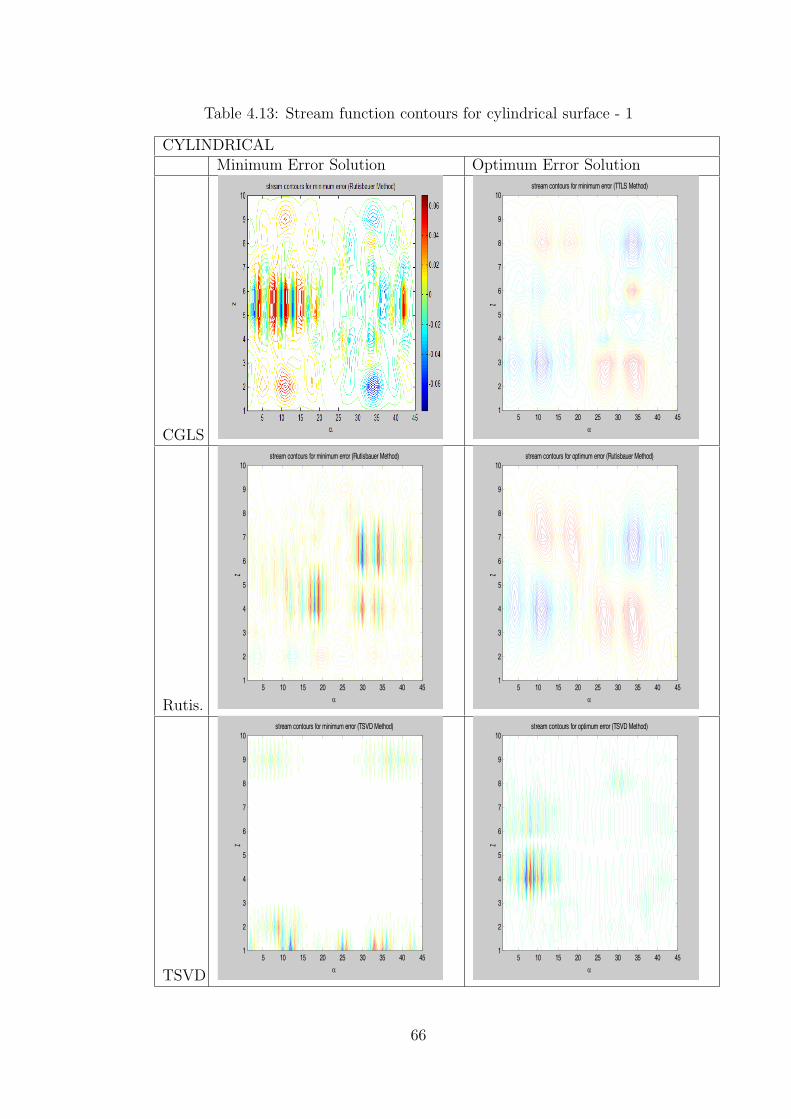
Table 4.13: Stream function contours for cylindrical surface - 1

CYLINDRICALMinimum Error Solution Optimum Error Solution

CGLS

stream contours for minimum error (TTLS Method)

α

z

5 10 15 20 25 30 35 40 451

2

3

4

5

6

7

8

9

10

Rutis.

stream contours for minimum error (Rutisbauer Method)

α

z

5 10 15 20 25 30 35 40 451

2

3

4

5

6

7

8

9

10stream contours for optimum error (Rutisbauer Method)

α

z

5 10 15 20 25 30 35 40 451

2

3

4

5

6

7

8

9

10

TSVD

stream contours for minimum error (TSVD Method)

α

z

5 10 15 20 25 30 35 40 451

2

3

4

5

6

7

8

9

10stream contours for optimum error (TSVD Method)

α

z

5 10 15 20 25 30 35 40 451

2

3

4

5

6

7

8

9

10

66

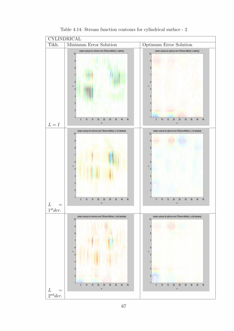
Table 4.14: Stream function contours for cylindrical surface - 2

CYLINDRICALTikh. Minimum Error Solution Optimum Error Solution

L = I

stream contours for minimum error (Tikhonov Method, L=identity)

α

z

5 10 15 20 25 30 35 40 451

2

3

4

5

6

7

8

9

10stream contours for optimum error (Tikhonov Method, L=identity)

α

z

5 10 15 20 25 30 35 40 451

2

3

4

5

6

7

8

9

10

L =1stder.

stream contours for minimum error (Tikhonov Method, L=1st derivative)

α

z

5 10 15 20 25 30 35 40 451

2

3

4

5

6

7

8

9

10stream contours for optimum error (Tikhonov Method, L=1st derivative)

α

z

5 10 15 20 25 30 35 40 451

2

3

4

5

6

7

8

9

10

L =2ndder.

stream contours for minimum error (Tikhonov Method, L=2nd derivative)

α

z

5 10 15 20 25 30 35 40 451

2

3

4

5

6

7

8

9

10stream contours for optimum error (Tikhonov Method, L=2nd derivative)

α

z

5 10 15 20 25 30 35 40 451

2

3

4

5

6

7

8

9

10

67

When the conductor patterns obtained using each regularization method for

each geometry are compared with reference to the complexity of patterns, the

optimum surface geometry is determined to be the cylindrical coil and the

optimum regularization method is chosen to be Rutisbauer, which produces

the conductor pattern illustrated in Figure 4.1.

stream contours for optimum error (Rutisbauer Method)

α

z

5 10 15 20 25 30 35 40 451

2

3

4

5

6

7

8

9

10

Figure 4.1: Stream function contours on the cylindrical surface for the solutionwith optimum error

4.2 Realizing the Coil

4.2.1 Orientation of Field Points

In order to illustrate the desired and created magnetic field values, 2-D plots

are used, which illustrate the magnetic field magnitudes at corresponding field

points. Figure 4.2 illustrates the orientation of the field points and which

number they symbolize on the magnetic field plot.

68

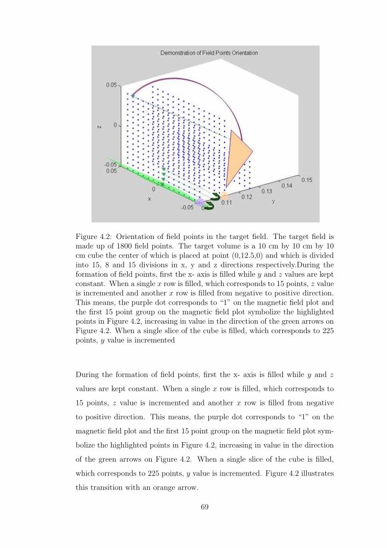
Figure 4.2: Orientation of field points in the target field. The target field ismade up of 1800 field points. The target volume is a 10 cm by 10 cm by 10cm cube the center of which is placed at point (0,12.5,0) and which is dividedinto 15, 8 and 15 divisions in x, y and z directions respectively.During theformation of field points, first the x- axis is filled while y and z values are keptconstant. When a single x row is filled, which corresponds to 15 points, z valueis incremented and another x row is filled from negative to positive direction.This means, the purple dot corresponds to “1” on the magnetic field plot andthe first 15 point group on the magnetic field plot symbolize the highlightedpoints in Figure 4.2, increasing in value in the direction of the green arrows onFigure 4.2. When a single slice of the cube is filled, which corresponds to 225points, y value is incremented

During the formation of field points, first the x- axis is filled while y and z

values are kept constant. When a single x row is filled, which corresponds to

15 points, z value is incremented and another x row is filled from negative

to positive direction. This means, the purple dot corresponds to “1” on the

magnetic field plot and the first 15 point group on the magnetic field plot sym-

bolize the highlighted points in Figure 4.2, increasing in value in the direction

of the green arrows on Figure 4.2. When a single slice of the cube is filled,

which corresponds to 225 points, y value is incremented. Figure 4.2 illustrates

this transition with an orange arrow.

69

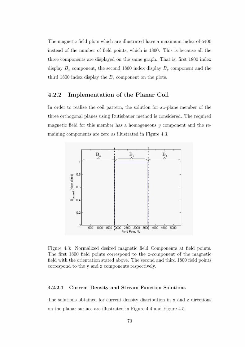
The magnetic field plots which are illustrated have a maximum index of 5400

instead of the number of field points, which is 1800. This is because all the

three components are displayed on the same graph. That is, first 1800 index

display Bx component, the second 1800 index display By component and the

third 1800 index display the Bz component on the plots.

4.2.2 Implementation of the Planar Coil

In order to realize the coil pattern, the solution for xz-plane member of the

three orthogonal planes using Rutisbauer method is considered. The required

magnetic field for this member has a homogeneous y component and the re-

maining components are zero as illustrated in Figure 4.3.

Figure 4.3: Normalized desired magnetic field Components at field points.The first 1800 field points correspond to the x-component of the magneticfield with the orientation stated above. The second and third 1800 field pointscorrespond to the y and z components respectively.

4.2.2.1 Current Density and Stream Function Solutions

The solutions obtained for current density distribution in x and z directions

on the planar surface are illustrated in Figure 4.4 and Figure 4.5.

70

Figure 4.4: Magnitude of Jx solution for the planar surface on xz-plane. Thecenter of the planar surface of dimensions 30 cm by 30 cm is placed at (x=0,z=0) on xz-plane. The magnitude of J is expressed in A/m.

Figure 4.5: Magnitude of Jz solution for the planar surface on xz-plane. Thecenter of the planar surface of dimensions 30 cm by 30 cm is placed at (x=0,z=0) on xz-plane. The magnitude of J is expressed in A/m.

71

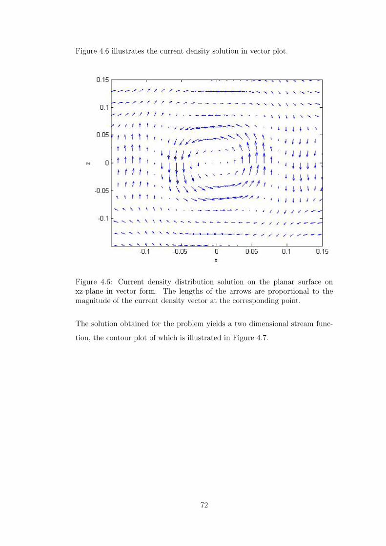
Figure 4.6 illustrates the current density solution in vector plot.

Figure 4.6: Current density distribution solution on the planar surface onxz-plane in vector form. The lengths of the arrows are proportional to themagnitude of the current density vector at the corresponding point.

The solution obtained for the problem yields a two dimensional stream func-

tion, the contour plot of which is illustrated in Figure 4.7.

72

Figure 4.7: Stream function solution for the current density distribution on thexz-plane. x and z axis represent the coordinates of the points on the planarsurface in meters. The stream function is represented with 25 streamlines.

The stream function solution is considered using 6 streamlines as illustrated

in Figure 4.8.

73

Figure 4.8: Streamlines for the stream function solution on the xz-Plane. xand z axis represent the coordinates of the points on the planar surface inmeters. The stream function is represented with 6 streamlines.

4.2.2.2 Comparing the Desired, Generated and Measured Fields

The magnetic field calculated using the current density distribution solution

is illustrated in Figure 4.9. The average error percentage between the y com-

ponent of the desired and the generated magnetic field using current density

distributions is calculated to be 4.38%.

74

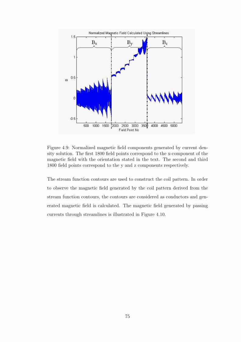
Figure 4.9: Normalized magnetic field components generated by current den-sity solution. The first 1800 field points correspond to the x-component of themagnetic field with the orientation stated in the text. The second and third1800 field points correspond to the y and z components respectively.

The stream function contours are used to construct the coil pattern. In order

to observe the magnetic field generated by the coil pattern derived from the

stream function contours, the contours are considered as conductors and gen-

erated magnetic field is calculated. The magnetic field generated by passing

currents through streamlines is illustrated in Figure 4.10.

75

Figure 4.10: Normalized magnetic field components generated using stream-lines. Streamlines are considered as conductor wires. The first 1800 fieldpoints correspond to the x-component of the magnetic field with the orienta-tion stated above. The second and third 1800 field points correspond to the yand z components respectively.

The average error percentage between the y component of the desired and the

generated magnetic field using stream lines is calculated to be 6.83%.

4.2.2.3 Constructing the Coil and the Circuitry

The streamlines illustrated in Figure 4.8 are utilized as explained in Chapter

3 to construct a conductor pattern for the RF coil. The conductor pattern is

produced using AutoCAD and the design illustrated in Figure 4.11 is realized

by etching of FR4 plates. The realized coil is illustrated in Figure 4.12

76

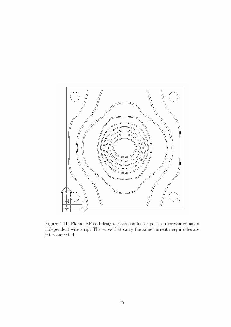
Figure 4.11: Planar RF coil design. Each conductor path is represented as anindependent wire strip. The wires that carry the same current magnitudes areinterconnected.

77

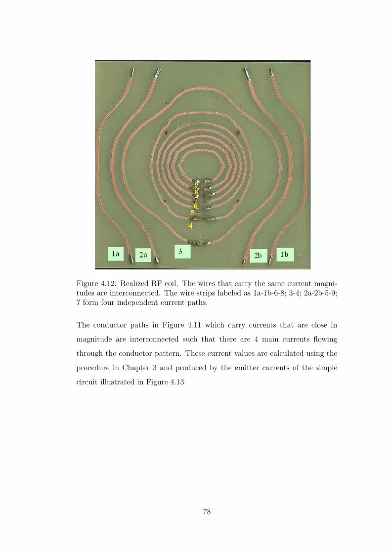
Figure 4.12: Realized RF coil. The wires that carry the same current magni-tudes are interconnected. The wire strips labeled as 1a-1b-6-8; 3-4; 2a-2b-5-9;7 form four independent current paths.

The conductor paths in Figure 4.11 which carry currents that are close in

magnitude are interconnected such that there are 4 main currents flowing

through the conductor pattern. These current values are calculated using the

procedure in Chapter 3 and produced by the emitter currents of the simple

circuit illustrated in Figure 4.13.

78

Figure 4.13: Circuit to provide DC currents. The currents to feed the RF coilwire are obtained by the emitter currents of each branch.

79

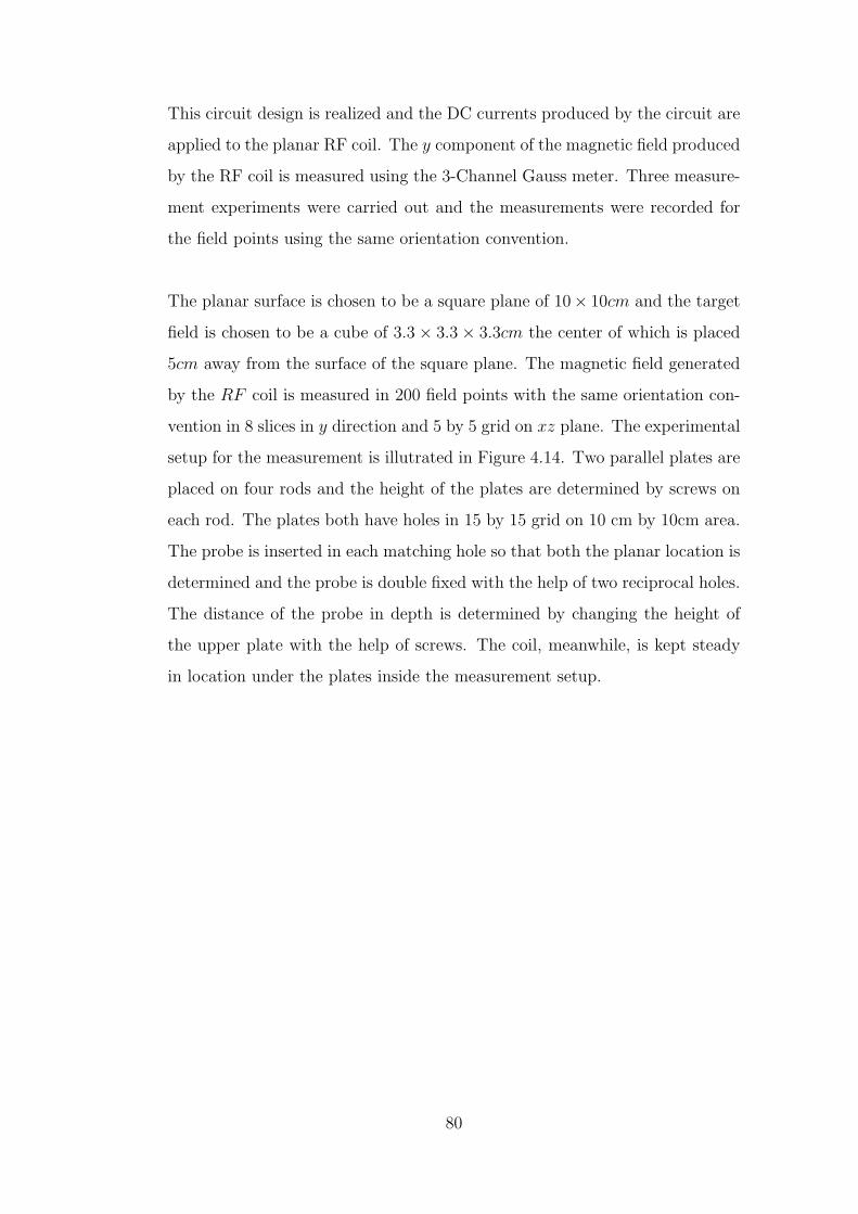
This circuit design is realized and the DC currents produced by the circuit are

applied to the planar RF coil. The y component of the magnetic field produced

by the RF coil is measured using the 3-Channel Gauss meter. Three measure-

ment experiments were carried out and the measurements were recorded for

the field points using the same orientation convention.

The planar surface is chosen to be a square plane of 10× 10cm and the target

field is chosen to be a cube of 3.3× 3.3× 3.3cm the center of which is placed

5cm away from the surface of the square plane. The magnetic field generated

by the RF coil is measured in 200 field points with the same orientation con-

vention in 8 slices in y direction and 5 by 5 grid on xz plane. The experimental

setup for the measurement is illutrated in Figure 4.14. Two parallel plates are

placed on four rods and the height of the plates are determined by screws on

each rod. The plates both have holes in 15 by 15 grid on 10 cm by 10cm area.

The probe is inserted in each matching hole so that both the planar location is

determined and the probe is double fixed with the help of two reciprocal holes.

The distance of the probe in depth is determined by changing the height of

the upper plate with the help of screws. The coil, meanwhile, is kept steady

in location under the plates inside the measurement setup.

80

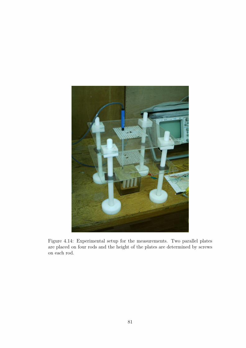
Figure 4.14: Experimental setup for the measurements. Two parallel platesare placed on four rods and the height of the plates are determined by screwson each rod.

81

The normalized magnetic field results for each measurement are illustrated in

Figure 4.15, 4.16 and 4.17. The magnetic field values measured for the RF

coil are compared to the theoretical values at the corresponding field points

which is illustrated in Figure 4.18.

Figure 4.15: Normalized measured magnetic field - Measurement 1. y-component of the magnetic field is measured using the LakeShore 3-ChannelGaussmeter. The target volume is a cube of dimensions 3.3cm by 3.3cm by3.3cm. The target volume is divided into 5, 8 and 5 divisions in x, y and zdirections respectively yielding 200 field points

82

Figure 4.16: Normalized measured magnetic field - Measurement 2. Secondmeasurement is done on the y-component of the magnetic field using theLakeShore 3-Channel Gaussmeter under similar conditions.

Figure 4.17: Normalized measured magnetic field - Measurement 3. Third mea-surement is done on the y-component of the magnetic field using the LakeShore3-Channel Gaussmeter under similar conditions.

83

Figure 4.18: Calculated magnetic field. y-component of the magnetic field iscalculated considering the streamlines as conductor paths. The target volumeis a cube of dimensions 3.3cm by 3.3cm by 3.3cm. The target volume is dividedinto 5, 8 and 5 divisions in x, y and z directions respectively yielding 200 fieldpoints

84

The error percentages between the measured and calculated magnetic field

values are calculated using Equation 4.1, which are stated in Table 4.15.

Table 4.15: Error percentages between desired, calculated and measured Fields

Measurement 1 Measurement 2 Measurement 3Error % between thecalculated and measuredfields

2.13 % 1.98 % 1.92 %

Error % between the de-sired and measured fields

9.78 % 7.26 % 5.21 %

4.2.3 Tuning and Matching the RF Coil

As the RF Coil is designed to operate in 0.15 Tesla MRI system, it should be

tuned to 6.387 MHz and matched to 50 Ohms. Another requirement on the

RF coil is that four conductor paths should carry different currents. Therefore,

each branch is matched to a real impedance such that it passes the required

current and the resultant impedance matches 50 Ohms.

1. In order to measure the inductance of each conductor path, an RLC

circuit is set up where each conductor path is connected in series with a

resistor of 1Ω and a variable capacitance of 1pF sensitivity.

2. The voltage on the resistance is measured by the 54622D Mixed Signal

Oscilloscope increasing the capacitance value at a constant frequency.

3. Maximum voltage amplitude on the resistor is determined where capac-

itance totally cancels inductance.

4. Fine tuning is accomplished by the varying the frequency value.

5. The capacitance value at the maximum voltage is recorded and used to

calculate the inductance value according to the formula:

L =1

w2C(4.2)

6. Inductance of each conductor path is calculated as stated in Table 4.16.

85

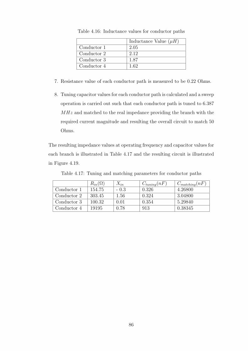
Table 4.16: Inductance values for conductor paths

Inductance Value (µH)Conductor 1 2.05Conductor 2 2.12Conductor 3 1.87Conductor 4 1.62

7. Resistance value of each conductor path is measured to be 0.22 Ohms.

8. Tuning capacitor values for each conductor path is calculated and a sweep

operation is carried out such that each conductor path is tuned to 6.387

MHz and matched to the real impedance providing the branch with the

required current magnitude and resulting the overall circuit to match 50

Ohms.

The resulting impedance values at operating frequency and capacitor values for

each branch is illustrated in Table 4.17 and the resulting circuit is illustrated

in Figure 4.19.

Table 4.17: Tuning and matching parameters for conductor paths

Rin(Ω) Xin Ctuning(nF ) Cmatching(nF )Conductor 1 154.75 - 0.3 0.326 4.26800Conductor 2 303.45 1.56 0.324 3.04800Conductor 3 100.32 0.01 0.354 5.29840Conductor 4 19195 0.78 913 0.38345

86

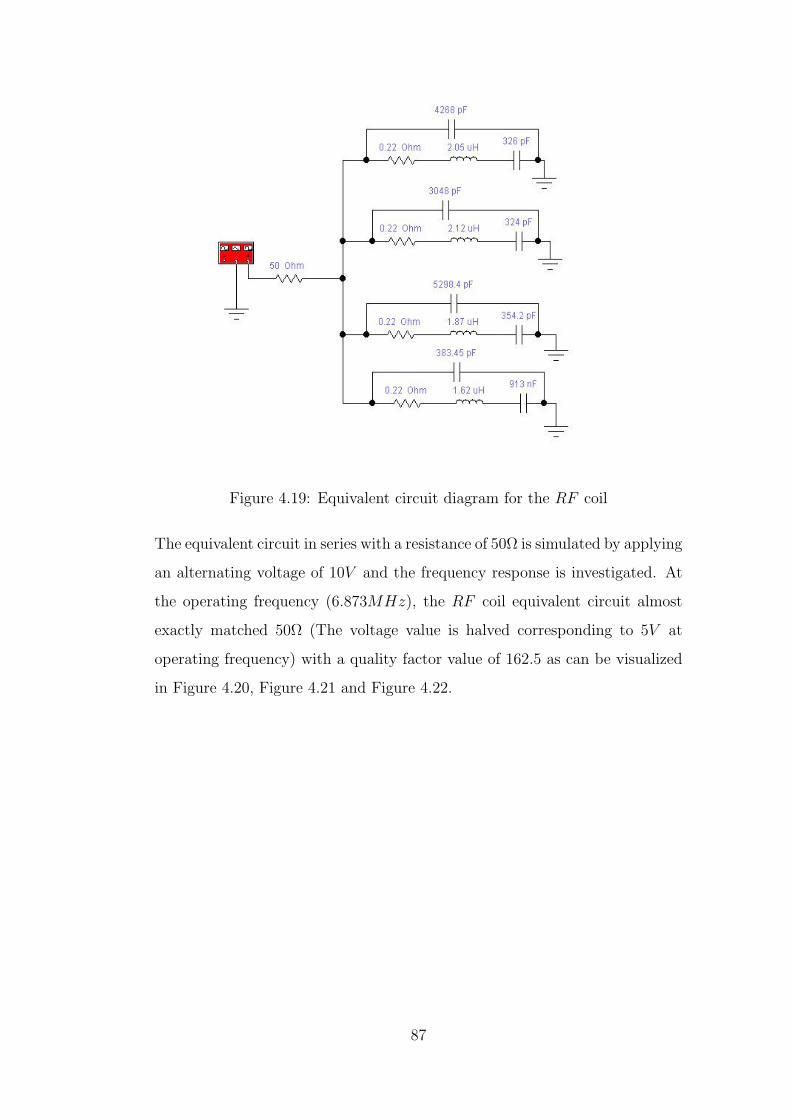
Figure 4.19: Equivalent circuit diagram for the RF coil

The equivalent circuit in series with a resistance of 50Ω is simulated by applying

an alternating voltage of 10V and the frequency response is investigated. At

the operating frequency (6.873MHz), the RF coil equivalent circuit almost

exactly matched 50Ω (The voltage value is halved corresponding to 5V at

operating frequency) with a quality factor value of 162.5 as can be visualized

in Figure 4.20, Figure 4.21 and Figure 4.22.

87

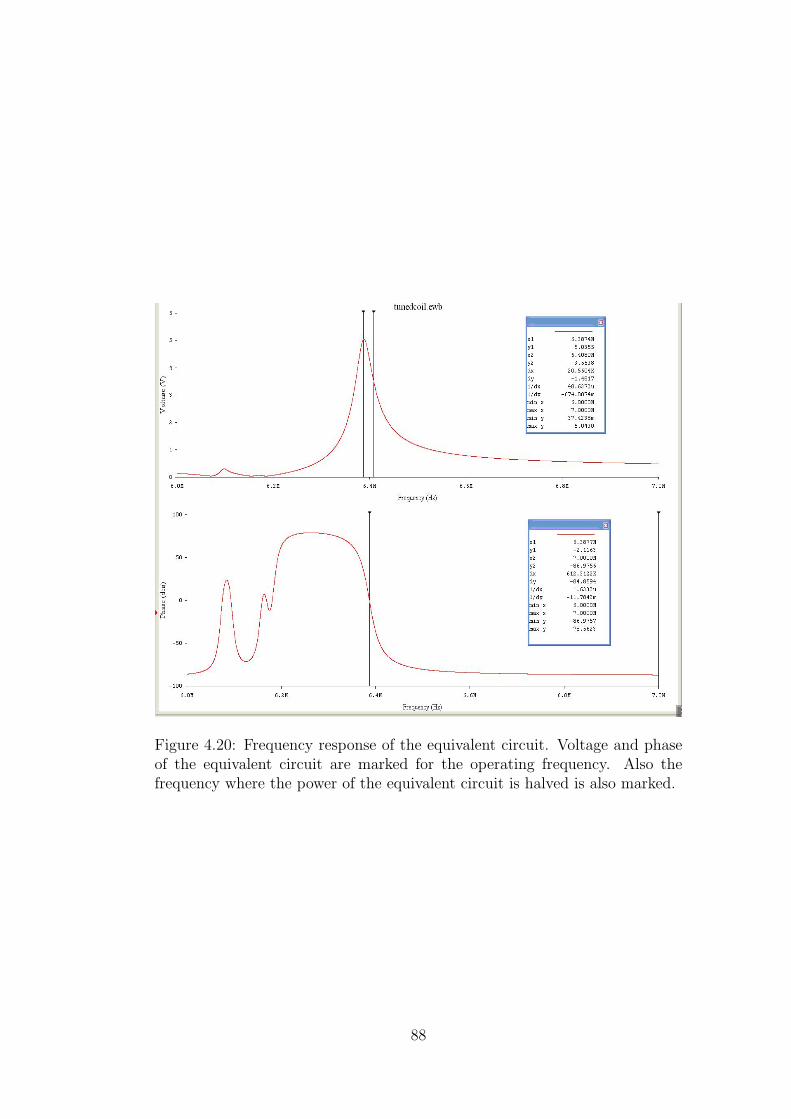
Figure 4.20: Frequency response of the equivalent circuit. Voltage and phaseof the equivalent circuit are marked for the operating frequency. Also thefrequency where the power of the equivalent circuit is halved is also marked.

88

Figure 4.21: Voltage magnitude on the equivalent circuit at the operatingfrequency when the coil is considered to be connected in series with a resistanceof 50 Ω. At 6.387MHz, the applied voltage of 10V is divided into two; in otherwords, the coil is matched to 50 Ω.

Figure 4.22: The phase of the equivalent circuit at the operating frequencywhen the coil is considered to be connected in series with a resistance of 50Ω. At 6.387MHz, the phase of the equivalent circuit is nearly zero; in otherwords, the coil is tuned to 50 Ω.

89

4.3 Conclusion

Using the algorithm provided in this study, the source and field geometries can

be defined as any geometry providing a source field that surrounds or fits a

particular part of the patient and a target field that constitutes the volume of

an inner part of the body like an organ, vessel... etc.

When the error between the desired and generated magnetic fields is con-

sidered, the desired magnetic field is theoretically obtained within acceptable

error ranges for several source geometries using regularization methods of dif-

ferent characteristics. However, the characteristics of the required magnetic

field affect the success of the algorithm. In other words, any kind of magnetic

field can not be created with an error within acceptable limits. Magnetic fields

that are more likely to be produced by a surface current density, based on the

current density and magnetic field mathematical relations, are created with

smaller errors. Magnetic fields that have more homogenous characteristics

are created with much less errors than the ones with inhomogeneous charac-

teristics. This is attributed to the averaging effect of regularization algorithms.

Besides, three dimensional surface models give better results for the same

required magnetic fields. This is attributed to the compensation of additional

surfaces, which are located orthogonally to the single planar surface, to the

radically decreasing characteristics of the magnetic field. The tri-planar sur-

face model and orthogonally placed planar surfaces model give similar results

for the same magnetic field inputs. However, the problem is solved indepen-

dently for each coil for the orthogonally placed planar surfaces model. It is

speculated that the error between the desired magnetic field and the created

field can be diminished by solving the problem when the surfaces are specified

to be dependent on each other. The minimum and optimum average error

percentage values were smallest for cylindrical surface model for every regu-

larization method.

90

When current density solutions are considered, the current density distribu-

tions producing the minimum average error percentages are harder to imple-

ment due to the high magnitude values than the ones producing the optimum

average error percentages which have relatively smaller magnitudes.

Stream functions are proved to be reliable tools to provide the conductor pat-

tern to produce the calculated current distribution. The coil patterns corre-

sponding to the current density distributions producing the minimum average

error percentages are harder to implement than the ones corresponding to the

current density distributions producing the optimum average error percentages

for each regularization method.

When conductor pattern solutions with reference to the utilized regulariza-

tion method are compared, the conductor pattern solutions using Rutisbauer

Method are easier to implement. When conductor pattern solutions with ref-

erence to the utilized source field geometry are compared, the coil patterns

computed for the tri-planar surface by the regularization methods are hard to

implement even though the average error percentages are very small.

When the RF coil pattern is realized for the planar coil and the generated

magnetic field is both theoretically calculated and experimentally measured,

the conductor patterns obtained using stream functions proved both theoret-

ically and experimentally to generate the calculated magnetic fields with a

small error.

During the simulation of the circuitry used to tune and match the coil, it

is seen that the capacitance values that yield the tuning and matching con-

ditions are very sensitive to small changes. When compared to tuning and

matching a conventional RF coil, tuning and matching process is harder to

implement as different current magnitudes on conductor branches with differ-

ent matching requirements should be accomplished at the same time. This

91

requires accurate measurement of the inductance values and capacitances the

magnitudes of which can be changed in very small steps.

4.4 Future Work

• The errors on the solenoidal characteristics of the current density due to

discritization of the fields on source geometries are aimed to be dimin-

ished by increasing the source points which will require parallel process-

ing and iterative algorithms.

• Genetic algorithm is aimed to be adapted to the problem in order to

obtain smaller errors with more realizable patterns.

• The signal obtained using the theoretical and experimental magnetic field

outcome is aimed to be simulated in an MRI simulator.

• The coil which is realized is aimed to be tuned to multiple frequencies.

• The coil is aimed to be experimented in METU MRI system.

• The coil is aimed to be experimented in inhomogeneous magnetic fields.

• A hand-held MRI scanner is aimed to be implemented and manufactured.

92

CHAPTER 5

Publications

5.1 Publications Prior to M. Sc. Study

H. Yigitler, A. Ozan Yılmaz, B. Murat Eyuboglu, ”An approach to geometrical

design of permanent magnets for biomedical applications”, 11th. International

Biomedical Science and Technology Days, Ankara - Turkey, p.24, 2004.

5.2 Publications during M. Sc. Study

A. Ozan Yılmaz, B. Murat Eyuboglu,”Homojen Olmayan Ana Manyetik Alanda

Manyetik Rezonans Goruntuleme icin RF sargısı Tasarımı” Proc. of URSI-

Turkiye 2006 3rd National Congress, Ankara - TR, pp.207-9, 2006

A. Ozan Yılmaz, B. Murat Eyuboglu, ”RF Coil Design for MRI Applications

in Inhomogeneous Main Magnetic Fields”, World Congress 2006, Seoul-Korea,

p.3084, August 2006.

93

REFERENCES

[1] F. Bloch, “Nuclear induction,” Physical Review, vol. 70, pp. 460–474,1946.

[2] F. Bloch, W. W. Hansen, and M. Packard, “The nuclear induction exper-iment,” Physical Review, vol. 70, pp. 474–485, 1946.

[3] E. M. Purcell, H. C. Torrey, and R. V. Pound, “Resonance absorption bynuclear magnetic moments in a solid,” Physical Review, vol. 69, pp. 37–38,1946.

[4] P. C. Lauterbur, “Image formation by induced local interactions - exam-ples employing nuclear magnetic-resonance,” Nature, vol. 242, pp. 190–191, 1973.

[5] R. Damadian, M. Goldsmith, and L. Minkoff, “Nmr in cancer: Xvi. fonarimage of the live human body,” Physiological Chemistry and Physics,vol. 9, pp. 97–100, 1977.

[6] F. Balibanu, K. Hailu, R. Eymael, D. E. Demco, and B. Blumich, “Nu-clear magnetic resonance in inhomogeneous magnetic fields,” Journal ofMagnetic Resonance, vol. 145, pp. 246–258, 2000.

[7] S. Anferova, V. Anferov, M. Adams, P. Blumler, N. Routley, K. Hailu,K. Kupferschlager, M. Malett, G. Schroeder, S. Sharma, and B. Blumich,“Nuclear magnetic resonance in inhomogeneous magnetic fields,” Con-cepts in Magnetic Resonance, vol. 15, pp. 15–25, 2002.

[8] F. Casanova and B. Blumich, “Two dimensional imaging with single-sidednmr probe,” Journal of Magnetic Resonance, vol. 163, pp. 38–45, 2003.

[9] J. Perlo, F. Casanova, and B. Blumich, “3d imaging with a single-sidedsensor: an open tomograph,” Journal of Magnetic Resonance, vol. 166,pp. 228–235, 2004.

[10] M. Brown, D. Verganelakis, M. Mallett, J. Mitchell, and P. Blumler, “Sur-face normal imaging with a hand-held nmr device,” Journal of MagneticResonance, vol. 169, pp. 308–312, 2004.

[11] P. J. Prado, “Single sided imaging sensor,” Magnetic Resonance Imaging,vol. 21, pp. 397–400, 2003.

94

[12] D. A. Thayer, “Imaging techniques and hardware for inhomogeneous mri,”Master’s thesis, Brigham Young University, December 2004.

[13] H. Yigitler, “Permanent magnet design and image reconstruction tech-nique for magnetic resonance imaging in inhomogeneous magnetic fields,”Master’s thesis, Middle East Technical University, September 2006.

[14] C. E. Hayes, W. A. Edelstein, J. F. Schenck, O. M. Mueller, and M. Eash,“An efficient, highly homogeneous radiofrequency coil for whole-body nmrimaging at 1.5t,” Journal of Magnetic Resonance, vol. 63, pp. 622–628,1985.

[15] J. Tropp, “The theory of the bird-cage resonator,” Journal of MagneticResonance, vol. 82, pp. 51–62, 1989.

[16] J. Tropp, “The theory of an arbitrary perturbed bird-cage resonator, anda simple method for restoring it to full symmetry,” Journal of MagneticResonance, vol. 95, pp. 235–243, 1991.

[17] F. D. Doty, G. Entzminger, and C. D. Hauch, “Error-tolerant rf litz coilsfor nmr/mri,” Journal of Magnetic Resonance, vol. 140, pp. 17–31, 1999.

[18] D. A. Roberts, E. K. Insko, L. Bolinger, and J. S. Leigh, “The theoryof an arbitrary perturbed bird-cage resonator, and a simple method forrestoring it to full symmetry,” Journal of Magnetic Resonance, vol. A102,pp. 34–41, 1993.

[19] J. Jin, Electromagnetic Analysis and Design in Magnetic Resonance Imag-ing. FL CRC, 1999.

[20] D. Ballon, S. M. M. C. Graham, and J. A.Koutcher, “A64 mhz half-birdcage resonator for clinical imaging,” Journal of Magnetic Resonance,vol. 90, pp. 131–140, 1990.

[21] J. Gasson, I. R. Summers, M. E. Fry, and W.Vennart, “Modified birdcagecoils for target imaging,” Mag. Reson. Imag., vol. 13, pp. 1003–1012, 1995.

[22] K. L. Zakian, J. A. Koutcher, and D. Ballon, “A dual-tuned resonatorfor proton-decoupled phosphorus-31 chemical shift imaging of the brain,”Magn. Reson. Med., vol. 41, no. 4, pp. 809–815, 1999.

[23] K. L. Meyer, K. Kim, T. Li, P. K. Tulipano, K. M. Lee, R. DeLaPaz,J. Hirsch, and D. Ballon, “Sensitivity-enhanced echo-planar mri at 1.5 tusing a 5x5 mesh dome resonator,” Magn. Reson. Med., vol. 36, no. 4,pp. 606–612, 1996.

[24] D. A. Molyneux and A. H. Qureshi, “Quadrature coil system for simul-taneous reception,” IEEE Transactions on Magnetics, vol. 29, pp. 2470–2472, November 1993.

95

[25] D. A. Molyneux and A. H. Qureshi, “Quadrature coil system for simul-taneous reception,” IEEE Transactions on Magnetics, vol. 32, pp. 5124–5126, September 1996.

[26] R. F. Lee, C. R. Westgate, R. G. Weiss, D. C. Newman, and P. A. Bot-tomley, “Planar strip array for mri,” Magnetic Resonance in Medicine,vol. 45, pp. 673–683, 2001.

[27] Z. Zhang, K. Ugurbil, and W. Chen, “Microstrip rf surface coil designfor extremely high-field mri and spectroscopy,” Magnetic Resonance inMedicine, vol. 46, pp. 443–450, 2001.

[28] Q. Y. Ma, “Rf applications of high temperature superconductors in mhzrange,” IEEE Transactions on Applied Superconductivity, vol. 9, pp. 3565–3568, June 1999.

[29] Q. Y. Ma, K. C. Chan, D. F. Kacher, E. Gao, M. S. Chow, K. K. Wong,H. Xu, E. S. Yang, G. S. Young, J. R. Miller, and F. A. Jolesz, “Supercon-ducting rf coils for clinical mr imaging at low field,” Acad Radiol, vol. 10,pp. 978–987, 2003.

[30] J.-C. Ginefri, L. Darrasse, and P. Crozat, “High-temperature supercon-ducting surface coil for in vivo microimaging of the human skin,” MagneticResonance in Medicine, vol. 45, pp. 376–382, 2001.

[31] M. A. Martens, L. S. Petropoulos, R. Brown, and J. H. Andrews, “In-sertable biplanar gradient coils for magnetic resonance imaging,” Rev.Sci. Instrum., vol. 62, pp. 2639–2645, Nov 1991.

[32] H. Fujita, L. S. Petropoulos, M. A. Morich, S. M. Shvartsman, and R. W.Brown, “A hybrid inverse approach applied to the design of lumpedele-ment rf coils,” IEEE Trans. Biomed. Eng., vol. 46, pp. 353–361, Mar1999.

[33] B. G. Lawrence, S. Crozier, D. Yau, and D. Doddrell, “A time-harmonicinverse methodology for the design of rf coils in mri,” IEEE Trans.Biomed. Eng., pp. 64–71, Jan 2002.

[34] B. G. Lawrence, S. Crozier, G. Cowin, and D. D. Yau, “An inverse designof an open, head/neck rf coil for mri,” IEEE Trans. Biomed. Eng., vol. 49,pp. 1024–1030, September 2002.

[35] P. T. While, L. K. Forbes, and S. Crozier, “A time-harmonic target-fieldmethod for designing unshielded rf coils in mri,” Measurement Scienceand Technology, vol. 16, pp. 997–1006, 2005.

[36] L. T. Muftuler, G. Chen, and O. Nalcıoglu, “An inverse method to de-sign rf coil arrays optimized for sense imaging,” Physics in Medicine andBiology, vol. 51, pp. 6457–6469, 2006.

96

[37] Z.-P. Liang and P. C. Lauterbur, Principles of Magnetic Resonance Imag-ing. IEEE.

[38] J. Pauly, D. Nishimura, and A. Macovski, “A k-space analysis of small-tip-angle excitation,” Journal of Magnetic Resonance, vol. 81, pp. 43–56,1989.

[39] R. F. Harrington, Field Computation by Moment Methods. The Machmil-lan Company, 1968.

[40] D. K. Cheng, Field and Wave Electromagnetics. Addison-Wesley Com-pany.

[41] M. A. Bridgeson, L. K. Forbes, and S. Crozier, “Determining complicatedwinding patterns for shim coils using stream functions and the target-fieldmethod,” Concepts Magn. Reson., vol. 14, pp. 9–18, 2002.

[42] O. C. Lingjearde and N. Christophersen, Regularization Principles SolvingIll-Posed Inverse Problems. September 1998.

[43] R. J. L. Montero, Pulse-Echo Image Formation using non-quadratic reg-ularization with speckle-based images. Pontificia Universidad Catolica delPeru, 2002.

[44] G. Mallinson, “The calculation of the lines of a three dimensional vectorfield,” Computation Fluid Mechanics, pp. 525–534, 1988.

[45] D. Knight and G. Mallinson, “Visualizing unstructured flow data usingdual stream functions,” IEEE Transactions on Visualization and Com-puter Graphics, vol. 2, pp. 355–363, December 1996.

[46] P. C. Hansen, Rank-Deficient and Discrete Ill-Posed Problems: NumericalAspects of Linear Inversion. SIAM.

[47] J. P. Reilly, “Matrix computations for signal processing.” Departmentof Electrical and Computer Engineering, McMaster University, February1998.

[48] G. H. Golub and C. F. V. Loan, Matrix Computations. the Johns HopkinsUniversity Press, 3 ed., 1996.

[49] A. J. Laub, Matrix Analysis for Scientists and Engineers. SIAM.

[50] H. Zha and P. C. Hansen, “Regularization and the general gauss-markovlinear model,” Physics in Medicine and Biology, vol. 55, pp. 613–624,October 1990.

[51] C. Paige, “Fast numerically stable computations for generalized linearleast squares problems,” SIAM Journal on Numerical Analysis, vol. 16,pp. 165–171, February 1979.

97

[52] G. H. Golub, P. C. Hansen, and D. P. O’Leary, “Tikhonov regularizationand total least squares,” SIAM Journal on Numerical Analysis, vol. 16,pp. 165–171, February 1979.

98

APPENDIX A

Regularization

A.1 Singular Value Decomposition

Every matrix A ∈ Rm,n has a SVD:

A = U0D0VT0 =

(UU

) D 0

0 0

V T

V T

= UDV T (A.1)

where U0 ∈ Rn,n and V0 ∈ Rm,m are orthogonal (i.e. UT0 U0 = I and V T

0 V0 = I)

and U ∈ Rm,r , D ∈ Rr,r and V ∈ Rm,r, where r ≤ min (n,m) is the rank of

A . The diagonal matrix D , has nonnegative diagonal elements appearing in

non increasing order such that

σ1 ≥ σ2 ≥ · · · ≥ σr > 0 (A.2)

Let u1, u2, . . . , un denote the column vectors of U0 and v1, v2, . . . , vm the col-

umn vectors of V0 . Then, u1, u2, . . . , ur span <(A) , ur+1, u2, . . . , un span

N(AT ) , v1, v2, . . . , vr span <(AT ) and vr+1, v2, . . . , vm span N(A) . It can be

observed that v1, v2, . . . , vm are the eigenvectors of AT A while u1, u2, . . . , un

are the eigenvectors of AAT . Furthermore, σ21, . . . , σ

2r are the non-zero eigen-

values of these matrices.

If the mapping Ax of an arbitrary vector x is considered, using the SVD

99

x =n∑

i=1

(vT

i x)

vi (A.3)

Ax =n∑

i=1

σi

(vT

i x)

ui (A.4)

these relations clearly show that due to multiplication with the σi , the high

frequency components of x are more damped in Ax than the low frequency

components. Moreover, the inverse problem, that computes x from Ax = b or

min ‖Ax− b‖2 , must have the opposite effect; it amplifies the high-frequency

oscillations in the right-hand side b [46].

A.2 The Generalized Singular Value Decom-

position (GSVD)

The GSVD of the matrix pair (A, L) is a generalization of the SVD of A in the

sense that the generalized singular values of (A,L) are essentially the square

roots of the generalized eigenvalues of the matrix pair(AT A, LT L

). We

assume that the dimensions of A ∈ Rmxn and L ∈ Rpxn satisfy m ≥ n ≥ p ,

which is always the case in connection with discrete ill-posed problems. We

also assume that N(A)⋂

N(L) = 0 and that L has a full rank. Then the

GSVD is decomposition of A and L in the form

A = U

D 0

0 In−p

X−1, L = V (M, 0) X−1 (A.5)

The columns of U ∈ Rmxn and V ∈ Rpxp are orthonormal, UT U = In and

V T V = Ip ; X ∈ Rnxn is nonsingular with columns that are AT A -orthogonal;

and D and M are pxp diagonal matrices with diagonal terms σ1, . . . , σp and

µ1, . . . , µp respectively. Moreover, the diagonal elements are nonnegative and

ordered such that

0 ≤ σ1 ≤ · · · ≤ σp ≤ 1 , 1 ≥ µ1 ≥ · · · ≥ µp > 0 (A.6)

100

and they are normalized such that

σ2i + µ2

i = 1 , i = 1, . . . , p (A.7)

The generalized singular values of the pair (A,L) are then

γi =σi

µi

, i = 1, . . . , p. (A.8)

A.3 QR Decomposition

The QR decomposition of a mxn matrix A is given by:

A = QR (A.9)

where Q ∈ Rmxm is orthogonal and R ∈ Rmxn is upper triangular. If m ≥ n ,

the QR decomposition takes on the following form:

m

A

=

Q

R1

0

n

m− n

n m n

(A.10)

where R1 ∈ Rnxn is upper triangular [47]. If A has full column rank, then

the first n columns of Q form an orthonormal basis for < (A) [48]. Thus,

calculation of QR decomposition is one way to compute an orthonormal basis

for a set of vectors. This computation can be arranged in several ways.

A.3.1 Householder Transformation

Let v ∈ Rn to be nonzero. A nxn matrix P of the form

P = I − 2

vT vvvT (A.11)

101

is called a Householder reflection. The vector v is called a Householder vector.

If a vector x is multiplied by P , then it is reflected in the hyperplane span

v⊥ [48]. In particular, suppose we are given 0 6= x ∈ Rn and we want Px to

be a multiple of e1 = In(:, 1) . Using A.11 and setting v = x + αe1 gives:

vT x = xT x + αx1 (A.12)

and

vT v = xT x + 2αx1 + α2 (A.13)

and therefore,

Px =

(1− 2

xT x + αx1

xT x + 2αx1 + α2

)x− 2α

vT x

vT ve1 (A.14)

In order for the coefficient of x to be zero, α = ∓‖x‖2 e1 . During the utiliza-

tion of this transformation in this study, the normalized Householder vector

v ∈ Rn is calculated with v(1) = 1 and β ∈ R such that P = In − βvvT is

orthogonal and Px = ‖x‖2 e1 .

In order to visualize QR decomposition utilizing Householder transformation,

suppose m = 6, n = 5 and assume that Householder matrices H1 and H2

have been computed so that

H2H1A =

× × × × ×0 × × × ×0 0 ⊗ × ×0 0 ⊗ × ×0 0 ⊗ × ×0 0 ⊗ × ×

(A.15)

102

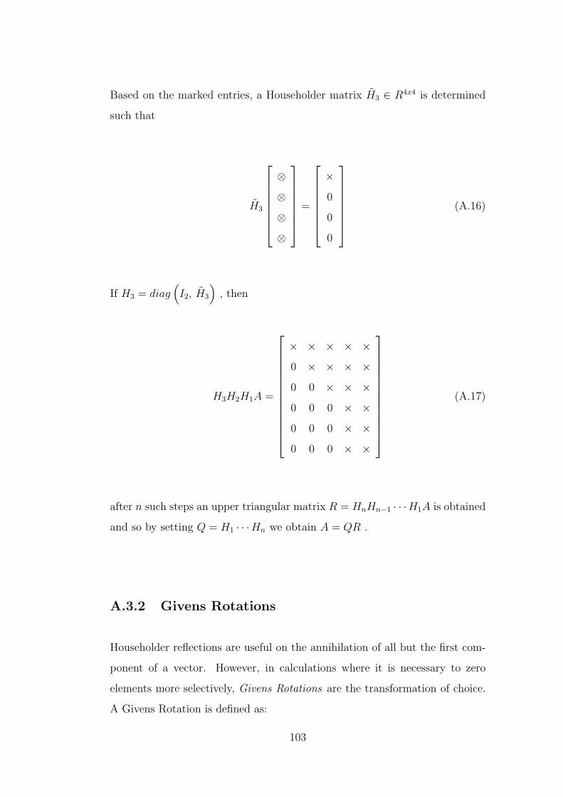
Based on the marked entries, a Householder matrix H3 ∈ R4x4 is determined

such that

H3

⊗⊗⊗⊗

=

×0

0

0

(A.16)

If H3 = diag(I2, H3

), then

H3H2H1A =

× × × × ×0 × × × ×0 0 × × ×0 0 0 × ×0 0 0 × ×0 0 0 × ×

(A.17)

after n such steps an upper triangular matrix R = HnHn−1 · · ·H1A is obtained

and so by setting Q = H1 · · ·Hn we obtain A = QR .

A.3.2 Givens Rotations

Householder reflections are useful on the annihilation of all but the first com-

ponent of a vector. However, in calculations where it is necessary to zero

elements more selectively, Givens Rotations are the transformation of choice.

A Givens Rotation is defined as:

103

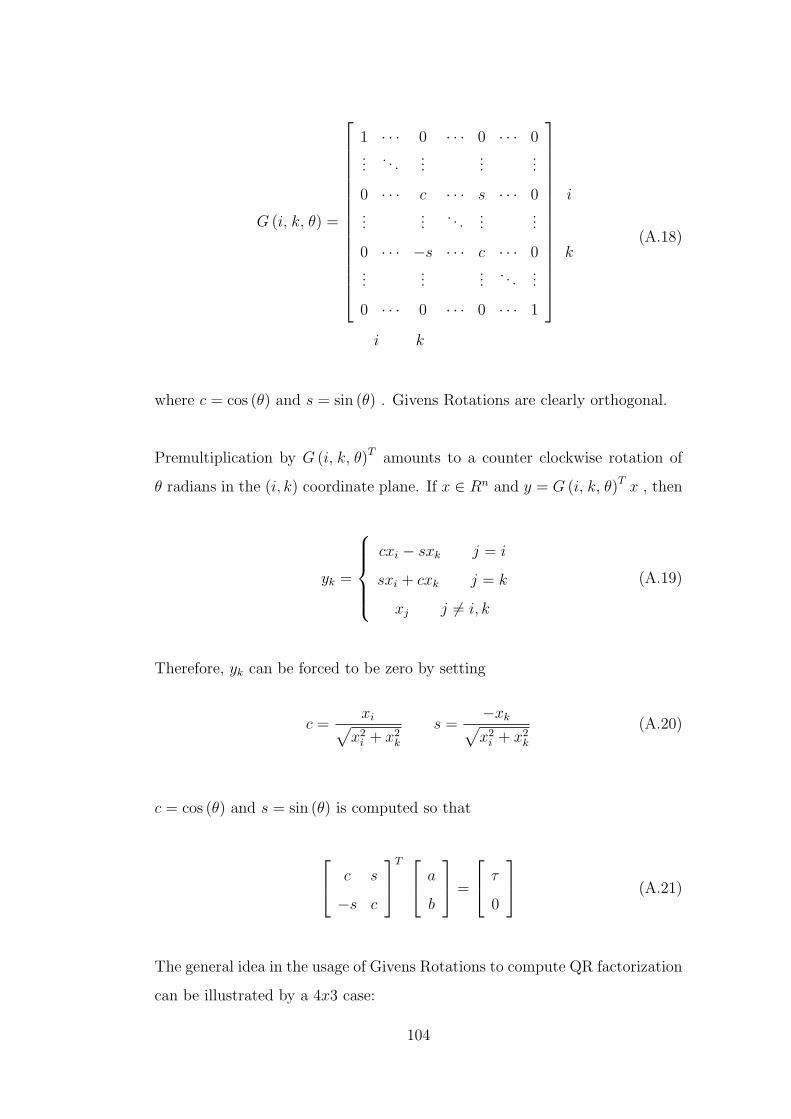
G (i, k, θ) =

1 · · · 0 · · · 0 · · · 0...

. . ....

......

0 · · · c · · · s · · · 0...

.... . .

......

0 · · · −s · · · c · · · 0...

......

. . ....

0 · · · 0 · · · 0 · · · 1

i

k

i k

(A.18)

where c = cos (θ) and s = sin (θ) . Givens Rotations are clearly orthogonal.

Premultiplication by G (i, k, θ)T amounts to a counter clockwise rotation of

θ radians in the (i, k) coordinate plane. If x ∈ Rn and y = G (i, k, θ)T x , then

yk =

cxi − sxk j = i

sxi + cxk j = k

xj j 6= i, k

(A.19)

Therefore, yk can be forced to be zero by setting

c =xi√

x2i + x2

k

s =−xk√x2

i + x2k

(A.20)

c = cos (θ) and s = sin (θ) is computed so that

c s

−s c

T a

b

=

τ

0

(A.21)

The general idea in the usage of Givens Rotations to compute QR factorization

can be illustrated by a 4x3 case:

104

× × ×× × ×× × ×× × ×

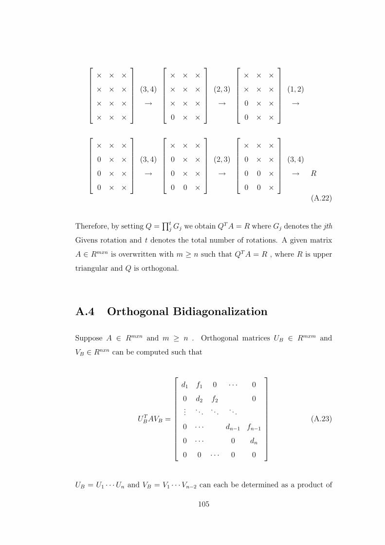
(3, 4)

→

× × ×× × ×× × ×0 × ×

(2, 3)

→

× × ×× × ×0 × ×0 × ×

(1, 2)

→

× × ×0 × ×0 × ×0 × ×

(3, 4)

→

× × ×0 × ×0 × ×0 0 ×

(2, 3)

→

× × ×0 × ×0 0 ×0 0 ×

(3, 4)

→ R

(A.22)

Therefore, by setting Q =∏t

j Gj we obtain QT A = R where Gj denotes the jth

Givens rotation and t denotes the total number of rotations. A given matrix

A ∈ Rmxn is overwritten with m ≥ n such that QT A = R , where R is upper

triangular and Q is orthogonal.

A.4 Orthogonal Bidiagonalization

Suppose A ∈ Rmxn and m ≥ n . Orthogonal matrices UB ∈ Rmxm and

VB ∈ Rnxn can be computed such that

UTBAVB =

d1 f1 0 · · · 0

0 d2 f2 0...

. . . . . . . . .

0 · · · dn−1 fn−1

0 · · · 0 dn

0 0 · · · 0 0

(A.23)

UB = U1 · · ·Un and VB = V1 · · ·Vn−2 can each be determined as a product of

105

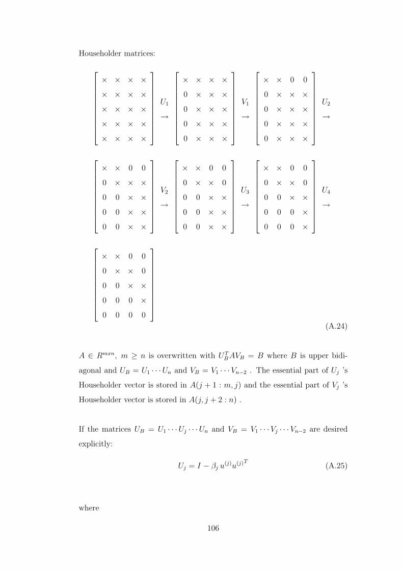
Householder matrices:

× × × ×× × × ×× × × ×× × × ×× × × ×

U1

→

× × × ×0 × × ×0 × × ×0 × × ×0 × × ×

V1

→

× × 0 0

0 × × ×0 × × ×0 × × ×0 × × ×

U2

→

× × 0 0

0 × × ×0 0 × ×0 0 × ×0 0 × ×

V2

→

× × 0 0

0 × × 0

0 0 × ×0 0 × ×0 0 × ×

U3

→

× × 0 0

0 × × 0

0 0 × ×0 0 0 ×0 0 0 ×

U4

→

× × 0 0

0 × × 0

0 0 × ×0 0 0 ×0 0 0 0

(A.24)

A ∈ Rmxn, m ≥ n is overwritten with UTBAVB = B where B is upper bidi-

agonal and UB = U1 · · ·Un and VB = V1 · · ·Vn−2 . The essential part of Uj ’s

Householder vector is stored in A(j + 1 : m, j) and the essential part of Vj ’s

Householder vector is stored in A(j, j + 2 : n) .

If the matrices UB = U1 · · ·Uj · · ·Un and VB = V1 · · ·Vj · · ·Vn−2 are desired

explicitly:

Uj = I − βj u(j)u(j)T (A.25)

where

106

u(j) =

0 0 · · · 0︸︷︷︸

j−1

1 u(j)j+1 · · · u(j+1)

m︸︷︷︸essential part

(A.26)

and

Vj = I − βj v(j)v(j)T (A.27)

where

v(j) =

0 0 · · · 0︸︷︷︸

j

1 v(j)j+2 · · · v(j+1)

n︸︷︷︸essential part

(A.28)

A.5 Direct Regularization Techniques

A.5.1 Tikhonov Regulatization

The key idea in Tikhonov’s method is to incorporate a priori assumptions

about the size and the smoothness of the desired solution, in the form of

the smoothing semi norm ‖Lx‖2 . For discrete ill-posed problems, Tikhonov

Regularization in general form leads to the minimization problem:

min ‖Ax− b‖2

2 + λ2 ‖Lx‖22

(A.29)

where the regularization parameter λ controls the weight given to minimization

of the regularization term, relative to the minimization of the residual norm.

Underlying this formulation, is the assumption that the errors in the right

hand side are uncorrelated and with covariance matrix σ20Im . If the covariance

matrix is of general form CCT , where C has full rank m, then one should scale

the least squares residual with C−1 and solve the scaled problem

107

min ∥∥ C−1 (Ax− b)

∥∥2

2+ λ2 ‖Lx ‖2

2

(A.30)

The Tikhonov problem has two important alternative formulations:

(AT A + λ2LT L

)x = AT b and min

∥∥∥∥∥∥

A

λL

x−

b

0

∥∥∥∥∥∥2

(A.31)

The Tikhonov solution xL,λ is given by

xL,λ = A#λ b with A#

λ =(AT A + λ2LT L

)−1AT (A.32)

where A#λ is the Tikhonov regularized inverse. If we insert GSVD of (A,L) into

this equation, then the filter factors for Tikhonov regularization in standard

form where L = In and general form where L 6= In are given by

fi =σ2

i

σ2i + λ2

, L = In and fi =γ2

i

γ2i + λ2

L 6= In (A.33)

For a square invertible L , the alternative formula

xL,λ =(LT L

)−1AT

(A

(LT L

)−1AT + λ2Im

)−1

b (A.34)

occasionally appears in literature.

The method also appears when the least squares problem is augmented with

statistical a priori information about the solution, in the form of a covariance

matrix CTx Cx for the desired solution (considered as a stochastic variable). In

this setting, the estimator is the solution to

108

(AT

(CCT

)−1A + (CxC)−1

)x = AT

(CCT

)−1b (A.35)

It can be seen that the estimator is the scaled Tikhonov solution when λL

is replaced by C−1x . In order to solve the Tikhonov problem numerically we

should form the matrix(AT A + λ2LT L

)and compute its Cholesky factoriza-

tion [46]. However, forming AT A explicitly can lead to loss of information

in finite-precision arithmetic and a new Cholesky factorization is required for

each regularization parameter λ .

Elden’s Bidiagonalization Algorithm is the most efficient and numerically sta-

ble way to compute the solution to the Tikhonov problem [3]. If the problem

is given in the general form (L 6= In) , then the standard forms of the matri-

ces A and b should be computed using explicit standard-form transformation

developed by Elden, which is based on two QR factorizations.

LT = KR =(

Kp Kn−p

) Rp

0

(A.36)

AKn−p = HT =(

Hn−p Hm−(n−p)

) Tn−p

0

(A.37)

Hence, the standard forms of the matrices A and b are obtained as

A = A(Ip −Kn−pT

−1n−pH

−1n−pA

)L+ (A.38)

=(Im −Hn−pH

Tn−p

)AL+

= Hm−(n−p)HTm−(n−p)AL+

b = b− AKn−pT−1n−pH

Tn−pb (A.39)

=(Im −Hn−pH

Tn−p

)b = Hm−(n−p)H

Tm−(n−p)b

where L+ = KpR−1p is the pseudo inverse of the full rank matrix L . Then

109

Tikhonov problem should be treated as a least squares problem of the form

min

∥∥∥∥∥∥

A

λIp

x−

b

0

∥∥∥∥∥∥2

(A.40)

This problem can be reduced to an equivalent sparse and highly structured

problem by transforming A into a pxp upper triangular matrix B by means of

left and right orthogonal transformations,

A = U B V T (A.41)

Once A has been reduced to a bidiagonal matrix B , we make the substitution

x = V ξ and obtain the problem:

min

∥∥∥∥∥∥

B

λLp

ξ −

UT b

0

∥∥∥∥∥∥2

(A.42)

The sub-matrix λLp can be annihilated by Givens Rotations as explained in

3.1.1. After λLp has been removed we arrive at the problem:

min

∥∥∥∥∥∥

B

0

ξ −

β1

β2

∥∥∥∥∥∥2

(A.43)

based on the fact that ‖Ax− b ‖22 =

∥∥ QT Ax−QT b∥∥2

2[49]. As a result, the

solution becomes:

ξ = B−1β1 (A.44)

We can also incorporate an a priori estimated x∗ into the smoothing norm and

thus “bias” the regularized solution towards this estimate. The least squares

estimation takes the form

110

min

∥∥∥∥∥∥

A

λL

x−

b

λLx∗

∥∥∥∥∥∥2

(A.45)

and after standard form transformation we have

min

∥∥∥∥∥∥

A

λIp

x−

b

λx∗

∥∥∥∥∥∥2

(A.46)

A.5.1.1 Least Squares with a Quadratic Constraint

There are two other regularization methods which are almost equivalent to

Tikhonov’s method, and which can be treated numerically by standard form

transformation plus bidiagonalization or GSVD. These two methods are for-

mulated as the following least squares problems with a quadratic constraint.

min ‖Ax− b‖2 subject to ‖L (x− x∗)‖2 ≤ α, (A.47)

min ‖L (x− x∗)‖2 subject to ‖Ax− b‖2 ≤ δ (A.48)

where α and δ are nonzero parameters each playing the role of the regular-

ization parameters. The solution to both problems is identical to xL,λ from

Tikhonov’s method. Graphically, the solution to A.25 lies on the intersection

of the Tikhonov L-curve and the horizontal line ‖L (x− x∗)‖2 = α , while the

solution to A.26 lies on the intersection of the L-curve and the vertical line

‖Ax− b‖2 = δ.

A.5.1.2 Inequality or Equality Constraints

It is sometimes convenient to add certain contraints to the Tikhonov solution,

such as nonnegativity, monotonicity, or convexity. All three constraints can be

111

formulated as inequality constraints of the form Gx ≥ 0 , taking the special

forms

x ≥ 0 nonnegativity

L1x ≥ 0 monotonicity

L2x ≥ 0 convexity

(A.49)

where L1 and L2 approximate the first and second derivative operators, re-

spectively [42]. The constraints can, of course, also be combined in the matrix

G. Thus, the inequality-constrained Tikhonov solution solves the problem

min ‖Ax− b‖2

2 + λ2 ‖Lx‖22

subject to Gx ≥ 0 (A.50)

The constraints can be in the form of equalities incorporated with total least

squares problems [42]. The general form of the linearly restricted least squares

problem is

min ‖Ax− b ‖2 such that Rx = r (A.51)

where R ∈ Rpxn . In order to solve the problem, method of Lagrangian multi-

pliers is used. The solution is found by minimizing the unconstrained problem

‖Ax− b‖2 − 2λ (Rx− r) (A.52)

with respect to x and λ = (λ1, . . . , λp) respectively and the following stationary

conditions are obtained:

2AT (Ax− b)− 2RT λ = 0 (A.53)

Rx− r = 0 (A.54)

112

Let S = AT A . From the first equation above,

x = S−1AT b + S−1RT λ = xols + S−1RT λ (A.55)

where xols = S−1AT b is the ordinary least squares solution under no restric-

tions. Multiplying by R and using the second equation:

Rxols + RS−1RT λ = Rx = r (A.56)

The symmetric RS−1RT is positive definite, hence invertible, and it is found

that

λ =[RS−1RT

]−1(r −Rxols) (A.57)

Inserting this into A.31 yields the solution

x = xols + S−1RT[RS−1RT

]−1(r −Rxols) (A.58)

A.5.1.3 Related Methods

The Tikhonov solution can be modified by a process which resembles iterative

refinement for linear systems of equations. If the set x(1) = xL,λ , then the

modified Tikhonov solutions are defined recursively as

x(k+1) = x(k)+(AT A + λ2LT L

)−1AT

(b− Ax(k)

), k = 1, 2, . . . (A.59)

This technique is called Iterated Tikhonov Regularization [46].

113

Another modification of Tikhonov’s method for achieving sharper filter fac-

tors amounts to solve the following system of equations in the standard form

case:

(AT A + λ2In + λ2

(AT A + λ2In

)−1)

x = AT b (A.60)

The corresponding filter factors are:

fi =σ2

i

σ2i + λ2 + λ2

/(σ2i + λ2)

(A.61)

For symmetric positive definite matrices A and L , Tikhonov’s problem is

suggested to be replaced with the problem:

(A + λL) x = b, λ ≥ 0 (A.62)

If L = In then the solution can be expressed in terms of the SVD of A, in

the form with filter factors fi = σi

σi+λ. If L 6= In then the solution is most

conveniently expressed in terms of the generalized eigenvalues and eigenvectors

of (A,L) .

Another variant of Tikhonov regularization is a statistical approach such that

the expected value ε(‖xexact − xreg‖2

2

)of the error norm is minimized. It is

assumed that b = bexact + e, xreg = A#b , and that the covariance matrix for

e is CCT . Then we obtain

ε(∥∥xexact − xreg

∥∥2

2

)=

∥∥xexact − A#bexact∥∥2

2+ trace

(A#CCT

(A#

)T)

=n∑

i=1

(1− fi)2 (

vTi xexact

)2+

n∑i=1

f 2i σ−2

i

∥∥CT ui

∥∥2

2

(A.63)

114

and this quantity is minimized for

fi =σ2

i

σ2i + ‖CT ui‖2

2

/(vT

i xexact)2, i = 1, . . . , n (A.64)

A.5.2 The Regularized General Gauss-Markov Linear

Model

The general Gauss-Markov linear model is defined as

Ax + ε = b (62) (A.65)

where A ∈ Rmxn (m ≥ n) and b ∈ Rm are known, x ∈ Rn is an unknown

vector to be estimated, and ε ∈ Rm is a random vector with zero mean and

variance-covariance matrix V (ε) = s2CCT with C ∈ Rmxq (m ≥ q) [50]. The

best linear unbiased estimator of x in this model is the solution to the problem:

min ‖u ‖2 subject to Ax + Cu = b (A.66)

where u ∈ Rq such that ε = Cu and u has the variance-coariance matrix

V (u) = s2Iq

When A is ill-conditioned while B is well-conditioned, a regularized Gauss-

Markov problem can be proposed as:

min‖u ‖2

2 + λ2 ‖Lx ‖22

subject to Ax + Cu = b (A.67)

This equation involves three matrices A, C and L where A ∈ Rmxn , C ∈ Rmxq

and L ∈ Rpxn . The appropriate tool for this analysis is the restricted SVD

(RSVD) where it is assumed that

115

rank (C) = q ≤ m,

rank (L) = p ≤ n ≤ m,

rank

A

L

= n.

(A.68)

Then, there exist nonsingular matrices X ∈ Rnxn and Z ∈ Rmxm , and orthog-

onal matrices U ∈ Rqxq and V ∈ Rpxp such that

ZT AX = Σ, ZT CU = M, V T LX = N, (A.69)

where Σ , N and M are pseudo diagonal matrices with nonnegative elements

having the following structure:

Σ =

ΣA 0 0 0

0 Ij 0 0

0 0 Ik 0

0 0 0 Il

0 0 0 0

s

j

k

l

u

(66.1)

t j k l

(A.70)

M =

Is 0

0 0

0 Ik

0 0

0 0

s

j

k

l

u

s k

N =

It 0 0 0

0 Ij 0 0

t

j

t j k l

(A.71)

116

and where

ΣA = diag(σ1, . . . , σmin(s,t)

) ∈ Rsxt, σ1 ≥ · · · ≥ σmin(s,t) > 0

j = rank (A, C) , k = n + q − rank

A C

L 0

,

l = rank

A C

L 0

− p− q, s = rank

A C

L 0

− n

t = ank (A, C)− rank

A C

L 0

, u = m− rank (A, C)

(A.72)

As a result, the solution xL,C,λ can be written as

xL,C,λ = XFλΣ+XT b, Fλ = diag (f1, . . . , ft, 1, . . . , 1) (A.73)

where

fi =σ2

i

σ2i + λ2

, i = 1, . . . , t (A.74)

As in the case of Tikhonov regularization, it is seen that λ controls the solu-

tion’s sensitivity to errors in b .

A.5.2.1 Numerical Algorithm

Equation A.67 can be reformulated as:

min

∥∥∥∥∥∥

λL 0

0 Iq

x

u

∥∥∥∥∥∥subject to

[A C

] x

u

= b (A.75)

117

A.5.2.1.1 Step1

Make a QR decomposition of C, so that C = Q

C1

0

, where C1 ∈ Rqxq

is upper triangular and nonsingular.

A.5.2.1.2 Step2

Let

QT [A b] =

A1 b1

A2 b2

q

m− q(A.76)

and make the following decomposition of A2 :

A2U = [ 0 A22] m− q (70)

n− i i(A.77)

so that U is orthogonal and A22 ∈ R(m−q)xi is of full column rank i.

A.5.2.1.3 Step3

Let

A1

L

U =

A11 A12

L1 L2

and UT x =

x1

x2

n− i

i

n− i i

(A.78)

Make a QR decomposition of A22 , so that A22 = Q1

A22

0

, where A22 ∈

Rixi is upper triangular and nonsingular. Let

QT1 b2 =

b

(1)2

b(2)2

with b

(1)2 ∈ Ri (A.79)

118

Then the regularized Gauss-Markov linear model is consistent only if b(2)2 = 0

[50]. In this case,

x2 = A−122 b

(1)2 (A.80)

and x1 solves the least squares problem:

min

∥∥∥∥∥∥

λL1

C−11 A11

x1 −

λL2x2

C−11 (b1 − A12x2)

∥∥∥∥∥∥(A.81)

This problem can be solved for x1 using plane rotations and orthogonal trans-

formations [50],[51] giving the unique solution:

x = U

x1

x2

(A.82)

A.5.3 Truncated SVD and GSVD (TSVD and TGSVD)

A different way to treat the ill-conditioning of A is to derive a new problem

with a well-conditioned rank-deficient coefficient matrix. This is the idea be-

hind the methods TSVD and TGSVD.

For problems with ill-determined numerical rank, it is not obvious that trun-

cation of the SVD/GSVD leads to regularized solution. However, it is proven

that under suitable conditions, for any valid truncation parameter k there al-

ways exists a regularization parameter λ such that TSVD/GTSVD solution is

close to Tikhonov solution.

119

The filter factors for these methods simply consist of zeros and ones:

TSV D : fi =

1, i ≤ k,

0, i > k

TGSV D : fi =

0, i ≤ n− k,

1, i > n− k

(A.83)

A.5.4 Algorithms based on Total Least Squares

In order to explain the basic idea behind this method, consider a moment

the usual least squares solution xols found by minimizing ‖Ax− b‖2 . It can

be seen that xols solves the problem Ax = b where b is the smallest possible

perturbation if b such that b ∈ < (A) , i.e, such that∥∥∥b− b

∥∥∥ is minimal.

In other words, we first perturb b just enough to ensure that the perturbed

equation has a solution, and then xols is found solving this system. If A is

also subject to noise, A can be perturbed as well as b . That is, we can try to

find A and b such that∥∥∥[A; b]−

[A; b

] ∥∥∥ is as small as possible and such that

b ∈ <(A

). Then Ax = b has a solution, and any such solution is called total

least squares (TLS) solution of the problem Ax = b .

A.5.4.1 Truncated Total Least Squares (TTLS)

TTLS is a modification of TLS, which is also suitable as a regularization

method for ill-posed problems. The TTLS solution is usually defined as fol-

lows:

Suppose a regularization parameter k has been specified and consider the sin-

gular value decomposition

[A b] = UDV T (A.84)

where V ∈ R(n+1)x(n+1) can be block partitioned as

120

V =

V11 V12

V21 V22

(A.85)

where V11 ∈ Rnxk . Then the TTLS solution is defined by

xttls = − V12VT22∥∥∥V22

∥∥∥2

2

(A.86)

and the filter factors corresponding to uTi 6= 0 and σi 6= 0 are given by

fi =k∑

j=1

v2n+1,j∥∥∥ V22

∥∥∥2

2

(σ2

i

σ2j − σ2

i

)(A.87)

For i ≤ k , these filter factors increase monotonically with i and satisfy

0 ≤ fi − 1 ≤ σ2k+1

σ2i − σ2

k+1

, i ≤ k, (A.88)

while for k < i < rank (A) , these filter factors satisfy

0 ≤ fi ≤∥∥∥ V22

∥∥∥−2

2

σ2i

σ2k − σ2

i

, k < i < rank (A) (A.89)

It can be observed that for the first k filter factors, the larger the ratio between

σi and σk+1 , the closer the bound on fi to 1 . Similarly, for the last n − k

filter factors, it is observed that the smaller the ratio between σi and σk , the

closer fi is toσ2

i

σ2k

.

A.5.4.2 Regularized TLS (R-TLS)

An alternative approach to adding regularization to the TLS technique is based

on Tikhonov formulation (*). In the TLS setting we add the bound ‖Lx ‖2 ≤α to the ordinary TLS problem and the R-TLS problem thus becomes,

121

min∥∥∥ (A, b)−

(A, b

) ∥∥∥F

subject to b = Ax, ‖ L x ‖2 ≤ α.

(A.90)

The R-TLS solution xα to A.55 is a solution to the problem

(AT A + λIIn + λLLT L

)x = AT b (A.91)

where the parameters λI and λL are given by

λI = −‖Ax−b ‖221+‖x ‖22

,

λL = (b−Ax)T Axα2

(A.92)

Moreover, the TLS residual satisfies,

∥∥∥ (A, b)−(A, b

) ∥∥∥2

F= −λI (A.93)

The expressions for the parameters λI , λL and the residual are proven us-

ing Lagrange multiplier formulation in [52]. In the standard form case, the

Tikhonov problem becomes

min ‖ Ax− b ‖F subject to ‖ x ‖2 ≤ α. (A.94)

with solution xα satisfying

(AT A + λIn

)xα = AT b (A.95)

Similarly, R-TLS problem takes the form,

min∥∥∥ (A, b)−

(A, b

) ∥∥∥F

subject to b = Ax, ‖ x ‖2 ≤ α.

(A.96)

122

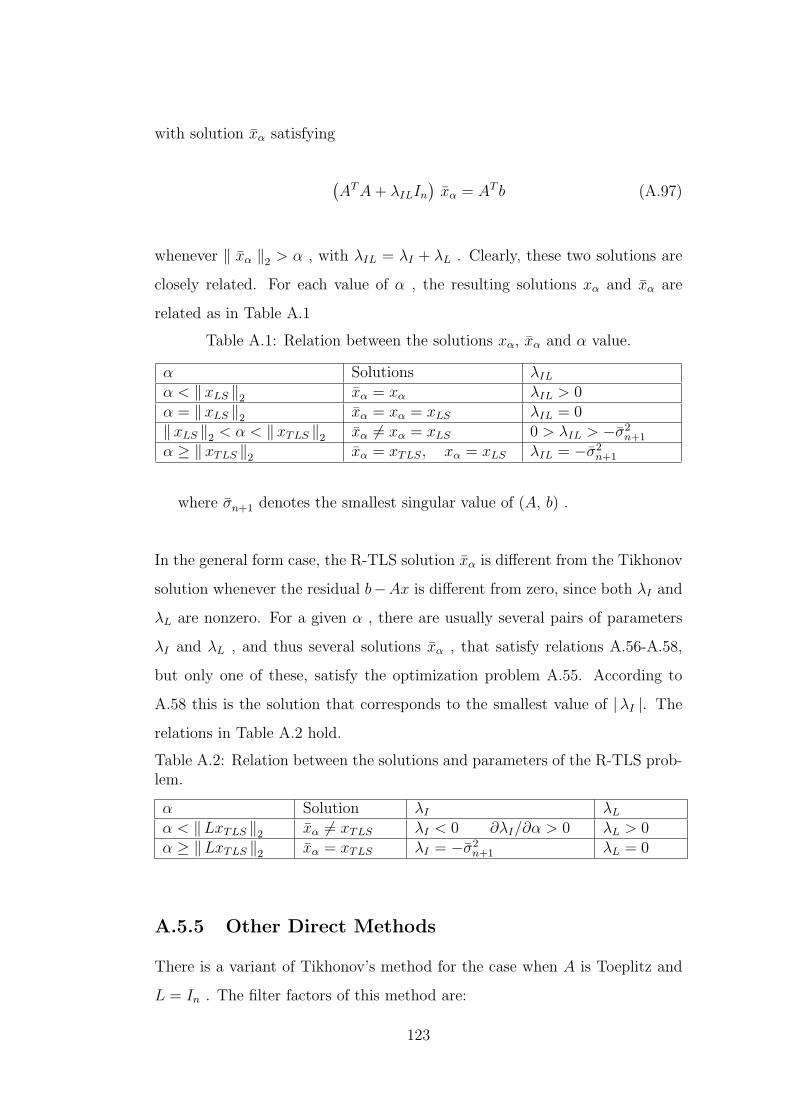
with solution xα satisfying

(AT A + λILIn

)xα = AT b (A.97)

whenever ‖ xα ‖2 > α , with λIL = λI + λL . Clearly, these two solutions are

closely related. For each value of α , the resulting solutions xα and xα are

related as in Table A.1

Table A.1: Relation between the solutions xα, xα and α value.

α Solutions λIL

α < ‖ xLS ‖2 xα = xα λIL > 0α = ‖ xLS ‖2 xα = xα = xLS λIL = 0‖xLS ‖2 < α < ‖xTLS ‖2 xα 6= xα = xLS 0 > λIL > −σ2

n+1

α ≥ ‖ xTLS ‖2 xα = xTLS, xα = xLS λIL = −σ2n+1

where σn+1 denotes the smallest singular value of (A, b) .

In the general form case, the R-TLS solution xα is different from the Tikhonov

solution whenever the residual b−Ax is different from zero, since both λI and

λL are nonzero. For a given α , there are usually several pairs of parameters

λI and λL , and thus several solutions xα , that satisfy relations A.56-A.58,

but only one of these, satisfy the optimization problem A.55. According to

A.58 this is the solution that corresponds to the smallest value of |λI |. The

relations in Table A.2 hold.

Table A.2: Relation between the solutions and parameters of the R-TLS prob-lem.

α Solution λI λL

α < ‖LxTLS ‖2 xα 6= xTLS λI < 0 ∂λI/∂α > 0 λL > 0α ≥ ‖LxTLS ‖2 xα = xTLS λI = −σ2

n+1 λL = 0

A.5.5 Other Direct Methods

There is a variant of Tikhonov’s method for the case when A is Toeplitz and

L = In . The filter factors of this method are:

123

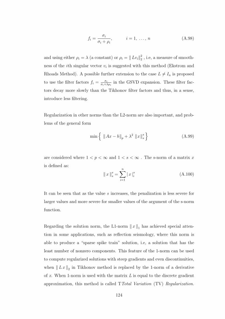
fi =σi

σi + ρi

, i = 1, . . . , n (A.98)

and using either ρi = λ (a constant) or ρi = ‖Lvi‖22 , i.e, a measure of smooth-

ness of the ith singular vector vi is suggested with this method (Ekstrom and

Rhoads Method). A possible further extension to the case L 6= In is proposed

to use the filter factors fi = σi

σi+λµiin the GSVD expansion. These filter fac-

tors decay more slowly than the Tikhonov filter factors and thus, in a sense,

introduce less filtering.

Regularization in other norms than the L2-norm are also important, and prob-

lems of the general form

min‖Ax− b‖p + λ2 ‖x‖s

s

(A.99)

are considered where 1 < p < ∞ and 1 < s < ∞ . The s-norm of a matrix x

is defined as:

‖x ‖ss =

n∑i=1

| x |si (A.100)

It can be seen that as the value s increases, the penalization is less severe for

larger values and more severe for smaller values of the argument of the s-norm

function.

Regarding the solution norm, the L1-norm ‖x ‖1 has achieved special atten-

tion in some applications, such as reflection seismology, where this norm is

able to produce a “sparse spike train” solution, i.e, a solution that has the

least number of nonzero components. This feature of the 1-norm can be used

to compute regularized solutions with steep gradients and even discontinuities,

when ‖Lx ‖2 in Tikhonov method is replaced by the 1-norm of a derivative

of x. When 1-norm is used with the matrix L is equal to the discrete gradient

approximation, this method is called TTotal Variation (TV) Regularization.

124

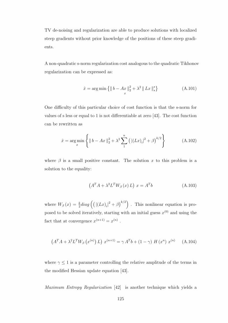
TV de-noising and regularization are able to produce solutions with localized

steep gradients without prior knowledge of the positions of these steep gradi-

ents.

A non-quadratic s-norm regularization cost analogous to the quadratic Tikhonov

regularization can be expressed as:

x = arg min‖ b− Ax ‖2

2 + λ2 ‖Lx ‖ss

x

(A.101)

One difficulty of this particular choice of cost function is that the s-norm for

values of s less or equal to 1 is not differentiable at zero [43]. The cost function

can be rewritten as

x = arg minx

‖ b− Ax ‖2

2 + λ2

n∑1

( |(Lx)i|2 + β)k/2

(A.102)

where β is a small positive constant. The solution x to this problem is a

solution to the equality:

(AT A + λ2LT Wβ (x) L

)x = AT b (A.103)

where Wβ (x) = k2diag

(( |(Lx)i|2 + β)k/2

). This nonlinear equation is pro-

posed to be solved iteratively, starting with an initial guess x(0) and using the

fact that at convergence x(n+1) = x(n) .

(AT A + λ2LT Wβ

(x(n)

)L

)x(n+1) = γ AT b + (1− γ) H (xn) x(n) (A.104)

where γ ≤ 1 is a parameter controlling the relative amplitude of the terms in

the modified Hessian update equation [43].

Maximum Entropy Regularization [42] is another technique which yields a

125

solution with only positive elements. The solution is defined much the same as

the Tikhonov regularization, the only difference being the choice of the penalty

term such that:

xme = arg minx

‖ b− Ax ‖2

2 + λ2

n∑1

xi log (wixi)

, xi ≥ 0 (A.105)

where wi are positive weights. It can be observed that the maximum entropy

method penalizes large elements xi less than Tikhonov regularization method

as illustrated in Figure A.1.

Figure A.1: Penalty term comparison

Note that the maximum entropy penalty is minimized when the ith component

of x is equal to x∗i = e−1/wi

wi(assuming log is the natural logarithm). Selecting

all wi equal, we implicitly penalize for large differences in values between the

components of x. The latter effect could also have been obtained by a Tikhonov

penalty of the form ‖ x− x∗‖ , where x∗ is a vector with all components equal.

126

A.6 Iterative Regularization Methods

Iterative methods for linear systems of equations ad linear least squares prob-

lems are based on iteration schemes that access the coefficient matrix A only

via matrix-vector multiplications with A and AT , and they produce a sequence

of iteration vectors x(k), k = 1, 2, . . . , that converge to the desired solution.

Iterative methods are preferable to direct methods when the coefficient matrix

is so large that it is too time-consuming or too memory demanding to work

with an explicit decomposition of A [46].

A.6.1 Landweber Iteration

This is one of the main iterative regularization methods, which takes the form

x(k) = x(k−1) + wAT(b− Ax(n−1)

)(A.106)

where x(0) = 0 , w is a real parameter satisfying 0 < w < 2∥∥AT A

∥∥−1

2. After

k iterations, we have the filtering factors:

f(k)i = 1− (

1− wσ2i

)k, i = 1, . . . , n (A.107)

A disadvantage of this method is that it may take many steps k to achieve a

useful regularized solution [42].

A.6.2 Regularizing Conjugate Gradient(CG) Iterations

The CG method was originally developed for solving large sparse systems of

equations with a symmetric positive definite coefficient matrix. Applying the

method to normal equations AT Ax = AT b produces iterates which converges

to a least squares solution for the problem Ax = b . One implementation of the

CG method for solving the system AT Ax = AT b is the CGLS method which

iterates the following statements [42],[46] for k = 1, 2, . . . :

127

αk =‖AT r(k−1)‖2

2

‖Ad(k−1)‖2

2

x(k) = x(k−1) + αkd(k−1),

r(k) = r(k−1) − αkAd(k−1), (101)

βk =‖AT r(k)‖2

2

‖AT r(k−1)‖2

2

,

d(k) = AT r(k) − βkAd(k−1)

(A.108)

where r(k) is the residual vector r(k) = b − Ax(k) . The CGLS algorithm is

initialized by with the starting vector x(0) = 0 , r(0) = b and d(0) = AT r(0) .

It can be observed that the CG method avoids the computation of AT A ,

which is numerically an advantage as AT A is worse conditioned than A and

AT . The filter factors for the CG method after k iterations can be shown to

be:

f(k)i = 1−

k∏j=1

θ(k)j − σ2

i

θ(k)j

, i = 1, . . . , n (A.109)

where θ(k)1 ≥ θ

(k)2 ≥ · · · ≥ θ

(k)k are called Ritz values [42]. The Ritz values

can be precisely defined and can be shown to approach squared singular values

such that θ(k)j → σ2

j as k → n where k ≤ n . Also, A.109 requires that

f(k)i = f

(k)j whenever σi = σj . Furthermore, we have f

(k)i → 1 as k → n

, which states the fact that CG iterates converge towards the least squares

solution.

128

rf coil system design for mri applications in ...teorik olarak hesaplanan manyetik alan ile...

Documents