Road Flooding in Coastal Connecticut: Final Report to South Central Regional Council of Governments

James O’Donnell,1,2 Kay Howard Strobel2, Michael Whitney2,

Alejandro Cifuentes-Lorenzen2 and Todd Fake2

1Connecticut Institute for Resilience and Climate Adaptation 2Department of Marine Sciences

The University of Connecticut

June 30, 2017

      

Executive Summary

The towns of Branford and Guilford are concerned about flooding and access on Route 146 in both towns. The proximity to tidal wetlands and the minimal elevation difference above tidal wetlands in many areas makes the roadway extremely vulnerable to tidal flooding, both now and as sea level gradually increases. The study provides information on current and potential impacts. This information can be used as a basis for addressing access during normal tidal cycles and storm events, future resiliency measures and future roadway improvements.

We have performed extensive measurements of water level fluctuation and road elevations in areas that were identified as prone to coastal flooding. We integrated these measurements using mathematical models as statistics to characterize the current risk more quantitatively, and to assess the impact of rising sea levels.

Sachems Head Road (RT 146) in Guilford floods when the water in The Cove exceeds 1.1 m (NAVD88). The frequency of flooding is effectively controlled at the moment by the presence of the berm that carries Daniel Avenue and the flow restriction to the marsh imposed by the size of the culvert. Since the elevation of Daniel’s Avenue is only 1.5 m, NAVD 88, severe storms can lead to flow over the road which reduces the flood protection value substantially. This has occurred twice since 1999. An increase in mean sea level of 0.25 m will lead to overtopping more frequently. A precise estimate of the risk would require more observations of the flow over the road, but yearly flooding is likely.

Leetes Island Road (RT 146) in Guilford passes through the northern edge of the marsh system that forms the Great Harbor Wildlife Area. Flooding has occurred in two areas. We measured the elevation of the relevant sections of road and found the lower levels to be at 1.1 m NAVD88. We examined topography of the region, and made water level measurements, and concluded that water from Long Island Sound influences the two eastern basins of the complex and controls flooding of the eastern section of Leetes Island Road. Simulations showed that the constriction in the width of the entrance to the marsh at Trolley Road substantially reduces the water level fluctuation at Leetes Island Road though flooding still occurs each year. Severe storms, like Hurricane Irene and super storm Sandy, cause flow over Trolley Road and extensive flooding at Leetes Island Road. A 0.25 m increase in mean sea level will increase the frequency of flooding substantially. The water level in the western basin fluctuates independently and determines the flooding risk in the western section. It is controlled by flow into the western basin at Shell Beach Road. Flooding is unlikely there unless severe storms drive water over the road. Sea level rise will not increase the flooding risk in western section of Leetes Island Road.

Indian Neck Avenue and RT146 in Branford both cross the Branford River on bridges and then pass through underpasses to reach the north side of the AMTRAK rail line. We measured the levels of the roads and the surrounding topography to determine the water level that will lead

to flooding of the two underpasses. We also deployed instruments to measure water level fluctuations and showed that the difference between the level at New Haven and the Bridges was minimal, thereby allowing the use of the long record there do assess flooding risk. The RT 146 underpass will flood when the level exceeds 1.6 m, which we expect to occur every year. The Indian Neck Avenue underpass floods when the water level exceeds 1.75 m which has a 25% probability per year. A 0.25 m increase in mean sea level will lead flooding multiple times per year in both locations.

Linden and Sybil Avenues in Branford are located to the east of the bridge and tide-gate structure that caries Sybil Avenue (RT 146) across Sybil Creek. We made elevation measurements that show the bridge and low areas of the Road are at 1.9 m NAVD88. We also made water level measurements that show the levels at Sybil Avenue vary in line with the measurements are the New Haven tide gage. Analysis of the highest water levels in New Haven show that the 1.9 m level was reached or exceeded 4 times since 1999. An increase of mean sea level of 0.25 m would cause the road level to be exceed by 20 storms. When the road level is exceeded, water can flow over the road and into the marsh surrounding Sybil Creek and cause flooding in the adjacent neighborhoods.

Limewood Avenue (RT 146) and Waverly Road, Branford, lie to the south and east of the bridge over Sybil Creek. A segment of Limewood Avenue follows the shore of Long Island Sound and during super storm Sandy wave over-topping was reported to have caused extensive flooding of Limewood Avenue, and the water then drained down Waverly Road to the Jarvis Creek marsh. We made elevation measurements to characterize the topography of the coastal area, and wave and water elevation measurements to evaluate the skill of models. We estimate the over-topping flux from Limewood Avenue and the flow over Sybil Creek Avenue into the marsh and find that the predicted high water level in the marsh was similar to that observed by the USGS survey. Most of the water was a consequence of the wave driven flux. Even though the fluxes were high, the large area of the marsh was able to contain the volume below 1.1 m and flooding was avoided in many residences. At a 0.25 m higher mean sea level, simulation show that the flood protection value is much reduces and Sandy would cause flooding around the marsh to 1.9m. At current sea levels overtopping at Limewood is infrequent, however, risk estimation will require the development of a joint probability distribution of wave and water levels.

RT 146 at Jarvis Creek, Branford, experiences flooding at two locations, near the bridge over the creek, and to the east, at the underpass at the AMTRAK line. Measurement of the road elevation showed that both areas were at 1.1 m. The underpass is near an area of the marsh where the flow is unrestricted and water levels are essentially the same as at New Haven. Water level fluctuations at the bridge are reduced by a tide gate and berm in the marsh. We used a model to simulate the elevation at the marsh using the New Haven data to force the model. If tidal fluctuations alone are considered then the underpass should be expected to flood on 5 days per and 0.1 m increase in the mean sea level would double that. Currently no flooding would occur

at the bridge due to tides alone, and 0.20 m increase would be required to cause flooding on two days per year. Consideration of meteorological effects shows that at both locations, a 0.1 m increase in mean sea level will double the expected probability of a high water level that currently is the highest of the year.

1  

1. Introduction

The coastline of Connecticut is incised by numerous inlets where the streams and rivers carrying runoff from land towards the ocean and the saline tidal waters of Long Island Sound intrude into the channels. Salt marshes have formed in many of these inlets and have become critical habitat for numerous species of insects, birds and fish. Coastal settlements, and the routes between them, have general skirted the inland limits of the salt marshes and many bridges and culverts have been constructed to allow the water and transportation network to co-exists. Rising sea levels will cause segments of roadways to become more vulnerable to flooding in the future. Assessing the most cost effective and appropriate adaptation strategy to reduce the frequency of flooding to an acceptable level requires analysis of the flow of water through the inlets.

The South Central Regional Council of Governments (SCRCOG) and the towns of Branford and Guilford share concerns about persistent flooding of coastal roads and in this project we develop an approach to estimating the frequency of flooding at sites on RT 146 that allow the development and testing of approaches to evaluating adaptation options. The sites selected have contrasting geomorphology and hydrodynamic conditions and different approaches are used in each. The report will address each of the case study separately. Extensive details describing the data collection and model development activities that are common to the program are provided in Appendices.

The study areas in Guilford are (1) The Cove, and (2) Great Harbor Wildlife Area. Figure 1 shows a GoogleEarth map of the region. The green and blue arrows identify where there is concern about road flooding. Figure 2 shows a GoogleEarth map of the Branford study areas. Area (3), is centered at Indian Neck Avenue and RT 146 at the bridge across the Branford River. The location of flooding in study area (4) is indicated by the blue arrow at the junction of Linden and Sybil (RT 146) Avenues in Branford where a bridge crosses the marsh and a tide gate restricts the east-west flow of water. Wave splash-over at the shore in Area (5), near Limewood Avenue and Waverly Road, Branford, is examined. In an earlier study, (O’Donnell et al., 2016) the effect of a tide gate and berm on flooding at RT 146 near Jarvis Creek, Branford, was examined. Case study (6) will expand on the earlier study to characterize the statistics of flooding and the effect of sea level rise in this area.

Our basic approach is to develop relationships between the long term observations of sea level fluctuations at the NOAA tide gages in Long Island Sound and water levels at the study sites using a combination of observations and mathematical models that represent the flow of water through the channels and flow control structures that connect the sites and Long Island Sound. Since each site has important differences, we present the results at each area separately.

2  

 

Figure 1. The coastline of Guilford is shown using a GoogleEarth image with some locations of flooding on RT 146 indicated by the blue and green arrows. To understand how the water level in the Sound drives flooding we deployed instruments to measure sea level at the 5 locations shown red. 

 

Figure 2. The coastline of Branford is shown using a GoogleEarth image with some locations of flooding on RT 146 indicated by the blue and yellow arrows. To understand how the water level in the Sound drives flooding we deployed instruments to measure sea level at the 3 locations shown by the red diamonds. We also deployed a wave sensor at approximately the location of the yellow *. 

Area 1Area 2

Area 3

Area 4

Area 5*

3  

 

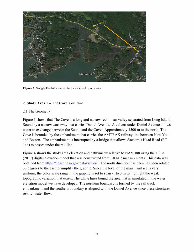
Figure 3. Google Earth© view of the Jarvis Creek Study area.

2. Study Area 1 – The Cove, Guilford.

2.1 The Geometry

Figure 1 shows that The Cove is a long and narrow rectilinear valley separated from Long Island Sound by a narrow causeway that carries Daniel Avenue. A culvert under Daniel Avenue allows water to exchange between the Sound and the Cove. Approximately 1500 m to the north, The Cove is bounded by the embankment that carries the AMTRAK railway line between New Yok and Boston. The embankment is interrupted by a bridge that allows Sachem’s Head Road (RT 146) to passes under the rail line.

Figure 4 shows the study area elevation and bathymetry relative to NAVD88 using the USGS (2017) digital elevation model that was constructed from LIDAR measurements. This data was obtained from https://coast.noaa.gov/dataviewer/. The north direction has been has been rotated 33 degrees to the east to simplify the graphic. Since the level of the marsh surface is very uniform, the color scale range in the graphic is set to span -1 to 3 m to highlight the weak topographic variation that exists. The white lines bound the area that is simulated in the water elevation model we have developed. The northern boundary is formed by the rail track embankment and the southern boundary is aligned with the Daniel Avenue since these structures restrict water flow.

Area 6

4  

 

Figure 4. Bathymetry and elevation (meters relative to NAVD88) in The Cove study area. The white rectangle identifies the area used in the evaluation of the basin area and volume. The horizontal coordinates are in meters.

Water from Long Island Sound enters The Cove through a culvert below Daniel Avenue. Figure 5(a) shows a higher resolution view of the south end of the cove using the topography shown in Figure 4. To establish the level of the road surface we performed a survey using an RTK GPS system which yields elevation measurements with a precision of 0.03 m. The numbered points indicate the location of the survey points. A detailed description of these measurements is provide in Appendix A. Figure 5(b) shows the levels obtained in the survey plotted with distance along the road from the south west (points 1 and 2). The highest points are on the bridge over the culvert where the road surface reaches 2m NAVD88. However, much of the road is below that level at approximately 1.5m.

Using additional survey points, the width and length of the culvert and entrances were estimated to be 2 m, and 20 m respectively. The height of the culvert is 1.7m and the bottom lies at NVGD88 level -0.3.

The area of primary concern for road flooding is located at the northern area of The Cove where Sachems Head Road (RT 146) passes under the rail line. Figure 6 (a) shows the locations of the elevation measurements as red dots with numbers so that the locations can be coordinated with the levels shown in Figure 6 (b). Note that the road crosses under the rail line between points 72 and 71. The elevation data (relative to NAVD88) are displayed in Figure 6 (b) as a function of distance along the road from the center of the underpass. Negative distance values indicate points to the south of the tracks where the level of the road drops from 1.24 m to 1.08 m. To the north of the track the level rises to 1.70 m and then drops back to 1.5 m.

5  

 

 

Figure 5. (a) The topography of the north end of The Cove. The red dots show locations on Sachems Head Road (RT 146) where the elevation measurements shown in Figure 6 were obtained. (b). Elevation measurements of the elevation of Sachems Head Road (RT 146) where it crosses under the AMTRAK line. The numbers indicate the locations shown in Figure 6(a). The horizontal axis shows the distance (in meters) from the bridge. Negative (positive) values are to the south (north) of the bridge.

 

Figure 6. (a) The topography of the south end of The Cove in the vicinity of Daniel Avenue. The red numbered dots show locations of the survey points. (b) Elevation measurements of at the locations shown in 6(a). The horizontal axis shows the distance (in meters) from the AMTRAK bridge. Negative (positive) values are to the south (north) of the bridge 

The model we present in the next section requires that we know how the area of the water surface in the basin (𝐴 ) varies with the level of the water (𝜂 . This is simply computed from the gridded LIDAR elevation data by counting the number of cells with level less than, or equal to, the level 𝜂 for values 𝜂 1, 0.9, 0.8, … 0.0, 0.1, 0.2, … 5.0 m. Figure 7(a) shows the area

6  

(horizontal axis) computed for each interval. The distribution is extremely peaked with the maximum, 55 10 m2 at the 0.4-0.5 interval which is the level of the marsh surface. The blue line in Figure 7 (b) shows the variation of the total area (horizontal axis) below the elevation shown on the vertical axis. Note the area is displayed on a logarithmic scale. The analysis shows that the area increases rapidly from 0.3 m elevation where it is 9 10 m2, to 0.6 m where it reaches 129 10 m2. It approximately doubles to 205 10 m2 at 1.3 m and then slowly increase to 228 10 m2 at 2 m. This steep sided channel geometry is characteristic of many tidal marsh systems in Connecticut and is a consequence of marsh migration into glacially eroded channels. 

 

Figure 7. (a) The horizontal axis shows the area of The Cove, defined in Figure 4, in 0.1 m elevation intervals. (b) The area of the domain below level shown on the vertical axis. Note that the elevations are relative to NAVD88 and the data USGS (2017) LIDAR-based bathy-topography.

2.2 Mathematical Model

The fundamental principle that we exploit to simulate the water level fluctuations follows the model proposed by Roman et al. (1995), which assumes that the rate of change of the volume of water in a basin, 𝑉 , with time, 𝑡, is equal to the rate at which it enters from the upland source (a small stream) minus the rate at which it exchanges with the Sound can be expressed mathematically as

𝑑𝑉𝑑𝑡

𝑄 𝑄 , ,

(1)

where the symbols 𝑄 and 𝑄 , represent the flow rates into, and out of, the basin. Note that

𝑉 depends upon the bathymetry of the basin and the water level 𝜂 . Since the water level in the

(a) (b) 

7  

Sound, 𝜂 , can be higher or lower than that in the estuary, 𝜂 , the flux 𝑄 , can be either positive

or negative. The well-established Manning Formula (Linsley and Franzini, 1979) is used to relate the flow rate to the sea level difference as

𝑄 ,

𝐴 ,

𝑛 , 𝑃 ,

|𝜂 𝜂 |

𝐿 ,

𝜂 𝜂|𝜂 𝜂 |

,

(2)

where 𝐴 , and 𝐿 , are the cross sectional area and length of the flow constriction, 𝑃 , is the

“wetted perimeter”, the length of the intersection between the water and rigid boundary in the cross-sectional plane. The friction parameter is 𝑛 , and is referred to as the Manning

coefficient. Note that the units of 𝑛 , (not usually reported in SI units) are s/m1/3. Values for a

variety of channel types have been estimated empirically and are reported in many text books (e.g. Chow, 1959). High values (approximately 0.1 s/m1/3) are found where there is vegetation and boulders in the flow and when the channel has abrupt variation. In this model the parameter includes the effects of flow in the marsh and we anticipate higher values than the normal range. We us 𝑛 , as a calibration parameter and estimate it by comparison of model solutions to

observations. Note that the sign of 𝑄 , is positive when 𝜂 𝜂 , i.e. the flow is out of the basin.

It is also important to note that the cross section and wetted perimeter vary with the water levels: i.e. 𝐴 , 𝐴 , 𝜂 , 𝜂 , and 𝑃 , 𝑃 , 𝜂 , 𝜂 .

The area, 𝐴 , 𝜂 , 𝜂 , and wetted perimeter, 𝑃 , 𝜂 , 𝜂 , parameters vary with the water levels

and these dependences, together with the constriction length, 𝐿 , , must be prescribed by

measurement. The Manning coefficients, 𝑛 , , can be estimated using literature values and

refined by a systematic calibration procedure which minimizes the differences between the measurements and predictions of 𝜂 𝑡 and 𝜂 𝑡 .

The complexity of the equations requires that numerical methods be employed. The differential equations were solved using the programming and computing environment MATLAB©. Changes in the basin areas with elevations were prescribed using an analysis of LIDAR elevation data (see section 2.3). The river source (𝑄 could be estimated using stream discharge and precipitation measurements, however, the fluxes are small and we omitted them in this study.

2.3 Observations

To develop optimal estimates of the parameters in Equation (2) and to assess the consistency of the model we deployed a water level sensors in The Cove at the locations labeled 4 and 5 in Figure 1. The details of the equipment and the deployment times and dates are provided in Appendix 2. Unfortunately, the sensors at Site 5 failed due to corrosion of the connectors.

The pressure sensor at site 4 was located on the sediment surface at longitude -72.6938154°, latitude 41.2683542° on the 13th of October, 2016. The level of the sensor was estimated form measurements with an RTKGPS system and sounding line as 0.05 m (NAVD88). It was recovered on 20 January, 2017. An earlier attempt to recover the instrument was unsuccessful

8  

because of extensive ice in The Cove. The instrument then was dragged off station before it could be recovered. Figures 8(a) and 8(b) a shows the temperature and water level observations. Note that the water level estimates from the pressure sensor were corrected for fluctuation in atmospheric pressure using an additional sensor deployed on land nearby (see Appendix 2). The weather during the observation period was not unusual for the late fall-early winter and a representative data set was acquired. To gather more data, we redeployed the equipment in April 17th and recovered it on June 21st, 2017.

The water level fluctuation outside of the basin in Long Island Sound are approximately the same as at the NOAA tide gage at New Haven (downloaded for the period of the instrument deployment from https://tidesandcurrents.noaa.gov/waterlevels.html?id=8465705) and the pressure sensor moored of Branford at the location shown by the yellow * in Figure 2. These are highly correlated, as is evident in Figure 9, which shows the New Haven observations (horizontal axis) and the level off Branford (vertical axis). A least-squares linear regression is shown by the green dashed line and has a slope of 0.92 suggesting that the amplitude of the fluctuations off Branford are approximately 8% less than at New Haven.

 

Figure 8. (a) The evolution of the water temperature (Celsius) measured at Station 4 in The Cove is shown by the black and red lines. The interval in red shows the measurements after the sensor was frozen. (b) The measurements of water level. Red shows where the data is unreliable.

The black line in Figure 10 shows the time history of the hourly observations at the NOAA tide gage in New Haven for the period of the instrument deployment. The water level estimated at Site 4 which are shown by the blue line. The longer term fluctuations in the Sound water level were extracted from the hourly measurements at New Haven and Branford using a 36 hour Hamming filter and these are shown in by the red and green lines in Figure 10. It is clear that there culvert at Daniel Avenue effectively reduces the amplitude of the tidal variation and limits

(b) 

(a) 

9  

the maximum elevation during the study interval to 0.65 m (NAVD). This level is sufficient to flood much of the surface of the marsh, see Figure 7(a).

 

 

Figure 9. The relationship between hourly water level (m) measurements at New Haven and that at Branford at the site shown by the yellow * in Figure 2. The slope of the green dashed line is 0.925.

 

 

Figure 10. The black line shows the water surface elevation at the NOAA tide gage in New Haven Harbor and the red line shows the same series with the high frequency tidal frequencies removed by a Hanning filter. The blue line shows the water level fluctuations in The Cove (shown in Figure 8).

 

10  

Figure 11 summarizes the important levels discussed so far and shows them relative to the topography. The solid blue line shows the variation of the area of the water surface with elevation (vertical axis). Much of area of the sediment surface in The Cove is within .2 m of the 0.5 m level. The level at the mouth, Daniel Avenue, is shown by the black dashed line and is approximately 1 m higher than the marsh surface and 0.5 m higher than Sachems Head Road. The maximum water level observed during the observation campaign is shown by the red line in Figure 10 and the 99th and 95th percentiles are shown by the blue and green lines respectively. Note that the maximum level in the Sound, see Figure 9, reaches 1.5 m three times. This is close to the level of Daniel Avenue. When this level is exceeded, flow across the road surface and into The Cove will occur. This possibility is included in the model through parameters 𝐴 , and 𝑃 ,

which we take as

𝐴 ,

0𝐴

𝐴 𝐴

�̅� 1.5 𝑚0.1 �̅� 1.2 𝑚

�̅� 1.5 𝑚

and

𝐶 ,

0𝐶

𝐶 𝐶

�̅� 1.5 𝑚0.1 �̅� 1.2 𝑚

�̅� 1.5 𝑚

where 𝐴 𝑊 �̅� 0.1 , 𝐴 𝑊 1.5 0.1 , 𝐶 𝑊 2 �̅� 0.1 , and 𝐶 𝑊2 1.5 0.1 represent the area and wetted perimeter of the flow through the culvert, and 𝐴𝑊 �̅� 1.5 and 𝐶 𝑊 2 �̅� 1.5 represents the area and wetted perimeter of the flow over the road. We set 𝑊 2 m and 𝑊 100 m based on RTK GPS measurements. The channel length was set to 𝐿 , 20 m.

 

Figure 11. The solid blue line shows how the area (horizontal axis) of the water surface in the basin varies with depth. The top two lines show the levels of the Daniel Avenue and Sachems Head Road (RT 146). The red line show the maximum level of the water at Station 4 during the observation period in 2016 an the blue and green lines show the 99th and 95th percentiles of the observations.

11  

2.4 Results

2.4.1 Model Evaluation

The model equations were integrated numerically using the time series observations at the Branford site, shown by the blue line in Figure 12, to determine 𝜂 𝑡 . The solution, 𝜂 , is shown in Figure 12 by the red line and the observations by the green line. This simulation was performed using a value of 𝑛 , 0.28 m1/3/s which was selected by objectively minimizing the

difference between the prediction and observations of the values of the elevation in The Cove. This value is anomalously high. We attribute this to the fact that our model neglects an explicit representation of the friction due to the motion across the surface of the sediment in the basin. Kjerfve et al. (1991) found a similar value for flows in a salt marsh in South Carolina. However, the root mean square difference between the predictions and observations is 0.08 m, and the mean bias is -0.01 m, and we conclude that the model is a useful approach to link observations of sea levels in the Sound to levels in the Cove. We note that the calibration process did not include observations when the sea level was above the level of Daniel Avenue and so the flow rates predicted in that circumstance are less reliable.

 

Figure 12. The blue line shows the time series of elevation measurements in Long Island Sound at the yellow * symbol in Figure 2 during the two instrument deployments in (a) Nov., 2016 and April, 2017. The green line shows the measurements in The Cove and the red line shows the simulation.

Since we are particularly interested the water levels during storms we compare the simulated maxima during each 12.42 hour interval. This is the period of the principle tidal constituent in Long Island Sound. The points in Figure 13 (a) show the maxima in the Sound on the horizontal axis and the measured maxima in The Cove for each tidal period on the vertical axis. The green dashed line shows the results of a linear regression though the points and demonstrates that the effect of the road and culvert at the mouth of The Cove is to reduce the level of high water in the Sound by more than 50%. Figure 13 (b) shows the time lag of the high water in The Cove

12  

relative to high water in the Sound for each tidal period. The modal value is two hours. Note that there are a few points with a lag at 12 hours. These indicate that there occasionally time when the highest water in The Cove occurs an hour before the high water in the Sound. These occasions are indicated in Figure 13 (a) by the red circle and mainly occur when the maximum water level is low. Figure 13 (c) and (d) show analogous results for the model results. Clearly, the model faithfully reproduce both the effective reduction in the amplitude of the peaks and the time lag between the times of high water inside and outside the basin.

 

Figure 13. (a) The observed maximum water levels in The Cove (vertical axis) and in the Sound (horizontal axis) during each tidal period of the observation period. The time lag of high water in The Cove behind that in the Sound is shown in (b). (c) and (d) show the same properties for the model results.

2.4.2 Model Simulations

To examine the fluctuations in water in a broader range of conditions we use the observations obtained at the NOAA tide gage at New Haven to specify 𝜂 , the sea level in Long Island Sound. The series started in 1999 and is shown in Figure 14. To most efficiently use the model we identified the largest 10 sea level values in the record, shown by the red circles in Figure 14 and listed in Table 1. Maxima were mainly between 1.6 and 1.9 m though the two largest peaks (Hurricane Irene in August 28th, 2011 and Super Storm Sandy October 30th, 2012) reached 2.4 and 2.6 m.

13  

 

Figure 14. The time series of sea level measured at the NOAA tide gage in New Haven. The largest 10 values (separated by more than 48 hours) are highlighted by the red circles.

Table 1. Dates and maximum water levels at New Haven used in the simulations.

Date Maximum Water Level (m) 30-Oct-2012 02:00 2.58 28-Aug-2011 15:00 2.36 04-Jan-2014 06:00 1.89 16-Apr-2007 02:00 1.85 17-Apr-2011 03:00 1.84 05-Jun-2012 04:00 1.79 12-Jan-2012 18:00 1.77 16-Dec-2005 16:00 1.74 06-Nov-2002 17:00 1.73 27-Dec-2010 08:00 1.71

14  

For each of the events listed in Table 1 we simulated a 400 hour interval centered on the time of the peak water level. The results of the simulations for the largest three events are shown in Figure 15. The solid black lines show the evolution of the level at New Haven and the blue line shows the solution for the water level in The Cove. To provide perspective, the red dotted and dashed lines show the levels of the Daniel Avenue and Sachems Head Road (RT 146) respectively. In all three of the examples shown in Figure 15 the water level in the Sound exceeded the level of Daniel Avenue (black line above the doted red line), however, only the top two led to water levels in The Cove above the level of Sachem’s Head Road (the blue line above the dashed red line). During both of the two largest storms the water levels in The Cove remained above the Sachems Head Road level for several tidal cycles because drainage through the culvert at Daniel Avenue restricts the flow rate. Note that the model predictions are less reliable after the water level exceed the level of Daniel Avenue since flow then occurs across the roadway, an uncalibrated flow regime.

 

Figure 15. The sea level at New Haven is shown by the black line in each frame and the simulated sea level in The Cove is shown by the blue lines. The dotted red lines show the level of Daniel Avenue and the dashed red lines show the level of Sachems Head Road (RT 146).

The results of all the simulations are summarized in Figure 16. The maximum elevation ant New Haven during each storm is shown as a function of the rank order (decending) by the red squares and line. The simulated elevation is shown by the blue line and + symbols. Clearly the water level in the Sound during the two larger event (Super Storm Sandy and Hurricane Irene) exceeded the level of Daniel Avenue and Sachems Head Road was flooded. For all the other storms the model predicts (blue line and + symbols) that the water in The Cove remains below the level of Sachems Head Road even though the level in the Sound (red line squares) is substantially above it. During storms 3-10 the water level in the Sound also exceeded the Daniel Avenue level but the model predicts that the duration of the exceedance appear to be too short for much transport of water to be accomplished and the level in The Cove does not exceed the

15  

level of Sachems Head Road. This demonstrates that the causeway and culvert currently provide significant flood protection value.

`  

Figure 16. A summary of the simulations of the 10 largest water level events in New Haven. The red line and squares show the maximum water levels observed at New Haven and the blue line and + symbols show the predicted level in The Cove. The dotted black line shows the level of Daniel Avenue and the dashed line shows the level of Sachems Head Road. The dashed red line and the magenta line with circles show results if 0.25 m of meal sea level was added to the levels at New Haven.

 

2.4.3 Effects of Sea Level Rise

To assess the effects of increased sea level in the future we repeated the calculations that underlie Figures 15 and 16 with 0.25 m added to the water levels measured at New Haven. A recent analysis by O’Donnell (2017) suggest that this is within the range that should be anticipated in Connecticut by 2050. The results are presented in Figure 17. In these simulations the flooding of Sachems Head Road during the largest two storms is deeper and has a longer duration than at current sea levels. The most significant difference appears in the third largest event when the water level in The Cove gets above Sachems Head Road. In fact Figure 16 shows that the model predicts that for the New Haven water level peaks 1 through 8, Sachems Head Road would be flooded if sea level was 0.25 m higher. This increase in the mean water level allows transport over Daniel Avenue to persist for enough time to impact the water level in The Cove. Note that to avoid the predicted flooding for storms 3-10 with a 0.25 m increase in sea level, Sachems Head Road would have to be raised by 0.5 m. Alternatively, Daniel Avenue could be raised by 0.25 m. Note that the flow over the road condition was not observed in our observation program so the levels projected have less reliability.

16  

 

Figure 17. The sea level at New Haven plus 0.25 m is shown by the black line in each frame and the simulated sea level in The Cove is shown by the blue lines. The dotted red lines show the level of Daniel Avenue and the dashed red lines show the level of Sachems Head Road (RT 146).

2.6 Summary

Our simple model of the flow in The Cove demonstrates that the causeway and culvert a Daniel Avenue currently limits the frequency of flooding of Sachems Head Road (RT 146) where it passes under the Amtrak rail line for all but the most severe Hurricanes when the level of the Sound exceeds the level of Daniel Avenue for a long enough period that the level in the Sound and The Cove are almost equal. A moderate increase in sea level will increase the frequency of flooding substantially though this could be addressed by either raising Daniel Avenue a minimum of 0.25 m, or Sachems Head Road by a minimum of 0.5 m. Total elimination of flooding would require much more substantial projects.

17

3. Study Area (2) – Great Harbor Wildlife Area

3.1 The Geometry

Figure 1 shows that Study Area 2, the Great Harbor Wildlife Area (GHWA), is a large salt marsh complex in Guilford separated from the Sound by a sand spit that carries Trolley Road in the east, and a rock breakwater to the west. The green arrow labeled Area 2, and the blue arrow to the west (left) in Figure 1 show the locations of flooding concern on Leetes Island Road. Figure 18 shows the study area elevation and bathymetry relative to NAVD88 using the USGS (2017) digital elevation model constructed from LIDAR. This data was obtained from https://coast.noaa.gov/dataviewer/. In Figure 18 (a) the locations of the two water level sensors deployed in 2016 that worked as expected are labeled sites GU1 and GU2. Two other instruments failed and a consequence of manufacturing problems. To improve our ability to refine our models we conducted a second observation campaign in 2017 with instruments at the sites SG1, SG2, SG3 and SG4, shown by the red + symbols in Figure 18 (b).

 

Figure 18. (a) The topography of Study Area 2 in Guilford is represented by the color shading. The scale is on the right. The range is chosen to highlight the range between -2 and 3 m. The areas bounded by the red, magenta and green lines and labeled 1, 2 and 3 show the boundaries of the areas defined as separate basins in the study. The location of moored water level sensors are shown by the black crosses. Note that GU1 and GU3 failed. (b) A Second observation program was executed with the instrument located at site SC1, SG2, SG3 and SG4.

To inform the model described in Section 1 about the system geometry, we computed the area of each basin below the elevation value 𝑧 , for 𝑧 ∈ 1, 1.8, … 0, 0.1, . . . 3 and saved these values for use in the model. Figure 19 (a) shows how the area of the water surface in Basin 1 varies as the water level increases. Most of the variation in area occurs between -0.5 m and 0.5 m at which the marsh surface area is approximately 50,000 m2. At 1 m elevation the area increases to 60,000 m2. Figures 19 (b) and (c) show the analogous information for Basins 2 and 3. Basin 2 is approximately half the area of Basin 1 at 1 m elevation and Basin 3 is one third of the size. Note

18

that the most of the area increase in Basin 2 occurs between -0.2 and 0 m elevation, a much narrower range than in Basin 1. Basin 3 area variation is similarly narrow, but the level of the marsh is also higher than that of that of Basin 2.

 

Figure 19. The variation of the area of Basins 1 (a), 2 (b), and 3 (c ), with water elevation. These values are computed using the LIDAR data displayed in Figure 18.

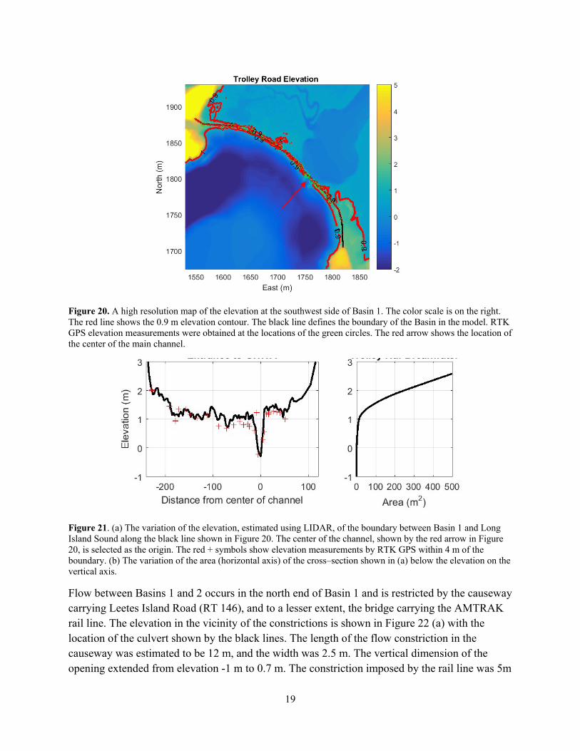
The main connection between GHWA and Long Island Sound is at the southwest boundary of Basin 1 where Trolley Road runs northwest and ends at the main channel into the GHWA marsh. The other side of the entrance has a low rock breakwater. It is likely that that this structure does not entirely block the exchange of water. The LIDAR derived elevation of this area is shown in Figure 20. The color code is on the right. The red line shows the 0.9 m contour and the thick black line shows the position of the boundary of Basin 1. We also conducted an RTKGPS survey of the elevation along this section and the green circles show the locations of measurements near the highest locations on the road. Figure 21 shows the variation of the elevation along the black line in Figure 20 together with the GPS measurements which are represented by the red + symbols. Most of the values cluster between 1 to 1.2 m, except in the narrow (approximately 20 m) channel which has a minimum elevation (maximum depth) at -0.3 m. Figure 21 (b) shows how the cross-sectional area of the flow across the boundary varies with water level. It is extremely small until the water exceeds 1 m and then increases in an approximately linear fashion.

19

 

Figure 20. A high resolution map of the elevation at the southwest side of Basin 1. The color scale is on the right. The red line shows the 0.9 m elevation contour. The black line defines the boundary of the Basin in the model. RTK GPS elevation measurements were obtained at the locations of the green circles. The red arrow shows the location of the center of the main channel.

 

Figure 21. (a) The variation of the elevation, estimated using LIDAR, of the boundary between Basin 1 and Long Island Sound along the black line shown in Figure 20. The center of the channel, shown by the red arrow in Figure 20, is selected as the origin. The red + symbols show elevation measurements by RTK GPS within 4 m of the boundary. (b) The variation of the area (horizontal axis) of the cross–section shown in (a) below the elevation on the vertical axis.

Flow between Basins 1 and 2 occurs in the north end of Basin 1 and is restricted by the causeway carrying Leetes Island Road (RT 146), and to a lesser extent, the bridge carrying the AMTRAK rail line. The elevation in the vicinity of the constrictions is shown in Figure 22 (a) with the location of the culvert shown by the black lines. The length of the flow constriction in the causeway was estimated to be 12 m, and the width was 2.5 m. The vertical dimension of the opening extended from elevation -1 m to 0.7 m. The constriction imposed by the rail line was 5m

20

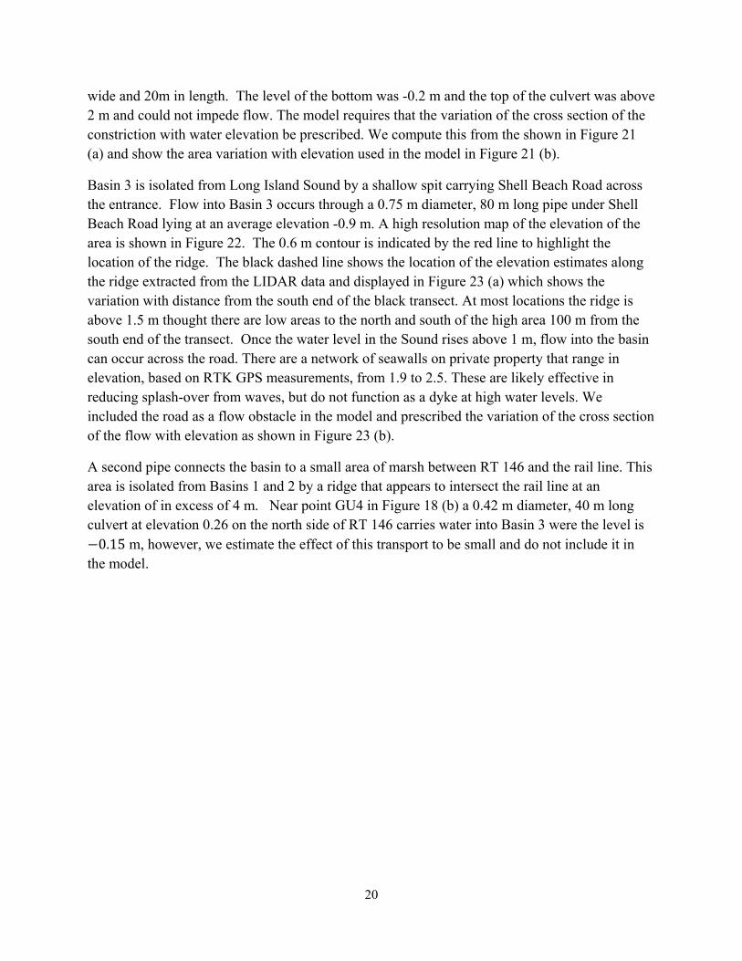
wide and 20m in length. The level of the bottom was -0.2 m and the top of the culvert was above 2 m and could not impede flow. The model requires that the variation of the cross section of the constriction with water elevation be prescribed. We compute this from the shown in Figure 21 (a) and show the area variation with elevation used in the model in Figure 21 (b).

Basin 3 is isolated from Long Island Sound by a shallow spit carrying Shell Beach Road across the entrance. Flow into Basin 3 occurs through a 0.75 m diameter, 80 m long pipe under Shell Beach Road lying at an average elevation -0.9 m. A high resolution map of the elevation of the area is shown in Figure 22. The 0.6 m contour is indicated by the red line to highlight the location of the ridge. The black dashed line shows the location of the elevation estimates along the ridge extracted from the LIDAR data and displayed in Figure 23 (a) which shows the variation with distance from the south end of the black transect. At most locations the ridge is above 1.5 m thought there are low areas to the north and south of the high area 100 m from the south end of the transect. Once the water level in the Sound rises above 1 m, flow into the basin can occur across the road. There are a network of seawalls on private property that range in elevation, based on RTK GPS measurements, from 1.9 to 2.5. These are likely effective in reducing splash-over from waves, but do not function as a dyke at high water levels. We included the road as a flow obstacle in the model and prescribed the variation of the cross section of the flow with elevation as shown in Figure 23 (b).

A second pipe connects the basin to a small area of marsh between RT 146 and the rail line. This area is isolated from Basins 1 and 2 by a ridge that appears to intersect the rail line at an elevation of in excess of 4 m. Near point GU4 in Figure 18 (b) a 0.42 m diameter, 40 m long culvert at elevation 0.26 on the north side of RT 146 carries water into Basin 3 were the level is 0.15 m, however, we estimate the effect of this transport to be small and do not include it in

the model.

21

 

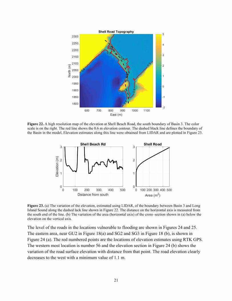
Figure 22. A high resolution map of the elevation at Shell Beach Road, the south boundary of Basin 3. The color scale is on the right. The red line shows the 0.6 m elevation contour. The dashed black line defines the boundary of the Basin in the model, Elevation estimates along this line were obtained from LIDAR and are plotted in Figure 23.

 

Figure 23. (a) The variation of the elevation, estimated using LIDAR, of the boundary between Basin 3 and Long Island Sound along the dashed lack line shown in Figure 22. The distance on the horizontal axis is measured from the south end of the line. (b) The variation of the area (horizontal axis) of the cross–section shown in (a) below the elevation on the vertical axis.

The level of the roads in the locations vulnerable to flooding are shown in Figures 24 and 25. The eastern area, near GU2 in Figure 18(a) and SG2 and SG3 in Figure 18 (b), is shown in Figure 24 (a). The red numbered points are the locations of elevation estimates using RTK GPS. The western most location is number 56 and the elevation section in Figure 24 (b) shows the variation of the road surface elevation with distance from that point. The road elevation clearly decreases to the west with a minimum value of 1.1 m.

22

 

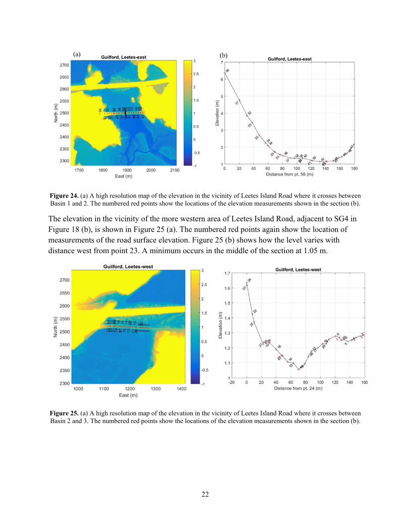
Figure 24. (a) A high resolution map of the elevation in the vicinity of Leetes Island Road where it crosses between Basin 1 and 2. The numbered red points show the locations of the elevation measurements shown in the section (b).

The elevation in the vicinity of the more western area of Leetes Island Road, adjacent to SG4 in Figure 18 (b), is shown in Figure 25 (a). The numbered red points again show the location of measurements of the road surface elevation. Figure 25 (b) shows how the level varies with distance west from point 23. A minimum occurs in the middle of the section at 1.05 m.

 

Figure 25. (a) A high resolution map of the elevation in the vicinity of Leetes Island Road where it crosses between Basin 2 and 3. The numbered red points show the locations of the elevation measurements shown in the section (b).

23

3.2 Observations

Measurements GU2 were successfully obtained from October 13th, 2016 to November 24th, 2016. Unfortunately, the data recovery from the instruments at the surrounding locations was not successful. Figure 26 (a) shows the time series of water level at GU2, which was located at the northern end of Basin 1, as the red line together with the water level at New Haven as the black line. These records are separated in the subtidal and tidal frequency components using a 5th order Butterworth filter with a 48 hour cut-off period and the resulting series are shown in Figures 26 (b) and (c). Note that the scale in (b) is different from the others.

To acquire sufficient data to tune and evaluate the model of water levels adequately, we redeployed instruments at the sites shown in Figure 18 (b) between April and June 2017. The measurements are shown in Figure 27 (a). The amplitude and variability of the New Haven water level is clearly shown by the black line. Though it is almost impossible to see in this display, the record from station SG1 (at the entrance of the marsh system) is shown in red. The much smaller amplitudes of the variation at SG2 (blue) and SG3 (green) are also clear and illustrates the substantial impact of the flow constrictions at the entrance to the marsh and the road bridge. The tidal frequency variation in Basin 3 at SG4 (cyan) is almost imperceptible. Figure 27 (b) shows the same records after a 5th order Butterworth filter with a 48 hour cut-off period has been applied to suppress the oscillations at the dominant semi-diurnal frequencies. This presentation reveals that the water levels vary with an amplitude of approximately 0.2 m in a manner that is coherent across the study area. It is also evident that though the flow constrictions have a major effect on the exchange at tidal frequencies, the low frequency fluctuations are much less damped. Figure 27 (c) shows original record with the low pass filtered record subtracted to reveal the tidal oscillations. The observation period was chosen to span two spring tides and the intervening neap and this is clear in the figure.

24

 

Figure 26. (a) The Red line shows the observations of sea level in GHWA at site GU2 and the black line shows the tide gage observations at New Haven CT. (b) The red and black lines show the aperiodic variations in the water level at the GU2 and New Haven sites not associated with semidiurnal tide and (c) show the tidal variations.

 

25

 

Figure 27. (a) The red, blue, green, and cyan lines shows the observations of sea level in GHWA during second observation campaign at sites SG1, SG2, SG3, and SG4, between April and June, 2017. The black line shows the tide gage observations at New Haven CT. (b) The lines show the aperiodic variations in the water level due to meteorological events at the same stations, and with the same color codes, as (a), and (c) show the tidal variations.

3.3 Results

Since Basin 3 is effectively isolated from the other we model it by a single equation forced only by flow across the Shell Beach Road. It is discussed separately in Section 3.3.2.

3.3.1 Basins 1 and 2

A model of the fluctuations in water level in Basins 1 and 2, based on that of O’Donnell et al. (2016), was developed using the observations at SG1 as the forcing and the observations at SG2 and SG3 to refine the coefficients describing the exchange between the Basins. The sea level at Long Island Sound in shown by the blue line in Figure 28 and the solution for the water level in Basin 1 using the optimal parameter set is shown by the red line. The green line shows the

26

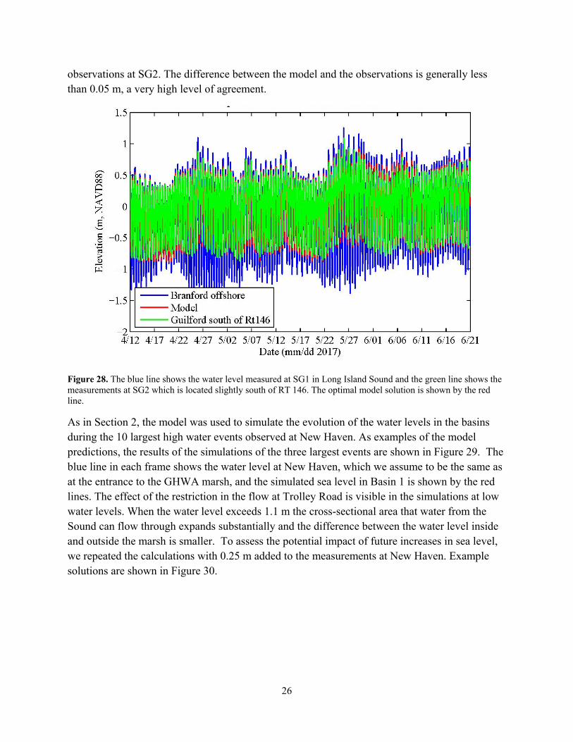
observations at SG2. The difference between the model and the observations is generally less than 0.05 m, a very high level of agreement.

 

Figure 28. The blue line shows the water level measured at SG1 in Long Island Sound and the green line shows the measurements at SG2 which is located slightly south of RT 146. The optimal model solution is shown by the red line.

As in Section 2, the model was used to simulate the evolution of the water levels in the basins during the 10 largest high water events observed at New Haven. As examples of the model predictions, the results of the simulations of the three largest events are shown in Figure 29. The blue line in each frame shows the water level at New Haven, which we assume to be the same as at the entrance to the GHWA marsh, and the simulated sea level in Basin 1 is shown by the red lines. The effect of the restriction in the flow at Trolley Road is visible in the simulations at low water levels. When the water level exceeds 1.1 m the cross-sectional area that water from the Sound can flow through expands substantially and the difference between the water level inside and outside the marsh is smaller. To assess the potential impact of future increases in sea level, we repeated the calculations with 0.25 m added to the measurements at New Haven. Example solutions are shown in Figure 30.

27

 

Figure 29. The sea level at New Haven is shown by the blue line in each frame and the simulated sea level in Basin 1 is shown by the red lines. The dotted red lines show the level of Daniels Avenue and the dashed red line show the level (1.1 m) of Leetes Island Road (RT 146).

 

Figure 30. The sea level at New Haven plus 0.25 m is shown by the blue line in each frame and the simulated sea level in Basin 1 is shown by the red lines. The dotted red lines show the level of Daniels Avenue and the dashed red line show the level (1.1 m) of Leetes Island Road (RT 146).

28

We show in Figure 31 the maximum values of the water level at New Haven during the largest 10 events observed between 1991 and 2016 by the blue squares connected by the blue line. The largest (super storm Sandy) is plotted at 1 and the others in rank order decreasing to the right. The high water level during all 10 storms exceeds 1.5 m at New Haven. The simulated water level in Basin 1, and at the eastern area of Leetes Island Road (see Figure 24) is shown by the red circles connected by the red line. With the exception of the two largest storms, the maximum water levels in Basin 1 were just above 1.1 m, the lowest level of the eastern section of Leetes Island Road in the study area. The peak levels in the marsh are approximately 0.5 m lower as a consequence of the constriction the flow into the marsh experiences and the limited time that the storm water level is high during most storms. The distance between the solid blue and red lines is a measure of the flood protection value provided by the marsh volume and the flow constriction at Trolley Road. However, during the two largest events (Hurricane Irene and super storm Sandy) the water level in the Sound was substantially higher than in the other storms, and higher for longer, and those factors allowed more water to get into the marsh system causing much more substantial flooding on the road and the land surrounding the marsh. The protective value of the marsh is significant for most storms but diminishes during the largest storms.

 

Figure 31. A summary of the simulations of the 10 largest water level events in New Haven. The blue line and squares show the maximum water levels observed at New Haven and the red line and circle symbols show the predicted level in marsh Basin 1. The dotted black line at 1.1 m shows the level of Leetes Island Road (RT 146). The dashed red line and the dashed blue line show the marsh and New Haven levels if mean sea level was 0.25 higher.

29

The effect of future sea level rise on the area was investigated by adding 0.25 m to the New Haven water level and repeating the analysis. The blue dashed line in Figure 31 shows the augmented sea level at New Haven and the red dashed line shows the peak values in the simulated level in the marsh. The difference between the dashed lines is similar to the existing condition showing that the marsh and entrance will continue to provide flood protection value, however, Leetes Island Road will be flooded more often and to a higher level. A plausible option to significantly reduce the flooding frequency would be to increase the level of the level of Trolley Road and the berm to the west of the entrance to the marsh.

3.3.2 Basins 3

The model of the water levels in Basin 3 was developed to assess the flooding risk at the western end of Leetes Island Road (RT 146) as shown in the map in Figure 25. In the low area of the road the elevation was measured by RTKGPS as 1.1 m. The model coefficients were selected to achieve an optimal agreement between the measurement at SG4 and the model predictions. In Figure 32 we show the water level measured in Long Island Sound at SG1 by the black line and the level at SG4 by the red line. Note that we truncated the record at May 25 since the variance in the SG4 series appeared anomalously low after that, perhaps as a result of biofouling. The effect of the flow restriction in damping the water level fluctuations in this area is obvious. Even though the amplitude of the water level fluctuations in the sound reaches 1.4 m the level in the marsh is only 10% as large.

 

Figure 32. A comparison of the model predictions (green line) and the measurements at SG4 (red line) between April and May, 2017 when the water level measured at SG1 in Long Island Sound fluctuated as shown by the black line.

30

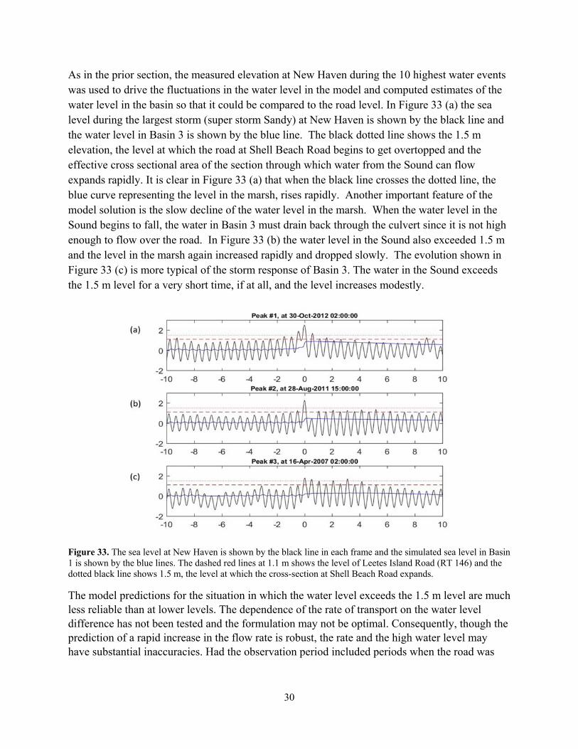
As in the prior section, the measured elevation at New Haven during the 10 highest water events was used to drive the fluctuations in the water level in the model and computed estimates of the water level in the basin so that it could be compared to the road level. In Figure 33 (a) the sea level during the largest storm (super storm Sandy) at New Haven is shown by the black line and the water level in Basin 3 is shown by the blue line. The black dotted line shows the 1.5 m elevation, the level at which the road at Shell Beach Road begins to get overtopped and the effective cross sectional area of the section through which water from the Sound can flow expands rapidly. It is clear in Figure 33 (a) that when the black line crosses the dotted line, the blue curve representing the level in the marsh, rises rapidly. Another important feature of the model solution is the slow decline of the water level in the marsh. When the water level in the Sound begins to fall, the water in Basin 3 must drain back through the culvert since it is not high enough to flow over the road. In Figure 33 (b) the water level in the Sound also exceeded 1.5 m and the level in the marsh again increased rapidly and dropped slowly. The evolution shown in Figure 33 (c) is more typical of the storm response of Basin 3. The water in the Sound exceeds the 1.5 m level for a very short time, if at all, and the level increases modestly.

 

Figure 33. The sea level at New Haven is shown by the black line in each frame and the simulated sea level in Basin 1 is shown by the blue lines. The dashed red lines at 1.1 m shows the level of Leetes Island Road (RT 146) and the dotted black line shows 1.5 m, the level at which the cross-section at Shell Beach Road expands.

The model predictions for the situation in which the water level exceeds the 1.5 m level are much less reliable than at lower levels. The dependence of the rate of transport on the water level difference has not been tested and the formulation may not be optimal. Consequently, though the prediction of a rapid increase in the flow rate is robust, the rate and the high water level may have substantial inaccuracies. Had the observation period included periods when the road was

31

over-topped, the empirical constants and the flow rate parameterizations could have been improved and more accurate predictions developed.

The characteristics of the impact of an increase in sea level were examined by repeating the simulations of the storm water levels. Figure 34 shows the same results as in Figure 33 but with 0.25 m added to the water level at New Haven. This brings the high tide level much closer to the level of Shell Beach Road and so smaller storms can lead to over-topping and higher levels in marsh Basin 3. However, the levels predicted when overtopping occurs is not as accurate.

The results of the simulations of the ten highest water events at New Haven are shown in Figure 35. The red squares joined by the red line show the high water levels in descending rank order and the highest levels predicted for Basin 3 of the marsh are shown by the blue + symbols joined by the blue line. Though all the storms led to high water above the 1.5 m level of Shell Beach Road, the flow over the road did not last long enough for the volume to raise the level in the marsh to a level close to RT 146, except for the two most severe storm, super storm Sandy and Hurricane Irene. The value of Shell Beach Road and the storage volume of the marsh as flood protection for Leetes Island Road (RT 146) for most storms is substantial as measured by the difference between the blue and solid red lines in Figure 35. Even during super storm Sandy the model only predicts a maximum water level of 0.9 m, though this is uncertain. The vulnerability to road flooding in this area is low, though exceptional storms would likely fill the marsh basin and led to flooding

 

Figure 34. The sea level at New Haven with 0.25 m added, to represent a future increase, is shown by the black line in each frame and the simulated sea level in Basin 1 is shown by the blue lines. The dashed red lines at 1.1 m shows the level of Leetes Island Road (RT 146) and the dotted black line shows 1.5 m, the level at which the cross-section at Shell Beach Road expands.

32

 

Figure 35. A summary of the simulations of the 10 largest water level events in New Haven. The red line and squares show the maximum water levels observed at New Haven and the blue line and + symbols show the predicted level in marsh Basin 3. The black dashed line shows the level of Leetes Island Road (RT 146) and the dotted line shows the level of Shell Beach Road. The red dashed line the New Haven water level peaks with 0.25 m added and the magenta line and circles show the peaks in the model predicted series for the level in the marsh.

3.4 Summary

We deployed instruments to measure water level fluctuations in the marsh complex of the Great Harbor Wildlife Area so that we could develop simulations of the water level fluctuations during severe storms. The analysis of the geometry and the water level elevation measurements showed that the two basins to the east were hydrodynamically linked, but the western basin was only forced by water levels in the Sound through a separate connection. Two models were developed and shown to perform adequately. Simulations showed that eastern section of Leetes Island Road (RT 146) is protected from flooding by the flow constriction at Trolley Road, and the volume storage capacity of the marsh though during the worst storms of the year water likely reaches the road surface. During the two most severe storms the flood protection value is eliminated. A small increase in sea level will lead of much more frequent and severe flooding in this area. Raising the level of Trolley Road is an adaptation option worthy of consideration.

In the western area of the marsh complex, the flow constriction at Shell Beach Road limits the vulnerability of the Leetes Island Road (RT 146) section to flooding to only the most severe storms. Since the high water level predicted at the road is sensitive to the volume flux over the

33

road, and this could not be accurately parameterized in the model, more observations are required in order to evaluate strategies for further reduce the risk of flooding during events like Hurricane Irene and super storm Sandy.

34  

4. Study Area 3 –Indian Neck Avenue and RT 146

4.1 The Geometry

Figure 2 shows Study Area 3 and the area of the Branford River where Indian Neck Avenue and RT 146 cross the Branford River and then pass under the AMTRAK line to the north. Figure 35 (a) shows the topography and bathymetry in the study region relative to NAVD88 using the USGS (2017) digital elevation model constructed from LIDAR. This data was obtained from https://coast.noaa.gov/dataviewer/. The main river channel allows water from the Sound to flow eastward and then northward into the center of the town. The white + symbols show the locations of instruments we deployed in 2016.

 

Figure 35. (a) A map of the elevation and bathymetry of the Branford, CT, created using the USGS (2017) which was based the LIDAR measurements. The location of sensors to record water level are shown by the white crosses. (b) shows a higher resolution view of Study Area 3. The bridges across the Branford River, and the Approach roads are shown in black.

A higher resolution map of the study area is shown in Figure 35 (b) with the locations of the Indian Neck Avenue and RT 146 where they cross the Branford River indicated in black. The AMTRAK line is clearly visible in the map as the linear feature at the northern shore of the Branford River. Both Indian Neck Avenue and RT 146 cross underneath the rail line on the north side of the river at the northern end of the black lines.

Figure 36 (a) shows the north-south variation of the elevation of the RT 146 road surface along the section indicated in black in Figure 35 (b). The black line shows the highest and lowest values in the digital elevation map within 2 m of the line in Figure 35 (b). The red squares show levels measured by an RTK GPS system and the red line show the approximate level of the bridge surface. The low values (1.6 m) on the right (north) of the graph show where RT 146 goes under the rail line. The large variation is due to the proximity of the rail line bed. The low values

35  

(0.1 m) in the north of the section of Indian Neck Ave shown in Figure 36 (b) are also where the road goes under the Rail line.

Figure 36. The north-south variation of the elevation of (a) RT 146, and (b) Indian Neck Avenue, along the sections shown in Figure 35 (b). The red lines show the approximate level of the road on the bridge. The black dashed lines shows the levels at which road flooding occurs.

Since the locations of the low road levels is not immediately adjacent to the Branford River, the intervening topography determines the level at which flow into the low areas can occur. Figure 37 (a) shows a high resolution view of the topography near the low area of Indian Neck Road and the Branford River. The color scale is on the right of the Figure and spans the interval -2 to 5 m NAVD88 to emphasize the variation at low elevations. The thick black line is the 2 m contour and the thin black line is the 1.75 m level. The section of Indian Neck Avenue shown by the black line in Figure 35 (a) and 36 (b) is labeled in the bottom left side of Figure 37 (a) where it enters the lowest part of the roadway. The contours show that when the water level exceeds 1.75m there is a pathway for water to flow under the rail line to cause road flooding. This flow can then continue into the extensive low area to the north of the rail causeway. The 1.75 m elevation is shown on the road elevation section in Figure 36 (b) as the black dashed line. Figure 37 (b) show the detailed structure of the elevation in the area of the RT 146 rail underpass. Again the thick black line shows the 2 m elevation contour, but the elevation at this location depicted most clearly using the 1.7 m (thin black line) and the 1.5 m (thin dashed line) contours. It is clear

36  

that when the water level exceeds 1.6 m at the shore it can flow into the underpass and flood RT 146. This level is shown in Figure 36 (a).

Figure 37. High resolution maps of the elevation in (a) the Indian Neck Avenue Area. The color scale (m) is shown on the right. The thick black line is the 2m elevation contour and the thin line is the 1.75 m contour. The elevation in the RT 146 rail underpass area is shown in (b). The 2 m contour is shown by the thick black line and the thin line shows the 1.5 m contour.

4.2 Observations.

To quantitatively relate the variations in water level in the Sound and those in the Study Area, we deployed water level sensors at the locations shown by the white + symbol in Figure 35 (a). The details of the equipment and the deployment times and dates are provided in Appendix 2. The sensor at BR4 characterized the level just outside the mouth of the Branford River and the sensor at BR3 recorded the level in the Study Area. The NOAA tide gage at New Haven was also used to provide longer term observations. The NOAA tide station at Branford (8465233) (see NOAA, 2017a) reports that the mean sea level is at -0.086 m relative to NAVD88. The currently active gage at New Haven (8465705) has not been referenced to NAVD, however, an earlier one (8465748, NOAA, 2017b) reported mean sea level as -0.076 m NAVD. Since determining the level of the sensors relative to NAVD88 in deeper water was problematic, we set the mean of the observations at BR1, BR2 and BR3 equal to NAVD88 level -0.086 m. We then assume that the mean of the record obtained from the New Haven gage is equal to the same value. These assumptions lead to errors. There is unlikely to be more than a few centimeters difference in the long term mean levels at Branford and New Haven, however, there are seasonal variations in the

37  

mean water level that are uniform across Long Island Sound. At New Haven the mean water level between October and January is not significantly different from the annual mean and has a standard deviation of 0.07 m. The variation in the annual mean over the last three decades has a similar magnitude. We estimate that the error in our level estimates relative to NAVD88 is, therefore, 0.1m.

Figure 38 (a) shows the time series of water levels measured at BR1, BR3, BR4 and New Haven in the October –December 2016 observation period relative to NAVD88. The variability in values spans 1. 4 m and is dominated by the semidiurnal tides. The differences between the four series are relatively small and difficult to detect. In Figure 38 (b) we show the same series after the tidal periods fluctuations have been suppressed out by a 5th order Butterworth filter with a cut-off period of 28 hours (see Emery and Thomson, 2001). The difference between the original series and the filtered series are shown in Figure 38 (c) which show the tidal oscillations more clearly. These series display the response of the water in the Sound to the effects of the local wind and variations of water level on the continental shelf. The magnitude of the fluctuations range between -.5 and .4 m. The only site that shows any substantial difference from the others is BR4 (black line). This is likely due to the coastal geometry and the influence of high frequency waves. A seven day segment of the same data are shown in Figure 39 to illustrate more clearly how little difference there is between the observations at New Haven and in the study area (BR1 and BR3).

 

Figure 38. (a) The time series of the water elevations measured at BR1, BR2, BR3 and New Haven with the low-pass filtered records shown in (b). The high-pass records are in (c).

A comparison of the level of the maximum values that occur in each 12.4 hour tidal period during the observation interval in Study Area 3 is shown in Figure 40. The correlation between

38  

the values is obviously very high and the slope of the best-fit line defined by least-squares regression is not significantly different from unity. The BR3 observations lag those at New Haven by less than an hour. The root mean square difference between the values is 0.1 m. We conclude that the observations at New Haven can be used to estimate the level in the study area directly. 

 

Figure 39. These graphs show a 7 day section of the records in Figure 38. a) The time series of the water elevations measured at BR1, BR2, BR3 and New Haven with the low-pass filtered records shown in (b). The high-pass records are in (c).

 

Figure 40. The observed maximum water levels at BR3 (vertical axis) and at New Haven (horizontal axis) during each tidal period of the observation period in Study Area 3.

39  

4.3 Analysis

The observations shown in Figure 37 demonstrates that there is no need for a model to describe the differences between the water levels at New Haven and the study area. The propagation of the tide up the channel of the Branford River from the Sound appears to be such that the dissipation of energy by bottom friction is compensated for by the convergence of the channel cross-section so that the amplitude of the major constituents are not noticeably diminished. The hourly water level variations due to tides alone predicted by NOAA at New Haven since 1999 are shown in Figure 41 (a). The maximum values are just below 1.5 m and so at current mean sea level water levels exceed the flood thresholds in the study area only during storm surges. The black curve in Figure 41 (b) shows how many days per year (averaged over 17 years) the maximum water level exceeds the values shown on the vertical axis. The red line shows the same thing if the mean sea level was raised 25 cm. There is a substantial effect at the RT 146 underpass which will be flooded on approximately 14 days in an average year.

 

Figure 41. (a) Tidal water level fluctuations (relative to the approximate NAVD88 datum) at New Haven and Branford predicted by NOAA. (b) The black line shows the number of days per year (horizontal axis) in which the maximum water level exceeds the level shown in the vertical axis. The dashed line shows the 1.75 m flooding threshold at Indian Neck Avenue, and the dotted line shows the 1.6 m threshold at the RT 146 underpass. The red line shows the effect of a 0.25 m sea level increase.

Figure 14 shows the observations at New Haven since 1999. These data include both the effects of tide and wind induced fluctuations. Table 1 lists magnitude and date of the top 10 water levels observed. These levels are also expected to have occurred in the study area. Figure 42 shows the

40  

elevation of the 20 largest sea level peaks in the record form New Haven by the red squares together with the elevation of the critical levels at the Indian Neck Avenue and RT 146 railway underpasses. It is evident that the many storms currently lead to the threshold being exceeded at RT 146 and that the Indian Neck Avenue threshold is exceed 7 time in 17 years. Note that the maximum elevations in storms 3 to 20 range from 1.7 to 1.9 m so a small increase in mean sea level will lead to a very large increase in the risk of flooding. The blue line illustrates the effect of a 0.25 m increase in mean sea level. This would cause both underpasses to be flooded

 

Figure 42. The red line and square symbols show the maximum elevation of the largest peaks in the sea level record at New Haven since 1999. These levels are compared to the elevation of the threshold for road flooding at Indian Neck Road (short dashes) and RT 146 (longer dashes). The blue line show the maximum level plus 0.25 m to illustrate the effect of a future increase in sea level.

The best assessment of the vulnerability of a site to coastal flooding must take into account the joint effects of tides and storm surges. NOAA (Zervas, 2013) has computed the probability of water elevations exceeding prescribed values at most tide stations, including Bridgeport and New London, but has not analyzed the record at New Haven. The U.S. Army Corp of Engineers (USACE, 2015) has published the results of a model study of water level variability and provided on-line access to the numerical results at a wide variety of locations in the northwest Atlantic and Long Island Sound. These two studies use very different approaches to estimate the probability of the water level at a site exceeding a threshold in any year and yield significantly different results. The thick cyan line in Figure 43 shows the NOAA (Zervas, 2013) estimate of the probability of the water level shown on the vertical axis being exceeded in a year at Bridgeport, CT, the closest available station where the analysis has been published. Note that the inverses of the probability (the return interval in years) is plotted on the horizontal axis. The USACE (2015) analyses at points near Bridgeport and New Haven are shown by the thick solid and dashed lines respectively. These differ substantially for return interval greater than 5. This

41  

reflects the difference in the approaches as well as the uncertainty arising from the relatively short data record. The red squares show the largest peaks, separated by more than 24 hours, in the available water level record at the NOAA tide gage in New Haven after the variations in the annual mean and long term trend has been eliminated. The red line is the generalized Pareto function that is the best-fit to the data points. It is clear that the NOAA and USACE estimates are biased high relative to the observations at New Haven, especially at the short return intervals, and are therefore not very useful in the evaluation of the flooding frequency changes. These sources may be better used for assessing the magnitude of very unusual events.

The green dashed horizontal lines in Figure 43 shows the level of flooding thresholds for the Indian Neck Avenue and the RT 146 railway underpasses. Comparison of these level to the red squares and red line shows that RT 146 is at the level that should be expected to flood every year, whereas the Indian Neck area would have approximately a 25% chance of flooding each year, or a 4 year return interval. It is important to reiterate hear that the mean water level in Long Island Sound varies from year to year by 0.05-0.1 and that the uncertainty in the leveling of gages leads to a similar error. The impact of these imperfections in knowledge is that the risk of flooding at RT 146 is in the range 200-50% each year, and at Indian Neck Avenue is 20%-30% each year.

 

Figure 43. The thick cyan line shows the NOAA (Zervas, 2013) analysis of the probability (yr-1) of the level shown in the vertical axis being exceeded in a year at Bridgeport (8467150). Note that the inverse of the probability, or return interval (yr), is plotted on the horizontal axis. The thick black solid and dashed lines show the same statistics at a location near Bridgeport and New Haven, respectively, estimated by the UASCE (2015). The red squares and the red line show the larges values of total water level measured at New Haven since 1999 and the generalized Pareto function that is the best fit to the points.

42  

If the means sea level was to increase by 0.25 then the empirical distribution shown in red in Figure 43 would be transformed to the one shown by the thin blue line. This is well above both the flood thresholds, indicating that these locations would be likely to flood many times each year. The geometry of the coast in the study area may make flood barriers practical, however, to reduce the flood risk to 10% per year (a 10 year return interval) at current sea levels would require the structure to be at least 2 m above NAVD88. If the 1% threshold was the design goal then the NOAA analyses (cyan line in Figure 43) would suggest 2.56 m would be necessary.

4.4 Summary

We have examined water level fluctuations in the Branford River and show that they are almost identical to those observed at the tide gage in New Haven. We used LIDAR and RTK GPS surveys to establish the elevation of areas that are prone to flooding by the Branford River. Currently, ordinary tidal variations do not cause flooding of the Indian Neck underpass or the RT 146 underpass, however, a 0.25 m rise in the mean sea level will lead to the RT 146 underpass being flooded on approximately 14 days per year. When the effects of meteorological variations are also taken into account, the underpass at RT 146 is at the level that should be expected to flood every year, whereas the Indian Neck area has a 25% chance of flooding each year, or a 4 year return interval. These areas are, therefore, extremely vulnerable to sea level rise and a 0.25 m increase would cause both to be flooded more than ten times a year.

` 

43  

5. Study Area 4, Linden and Sybil (RT 146) Avenues

5.1 The Geometry

A bridge and tide gate carry RT 146 across the Sybil Creek in Branford. Figure 44 shows the topography and bathymetry in the area of the bridge and the location of 4 moored instruments that were deployed to observe water level fluctuations. Flooding have been reported on both Sybil and Linden Avenue to the east of the bridge. The magenta square in Figure 44 includes BR1 and BR2 and surrounds the area prone to flooding. A high resolution map of the area is shown in Figure 45 where the elevation range displayed is restricted to -0.5 m to 2m to reveal the subtle variations in topography around the level of the top of the bridge. The red dots in Figure 45 indicate the locations of measurements of elevation by RTK GPS (see Appendix 2) on the road surface of the tide gate-bridge structure.

 

Figure 44. The topography and bathymetry of Branford, CT. The color codes are shown on the right. The square defined by the dashed magenta line surrounds the junction of Sybil and Linden Avenue and defines the area shown in higher resolution in Figure 45. The white + symbols show the location of moored instruments. The area surrounded by the cyan square is discussed in the next section.

The black line in Figure 46 displays the elevation along a north-south line through the red points in Figure 45 using both LIDAR estimates and the direct RTKGPS measurements. The data show that the top of the tide gate is at 1.9 m NAVD88 and the level of the bottom of the channel near the structure is 0.7 m. These measurements are clearly consistent with each other. It is worthy of note that the bridge is scheduled for replacement and the design (90% final) shows it to be at the level 1.96 m (NAVD88).

` 

44  

 

Figure 45. A high resolution map of the elevation in the area of Linden and Sybil Avenue. The color range is set to vary from -0.5 to 2.0 m NAVD to highlight the variation in the elevation in this range. The red dots show the locations where elevation on the road surface at the tide-gate and bridge structure at Linden Avenue was measured with an RTK GPS system.

 

 

Figure 46. The black line shows elevation estimates along Sybil Avenue from the LIDAR shown in Figure 45, and the red + symbols and line shows measurements by RTK GPS at the locations shown by the red points in Figure 45.

` 

45  

5.2 The Observations

The observations from sites BR1, BR2 and the sea level measurements from the NOAA tide gage at New Haven are shown in Figure 47. The mean over the common period of observation of the New Haven and BR1 series was set to -0.08 NAVD, which is the mean sea level reported by NOAA when they maintained a station in Branford (8465233). This was necessary because the NOAA gage in New Haven is not referenced to NAVD directly, and because measuring the water level at the sensors during the deployment was difficult and the consequent uncertainties were too large for the datum to be useful. In Figure 47 (a) we show the evolution of the total water level for all three series. The magnitude of the tidal oscillations, the spring-neap cycle, and the irregular meteorologically forced motions are all evident. but since the differences between the records are so small, the different lines are difficult to distinguish. In Figure 47 (b) we show the same series after the semidiurnal tidal oscillations have been removed by a 5th order Butterworth filter with a 48 hour cut-off period. The New Haven (cyan) and the BR1 (red) series are again almost coincident demonstrating that the low frequency variations propagate from the Sound into Branford harbor with little variation. The dark blue line shows the BR2 record. This record has been adjusted to the NAVD88 datum (approximately) by minimizing the difference between the peaks in the low-pass filtered series at BR1 and BR2. This allows the tidal frequency variations, see Figure 47 (c), to be influenced by the bathymetry, but not the low frequencies.

 

Figure 47. (a) Time evolution of the water level observed at BR1 (red), BR2 (blue) and New Haven (cyan) in the fall of 2016. (b) The low pass filtered series and (s) show the high frequency signal.

To compare the observations more clearly we show in Figure 48 a seven day segment of the same data as in Figure 47. The only noticeable difference in the raw series shown in Figure 48 (a) is that the BR2 series (blue lines) doesn’t fall below -0.6 m which is the elevation of the bottom a at the station location. The low frequency variation shown in Figure 48 (b) also shows

` 

46  

that the BR2 series (blue) varies from the others, it usually higher, largely as a consequence of the higher minimum value that it can reach.

The maxima in the total water level records from BR2 and New Haven during the observation period are compared in Figure 49. The root mean square difference in the maxima is 0.05 m and the correlation coefficient is 0.98. This demonstrates that there is little difference between the two levels and there is, therefore, no need for a model of the flow in the lower Branford River to link the two levels.  

 

Figure 48. The same data as in Figure 4 but for a 7 day interval in November 2016.

 

Figure 49. The correlation between the magnitude of the peaks observed in the New Haven (horizontal axis) and BR2 (vertical axis) series shown in Figure 4 (a).

` 

47  

5.3 Analysis

The measurements described in the preceding section demonstrate the water level at BR2 and the junction of Linden and Sybil Avenues can be accurately represented by the NOAA water level at New Haven. The analysis of the LIDAR and RTK GPS elevation measurements indicate that the roads are subject to flooding by seawater when the water level exceeds 1.9 m NAVD88. Figure 14 shows the record of sea level reported by NOAA at New Haven in the seventeen years since January, 1999, with the 20 highest levels (separated by at least 48 hours) highlighted by the red circles. These values are shown in descending rank order by the red squares in Figure 50. Note that these level assume that the mean sea level at New Haven (and BR1) is -0.08 m NAVD and this may introduce an error of approximately 0.1 m. The largest two values exceed 2 m and occurred during Hurricane Irene in August, 2011, and super-storm Sandy in October 2012. The rest of the peaks were due to the much more frequent extra-tropical storms. The dashed black line shows the level of the roadway at Linden and Sybil Avenues where it crosses Sybil Creek. This graphic suggests that the roadway was flooded during the hurricanes and perhaps the next two largest water level peaks. The levels reached by the peaks ranked 5 and higher lie below the road level in a narrow range between 1.7 and 1.9 m. That the level of the roadway was reached or exceed four times in seventeen years confirms that the area is at risk from coastal flooding. The red dashed line shows the levels that the water level peaks would have reached if mean sea level had been 0.25 m higher, a level that could plausibly occur by 2050. Comparison of the red and the black dashed lines demonstrates that all 20 storm could cause road flooding in the future.

 

Figure 50. The red squares show the levels of the 20 highest water levels observed at New Haven since January 1999. The dashed black line shows the level 1.9 m, which is the elevation of the road surface at the bridge across Sybil Creek. The dashed line is the levels that the water levels would have reached of the means sea level was 0.25 m higher.

` 

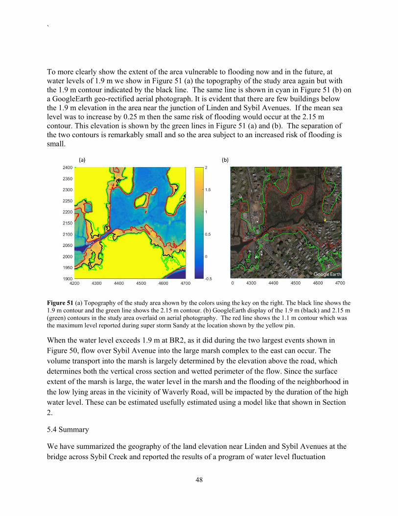
48  

To more clearly show the extent of the area vulnerable to flooding now and in the future, at water levels of 1.9 m we show in Figure 51 (a) the topography of the study area again but with the 1.9 m contour indicated by the black line. The same line is shown in cyan in Figure 51 (b) on a GoogleEarth geo-rectified aerial photograph. It is evident that there are few buildings below the 1.9 m elevation in the area near the junction of Linden and Sybil Avenues. If the mean sea level was to increase by 0.25 m then the same risk of flooding would occur at the 2.15 m contour. This elevation is shown by the green lines in Figure 51 (a) and (b). The separation of the two contours is remarkably small and so the area subject to an increased risk of flooding is small.

 

Figure 51 (a) Topography of the study area shown by the colors using the key on the right. The black line shows the 1.9 m contour and the green line shows the 2.15 m contour. (b) GoogleEarth display of the 1.9 m (black) and 2.15 m (green) contours in the study area overlaid on aerial photography. The red line shows the 1.1 m contour which was the maximum level reported during super storm Sandy at the location shown by the yellow pin.

When the water level exceeds 1.9 m at BR2, as it did during the two largest events shown in Figure 50, flow over Sybil Avenue into the large marsh complex to the east can occur. The volume transport into the marsh is largely determined by the elevation above the road, which determines both the vertical cross section and wetted perimeter of the flow. Since the surface extent of the marsh is large, the water level in the marsh and the flooding of the neighborhood in the low lying areas in the vicinity of Waverly Road, will be impacted by the duration of the high water level. These can be estimated usefully estimated using a model like that shown in Section 2.

5.4 Summary

We have summarized the geography of the land elevation near Linden and Sybil Avenues at the bridge across Sybil Creek and reported the results of a program of water level fluctuation

` 

49  

observations. The latter show that the water levels at the bridge are almost equal to those reported at the NOAA tide gage at New Haven. The longer data record available there allows us to characterize the longer term variability of the water levels and to describe the vulnerability of the area to flooding by water from Long Island Sound. We show that in the last 17 years only two major hurricanes raised the water level above the road and two other storms were very close to the 1.9 m road level. However, the next biggest 16 peaks all caused water levels above 1.7 m so that an increase in mean sea level of just 0.25 m would lead to the road being flooded much more frequently. Since the slope of the topography at the 1.9 m level is relatively large in most of the study area, the 1.9 and 2.15 m contours are very close together. Consequently, the area of the study that is subject to an increase flooding risk is small. In addition to the increased frequency of closures of the Sybil Avenue Bridge, the main increase in flooding vulnerability will occur in the low lying areas near Waverly Road, when flow across the Sybil Avenue Bridge into the marsh to the east will occur more often. This could be assessed quantitatively using a model like that in section 2 and the benefits compared to the costs. This issue will be addressed further in the next section.

` 

50  

6. Study Area 5, Limewood Avenue (RT 146) and Waverly Road, Branford

RT 146 in Branford has a short section, Limewood Avenue, that follows the shoreline of Long Island Sound before turning north where it changes name to Sybil Avenue. During super-storm Sandy, the waves that impacted the shoreline from Long Island Sound overtopped the road. The water on Limewood Avenue then flowed down Waverly Road into the marsh surrounding Sybil Creek. The water in the marsh largely is isolated form the Branford River, and Long Island Sound, by the tide-gate at the Sybil Avenue Bridge. Unfortunately there were no direct measurements of the wave characteristics during the storm or of the water levels in the marsh. However, the USGS post storm high water mark surveys did locate a station in the marsh, see (https://stn.wim.usgs.gov/STNPublicInfo/#/HWMPage?Site=19322&HWM=18220). This will be used as an assessment of the effectiveness of the model predictions.

6.1 The Geometry

Figure 52 shows the elevation and bathymetry of the region derived from the USGS (2017) digital elevation model. The dotted magenta line along the shore in Figure 52 show the location of RTK GPS elevation measurement along the Limewood Avenue and the solid white line shows the location of Waverly Road. The dashed line from Limewood Road to BR4 shows the location of the water depth section in Figure 53.

 

Figure 52. Topography of the Limewood Avenue –Waverly Road area. The color scale show the elevation in the range -2 to 5 m using the color scale on the right. The location of the water level and wave sensors at BR 4 is shown by the white + symbol. The magenta points lie on Limewood Avenue and the solid white line shows Waverly Road.

` 

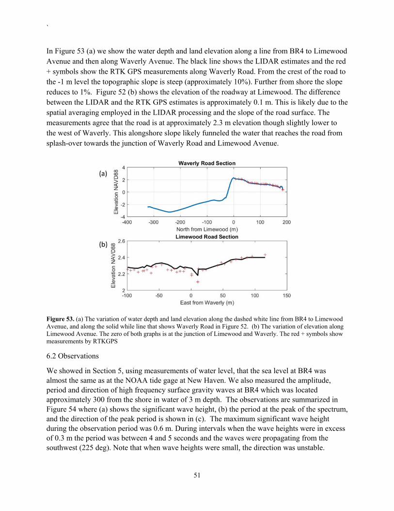
51  

In Figure 53 (a) we show the water depth and land elevation along a line from BR4 to Limewood Avenue and then along Waverly Avenue. The black line shows the LIDAR estimates and the red + symbols show the RTK GPS measurements along Waverly Road. From the crest of the road to the -1 m level the topographic slope is steep (approximately 10%). Further from shore the slope reduces to 1%. Figure 52 (b) shows the elevation of the roadway at Limewood. The difference between the LIDAR and the RTK GPS estimates is approximately 0.1 m. This is likely due to the spatial averaging employed in the LIDAR processing and the slope of the road surface. The measurements agree that the road is at approximately 2.3 m elevation though slightly lower to the west of Waverly. This alongshore slope likely funneled the water that reaches the road from splash-over towards the junction of Waverly Road and Limewood Avenue.

 

Figure 53. (a) The variation of water depth and land elevation along the dashed white line from BR4 to Limewood Avenue, and along the solid while line that shows Waverly Road in Figure 52. (b) The variation of elevation along Limewood Avenue. The zero of both graphs is at the junction of Limewood and Waverly. The red + symbols show measurements by RTKGPS

6.2 Observations

We showed in Section 5, using measurements of water level, that the sea level at BR4 was almost the same as at the NOAA tide gage at New Haven. We also measured the amplitude, period and direction of high frequency surface gravity waves at BR4 which was located approximately 300 from the shore in water of 3 m depth. The observations are summarized in Figure 54 where (a) shows the significant wave height, (b) the period at the peak of the spectrum, and the direction of the peak period is shown in (c). The maximum significant wave height during the observation period was 0.6 m. During intervals when the wave heights were in excess of 0.3 m the period was between 4 and 5 seconds and the waves were propagating from the southwest (225 deg). Note that when wave heights were small, the direction was unstable.

` 

52  

6.3 Model Results

Whether or not coastal flooding occurs on Limewood Avenue and Waverly Road is determined by the mean water level and the height and period of the storm driven waves. We have demonstrated in Section 5 that the water levels at Branford and New Haven are effectively the same. However, wave measurements close to shore in the area are limited and long records are only available at two buoys in the center of the Sound. To estimate the wave conditions during major storms we developed a mathematical model of the generation and propagation of waves in Long Island Sound and evaluated it with measurements at a variety of location. A summary of the project and results can be found at http://circa.uconn.edu/crest/wave-research/. The fundamental goal was to establish that the model adequately reproduced observations during major storm events at the buoy locations where data was available for 12 years. We then evaluated how well the model performed at several coastal sites where data had been acquired for several months. When the model was performing well in both tests we used it to generate statistics for waves that occurred at near shore location and published the results on the circa.uconn.edu web site. For this project we also tested the model at the BR4 site using the data shown in Figure 54.

A comparison of the model predictions to the observations at BR4 is provided in Figure 55. The black lines in Figure 55 (a) and (b) show the model significant wave height and the peak period, respectively, and the blue points show the observations. The root mean square error for the December 2016 simulation was 0.87 s for the dominant period, and 0.21 m for the significant wave height. The correlations were both very high as is evident in the figures. The significant wave height was biased low as we have found to be the case at other sites when the wind and waves were in the moderate range, however, at higher wind speeds the bias is less.

To summarize the wave amplitudes and periods that may be expected during severe storms, we simulated 20 storms with the high winds speeds. We used the wind speed data to rank the storms and constructed the return interval diagram shown in Figure 56 using the rank of the wind speed used in the model forcing for the return interval. Table 2 lists the maximum significant wave heights dominant periods in the simulations. The largest significant wave height occurred during Hurricane Carol in 1954 which produced a significant wave height of 3.84 m. Since the waves generated in Long Island Sound are generally fetch limited, the amplitude and period are correlated. Our simulation of super storm Sandy in 2012 was produced maximum significant wave heights near BR4 of 1.89 m with a dominant period of 7.4 s. Figure 56 suggests that the probability of exceeding this significant wave height value in any year is approximately 1/7.

` 

53  

 

Figure 54. Wave observations at BR4 from October 30, 2016 to January 8th, 2017. (a) shows the significant wave height (m), (b) the peak wave periods (s) and (c) shows the direction (degs.) the waves at the peak period were traveling from.

 

Figure 55. Results of the simulation of the (a) significant wave height at BR4 and (b) the peak wave period.

` 

54  

Table 2. Results of the simulations of significant wave height, Hs and dominant period Tp near Branford, CT.

Year [m] Tp [s]1985 3.84 8.831954 2.38 9.672012 1.89 7.372011 1.45 6.732017 1.41 6.752008 1.31 4.682014 1.21 5.922006 1.06 5.121991 0.93 4.612015 0.76 5.611978 0.75 5.612013 0.62 4.272007 0.61 4.052005 0.59 4.052016 0.51 2.262003 0.48 4.052009 0.41 3.562011 0.37 4.68

 

 

Figure 56. Return period of significant wave heights Branford, CT. The dashed black line corresponds to the best-fit GEV function and the grey dashed lines mark the 95% confidence interval. The black squares show the maximum significant wave height (m) in the simulations at the site.

To link the water level and wave predictions to road flooding, a model must be formulated. The EurOtop II report (Van der Meer et al., 2016) provides a comprehensive summary of the empirical relationships that have been established to quantitatively estimate the volume flow rate over a coastal embankment due to both splash-over from waves (𝑄 ), and the over-bank flow (𝑄 ) that occurs when the mean water level exceeds the level of the crest of the structure. Figure 52 (a) shows the water depth and elevation profile offshore of Limewood Avenue. To apply the results of the EurOtop II approach we approximate this geometry as shown in Figure

` 

55  

57. Using the data shown in Figure 52 (a) we take the slope of the bottom near the road as 𝑠𝑡𝑎𝑛 𝛼 0.1. We also define the elevation of the road surface relative to the mean water level, 𝑅 in the schematic, as the difference between the water level measured at New Haven and the elevation of the low region of Limewood Avenue which Figure 52 (b) shows is 2.3 m.

 

Figure 57. Schematic of an idealized coastal dyke or embankment defined in the EurOtop II report (Van der Meer et al., 2016). The

During super storm Sandy the mean water level exceeded the level of the Limewood Avenue, implying 𝑅 0, and when that happened seawater flowed directly from the Sound across the road and then down Waverly Road. Following the empirical work of Hughes and Nadal (2009), the EurOtop II report recommends the volume flux per meter of shorefront of the over-bank flow be estimated by a version of the weir formula (White, 2003)

𝑄 0.54 𝑔|𝑅 |

where 𝑔 9.81 m/s2 is the acceleration of gravity. Before, during, and after the peak water level, wave splash-over was likely delivering sea water onto the road as well. The volume flux per meter of shorefront can be estimated by the EurOtop II over-topping formula

𝑄 𝑔𝐻 𝑎 𝑒𝑥𝑝 𝑏𝑅𝐻

where 𝐻 is the spectral significant wave height and the empirical constants are: 𝑐 1.3, 𝑎. 𝛾 𝜁 , and 𝑏 2.7/𝜁 𝛾 𝛾 𝛾 𝛾 where 𝑠 represents the bottom slope at the coast, 𝜁

𝑠/ 𝐻 / is 𝑡ℎ𝑒 𝐼𝑟𝑖𝑏𝑎𝑟𝑟𝑒𝑛 𝑁𝑢𝑚𝑏𝑒𝑟, 𝑇 is the spectral peak period, and the four parameters

𝛾 , , , ≅ 1, are factors that can be used to account for the effects of rough bottom, the presence of a berm, wave propagation direction, and vertical sea walls at the road. Note the upper bound on the splash-over flux uses 𝑎 0.09 and 𝑏 1.5/𝛾 𝛾 𝛾∗ where 𝛾∗is used to account for additional geometric effects. We assume the 𝛾 coefficients are 1 at the moment to estimate the upper bound on the flux.

Figure 58 (a) shows the water level measurements from the tide gage at New Haven during super storm Sandy with the level of the Limewood Avenue road surface near the Waverly Road

` 

56  

intersection shown by the thick dashed black line. It is clear from comparison of the levels of the water and road that the mean (averaged over many wave periods) water level was above the road for several hours. There is uncertainty inherent in this analysis since the water levels at Limewood Road and New Haven are not exactly the same. Wave conditions are likely to be different and, consequently, the wave induced mean set-up is different. The magnitude of the error is likely to be 10 to 20% of the difference in the significant wave heights at the two locations and in the range of 0.1 to 0.2 m. The green and red lines in Figure 58 (A) show the water level 0.15 m to illustrate our estimate of the uncertainty in the water level.

 

Figure 58. (a) The evolution of the water level at New Haven during super storm Sandy is shown by the solid black line and the level of Limewood Avenue is shown by the thick black dashed line. The red and green lines show the 0.3 m interval surrounding the measured value to represent the uncertainty interval. The dotted black line show the level of the top of the bridge at Sybil Avenue. (b) The thick black line show the estimate of the water flux per meter of shore front (m2/s) due to both splash over and over-bank flow at Limewood Avenue. The dashed line with circles shows the estimate of the flow over the road at Sybil Avenue. (c) The thin black line and the line with black circles show the accumulated volume (m3) of seawater delivered into the marsh surrounding Sybil Creek by the flow over Limewood Avenue and Sybil Avenue respectively. The red and green lines show the volumes computed with the higher and lower water level bounds. The thick cyan lines shows the sum of the volume from both sources. The thick dashed line shows our estimate of the volume accumulated in the marsh based on the USGS water level report.

The fluxes on to the road computed using the EurOtop II over-topping formula during super storm Sandy are shown in Figure 58 (b) by the solid black line. During the first high tide the peak flux per meter of shore front was 0.2 m2/s and at the second peak was 0.6 m2/s. These are very large fluxes. Van der Meer et al. (2010) suggested upper bounds on allowable limits for low speed vehicles on a road along a well-drained dike of 0.05 m2/s.

Roads are generally capable of draining with rain rates of several inches per hour. If the extent of Limewood Avenue where the flooding was occurring was 200 m, then the volume flux would

` 

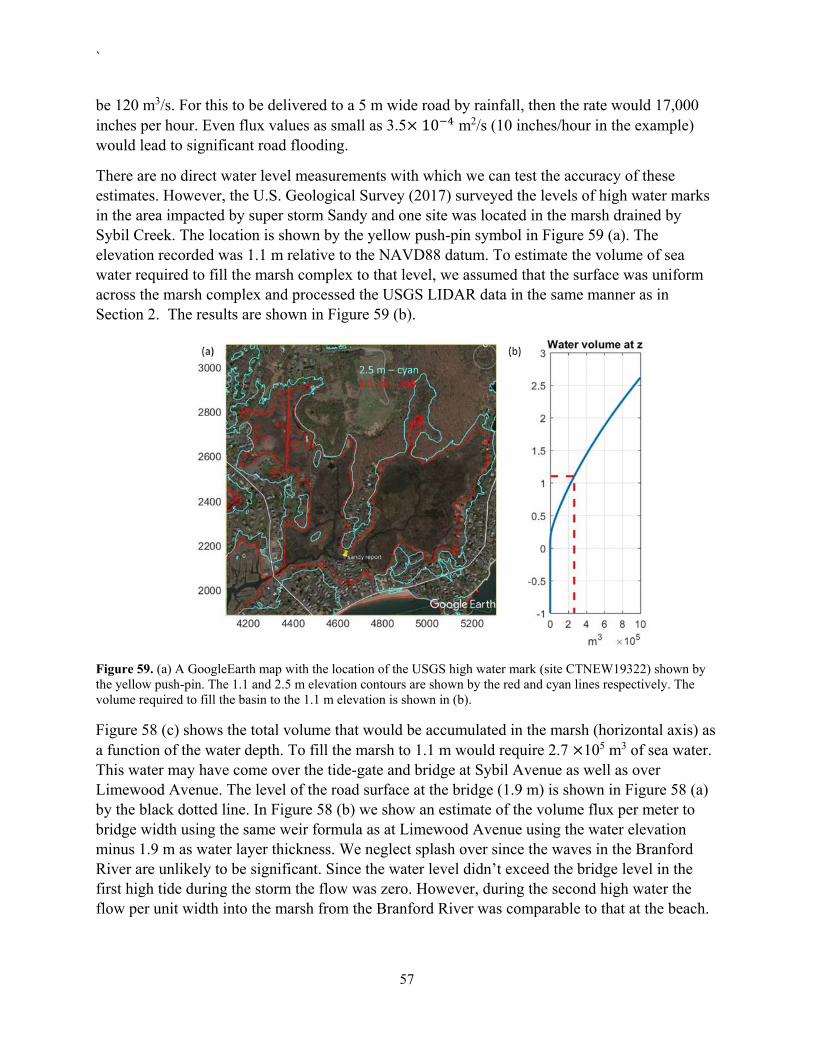
57  

be 120 m3/s. For this to be delivered to a 5 m wide road by rainfall, then the rate would 17,000 inches per hour. Even flux values as small as 3.5 10 m2/s (10 inches/hour in the example) would lead to significant road flooding.

There are no direct water level measurements with which we can test the accuracy of these estimates. However, the U.S. Geological Survey (2017) surveyed the levels of high water marks in the area impacted by super storm Sandy and one site was located in the marsh drained by Sybil Creek. The location is shown by the yellow push-pin symbol in Figure 59 (a). The elevation recorded was 1.1 m relative to the NAVD88 datum. To estimate the volume of sea water required to fill the marsh complex to that level, we assumed that the surface was uniform across the marsh complex and processed the USGS LIDAR data in the same manner as in Section 2. The results are shown in Figure 59 (b).

 

Figure 59. (a) A GoogleEarth map with the location of the USGS high water mark (site CTNEW19322) shown by the yellow push-pin. The 1.1 and 2.5 m elevation contours are shown by the red and cyan lines respectively. The volume required to fill the basin to the 1.1 m elevation is shown in (b).

Figure 58 (c) shows the total volume that would be accumulated in the marsh (horizontal axis) as a function of the water depth. To fill the marsh to 1.1 m would require 2.7 105 m3 of sea water. This water may have come over the tide-gate and bridge at Sybil Avenue as well as over Limewood Avenue. The level of the road surface at the bridge (1.9 m) is shown in Figure 58 (a) by the black dotted line. In Figure 58 (b) we show an estimate of the volume flux per meter to bridge width using the same weir formula as at Limewood Avenue using the water elevation minus 1.9 m as water layer thickness. We neglect splash over since the waves in the Branford River are unlikely to be significant. Since the water level didn’t exceed the bridge level in the first high tide during the storm the flow was zero. However, during the second high water the flow per unit width into the marsh from the Branford River was comparable to that at the beach.

` 

58  

To compare the contributions to the volume in the marsh we integrated the fluxes from both sources, the curves in Figure 58 (b), in time and assumed the flow across the beach occurred in a 50m wide swath and that the width for the flow across the bridge was 10m. In Figure 58 (c) we show the sum of the two volumes as the broad cyan line and the black line, and the black line with circles show the contributions form Limewood Avenue and the Sybil Avenue bridge. The latter is 16% of the flow over the beach.

The sum of the two fluxes is greater than the volume accumulated in the marsh as estimated from the USGS water level measurement. The ratio of the two values is 1.77. The red and the green lines in the Figure 58 (c) show the estimates of the volume transported into the marsh using the EurOtop II formulae but with 0.15 m added to the sea level observations. The lower value is 30 % larger than the estimate based on the high water mark and marsh geometry. Since we have assumed that the waves were approaching the beach from a normal angle, that the dissipation factors in the overtopping formula were unity, and that the wave height was at the maximum value for the entire storm, a high bias in our estimate is to be expected. Laudier et al. (2011) used a similar approach to calibrating the splash-over formula at a natural beach and found that the product of the 𝛾 coefficients in the range 0.64 to 0.72 produced estimates consistent with their observations. It is possible to refine this model further by carefully assessing the geometry and using the time evolution of the wave height from out model, however, the conclusions that a principle factor in the flooding of Sybil Creek marsh was the splash-over at Limewood Avenue, and that the risk of road flooding there can be usefully estimated by a simple model, are unlikely to change.

6.4 Analysis.

Using the link we have established between the water levels at Limewood and New Haven, then Figure 50 suggests that the mean water level has only exceeded the level of the road (2.3 m) once, during super storm Sandy, which created the highest storm surge in the available 18 year record. At the New London tide gage where the data record spans 80 years, super storm Sandy created the third highest water level. This suggest that at current mean sea level, flooding like that experienced in super storm Sandy has an annual probability in the range of 4% to 6%, or equivalently, a return interval in the range 18 to 26 years.

The risk of flooding on Limewood Avenue is much higher because of wave driven splash-over. The magnitude of the splash-over sea water volume flux is determined by the vertical distance between the mean water surface and the road level, the slope of the beach, and the significant wave height and period. Since the mean water level and significant wave height jointly determine the extent of flooding at Limewood Road, and around the Sybil Creek marsh, quantifying the risk requires estimation of the joint probability distribution. Since both waves and sea level are largely driven by wind the fluctuations are not independent. Estimation of the most appropriate probability distribution function requires further study.

The EurOtop II model can provide guidance on the range of conditions that will lead to significant flooding at Limewood Road. In Figure 60 we plot the estimated flux to Limewood Road per meter of shore front as a function of the sea level (the average over many waves) for a

` 

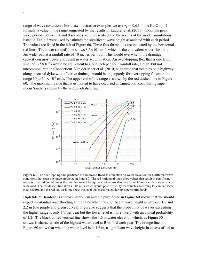
59  

range of wave conditions. For these illustrative examples we use γ 0.65 in the EurOtop II formula, a value in the range suggested by the results of Laudier et al. (2011). Example peak wave periods between 4 and 9 seconds were prescribed and the results of the model simulations listed in Table 2 were used to estimate the significant wave height associated with each period. The values are listed in the left of Figure 60. Three flux thresholds are indicated by the horizontal red lines. The lower (dotted) line shows 3.5 10-4 m2/s which is the equivalent water flux to a 5m wide road at a rainfall rate of 10 inches per hour. This would overwhelm the drainage capacity on most roads and result in water accumulation. An over-topping flux that is one tenth smaller (3.5 10-5) would be equivalent to a one inch per hour rainfall rate, a high, but not uncommon, rate in Connecticut. Van der Meer et al. (2010) suggested that vehicles on a highway along a coastal dyke with effective drainage would be in jeopardy for overtopping fluxes in the range 10 to 50 10-3 m3/s. The upper end of the range is shown by the red dashed line in Figure 60. The maximum value that is estimated to have occurred at Limewood Road during super storm Sandy is shown by the red dot-dashed line.

 

Figure 60. The over-topping flux predicted at Limewood Road as a function on water elevation for 6 different wave conditions that span the range predicted in Figure 7. The red horizontal lines show values that result in significant impacts. The red dotted line is the rate that would be equivalent to equivalent to a 10 inch/hour rainfall rate on a 5 m wide road. The red dashed line shows 0.05 m2/s which would pose difficulty for vehicles according to Van der Meer et al. (2010), and the red dot-dash line show the level that is estimated during super storm Sandy.

High tide at Branford is approximately 1 m and the purple line in Figure 60 shows that we should expect substantial road flooding at high tide when the significant wave height is between 1.8 and 2.2 m (the purple and green curves). Figure 56 suggests that the probability of waves exceeding the higher range is only 1/7 per year but the lower level is more likely with an annual probability of 1/2. The black dotted vertical line shows the 1.6 m water elevation which, as Figure 50 shows, is characteristic of the highest water level at Branford each year. The orange line in Figure 60 show that when the water level is at 1.6 m, a significant wave height in excess of 1.4 m

` 

60  

will result in significant water on the road surface. The figure also shows that a significant wave height of 1 m would produce a water flux comparable to a 1 inch per hour rain storm. The green and cyan lines show that the waves would need to be in excess of the conditions during super storm Sandy (1.9 m) for the vehicle hazard level to be exceeded during a “normal” storm.

The dependence of the overtopping fluxes on the wave conditions near high tide and in typical storm (one that should be expected each year) is demonstrated in Figure 61 (a) and (b), respectively. The intersection of the solid black curve and the red dotted line shows again that at high tide a 1.845 m significant wave height will result in severe road flooding. The intersections of the red dotted line with the black dashed, and dot-dashed lines are to the left indicating that at higher water levels, lower wave elevations (1.57 and 1.37 m) are required for splash-over to result in severe flooding. Figure 56 shows that the probability of waves in excess of 2 m is approximately 1/6.5 and that for 1.73 and 1.37 m are 1/4.8 and 1/38. It is plausible that by 2050 or 2100, the mean sea level could increase by 0.25 or 0.5 m. Assuming storm and wave statistics don’t change much over that time, then these relatively small changes in level would increase the risk of severe road flooding at high tide by approximately 134% to 172%.

 

Figure 61. (a) The dependence of the over-topping flux on the significant wave height (and period) at a typical high tide 𝜂 1 m) is shown by the solid black line. The variation at .25 and 0.5 m higher levels are shown by the dashed and dot-dashed lines respectively. The variation during high tide in a storm (𝜂 1.6 is shown in (b), where again the 0.25 and 0.5 m higher levels are shown by the dashed lines.

A similar analysis for the potential for severe flooding during high tide during normal storms can be developed using Figure 61 (b). At a sea level of 1.6 m (solid black curve) a significant wave height of 2.36 m leads to hazard level (red dashed line) flooding, however at 1.85 m and 2.1 m, significant wave heights of 1.90 and 1.38 m will have the same consequences. Note that the effect of the 0.25 and 0.5 m sea level change has a large impact on the change in wave height required to have the same flooding consequences at higher water levels because the first derivatives of the curves decrease at higher water levels and higher wave heights (they are flatter

` 

61  

on the right side of the graphs). The wave statistics in Figure 56 imply that the 2.36 m significant wave height has a probability of exceedance of 1/10.2 and that the smaller wave heights have probabilities of 1/6.9 and 1/2.7 respectively. Consequently, the increase in risk of hazard level flooding for .25 m and 0.5 m increases in sea level are 148% and 267%.

It is worthy of note that the substantial increase in risk predicted by the analysis is mainly due to two factors: the dependence of the over-topping flux on the water to road elevation separation, and the exponential shape of the wave exceedance diagram (Figure 56). Though the values reported above are estimates that are based on available data and models have uncertainty associated with them, the most important result (the substantial increase in the risk of flooding associated with small changes in mean sea level) are robust.

To evaluate the consequences of the combined effects of mean sea level changes on the flooding of the area around the Sybil Creek marsh, see Figure 19 (a), we repeated the calculations that led to Figure 15 but incrementally increased the mean sea level from 0 to 0.5 m in 0.05 m increments. We assumed that the sea level at New Haven was 0.15 m higher that Branford during the storm, and used a value of 𝛾 0.65 in the EurOtop II formula in to make the model

predictions more consistent with observations. We did not allow the significant wave height to evolve through the storm. We converted the predicted volume in the marsh using the relationship between volume and elevation computed from the LIDAR based topography and shown in Figure 59 (b). The black solid line in Figure 62 (b) shows the elevation in the marsh at the end of the simulated storm or when the elevation reached 2.5 m. At that catastrophic level the model of the flow into the marsh is not as reliable.

In Figure 62 (a) the green contour shows the 1.1 m contour which is the level of the high water mark surveyed and reported by the USGS (2017) in the Sybil Creek marsh to the east of the Sybil Avenue (RT 146) bridge and tide-gate. The blue line shows the 2.5 m level. This is a good estimate of the high water level during super storm Sandy. The area between the blue contour (2.5 m) and the red contour (1.1 m) were protected from flooding during super storm Sandy by the presence of the Sybil Creek marsh, the berm carrying Limewood Avenue (RT 146) and the tide-gate. The black line in Figure 62 (b) shows how a rise in the mean sea level will influence the maximum water level in in the area surrounding the marsh. A 0.28 m increase in the sea level is predicted to increase the high water level from 1.1 to 1.9 m and reduce the range of the elevations protected from flooding. The 1.9 m contour is shown in green in Figure 19 (a). Note that the .28 m increase in mean sea level leads to the high water level in the marsh areas increasing by 0.8m, a factor of 2.85 larger. This is rapid erosion of the flood protection value by rising sea level continues until at 0.42 m the high water level would reach 2.5 m. Worse still, areas that are between 2.5 and 2.92 m elevation would then be vulnerable to flooding.

` 

62  

 

Figure 62. (a) A GoogleEarth map of the coastal area near Limewood Avenue. The white line show the location of RT 146 and the red, green and blue lines show the 1.1 m 1.9, and 2.5 m elevation contours. (b) The black solid line shows the elevation in the marsh that corresponds to the maximum predicted volume transported into the marsh. The red dashed line shows the change in sea level in the marsh if it was just do to sea level rise.  

6.5 Summary

We have described the geography of the area of Branford between Limewood Avenue and the marsh surrounding Sybil Creek that is susceptible to coastal flooding. Using a combination of simple models of wave driven transport over the beach at Limewood, and the bridge at Sybil Avenue, we conclude that most of the flooding around the marsh during super storm Sandy was due to flow over the beach. Without an estimate of the joint probability of wave heights and sea level it is not possible to estimate the risk of future flooding adequately. This should be addressed in the future. However, the model allows us to assess what conditions would likely lead to flooding. At normal high tide levels, significant wave heights in the range of 1.37 to 1.57 m will lead to significant flooding on Limewood Avenue. During severe storm the high tide level increases to 1.6 m and significant wave heights in the range 1.0 to 1.5m will lead to substantial road flooding.

The models we developed also allow us to estimate the effects of sea level rise on the change in the risk of flooding in the area surrounding the Sybil Creek Marsh. It is clear that the land and properties are protected from high water by the tide gate and bridge at Sybil Creek, and by the berm that carries Limewood Avenue along the coast. When the water level in the Sound was 2.5 m during super storm Sandy, the water level in the marsh was only 1.1 m. Our model results show that an increase in sea level of 0.25 m allows flooding to 1.9 m, an increase of 0.8 m, and

` 

63  

shrinks the width of the flood protection zone from 1.4 m to 0.6 m. This rapid loss of flood risk protection is a robust characteristic of the model, especially at low sea level change values where the model is most reliable. The same analysis has the more positive result that small increases in the elevation of Limewood Avenue would reduce the flood risk considerably.

 

` 

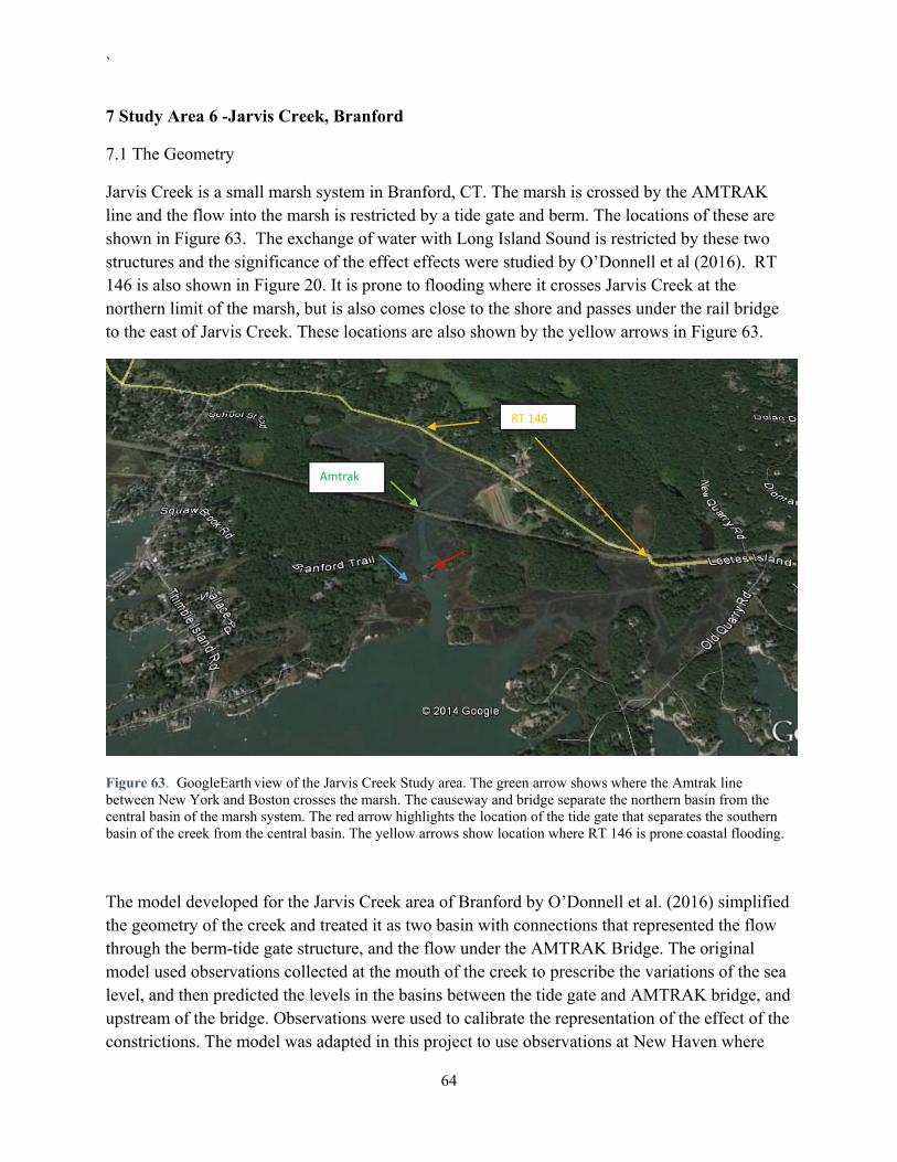
64  

7 Study Area 6 -Jarvis Creek, Branford

7.1 The Geometry

Jarvis Creek is a small marsh system in Branford, CT. The marsh is crossed by the AMTRAK line and the flow into the marsh is restricted by a tide gate and berm. The locations of these are shown in Figure 63. The exchange of water with Long Island Sound is restricted by these two structures and the significance of the effect effects were studied by O’Donnell et al (2016). RT 146 is also shown in Figure 20. It is prone to flooding where it crosses Jarvis Creek at the northern limit of the marsh, but is also comes close to the shore and passes under the rail bridge to the east of Jarvis Creek. These locations are also shown by the yellow arrows in Figure 63.

 

Figure 63. GoogleEarth view of the Jarvis Creek Study area. The green arrow shows where the Amtrak line between New York and Boston crosses the marsh. The causeway and bridge separate the northern basin from the central basin of the marsh system. The red arrow highlights the location of the tide gate that separates the southern basin of the creek from the central basin. The yellow arrows show location where RT 146 is prone coastal flooding.

The model developed for the Jarvis Creek area of Branford by O’Donnell et al. (2016) simplified the geometry of the creek and treated it as two basin with connections that represented the flow through the berm-tide gate structure, and the flow under the AMTRAK Bridge. The original model used observations collected at the mouth of the creek to prescribe the variations of the sea level, and then predicted the levels in the basins between the tide gate and AMTRAK bridge, and upstream of the bridge. Observations were used to calibrate the representation of the effect of the constrictions. The model was adapted in this project to use observations at New Haven where

Amtrak 

RT 146

` 

65  

measurements have been recorded since 1998 (see Figure 10). These elevations can then be used to characterize the future likelihood of flooding and the impact of the marsh and tide gates.

Figure 64 (a) shows the bathymetry and topography of the area surrounding Jarvis Creek using a color range chosen to clarify the variation between -1 m and 3 m. The red points show the locations on RT 146 where we used an RTK GPS survey system to measure the elevation of the road. In the area surrounded by the black dashed line, the road is prone to flooding near the bridge that crosses Jarvis Creek. The elevation measurements in this area are shown in Figure 64 (b) by the blue dots. The horizontal axis is the distance west from the eastern-most point and the dashed lines show the location of the bridge. There are two areas in this segment of the road that are at 1m elevation. Flow from Long Island Sound into this are of Jarvis Creek is restricted by the both the rail line and the tide gate. The red dashed line in Figure 64 (a) surrounds the area of where RT 146 goes under the AMTRAK line and Figure 64 (c) show the measurements of the road elevation on both sides of the underpass which is shown by the vertical dashed lines. The lowest point on the road in this are also at 1 m.

 

Figure 64. (a) The elevation and bathymetry in the range -1 to 3 m (NAVD88) in the vicinity Jarvis Creek. The red dots show the location on RT 146 where elevation measurements were made. (b) and (c) show the elevation measured at the locations of the red dots in the black and red squares respectively.

7.2 Model Simulations

The model of O’Donnell et al. (2016) was run using the parameters developed in the initial study but using the water levels measured at New Haven instead of those measure near the junction of Long Island Sound and Jarvis Creek. The forcing and the solution for the northern basin of the marsh is shown in Figure 65 (a) and (b) respectively. The 20 peaks that are heighted by the green circles are the largest anomalies separated in time by more than three days.

` 

66  

 

Figure 65. (a) The 17 year sea level record at New Haven which was used to force the model of Jarvis Creek to produce the predictions for the level in the northern basin that are shown in (b).

7.3 Analysis

The data and from New Haven and the simulation results in Figure 65 both show that the water levels are frequently above the 1.0 m level. There are several approaches to describe the frequency of flooding but most are designed to characterize the probability of infrequent events. In this area, flooding is frequent so we begin with an analysis of the tidal effects alone.

The underpass on RT 146, in the red square in Figure 64 (a), is adjacent to the entrance to Jarvis Creek and the water level that controls the flooding frequency is almost the same as at New Haven. In Figure 66 (a) we show the water level variation at New Haven due only to tidal forces between 1999 and 2016 by the blue points on the inset graph. We then examined the records and counted the number of days that the water level exceeded 1 m, and the duration of that day that the water was above the threshold. We then repeated the calculation for levels 1.1, 1.2, 1.3,….1.9, 2.0 m and show the average number of days per year that the water levels were above each of the thresholds in the lowest curve in Figure 66 (a). We find that water levels (due to tidal variations alone) will exceed 1 m on 5 days per year and it will not exceed 1.4 m. In Figure 66 (b) we show the average duration of the water level above the 1 m threshold to be 2 hours. We show a range of thresholds to allow evaluation of the consequences of the uncertainty associated with the leveling of the water level measurements which we estimate as 0.1 m. If the mean water level at Branford was 0.1 m lower than we estimate then flooding would not occur at the underpass until the 1.1. m level on the graph was exceeded and flooding would only be expected 2 days a year.

` 

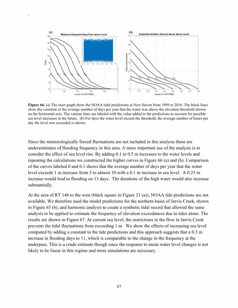
67  

 

Figure 66. (a) The inset graph show the NOAA tidal predictions at New Haven from 1999 to 2016. The black lines show the variation of the average number of days per year that the water was above the elevation threshold shown on the horizontal axis. The various lines are labeled with the value added to the predictions to account for possible sea level increases in the future. (b) For days the water level exceed the threshold, the average number of hours per day the level was exceeded is shown.

Since the meteorologically forced fluctuations are not included in this analysis these are underestimates of flooding frequency in this area. A more important use of the analysis is to consider the effect of sea level rise. By adding 0.1 to 0.5 m increases to the water levels and repeating the calculations we constructed the higher curves in Figure 66 (a) and (b). Comparison of the curves labeled 0 and 0.1 shows that the average number of days per year that the water level exceeds 1 m increase from 5 to almost 10 with a 0.1 m increase in sea level. A 0.25 m increase would lead to flooding on 13 days. The durations of the high water would also increase substantially.

At the area of RT 146 to the west (black square in Figure 21 (a)), NOAA tide predictions are not available. We therefore used the model predictions for the northern basin of Jarvis Creek, shown in Figure 65 (b), and harmonic analysis to create a synthetic tidal record that allowed the same analysis to be applied to estimate the frequency of elevation exceedances due to tides alone. The results are shown in Figure 67. At current sea level, the restrictions in the flow in Jarvis Creek prevents the tidal fluctuations from exceeding 1 m. We show the effects of increasing sea level computed by adding a constant to the tide predictions and this approach suggests that a 0.3 m increase in flooding days to 11, which is comparable to the change in the frequency at the underpass. This is a crude estimate though since the response to mean water level changes is not likely to be linear in this regime and more simulations are necessary.

` 

68  

 

Figure 67 (a) The black lines show the variation of the average number of days per year that the water was above the elevation threshold shown on the horizontal axis in the model of the northern basin of Jarvis Creek. The lines are labeled with the value added to the predictions to account for possible sea level increases in the future. (b) For days the water level exceed the threshold, the average number of hours per day the level was exceeded is shown.

A well-established technique to assess combined effect of meteorological and tidally forced variations is to use the “peak over threshold” (see Zervas, 2013) method. It assumes that the largest values in the record occur randomly with a Poisson distribution and that the magnitudes have a generalized Pareto distribution. Only independent peaks should be included in the analysis. We applied the approach to the two records shown in Figure 65. The peaks above 2.3 times the standard deviation of the series are identified by the green circles and the largest 20 peaks are indicated by arrows. The empirical cumulative distribution functions constructed from the peak over threshold series are shown in Figure 68. The blue diamond symbols show the elevation in the creek north of the tide gate. The red squares show values from Long Island Sound. Note that the levels between the AMTRAK bridge and the tide gate were indistinguishable from the blue symbols indicating that the railway bridge does not have much influence on water levels. The red squares tend to be higher and the difference between the red and blue-green trends is an indication of the effectiveness of the tide gate and marsh in reducing water levels at RT 146. Once the water level in the Sound exceeds 1.65m the peaks are all the same since the tide gate and marsh no longer have the effect of restricting the flow.

The colored lines are generalized extreme value function interpolants through the data. The fit for the two highest values (Hurricane Irene and Super Storm Sandy) is poor and extrapolation is unwise. Below 5 years, the observations and the empirical fit are in excellent agreement. Using either the interpolant or the observations, the analysis suggests that the roadway in the area of the would have to be elevated to 1.4 m to reduce the risk of flooding at the bridge (black square in the Figure 64) less than 1/year. The 1/year return interval level at the underpass (red square in Figure 21) is higher, 1.6 m. To reduce the flooding to once a decade a 2 m level would have to be achieved

` 

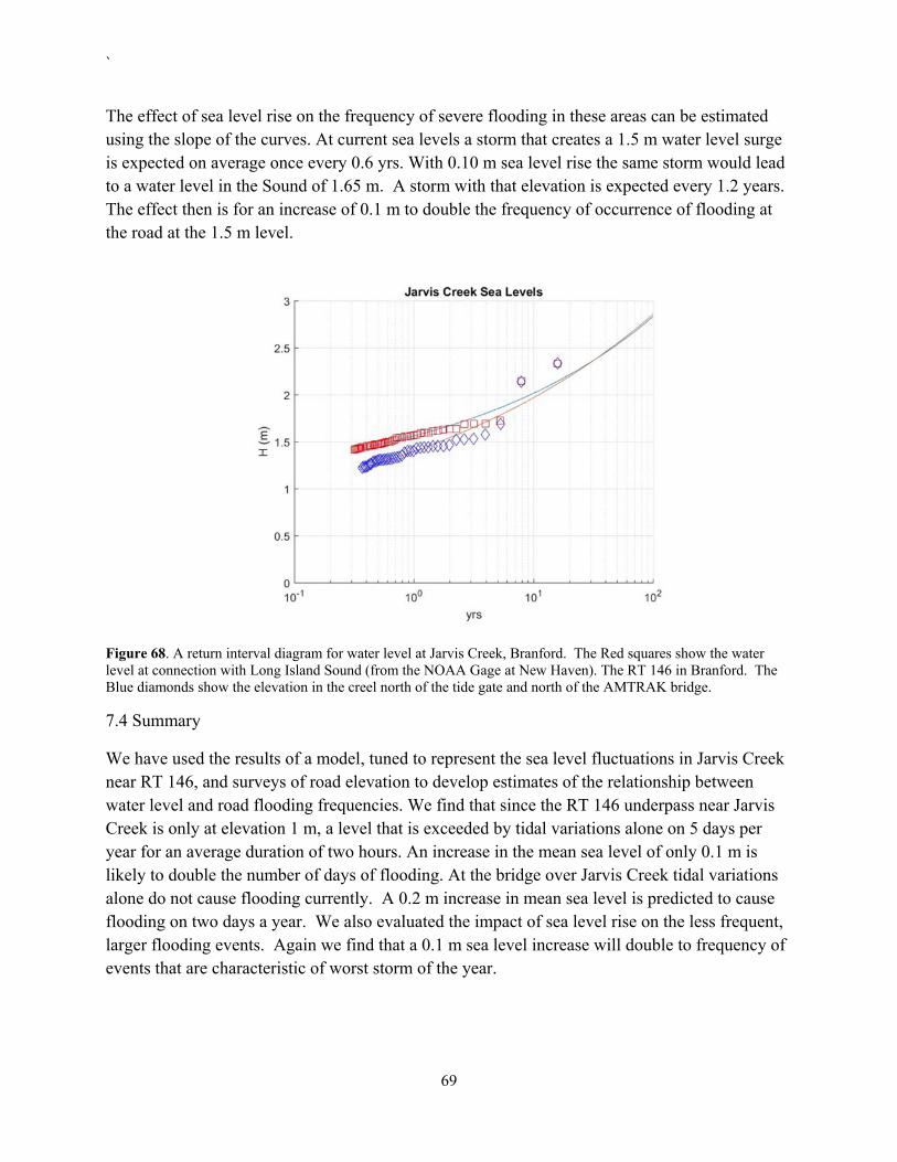
69  

The effect of sea level rise on the frequency of severe flooding in these areas can be estimated using the slope of the curves. At current sea levels a storm that creates a 1.5 m water level surge is expected on average once every 0.6 yrs. With 0.10 m sea level rise the same storm would lead to a water level in the Sound of 1.65 m. A storm with that elevation is expected every 1.2 years. The effect then is for an increase of 0.1 m to double the frequency of occurrence of flooding at the road at the 1.5 m level.

 

Figure 68. A return interval diagram for water level at Jarvis Creek, Branford. The Red squares show the water level at connection with Long Island Sound (from the NOAA Gage at New Haven). The RT 146 in Branford. The Blue diamonds show the elevation in the creel north of the tide gate and north of the AMTRAK bridge.

7.4 Summary

We have used the results of a model, tuned to represent the sea level fluctuations in Jarvis Creek near RT 146, and surveys of road elevation to develop estimates of the relationship between water level and road flooding frequencies. We find that since the RT 146 underpass near Jarvis Creek is only at elevation 1 m, a level that is exceeded by tidal variations alone on 5 days per year for an average duration of two hours. An increase in the mean sea level of only 0.1 m is likely to double the number of days of flooding. At the bridge over Jarvis Creek tidal variations alone do not cause flooding currently. A 0.2 m increase in mean sea level is predicted to cause flooding on two days a year. We also evaluated the impact of sea level rise on the less frequent, larger flooding events. Again we find that a 0.1 m sea level increase will double to frequency of events that are characteristic of worst storm of the year.

` 

70  

8. References

Chow, V.T. (1959) Open Channel Hydraulics. McGraw-Hill, 680pp.

Emery, W.J. and R.E. Thomson (2001). Data analysis methods in physical oceanography. 2nd Edt. Elsevier, Amsterdam. 638pp

Hughes, S.A. and N.C. Nadal (2009) Laboratory study of combined wave overtopping and storm surge overflow of a levee. Coastal Engineering 56(3):244-259. DOI: 10.1016/j.coastaleng.2008.09.005

Laudier, N.A., E.B. Thornton and J. MacMahan (2011) Measured and modeled wave overtopping on a natural beach. Coastal Eng., 58, 815-825

Linsley, R.K. and J. B. Franzini (1979) “Water-Resources Engineering”, 3rd.ed. Mcgraw-Hill, Blacklick, Ohio, U.S.A.

NOAA (2017a). https://tidesandcurrents.noaa.gov/datums.html?id=8465233 (accessed in

June, 2017)

NOAA (2017b). https://tidesandcurrents.noaa.gov/datums.html?id=8465748 (accessed in

June, 2017)

O’Donnell, J., M. Whitney, and M.M. Howard Strobel (2016). A Study of Coastal Flooding at Jarvis Creek, Connecticut. Technical Report to the Connecticut Department of Energy and Environmental Protection. https://www.researchgate.net/publication/311583802_A_Study_of_Coastal_Flooding_a

t_Jarvis_Creek_Connecticut?_iepl%5BviewId%5D=kft2ohsYoCTt9YbQRtCXSz5R&_iepl%5

BprofilePublicationItemVariant%5D=default&_iepl%5Bcontexts%5D%5B0%5D=prfpi&_i

epl%5BtargetEntityId%5D=PB%3A311583802&_iepl%5BinteractionType%5D=publicatio

nTitle

Roman, C.T., R.W. Garvine, and J.W. Portnoy. (1995). Hydrologic modeling as a predictive basis for ecological restoration of salt marshes. Environmental Management 19:559-566

USACE (2015). North Atlantic Coast Comprehensive Study: Resilient Adaptation to Increasing

Risk (http://www.nad.usace.army.mil/Portals/40/docs/NACCS/NACCS_main_report.pdf)  

USGS (2017). Topobathymetric Model for the New England Region States of New York, Connecticut, Rhode Island, and Massachusetts, 1887 to 2016 https://coast.noaa.gov/dataviewer/#/lidar/search/where:ID=6194 

U.S. Geological Survey (2017). Short-Term Network Data Portal, accessed on [June 25th, 2017], at http://water.usgs.gov/floods/FEV/

` 

71  

Van der Meer, J.W., T. Pullen, N.W.H. Allsop, T. Bruce, H. Schüttrumpf and A. Kortenhaus (2010). Prediction of overtopping. Chapter 14 in Handbook of Coastal and Ocean Engineering; Ed. Young C. Kim. World Scientific, pp. 341-382

Van der Meer, J.W., N.W.H. Allsop, T. Bruce, J. De Rouck, A. Kortenhaus, T. Pullen, H. Schüttrumpf, P. Troch, and B. Zanuttigh (2016). EurOtop II Manual on wave overtopping of sea defences and related structures: An overtopping manual largely based on European research, but for worldwide application (2nd Edt). http://www.overtopping-manual.com/docs/EurOtop II%20II%202016%20Pre-release%20October%202016.pdf

White, F.M. (2003) Fluid Mechanics (5th edt). McGraw-Hill, 866pp. ISBN 0-07-240217-2

Zervas, C. (2013) Extreme water levels of the United States 1893–2010. NOAA Technical Report NOSCO-OPS 067 (www.tidesandcurrents.noaa.gov/publications/NOAA_Technical_Report_NOS_COOPS_067a.pdf)