SCF algorithms for Hartree-Fockelectronic calculations�Eric CancèsCERMICS, Ecole Nationale des Ponts et Chaussées,6 & 8 avenue Blaise Pascal, Cité Descartes,F-77455 Marne-la-Vallée, France.cances@cermics.enpc.frNovember 26, 1999AbstractThis paper presents some mathematical results on SCF algorithms for solv-ing the Hartree-Fock problem. In the �rst part of the article the focus is on twoclassical SCF procedures, namely the Roothaan algorithm and the level-shiftingalgorithm. It is demonstrated that the Roothaan algorithm either converges to-wards a solution to the Hartree-Fock equations or oscillates between two stateswhich are not solution to the Hartree-Fock equations, any other behavior (os-cillations between more than two states, �chaotic� behavior, ...) being excluded.The level-shifting algorithm is then proved to converge for large enough shiftparameter, whatever the initial guess. The second part of the article details theconvergence properties of a new algorithm recently introduced by Le Bris andthe author, the so-called Optimal Damping Algorithm (ODA). Basic numericalsimulations pointing out the principal features of the various algorithms understudy are also provided.1 IntroductionThe Hartree-Fock (HF) model is a standard tool for computing an approximation ofthe ground state of a molecular system within the Born-Oppenheimer setting. Froma mathematical viewpoint, the HF model gives rise to a nonquadratic constrainedminimization problem for the numerical solution of which iterative procedures areneeded; such procedures are referred to as Self-Consistent Field (SCF) algorithms.The solution to the HF problem can be obtained either by directly minimizing theHF energy functional [7, 12, 18, 26] or by solving the associated Euler-Lagrangeequations, the so-called Hartree-Fock equations [21, 22, 23].SCF algorithms for solving the HF equations are in general much more e�cientthan direct energy minimization techniques. However, these algorithms do not apriori ensure the decrease of the energy and they may lead to convergence problems[24]. For instance, the famous Roothaan algorithm (see [22] and section 4) is knownto sometimes lead to stable oscillations between two states, none of them being asolution to the HF problem. This situation may occur even for simple chemicalsystems (see section 4).Many articles have been devoted to the important issue of the SCF convergence.The behavior of the Roothaan algorithm is notably investigated in [2, 13] and in�To appear in Mathematical models and methods for ab initio Quantum Chemistry, M. De-franceschi and C. Le Bris (Eds.), in preparation for Lecture Notes in Chemistry, Springer.1

[27, 28]. In [2, 13] convergence di�culties are demonstrated for elementary two-dimensional models; in [27, 28], a stability condition of the Roothaan algorithm in theneighbourhood of a minimum of the HF energy is given for closed-shell systems. Moresophisticated SCF algorithms for solving the HF equations have also been proposed toimprove the convergence using various techniques like for instance damping [11, 29]or level-shifting [23]. Damping (as implemented in [29]) cures some convergenceproblems but many other remain. Numerical tests con�rm that the level-shiftingalgorithm converges towards a solution to the HF equations for large enough shiftparameters; a perturbation argument is provided in [23] to prove this convergence inthe neighborhood of a stationary point. Unfortunately there is no guarantee that theso-obtained critical point of the HF energy functional is actually a minimum (evenlocal); in addition, the level-shifting algorithm is known to only o�er a slow speed ofconvergence. In practice, the most commonly used SCF algorithm is at the presenttime the Direct Inversion in the Iteration Space (DIIS) algorithm [21]. Numericaltests show that this algorithm is very e�cient in most cases, but that it sometimesfails.The present article belongs to a series of articles [3, 4, 5] devoted to the SCF algo-rithms.Our �rst purpose here is to report on recent mathematical results on the convergenceproperties of the Roothaan and of the level-shifting algorithms. Section 4 concernsthe Roothaan algorithm, which is the most �natural� algorithm for solving the HFequations. Its is demonstrated that the Roothaan algorithm either converges towardsa solution to the HF equations or oscillates between two states which are not solutionto the HF equations, any other behavior being excluded. This theoretical result isin accordance with the numerical experiments. It is then explained in Section 5 whythe introduction of a �level-shift� makes the algorithm converge. The mathematicalproofs are presented in the context of the �nite dimension approximations of the HFproblem obtained by a Galerkin method with a �nite basis of atomic orbitals or planewaves, typically. They are consequently much simpler from a technical viewpointthan the proofs detailed in [3] which concern the original in�nite dimension HFproblem.Recently, new SCF algorithms has been introduced in [4] by Le Bris and the author.They seem to exhibit good convergence properties at least for the chemical systemscomputed so far. These algorithms have been called Relaxed Contraints Algorithms(RCA) for they can be interpretated as direct minimization procedure of the HFenergy which do not care about satisfying at each iteration the nonlinear constraintsD2 = D that characterize admissible density matrices. The second purpose of thisarticle (section 6) is to detail the mathematical proof of the convergence of thebasic RCA, namely the Optimal Damping Algorithm (ODA). Section 6 also containssome comments on the connexions between RCA and other algorithms like the level-shifting and the DIIS algorithms.Before coming up to our main topic, we devote section 2 to a brief presentationof the HF model for readers (especially mathematicians) who are not familiar withQuantum Chemistry. Section 3 collects various general comments that apply to allthe SCF algorithms considered in the sequel.2 A brief presentation of the Hartree-Fock modelThe problem under consideration consists in computing ab initio, that is to saywithout using any empirical parameter, the ground state energy of a molecular system2

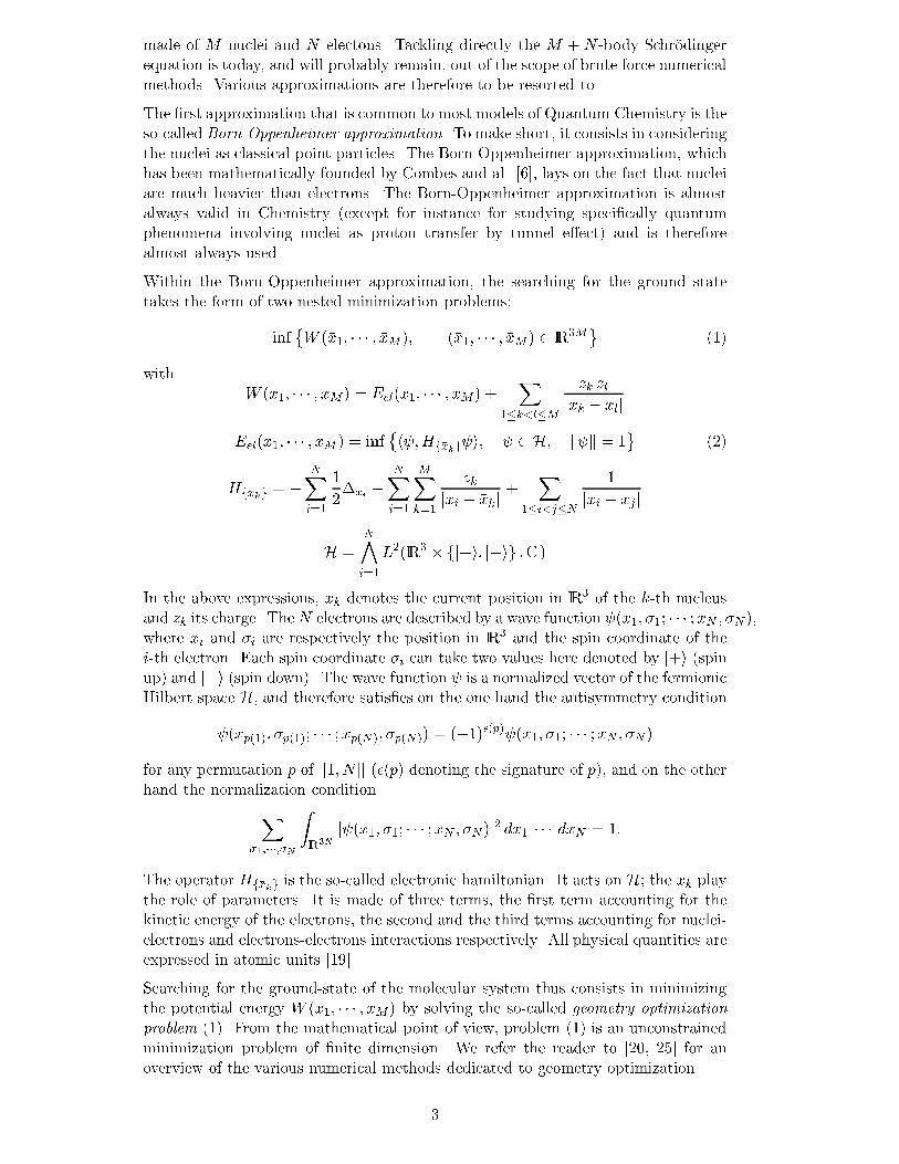
made of M nuclei and N electons. Tackling directly the M + N -body Schrödingerequation is today, and will probably remain, out of the scope of brute force numericalmethods. Various approximations are therefore to be resorted to.The �rst approximation that is common to most models of Quantum Chemistry is theso-called Born-Oppenheimer approximation. To make short, it consists in consideringthe nuclei as classical point particles. The Born-Oppenheimer approximation, whichhas been mathematically founded by Combes and al. [6], lays on the fact that nucleiare much heavier than electrons. The Born-Oppenheimer approximation is almostalways valid in Chemistry (except for instance for studying speci�cally quantumphenomena involving nuclei as proton transfer by tunnel e�ect) and is thereforealmost always used.Within the Born-Oppenheimer approximation, the searching for the ground statetakes the form of two nested minimization problems:inf �W (�x1; � � � ; �xM ); (�x1; � � � ; �xM ) 2 IR3M (1)with W (�x1; � � � ; �xM ) = Eel(�x1; � � � ; �xM ) + X1�k<l�M zk zlj�xk � �xljEel(�x1; � � � ; �xM ) = inf �h ;Hf�xkg i; 2 H; k k = 1 (2)Hf�xkg = � NXi=1 12�xi � NXi=1 MXk=1 zkjxi � �xkj + X1�i<j�N 1jxi � xjjH = N̂i=1L2(IR3 � fj+i; j�ig ;Cj )In the above expressions, �xk denotes the current position in IR3 of the k-th nucleusand zk its charge. TheN electrons are described by a wave function (x1; �1; � � � ;xN ; �N ),where xi and �i are respectively the position in IR3 and the spin coordinate of thei-th electron. Each spin coordinate �i can take two values here denoted by j+i (spinup) and j�i (spin down). The wave function is a normalized vector of the fermionicHilbert space H, and therefore satis�es on the one hand the antisymmetry condition (xp(1); �p(1); � � � ;xp(N); �p(N)) = (�1)�(p) (x1; �1; � � � ;xN ; �N )for any permutation p of j[1; N ]j (�(p) denoting the signature of p), and on the otherhand the normalization conditionX�1;���;�N ZIR3N j (x1; �1; � � � ;xN ; �N )j2 dx1 � � � dxN = 1:The operator Hf�xkg is the so-called electronic hamiltonian. It acts on H; the �xk playthe role of parameters. It is made of three terms, the �rst term accounting for thekinetic energy of the electrons, the second and the third terms accounting for nuclei-electrons and electrons-electrons interactions respectively. All physical quantities areexpressed in atomic units [19].Searching for the ground-state of the molecular system thus consists in minimizingthe potential energy W (�x1; � � � ; �xM ) by solving the so-called geometry optimizationproblem (1). From the mathematical point of view, problem (1) is an unconstrainedminimization problem of �nite dimension. We refer the reader to [20, 25] for anoverview of the various numerical methods dedicated to geometry optimization.3

The speci�city of problem (1) is that the function to be minimized, namely the poten-tial energy W , is itself the result (up to the internuclear repulsion termP zkzl=j�xk��xlj) of the minimization problem (2) which is usally referred to as the electronic prob-lem. We face this time a constrained minimization problem on the in�nite dimensionspace H.In the sequel, we focus on the electronic problem, which is rewritten (in order tosimplify the notations) inf fh ;H i; 2 H; k k = 1g (3)with H = N̂i=1L2(IR3 � fj+i; j�ig ;Cj )H = � NXi=1 12�xi + NXi=1 V (xi) + X1�i<j�N 1jxi � xjjV (x) = � MXk=1 zkjx� �xkjthe �xk being now �xed parameters in IR3.The Hartree-Fock approximation is of variational nature. It consists in restrictingthe set f 2 H; k k = 1g on which the energy functional h ;H i is minimized tothe set of the Slater determinants, i.e. to the set of the wave functions of the form = 1pN ! det(�i(xj ; �j)) (4)where the �i, which are called molecular orbitals, satisfy the orthonormality condi-tions X� ZIR3 �i(x; �)�j(x; �)� dx = �ij :A classical calculation (see [19] for instance) gives for any of the form (4)h ;H i = EHF (f�ig)with EHF (f�ig) = NXi=1 12 ZIR3X� jr�ij2 + ZIR3 �� V+12 ZIR3 ZIR3 ��(x) ��(x0)jx� x0j dx dx0�12 ZIR3 ZIR3X�;�0 j��(x; �;x0; �0)j2jx� x0j dx dx0;��(x; �;x0; �0) = NXi=1 �i(x; �)�i(x0; �0)�;��(x) = NXi=1X� j�i(x; �)j2:4

The HF problem thus readsinf(EHF (f�ig); �i 2 L2(IR3 � fj+i; j�ig ;Cj ); X� ZIR3 �i(x; �)�j(x; �)� dx = �ij) :The mathematical properties of the HF problem have been studied by Lieb andSimon [15] and by P.-L. Lions [16]. The existence of a HF electronic ground state isguaranteed for positive ions (Z :=PMk=1 zk > N) and neutral systems (Z = N). Weare not aware of any general existence result for negative ions (the available existenceproofs only work for N < Z+1). On the other hand, there is a non-existence resultsfor negative ions such that N > 2Z +M [14] (this inequality holds for instance forthe ion H2�). As far as we know, uniqueness (of the density � at least) is an openproblem, probably of outstanding di�culty.The last step of the approximation procedure consists in approaching the in�nitedimensional HF problem by a �nite dimensional HF problem by means of a Galerkinapproximation: the HF energy is minimized over the set of molecular orbitals thatcan be expanded on a given �nite basis f�pg1�p�n:�i = nXk=1Cki�k:Denoting by S = [Skl] with Skl =X� ZIR3 ��k�lthe so-called overlap matrix, the contraints X� ZIR3 �i��j = �ij read�ij =X� ZIR3 �i��j =X� ZIR3 nXl=1 Cli�l! nXk=1Ckj�k!� = nXk=1 nXl=1 C�kjSklCli;or in matricial form C�SC = IN ;where IN denotes the identity matrix of rank N . In addition,NXi=1 12 ZIR3 jr�ij2 + ZIR3 �� V = NXi=1 �12 ZIR3 jr�ij2 + ZIR3 V j�ij2�= NXi=10@12 ZIR3 �����r nXk=1Cik�k�����2 + ZIR3 V ����� nXk=1Cik�k�����21A= NXi=1 nXk=1 nXl=1 hklCliC�ki= Tr (hCC�)where h denotes the matrix of the core hamiltonian �12�+ V in the basis f�kg:hkl = 12X� ZIR3 r��k � r�l +X� ZIR3 V ��k�l:Lastly, denoting by(ijjkl) =X� X�0 ZIR3 ZIR3 �i(x)�j(x)��k(x0)�l(x0)�jx� x0j dx dx0 and Aijkl = (ijjkl)�(iljkj);5

the interelectronic repulsion term readsZIR3 ZIR3 ��(x) ��(x0)jx� x0j dx dx0�ZIR3 ZIR3 j��(x; x0)j2jx� x0j dx dx0 = nXi;j;k;l=1 NX�;�=1AijklCi�C�j�Ck�C�l�:The above expressions incite one to introduce the so-called density matrixD = CC�;which permits to write the HF energy under the compact formEHF (D) = Tr (hD) + 12Tr (G(D)D);where G(D) denotes the contracted product of the 4-index tensor A by D:G(D)ij = (A : D)ij =Xkl AijklDkl:It is easy to see that the matrices D which read D = CC� with C 2 M(n;N) andC�SC = IN are those which satisfy Tr (SD) = N and DSD = D. The so-obtained�nite dimension HF problem then readsinf �EHF (D); D 2M(n; n); D� = D; Tr (SD) = N; DSD = D :For the sake of simplicity, we assume in the sequel that the overlap matrix S equalsidentity, that is to say that the basis f�pg1�p�n is orthonormal. The general case isrecovered by the transformation rules D ! S1=2DS1=2, h! S�1=2hS�1=2, G(D)!S�1=2G(S1=2DS1=2)S�1=2. The HF problem then reads:inf �EHF (D); D 2 P ; (5)with P = �D 2M(n; n); D� = D; Tr D = N; D2 = D :The following lemma provides a characterization of the critical points of the HFminimization problem (5).Lemma 1. For any D, let us denote by F (D) = h+G(D) the Fock matrix associatedwith D.1. A density matrix D 2 P is a critical point of the HF problem (5) if and only if8<: F (D)C = CEC�C = IND = CC� (6)where E = Diag(�1; �2; � � � ; �N ) is a N �N diagonal matrix collecting N eigen-values of the linear eigenvalue problemF (D) � � = � �:and where C is a n �N matrix containing N orthonormal eigenvectors asso-ciated with �1, �2, ..., �N . The condition (6) is equivalent to the condition[F (D);D] = 0;where [�; �] denotes the matrix commutator de�ned for any A and B in M(n; n)by [A;B] = AB �BA. 6

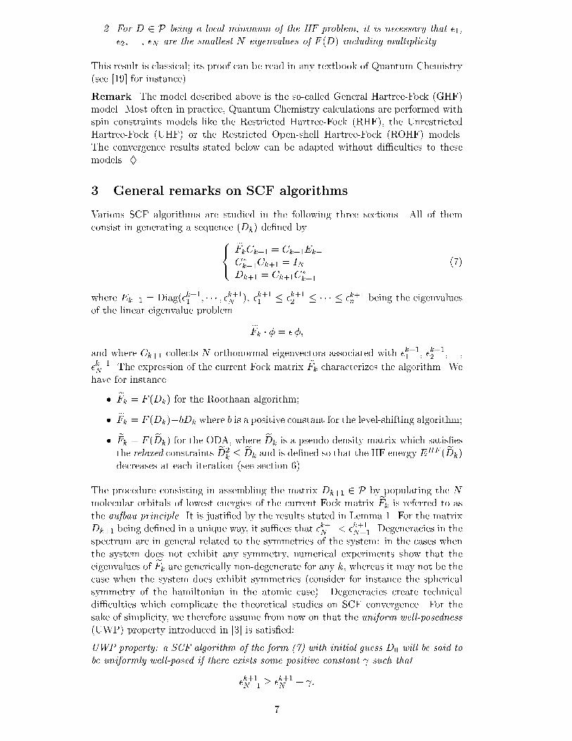
2. For D 2 P being a local minimum of the HF problem, it is necessary that �1,�2, ..., �N are the smallest N eigenvalues of F (D) including multiplicity.This result is classical; its proof can be read in any textbook of Quantum Chemistry(see [19] for instance).Remark. The model described above is the so-called General Hartree-Fock (GHF)model. Most often in practice, Quantum Chemistry calculations are performed withspin constraints models like the Restricted Hartree-Fock (RHF), the UnrestrictedHartree-Fock (UHF) or the Restricted Open-shell Hartree-Fock (ROHF) models.The convergence results stated below can be adapted without di�culties to thesemodels. }3 General remarks on SCF algorithmsVarious SCF algorithms are studied in the following three sections. All of themconsist in generating a sequence (Dk) de�ned by8<: eFkCk+1 = Ck+1Ek+1C�k+1Ck+1 = INDk+1 = Ck+1C�k+1 (7)where Ek+1 = Diag(�k+11 ; � � � ; �k+1N ), �k+11 � �k+12 � � � � � �k+1n being the eigenvaluesof the linear eigenvalue problem eFk � � = � �;and where Ck+1 collects N orthonormal eigenvectors associated with �k+11 , �k+12 , ...,�k+1N . The expression of the current Fock matrix eFk characterizes the algorithm. Wehave for instance� eFk = F (Dk) for the Roothaan algorithm;� eFk = F (Dk)�bDk where b is a positive constant for the level-shifting algorithm;� eFk = F ( eDk) for the ODA, where eDk is a pseudo-density matrix which satis�esthe relaxed constraints eD2k � eDk and is de�ned so that the HF energy EHF ( eDk)decreases at each iteration (see section 6).The procedure consisting in assembling the matrix Dk+1 2 P by populating the Nmolecular orbitals of lowest energies of the current Fock matrix eFk is referred to asthe aufbau principle. It is justi�ed by the results stated in Lemma 1. For the matrixDk+1 being de�ned in a unique way, it su�ces that �k+1N < �k+1N+1. Degeneracies in thespectrum are in general related to the symmetries of the system: in the cases whenthe system does not exhibit any symmetry, numerical experiments show that theeigenvalues of eFk are generically non-degenerate for any k, whereas it may not be thecase when the system does exhibit symmetries (consider for instance the sphericalsymmetry of the hamiltonian in the atomic case). Degeneracies create technicaldi�culties which complicate the theoretical studies on SCF convergence. For thesake of simplicity, we therefore assume from now on that the uniform well-posedness(UWP) property introduced in [3] is satis�ed:UWP property: a SCF algorithm of the form (7) with initial guess D0 will be said tobe uniformly well-posed if there exists some positive constant such that�k+1N+1 � �k+1N + :7

The consequences of the UWP assumption which will be useful below have beencollected in the following lemma, whose proof is postponed until the end of thepresent section.Lemma 2. Let us consider a SCF algorithm of the form (7) with initial guess D0which satis�es the UWP property. Then1. The updated density matrix Dk+1 is de�ned in a unique way at each iteration;this matrix can be characterized as the minimizer of the variational probleminf nTr ( eFkD); D 2 Po :2. For any D 2M(n; n) such that D = D�, Tr (D) = N and D2 � D,Tr ( eFkD) � Tr ( eFkDk+1) + 2 kD �Dk+1k2;k � k denoting the Hilbert-Schmidt norm de�ned for any A 2M(n; n) by kAk =Tr (AA�)1=2.In the sequel, we denote by arg inf MP the minimizer of the minimization problemMP . We can therefore writeDk+1 = arg inf nTr ( eFkD); D 2 Po :Remark. Let us point out that some convergence results can be obtained withoutresorting to the UWP assumption. In particular, it turns out that the level-shiftingalgorithm is automatically UWP as soon as the shift parameter is large enough (see [3]for details). It can also be proved that the ODA numerically converges towards anaufbau solution to the HF equations within the GHF setting and provided the basis is�large enough�. We do not detail here the rather technical proof of this assertion. Letus just mention that it is based on a mathematical result by P.-L. Lions [17] relatedto �nite-temperature HF models. Unfortunately, so far as we know, the argumentsused in [17] cannot be extended to the RHF, UHF or ROHF models. }Before turning to the study of SCF algorithms, the notion of convergence has to bemade precise. We are in fact not able to prove mathematical convergence results ofthe form �the sequence (Dk) converges towards a minimizer D of the HF problem(5)� for at least two reasons. First, we are solving the Euler-Lagrange equationsassociated with the HF minimization problem (5), namely the HF equations (6);even in case of convergence we have no argument to conclude that the so-obtainedcritical point is actually a minimum (even local) of the HF energy. Second, we haveno precise description of the topology of the set of the critical points of (5); this lackof information prevents us from proving the convergence of the whole sequence (Dk)towards a solution D to the HF equations. We can at best obtain that Dk+1 �Dkgoes to zero, and that for �large� k, Dk is �close to� a solution to the HF equations(6) satisfying the aufbau principle. For instance, it may happen that the HF problemadmits a connected manifold of minima; this phenomenon is observed in particularfor open-shell atoms because the spherical symmetry of the problem is broken by theHF approximation (this can be related to a mathematical result by Bach, Lieb, Lossand Solovej [1] stating that �there are no un�lled shell� in the HF ground states).We cannot then discriminate between the case when the sequence (Dk) convergestowards a point of the manifold and the case when the sequence (Dk) is attractedby the manifold together with a slow drift parallel to the manifold.8

We shall consequently adopt here the following two convergence criteria, which aresu�cient in practice. We shall say that a SCF algorithm of the form (7) numericallyconverges towards a solution to the HF equations if the sequence (Dk) satis�es1. Dk+1 �Dk �! 0;2. [F (Dk);Dk] �! 0;and that it numerically converges towards an aufbau solution to the HF equations ifthe sequence (Dk) satis�es1. Dk+1 �Dk �! 0;2. Tr (F (Dk)Dk)� inf fTr (F (Dk)D); D 2 Pg �! 0.As all norms are equivalent in �nite dimension, we do not need to specify the matrixnorm in which the variations are evaluated. Let us remark that the latter convergencecriterion is stronger than the former one for(Tr (F (Dk)Dk)� inf fTr (F (Dk)D); D 2 Pg ! 0) ) ([F (Dk);Dk]! 0) :Let us conclude this section with theProof of Lemma 2. Let us denote by D a current matrix such that D = D�, Tr (D) =N , D2 � D and by Dij its coe�cients in an orthonormal basis in which eFk =Diag(�k+11 ; �k+12 ; � � � ; �k+1n ) with �k+11 � �k+12 � � � � � �k+1n . In such a basis Dk+1 =Diag(1; � � � ; 1; 0; � � � ; 0). As in addition Tr (D) =Pni=1Dii = N , we get �rstkDk+1 �Dk2 = Tr ((Dk+1 �D) � (Dk+1 �D))= Tr �D2k+1�+Tr �D2�� 2Tr (DDk+1)� Tr (Dk+1) + Tr (D)� 2Tr (DDk+1)= 2N � 2 NXi=1 Dii= 2 nXi=N+1Dii:Besides Tr ( eFkDk+1) =PNi=1 �k+1i , Tr ( eFkD) =Pni=1 �k+1i Dii and0 � Dii � 1; for any 1 � i � nfor D2 � D = D� implies jDiij2 +Pj 6=i jDij j2 � Dii. Putting together the aboveresults, we obtainTr ( eFkD) = nXi=1 �k+1i Dii� NXi=1 �k+1i Dii + nXi=N+1(�k+1N + )Dii= NXi=1 �k+1i Dii + �k+1N nXi=N+1Dii + nXi=N+1Dii= NXi=1 �k+1i Dii + �k+1N (N � NXi=1 Dii) + nXi=N+1Dii= NXi=1 �k+1i + NXi=1(�k+1N � �k+1i )(1 �Dii) + nXi=N+1Dii:9

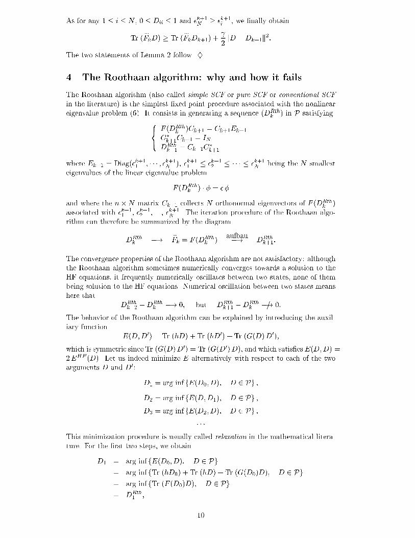
As for any 1 � i � N , 0 � Dii � 1 and �k+1N � �k+1i , we �nally obtainTr ( eFkD) � Tr ( eFkDk+1) + 2 kD �Dk+1k2:The two statements of Lemma 2 follow. }4 The Roothaan algorithm: why and how it failsThe Roothaan algorithm (also called simple SCF or pure SCF or conventional SCFin the literature) is the simplest �xed point procedure associated with the nonlineareigenvalue problem (6). It consists in generating a sequence (DRthk ) in P satisfying8<: F (DRthk )Ck+1 = Ck+1Ek+1C�k+1Ck+1 = INDRthk+1 = Ck+1C�k+1where Ek+1 = Diag(�k+11 ; � � � ; �k+1N ), �k+11 � �k+12 � � � � � �k+1N being the N smallesteigenvalues of the linear eigenvalue problemF (DRthk ) � � = � �and where the n�N matrix Ck+1 collects N orthonormal eigenvectors of F (DRthk )associated with �k+11 , �k+12 , ..., �k+1N . The iteration procedure of the Roothaan algo-rithm can therefore be summarized by the diagramDRthk �! eFk = F (DRthk ) aufbau�! DRthk+1:The convergence properties of the Roothaan algorithm are not satisfactory: althoughthe Roothaan algorithm sometimes numerically converges towards a solution to theHF equations, it frequently numerically oscillates between two states, none of thembeing solution to the HF equations. Numerical oscillation between two states meanshere that DRthk+2 �DRthk �! 0; but DRthk+1 �DRthk �!= 0:The behavior of the Roothaan algorithm can be explained by introducing the auxil-iary function E(D;D0) = Tr (hD) + Tr (hD0) + Tr (G(D)D0);which is symmetric since Tr (G(D)D0) = Tr (G(D0)D), and which satis�esE(D;D) =2EHF (D). Let us indeed minimize E alternatively with respect to each of the twoarguments D and D0: D1 = arg inf fE(D0;D); D 2 Pg ;D2 = arg inf fE(D;D1); D 2 Pg ;D3 = arg inf fE(D2;D); D 2 Pg ;� � �This minimization procedure is usually called relaxation in the mathematical litera-ture. For the �rst two steps, we obtainD1 = arg inf fE(D0;D); D 2 Pg= arg inf fTr (hD0) + Tr (hD) + Tr (G(D0)D); D 2 Pg= arg inf fTr (F (D0)D); D 2 Pg= DRth1 ; 10

and, since E is symmetric on P � P,D2 = arg infnE(D;DRth1 ); D 2 Po= arg infnE(DRth1 ;D); D 2 Po= arg infnTr (hD) + Tr (hDRth1 ) + Tr (G(DRth1 )D); D 2 Po= arg infnTr (F (DRth1 )D); D 2 Po= DRth2 :It follows by induction that the sequences generated by the relaxation algorithm onthe one hand, and by the Roothaan algorithm on the other hand, are the same.The functional E, which decreases at each iteration of the relaxation procedure cantherefore be interpreted as a Lyapunov functional of the Roothaan algorithm. Thisbasic remark is the foundation of the proof of the following result.Theorem 1. Let D0 2 P such that the Roothaan algorithm with initial guess D0 isUWP. Then the sequence (DRthk ) generated by the Roothaan algorithm satis�es oneof the following two properties� either (DRthk ) numerically converges towards an aufbau solution to the HF equa-tions� or (DRthk ) numerically oscillates between two states, none of them being anaufbau solution to the HF equations.Proof. For any k 2 IN, we deduce from Lemma 2 thatTr (F (DRthk+1)DRthk+2) + 2 kDRthk+2 �DRthk k2 � Tr (F (DRthk+1)DRthk ):Adding Tr (hDRthk+1) to both terms of the above inequality, we obtainE(DRthk+1;DRthk+2) + 2 kDRthk+2 �DRthk k2 � E(DRthk ;DRthk+1):We then sum up the above inequalities for k 2 IN and we getPk2IN kDRthk+2�DRthk k2 <+1, which involves in particular thatDRthk+2 �DRthk �! 0:Now, either DRthk+1 �DRthk converges to zero or it does not. In the former case, wededuce from the characterization of DRthk+1 byTr (F (DRthk )DRthk+1) = inf nTr (F (DRthk )D); D 2 Pothat Tr (F (DRthk )DRthk )� inf nTr (F (DRthk )D); D 2 Po �! 0:Convergence towards an aufbau solution to the HF equations is thus established. Inthe latter caseTr (F (DRth2k )DRth2k )� inf nTr (F (DRth2k )D); D 2 Po = Tr (F (DRth2k )DRth2k )� Tr (F (DRth2k )DRth2k+1)� 2 kDRth2k �DRth2k+1k2 �!= 0:11

Convergence of (D2k) towards an aufbau solution to the HF equations is thereforeexcluded; the same argument holds for (D2k+1). }Mimicking the proof of Theorem 2 (see section 5), it is easy to establish in additionthat (D2k;D2k+1) converges up to an extraction to a critical point (D;D0) 2 P �Pof the functional E which satis�es8>>>>>><>>>>>>:F (D0)C = CEC�C = IND = CC�F (D)C 0 = C 0E0C 0�C 0 = IND0 = C 0C 0�where E and E0 are diagonal matrices collecting the smallest N eigenvalues of F (D0)amd F (D) respectively. Besides, as E(D2k;D2k+1) is decreasing, the whole sequence(D2k; D2k+1) converges to (D;D0) if this critical point is a strict (local) minimum.In this case, the alternatives are� either (D;D0) is on the diagonal of P �P (i.e. D = D0) and (DRthk ) convergestowards an aufbau solution to the HF equations;� or (D;D0) is not on the diagonal of P �P (i.e. D 6= D0) and (DRthk ) oscillatesbetween two states which are not aufbau solutions to the HF equations.Both situations are represented on Figure 1.D0 D = D0

D(D0; D1) (D2; D1)(D2; D3)D0 D = D0(D0; D1) (D2; D1)(D2; D3)D

Figure 1: Minimization of E by relaxation: convergence towards a strict local mini-mum located on (resp. o�) the �diagonal� leads to the convergence (resp. oscillations)of the Roothaan algorithm.Oscillations can be observed even for simple chemical systems. As a matter of exam-ple, we have tested the Roothaan algorithm in the UHF setting for the atoms of theperidic table and for two sets of atomic orbitals, namely the gaussian basis sets 3-21Gand 6-311++G(3df,3pd) (see [10]). The initial guess is obtained by diagonalizationof the core hamiltonian. Calculations have been performed with Gaussian 98 [9].The results are reported in Figure 2; they indicate that1. Both alternatives (convergence vs oscillation) are met in practice.12

2. Convergence towards a critical point of the HF problem which is not a globalminimum can sometimes be observed.3. For the same system, we can get convergence for one basis set and oscillationfor another basis set.Base = 3-21G Base = 6-311++G(3df,3pd)

Convergence towards a solution to the HF equations which may be the HF ground state

Convergence towards a solution to the HF equations which is not the HF ground state

Oscillation between two states

Basis not available in Gaussian 98Figure 2: Searching the ground state of atoms with the Roothaan algorithm. Resultsare shown on the periodic table of the elements.5 Level-shiftingThe analysis developed in the previous section suggests to add to the functional Ea penalization term Ep of the o�-diagonal pairs (D;D0) with D 6= D0 in order toenforce the critical points of the functional E +Ep to lie on the diagonal of P � P,which should ensure convergence towards a critical point of (5).A simple penalization fonctional reads Ep = bkD�D0k2, where b is a positive constantand where k � k denotes as above the Hilbert-Schmidt norm. Let us therefore setEb(D;D0) = Tr (hD) + Tr (hD0) + Tr (G(D)D0) + b kD �D0k2:The relaxation algorithm associated with the minimization probleminf nEb(D;D0); (D;D0) 2 P � Pogenerates the sequence (Dbk) de�ned byDbk �! eFk = F (Dbk)� bDbk aufbau�! Dbk+1:The sequence (Dbk) can be identi�ed with the sequence generated by the so-calledlevel-shifting algorithm [23] with level-shift parameter b. The convergence of the13

level-shifting algorithm towards a (non necessarily aufbau) solution to the HF equa-tions is mathematically guaranteed:Theorem 2. There exists a positive constant b0 such that for any D0 2 P and forany level-shift parameter b � b0,1. The sequence of the energies EHF (Dbn) decreases towards some stationary valueE of EHF .2. The sequence (Dbn) numerically converges towards a solution to the HF equa-tions.Proof. Let b0 be a positive constant such that8(D;D0) 2M(n; n)�M(n; n); Tr �G(D �D0) � (D �D0)� � b0kD �D0k2: (8)Such a b0 exists since (d; d0) 7! Tr (G(d)d0) is a bilinear form on M(n; n). As Eb issymmetric on P � P, we have for any k 2 IN,Eb(Dbk;Dbk+1) = inf nEb(Dbk;D); D 2 Po� Eb(Dbk;Dbk):A simple calculation shows that this inequality can be rewritten asEHF (Dbk+1)� 12Tr (G(Dbk+1 �Dbk) � (Dbk+1 �Dbk)) + bkDbk+1 �Dbkk2 � EHF (Dbk):Therefore, for any b � b0,EHF (Dbk+1) + b2kDbk+1 �Dbkjj2 � EHF (Dbk): (9)It follows that (EHF (Dbk)) is a decreasing sequence and that+1Xk=0 kDbk+1 �Dbkjj2 < +1:The latter statement, which has been obtained by summing the inequalities (9) fork � 0, implies in particular that Dbk+1 �Dbk �! 0:As for any k 2 IN, [F (Dbk)� bDbk;Dbk+1] = 0;it follows that [F (Dbk);Dbk] = [F (Dbk)� bDbk;Dbk+1 �Dbk] �!k!+1 0:This concludes the proof of statement 2. As P is compact, we can extract from(Dbk)k2IN a subsequence (Dbkl)l2IN which converges towards some D 2 P, such thatEHF (Dbkl) # EHF (D) and [F (D);D] = 0; E = limEHF (Dk) = EHF (D) is thereforea stationary value of the HF energy. }The level-shift parameter b0 implicitely de�ned by (8) is far from being optimal.Explicit and more re�ned estimates of shift parameters that garantee convergenceare given in [3]. From a numerical viewpoint, it is important to choose not too large14

a shift parameter; otherwise the speed of convergence is very slow and the risk ofconverging towards a critical point whose energy is above that of the HF ground stateis enhanced. This point, on which we will come back in the course of section 6, isillustrated by the numerical example reported on Figure 3 in which the level-shiftingalgorithm with various shift parameters has been used to compute the (doublet)UHF ground state of the Bromine atom in the gaussian basis 6-311++G(3df,3pd)(see [10]). In each case, the initial guess is computed by diagonalizing the corehamiltonian. Calculations have been performed with Gaussian 98 [9]. The algorithmoscillates for small shift parameters. For larger shift parameters, damped oscillationsleading to convergence are observed. For very large shift parameter, the energydecreases at each iteration. Too large shift parameters have however to be excludedbecause they slow down the convergence (for b = 30:0 Ha, convergence towards theground state is obtained after more than 200 iterations).

Iterations

HF

ene

rgy

0 10 20 30 40 50 60

-2500

-2550

-2450

Roothaan algorithmHF ground state

Iterations

HF

ene

rgy

0 10 20 30 40 50 60

-2500

-2550

-2450

LS with b = 1.1 HaHF ground state

Iterations

HF

ene

rgy

0 10 20 30 40 50 60

-2500

-2550

-2450

LS with b = 1.2 HaHF ground state

Iterations

HF

ene

rgy

0 10 20 30 40 50 60

-2500

-2550

-2450

LS with b = 1.5 HaHF ground state

Iterations

HF

ene

rgy

0 10 20 30 40 50 60

-2500

-2550

-2450

LS with b = 5.0 HaHF ground state

Iterations

HF

ene

rgy

0 10 20 30 40 50 60

-2500

-2550

-2450

LS with b = 30.0 HaHF ground state

Figure 3: Calculation of the UHF ground state of the Bromine atom.15

6 The Optimal Damping AlgorithmThe present section is devoted to the mathematical study of the Optimal Damp-ing Algorithm (ODA) which is the simplest representative of the class of RelaxedConstraints Algorithms (RCA) introduced in [4].The ODA is de�ned by the following two-step iteration procedure1. Diagonalize the current Fock matrix eFk = F ( eDk) and assemble the matrixDk+1 2 P by the aufbau principle;2. Set eDk+1 = arg infnE( eD); eD 2 Seg[ eDk;Dk+1]o whereSeg[ eDk;Dk+1] = n(1� �) eDk + �Dk+1; � 2 [0; 1]odenotes the line segment linking eDk and Dk+1.The procedure is initialized with eD0 = D0, D0 2 P being a given initial guess.The ODA thus generates two sequences of matrices:� The principal sequence of density matrices (Dk)k2IN which will be proved tonumerically converge towards an aufbau solution to the HF equations;� A secondary sequence ( eDk)k�1 of pseudo-density matrices which belong to theset eP = n eD 2M(n; n); eD� = eD; Tr ( eD) = N; eD2 � eDoobtained from P by relaxing the nonlinear constraints D2 = D.The latter statement is a direct consequence ofLemma 3. The set P is convex,whose proof is postponed until the end of the present section. Indeed, eD0 = D0 2P � eP and, by induction, if eDk 2 eP then by convexity eDk+1 2 Seg[ eDk;Dk+1] � ePsince Dk+1 2 P � eP.The properties of the ODA are put together in the following theorem.Theorem 3. For any initial guess D0 for which the ODA is UWP,1. The sequence E( eDk) decreases towards a stationary value of the HF energy.2. The sequence (Dk)k2IN converges towards an aufbau solution to the HF equa-tions.As a �rst step towards the understanding of the ODA, let us consider eDk 2 eP andD0 2 P, and let us compute the variation of the HF energy on the line segmentSeg[ eDk;D0] = n(1� �) eDk + �D0; � 2 [0; 1]o :We obtain for any � 2 [0; 1],EHF ((1��) eDk+�D0) = EHF ( eDk)+�Tr (F ( eDk)�(D0� eDk))+�22 Tr �G(D0 � eDk) � (D0 � eDk)� :The �steepest descent� direction, i.e. the density matrix D for which the slopes eDk!D = Tr (F ( eDk) � (D � eDk)) is minimum, is given by the solution to the mini-mization problemD = arg infnTr (F ( eDk) � (D0 � eDk)); D0 2 Po ;16

which also reads D = arg infnTr (F ( eDk) �D0); D0 2 Po :This is precisely the direction Dk+1 obtained by the aufbau principle. The ODAcan therefore be interpretated as a steepest descent algorithm in eP . The practicalimplementation of the ODA is detailed in [4] for the RHF setting. The cost ofone ODA iteration is approximatively the same as the cost of one iteration of theRoothaan algorithm (see [4] for details).Figure 4 reports on a comparison between the ODA and the DIIS approaches forthe calculation of the RHF ground state of the E form of n-methyl-2-nitrovinylamine(CH3-NH-CH=CH-NO2) in the basis 6-31G(d) (see [8]). The speed of convergenceis estimated by computing the logarithm of the di�erence between the HF energy ofthe current density matrix and the (presumed) HF ground state energy. Calculationshave been performed within Gaussian 98 [9]. The graph on the left hand side corre-sponds to an initial guess computed by a semiempirical method. In this case, bothalgorithms converge but the speed of convergence of the DIIS algorithm is higher.From a general viewpoint, numerical tests performed until now demonstrate that theODA is e�cient for performing the early iterations of the SCF procedure; when thesequence (Dk) has reached a neighbourhood of a critical point of the HF problem,convergence can be accelerated either by resorting to iterative subspace techniquesor by switching to a quadratically convergent algorithm [4]. On the other hand, onlythe ODA converges for a more crude initial guess obtained by diagonalizing the corehamiltonian, as illustrated by the graph on the right hand side.

CPU time (s)

Err

or o

n th

e en

ergy

(lo

g)

0 10.5 1.5

-10

0

-5

ODA DIIS

CPU time (s)

Err

or o

n th

e en

ergy

(lo

g)

0 1 2 3 4 5 6

-10

0

-5

ODA DIISFigure 4: A comparison between the ODA and the DIIS algorithms: search for theRHF ground state of the E form of n-methyl-2-nitrovinylamine with an initial guessobtained by a semiempirical method (on the left hand side) and with the initial guessobtained by diagonalizing the core hamiltonian (on the right hand side).Let us now detail theProof of Theorem 3. Let us denote by eFk = F ( eDk) and by sk+1 = Tr ( eFk(Dk+1 �eDk)). In view of Lemma 2,sk+1 = Tr � eFkDk+1�� Tr � eFk eDk� � � 2 kDk+1 � eDkk2:As above, let us denote by b0 a positive constant such that8( eD; eD0) 2M(n; n)�M(n; n); Tr �G( eD0 � eD) � ( eD0 � eD)� � b0k eD � eD0k2:17

For any � 2 [0; 1],EHF ((1� �) eDk + �Dk+1) � EHF ( eDk)� 2 kDk+1 � eDkk2�+ b02 kDk+1 � eDkk2�2:ThereforeEHF ( eDk+1) = inf nEHF ((1� �) eDk + �Dk+1); � 2 [0; 1]o� inf�EHF ( eDk)� 2 kDk+1 � eDkk2�+ b02 kDk+1 � eDkk2�2; � 2 [0; 1]�= EHF ( eDk)� �kDk+1 � eDkk2with � = 2=8b0 if � 2b0, � = ( � b0)=2 otherwise. We then add up the aboveinequalities for k 2 IN, and we get P kDk+1 � eDkk2 < +1, which implies thatDk+1 � eDk �! 0: (10)As eDk+1 2 [ eDk;Dk+1], it follows thateDk+1 � eDk �! 0;and then that Dk+1 �Dk �! 0:Besides Tr (F ( eDk)Dk+1) = inf nTr (F ( eDk)D); D 2 Po : (11)Putting together (10) and (11), we �nally obtainTr (F (Dk+1)Dk+1)� inf fTr (F (Dk+1)D); D 2 Pg �! 0: }The following two points discuss the links between RCA and other algorithms likethe level-shifting and the DIIS algorihms.The �rst point concern the level-shifting algorithm. Let us use the ODA to minimizethe penalized energy functionalEb(D) = EHF (D)� b2Tr (D2):As for any D 2 P, Tr (D2) = Tr (D) = N , the critical points of the minimizationproblem inf nEb(D); D 2 Po (12)are the same as those of the HF problem (5). On the other hand, for any eD 2 eP nP,Tr (D2) < N : �interior� points are penalized. Let us denote by (Dbk) and ( eDbk) thesequences generated by the ODA algorithm applied to (12):1. Diagonalize the current Fock matrix eF bk = F ( eDbk) � b eDbk and assemble thematrix Dbk+1 2 PN by the aufbau principle;2. Set eDbk+1 = arg infnE( eD); eD 2 Seg[ eDbk;Dbk+1]o.18

As for any � 2 [0; 1]Eb((1� �) eDbk + �Dbk+1) = Eb( eDbk) + �Tr ( eF bk � (Dk+1 � eDk))+�22 �Tr �G(Dbk+1 � eDbk) � (Dbk+1 � eDbk)�� bkDbk+1 � eDbkk2� ;we obtain sk+1 = Tr ( eF bk � (Dk+1 � eDk)) � � 2kDbk+1 � eDbkk2and for b � b0Tr �G(Dbk+1 � eDbk) � (Dbk+1 � eDbk)�� bkDbk+1 � eDbkk2 � 0:For b � b0, the function � 7! Eb((1 � �) eDbk + �Dbk+1) is therefore decreasing andconcave on [0; 1]; it follows that eDbk+1 = Dbk+1 which means that the ODA for min-imizing (12) coincides with the level-shi�ng algorithm. This provides in particularanother proof of the convergence of the level-shifting algorithm for large shift pa-rameters b. Now, if Db is an accumulation point of the sequence (Dbk), we obtain bypassing to the limits1 = inf nTr ((F (Db)� bDb) � (D �Db)); D 2 Po = 0:This implies thatDb = arg infnTr ((F (Db)� bDb) �D); D 2 Po ;and therefore that [F (Db)� bDb;Db] = [F (Db);Db] = 0;but not necessarily that Db = arg inf�Tr (F (Db)D); D 2 P: Db is a solution tothe HF equations that may not satisfy the aufbau principle. In addition, as G(D) � 0for any D 2 P, we obtainsk+1 = Tr ( eF bk � (Dbk+1 �Dbk))= Tr (F (Dbk) � (Dbk+1 �Dbk)) + b2kDbk+1 �Dbkk2� �2 jinf fTr (hD); D 2 Pgj+ b2kDbk+1 �Dbkk2:It results that kDbk+1 �Dbkk2 � 2b jinf fTr (hD); D 2 Pgj :The level-shifting algorithm can then also be interpreted as a trust region algorithmon the manifold P for which the radius of the trust region is bounded by � =2b jinf fTr (hD); D 2 Pgj. The larger the shift parameter b, the smaller the stepDbk+1 �Dbk; this induces for large b a slow motion along a steepest descent path.The second point is related to the DIIS algorithm. An attempt of improvement of theODA consists, in the spirit of iterative subspace methods, in keeping in memory all(or some of) the density matrices computed at the previous steps and in minimizingthe HF energy in the convex set generated by all the density matrices stored inmemory:1. Diagonalize F ( eDk) and assemble the density matrix Dk+1 2 P by the aufbauprinciple . 19

2. Set eDk+1 = arg inf(EHF ( eD); eD = k+1Xi=0 ciDi; 0 � ci � 1; k+1Xi=0 ci = 1).This algorithm is similar to Pulay's DIIS algorithm [21] except that in the DIISalgorithm, step 2 consists in minimizing the residual k+1Xi=0 ci[F (Di);Di] 2 ; (13)where [:; :] denotes the commutator [A;B] = AB �BA, and where k � k denotes theHilbert-Schmidt norm. Contrary to the RCA presented here, the DIIS algorithmmay diverge: the residual (13) actually decreases at each step but it may vanishwithout the convergence is met.Let us conclude this section with theProof of Lemma 3. Let eD1 2 P and eD2 2 P. For any 0 � c1; c2 � 1 such thatc1 + c2 = 1, eD2 = (c1 eD1 + c2 eD2)2= c21 eD21 + c22 eD22 + c1c2( eD1 eD2 + eD2 eD1)= c1 eD1 + c2 eD2 + c1( eD21 � eD1) + c2( eD22 � eD2)+(c21 � c1) eD21 + (c22 � c2) eD22 + c1c2( eD1 eD2 + eD2 eD1)= eD + c1( eD21 � eD1) + c2( eD22 � eD2)� c1c2( eD1 � eD2)2since c21 � c1 = c1(1� c1) = �c1c2 = c22 � c2. Now, eD21 � eD1 � 0, eD22 � eD2 � 0 and( eD1 � eD2)2 � 0. Consequently, eD2 � eD. The other two constraints ( eD = eD� andTr ( eD) = N) being linear, it is clear that eD 2 eP . }References[1] V. Bach, E.H. Lieb, M. Loss and J.P. Solovej, There are no un�lled shells inunrestricted Hartree-Fock theory, Phys. Rev. Letters 72 (1994) 2981-2983.[2] V. Bona�ci¢-Koutecký and J. Koutecký, General properties of the Hartree-Fockproblem demonstrated on the frontier orbital model. II. Analysis of the customaryiterative procedure, Theoret. Chim. Acta 36 (1975) 163-180.[3] E. Cancès and C. Le Bris, On the convergence of SCF algorithms for the Hartree-Fock equations, to appear in Math. Model. Num. Anal.[4] E. Cancès and C. Le Bris, Can we outperform the DIIS approach for electronicstructure calculations, Int. J. Quantum Chem., submitted.[5] E. Cancès and C. Le Bris, An e�cient strategy to solve a nonlinear eigenvalueproblem issued from electronic calculations in Quantum Chemistry, J. Comput.Phys., submitted.[6] J.-M. Combes, P. Duclos and R. Seiler, The Born-Oppenheimer approximation,in Rigorous atomic and molecular physics, G. Velo and A. Wightman (Eds),Plenum Press 1981.[7] R. Fletcher, Optimization of SCF LCAO wave functions, Mol. Phys. 19 (1970)55-63. 20

[8] J.B. Foresman and A. Frisch, Exploring chemistry with electronic structure meth-ods, 2nd edition, Gaussian Inc., Pittsburgh PA 1996.[9] M.J. Frisch, G.W. Trucks, H.B. Schlegel, G.E. Scuseria, M.A. Robb, J.R.Cheeseman, V.G. Zakrzewski, J.A. Montgomery, R.E. Stratmann, J.C. Burant,S. Dapprich, J.M. Millam, A.D. Daniels, K.N. Kudin, M.C. Strain, O. Farkas, J.Tomasi, V. Barone, M. Cossi, R. Cammi, B. Mennucci, C. Pomelli, C. Adamo, S.Cli�ord, J. Ochterski, G.A. Petersson, P.Y. Ayala, Q. Cui, K. Morokuma, D.K.Malick, A.D. Rabuck, K. Raghavachari, J.B. Foresman, J. Cioslowski, J.V. Or-tiz, B.B. Stefanov, G. liu, A. Liashenko, P. Piskorz, I. Kpmaromi, G. Gomperts,R.L. Martin, D.J. Fox, T. Keith, M.A. Al-Laham, C.Y. Peng, A. Nanayakkara,C. Gonzalez, M. Challacombe, P.M.W. Gill, B.G. Jpohnson, W. Chen, M.W.Wong, J.L. Andres, M. Head-Gordon, E.S. Replogle and J.A. Pople, Gaussian98 (Revision A.7), Gaussian Inc., Pittsburgh PA 1998.[10] A. Frisch and M.J. Frisch, Gaussian 98 user's reference, Gaussian Inc., Pitts-burgh PA 1999.[11] D.R. Hartree, The calculation of atomic structures, Wiley 1957.[12] A. Igawa and H. Fukutome, A new direct minimization algorithm for Hartree-Fock calculations, Prog. Theor. Phys. 54 (1975) 1266-1281.[13] J. Koutecký and V. Bona�ci¢, On convergence di�culties in the iterative Hartree-Fock procedure, J. Chem. Phys. 55 (1971) 2408-2413.[14] E.H. Lieb, Bound on the maximum negative ionization of atoms and molecules,Phys. Rev. A 29 (1984) 3018-3028.[15] E.H. Lieb and B. Simon, The Hartree-Fock theory for Coulomb systems, Com-mun. Math. Phys. 53 (1977) 185-194.[16] P.-L. Lions, Solutions of Hartree-Fock equations for Coulomb systems, Comm.Math. Phys. 109 (1987) 33-97.[17] P.-L. Lions, Hartree-Fock and related equations, Nonlinear partial di�erentialequations and their applications, Collège de France Seminar Vol. 9 (1988) 304-333.[18] R. McWenny, The density matrix in self-consistent �eld theory I. Iterative con-struction of the density matrix, Proc. R. Soc. London Ser. A 235 (1956) 496-509.[19] R. McWenny, Methods of molecular Quantum Mechanics, Academic Press 1992.[20] A. Neumaier, Molecular modeling of proteins and mathematical prediction ofprotein structure, SIAM Rev. 39 (1997) 407-460.[21] P. Pulay, Improved SCF convergence acceleration, J. Comp. Chem. 3 (1982)556-560.[22] C.C.J. Roothaan, New developments in molecular orbital theory, Rev. Mod.Phys. 23 (1951) 69-89.[23] V.R. Saunders and I.H. Hillier, A "level-shifting" method for converging closedshell Hartree-Fock wave functions, Int. J. Quantum Chem. 7 (1973) 699-705.[24] H.B. Schlegel and J.J.W. McDouall, Do you have SCF stability and convergenceproblems?, in Computational Advances in Organic Chemistry, Kluwer Academic,1991, 167-185. 21

[25] T. Schlick, Optimization methods in computational chemistry, in Reviews inComputational Chemistry, Vol. III, K.B. Lipkowitz and D.B. Boyd (Eds.), VCHPublishers 1992.[26] R. Seeger R. and J.A. Pople, Self-consistent molecular orbital methods. XVI.Numerically stable direct energy minimization procedures for solution of Hartree-Fock equations, J. Chem. Phys. 65 (1976) 265-271.[27] R.E. Stanton, The existence and cure of intrinsic divergence in closed shell SCFcalculations, J. Chem. Phys. 75 (1981) 3426-3432.[28] R.E. Stanton, Intrinsic convergence in closed-shell SCF calculations. A generalcriterion, J. Chem. Phys. 75 (1981) 5416-5422.[29] M.C. Zerner and M. Hehenberger, A dynamical damping scheme for convergingmolecular SCF calculations, Chem. Phys. Letters 62 (1979) 550-554.

22