SE 207: Modeling and SimulationUnit 1

Introduction to Modeling and Simulation

Dr. Samir Al-AmerTerm 072

Unit Contents and ObjectivesLesson 1: IntroductionLesson 2: Classification of Systems

Unit 1 Objectives:To give an overview of the course (Modeling & simulation). Define important terminologies Classify systems/models

SE 207: Modeling and SimulationUnit 1

Introduction to Modeling and Simulation

Lecture 1: Introduction

Reading Assignment: Chapter 1 (Sections 1.1, 1.2)

SystemsWhat is a system?

SystemsA system is any set of interrelated components acting together to achieve a common objective.

Definition covers systems of different typesSystems vary in size, nature, function, complexity,…Boundaries of the system is determined by the scope of the studyCommon techniques can be used to treat them

ExamplesBattery

Consists of anode, cathode, acid and other components These components act together to achieve one objective

Car Electrical systemConsists of a battery, a generator, lamps,…achieve a common objective

SAPTCO (transportation company)Consists of Buses, drivers, stations,…Achieves a common objective

The Boundaries of the system is determined by the scope of the study

SystemsA system is any set of interrelated components acting together to achieve a common objective.

inputs system outputs

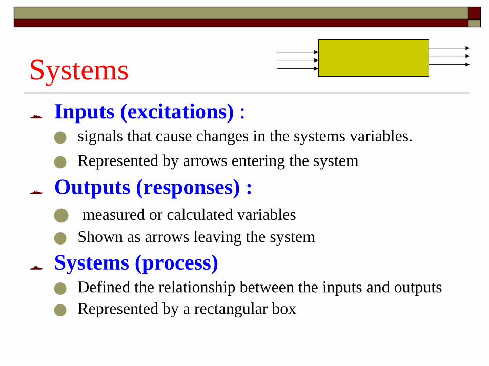
SystemsInputs (excitations) :

signals that cause changes in the systems variables.Represented by arrows entering the system

Outputs (responses) :measured or calculated variables

Shown as arrows leaving the system

Systems (process)Defined the relationship between the inputs and outputsRepresented by a rectangular box

The choice of inputs/outputs/process depends on the purpose of the study

Some Possible InputsInlet flow rateTemperature of entering materialConcentration of entering material

Some Possible OutputsLevel in the tankTemperature of material in tankOutlet flow rateConcentration of material in tank

What inputs and outputs are needed when we want to model the temperature of the water in the tank?

Modeling and SimulationModeling:

Obtain a set of equations (mathematical model) that describes the behavior of the system

A model describes the mathematical relationship between inputs and outputs

Simulation: Use the mathematical

model to determine the response of the system in different situations.

Falling Ball ExampleA ball falling from a height of 100 meters

We need to determine a mathematical model that describe the behavior of the falling ball.

Objectives of the model: answer these questions:1. When does the ball reach ground?2. What is the impact speed?

Different assumptions results in different models

Falling Ball ExampleCan you list some of the assumptions?

Falling Ball ExampleAssumptions for Model 1

1. Initial position = 100 x(0) = 1002. Initial speed = 0 v(0) = 03. Location: near sea level4. The only force acting on the ball is the

gravitational force (no air resistance)

ttvttx

Solution

8.9)()8.9(5.0100)(

:2

−=−=

0)0(;100)0(

)(;8.9

:

==

=−=

vx

tvdtdx

dtdvModel

Falling Ball ExampleSimulation of Model 1

The ball reaches ground at t = 4.5175 velocity = − 44.2719

Falling Ball ExampleMore models

Other mathematical models are possible. One such model includes the effect of air resistance. Here the drag force is assumed to be proportional to the square of the velocity.

0)0(;100)0(

)(;8.9

:2coeffient drag theis , resistanceair

2

2

==

=+−=

=

vx

tvdtdxv

mc

dtdvModel

cwherecv

How far can this stunt driver jump?

List some assumptions for solving this problem

Stunt driverAssumptions:

Point mass Mass of car+driver =MInitial speed = v0

Angle of inclination =aNo drag force

Model can be obtained to give the distance covered by the jump in terms of M,a, v0,…

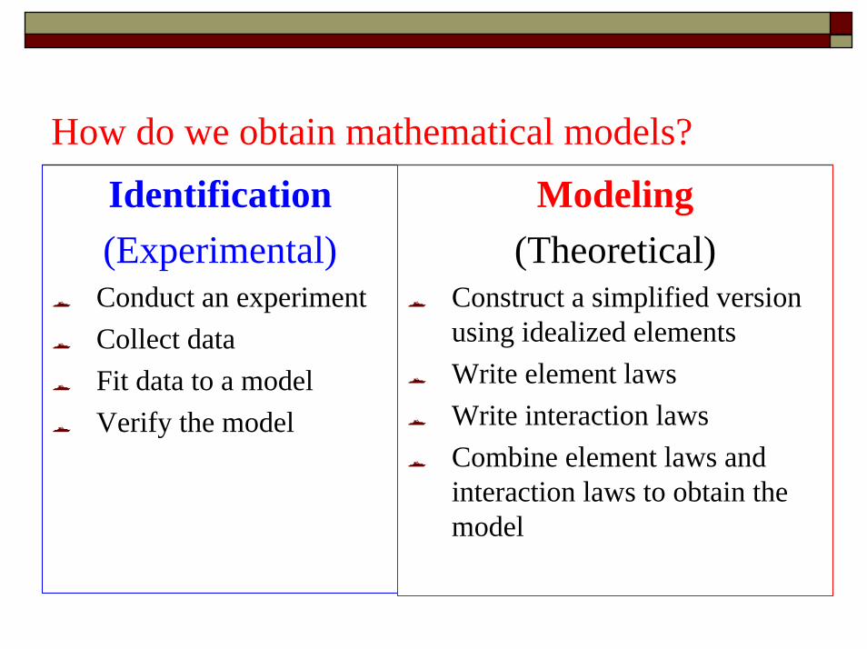
How do we obtain mathematical models?Modeling

(Theoretical)Construct a simplified version using idealized elementsWrite element lawsWrite interaction lawsCombine element laws and interaction laws to obtain the model

Identification(Experimental)Conduct an experimentCollect dataFit data to a modelVerify the model

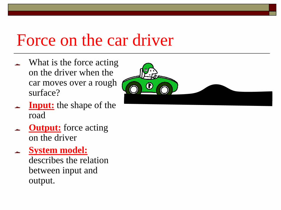
Force on the car driverWhat is the force acting on the driver when the car moves over a rough surface?Input: the shape of the roadOutput: force acting on the driverSystem model:describes the relation between input and output.

Modeling Using Idealized ElementsA simplified representation of the car by idealized elementsSelect relevant variablesWrite element lawsWrite interaction lawsObtain the model

Wheel axel

chassis

seat

driver

What is covered in this courseModeling of Systems

Idealized Elements (mechanical & electrical) Element lawsInteraction lawsObtaining the model

Solution of the ModelAnalytic solution using Laplace transform Simulation using SIMULINK

SummarySystems: set of components, achieve common objective

Inputs: signals affecting the systemOutputs: measured or calculated variables Process: relating input and output

Modeling: Derive mathematical description of system

Simulation: solving the mathematical model

Examples of modeling and simulationTopics covered in the course

SE 207: Modeling and SimulationUnit 1

Introduction to Modeling and Simulation

Lecture 2: Classification of systems

Reading Assignment: Chapter 1

Classification of SystemsSystems can be classified based on different criteria

Spatial characteristics: lumped & distributed Continuity of the time variable:continuous & discrete-time & hybridQuantization of dependent variable: Quantized & Non-quantized Parameter variation: time varying & fixed (time-invariant) Superposition principle: linear & nonlinear

Continuity of time variable

t tt0 t1 t2

Continuous-time SignalThe signal is defined for all t in an interval [ti, tf]

Discrete-time Signal

The signal is defined for a finite number of time points {t0, t1,…}

Give ExamplesGive examples of

continuous time signal

Discrete time signal

Examples of signals

t tt0 t1 t2

Temperature Sensor that provides Continuous reading of the temperature

temperature

Digital Temperature Sensor that provides reading of the temperature every 30 Seconds

Classification of Signals

Continuous-time,nonquantized

(Analog signal)Discrete-time,nonquantized

Continuous-time,quantized Discrete-time,quantized

(Digital Signal)

Classification of Signals and Systems

Classification of Signals

Classification of Systems

Classification of SystemsSystems are classified based on

• Spatial Characteristics (physical dimension,size)

• Continuity of time

• Linearity

• Time variation

• Quantization of variables

Spatial CharacteristicsLumped Models:Lumped models are obtained by ignoring the physical dimensions of the system.

• A mass is replaced by its center of mass (a point of zero radius)

• The temperature of a room is measured at a finite number of points.

• Lumped models can be described by a finite set of state variables.

Distributed Models:• Dimensions of the system is considered

• Can not be described by a finite set of state variables.

Spatial Characteristics

Lumped Models:• Only one independent variable ( t )

• No dependence on the spatial coordinates

• Modeled by ordinary differential equations

• Needs a finite number of state variables

Distributed Models:• More than one independent variable

• Depends on on the spatial coordinates or some of them.

• Modeled by partial differential equations

• Needs an infinite number of state variables

QuestionsGive examples of

Distributed modelsLumped models

Continuity of timeContinuous Systems:The input, the output and state variables are defined over a range of time.

Discrete Systems:The input, the output and state variables are defined for t={t0,t1,t2,….}. For other values of t, they are either undefined or they are of no interest.

Hybrid Systems:Contains both continuous-time and discrete time subsystems

Quantization of the Dependant VariableQuantized variable: The variable is restricted to a finite or countable number of distinct values

Non-Quantized variable: The variable can assume any value within a continuous range.

Classification of Signals

Continuous-time,nonquantized

(Analog signal)Discrete-time,nonquantized

Discrete-time,quantized

(Digital Signal)Continuous-time,quantized

QuestionsGive examples of

Continuous signalContinuous systemDiscrete signalDiscrete system

Parameter VariationsSystems can be classified based on the properties of their parameters

Time-Varying Systems

Characteristics changes with time. Some of the coefficients of the model change with time

Time-Invariant Systems

Characteristics do not change with time.

The coefficients are constants

LinearityA system is linear if it satisfies the super positionprinciple. A system satisfies the superposition principle if the following conditions are satisfied:

1. Multiplying the input by any constant, multiplies the output by the same constant.

2. The response to several inputs applied simultaneously is the sum of individual response to each input applied separately.

Linearity

)()(3)()(2)(

dt u(t) y(t)

2

2

0

tutytdt

tdytutty

=+

=

= ∫

u(t) y(t)

Examples of Linear Systems Examples of Nonlinear Systems

)()()()()(2)(

dt (t)u y(t)2

0

2

tutytudt

tdytutty

=+

=

= ∫

LinearityExample of linear systems

∫ ∫

∫∫

∫∫

∫∫

==⇒=

+=+=

+==

+=

==

2

0

2

0111

21

2

02

2

01

2

021

2

0

21

2

022

2

011

(t)dtu(t)dtuky(t)(t)uu(t)

(t)y(t)ydt (t)u(t)dtu

]dt (t)u(t)[udt u(t) y(t)

(t)u(t)uu(t)

dt (t)u (t)y,dt (t)u (t)y

kk

Both conditions

are satisfied

u(t) y(t)

LinearityExample of non-linear systems

(t)y(t)y general (t)y(t)ut2(t)ut2u(t)

u(t),(t)ut2 (t)y

11

111

1

11

−≠

==−=

−=

=

In

(t)u

If the input is multiplied by (-1) the output remains unchanged. This system is nonlinear

u(t) y(t)

Classification of SystemsSpatial characteristics lumped distributed

Continuity of the time variable

continuous discrete-time hybrid

Parameter variation Fixed (time-invariant)

time varying

Quantization of dependent variable

QuantizedNon-Quantized

Superposition principle linear nonlinear

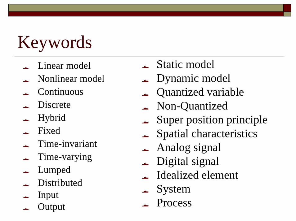
KeywordsStatic modelDynamic modelQuantized variableNon-QuantizedSuper position principleSpatial characteristicsAnalog signalDigital signalIdealized elementSystem

Linear modelNonlinear modelContinuousDiscreteHybridFixedTime-invariantTime-varyingLumpedDistributedInputOutput Process

SummaryClassification of signals

Continuous, discrete, quantized, non-quantizedClassification of Systems

Continuous-time systems, discrete-time systemsHybrid systemsLinear systems, nonlinear systemsTime-varying, time-invariant,