sections 7.3, 7.4, and 7 - university of south...

7.3 Further aspects of the t test7.4 Association vs. causation7.9 More on hypothesis tests

Sections 7.3, 7.4, and 7.9

Timothy Hanson

Department of Statistics, University of South Carolina

Stat 205: Elementary Statistics for the Biological and Life Sciences

1 / 23


Hypothesis tests and confidence intervals

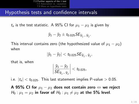
ts is the test statistic. A 95% CI for µ1 − µ2 is given by

y1 − y2 ± t0.025SEY1−Y2.

This interval contains zero (the hypothesized value of µ1 − µ2)when

|y1 − y2| < t0.025SEY1−Y2,

that is, when ∣∣∣∣ y1 − y2

SEY1−Y2

∣∣∣∣ < t0.025,

i.e. |ts | < t0.025. This last statement implies P-value > 0.05.

A 95% CI for µ1 − µ2 does not contain zero ⇔ we rejectH0 : µ1 = µ2 in favor of H0 : µ1 6= µ2 at the 5% level.

2 / 23


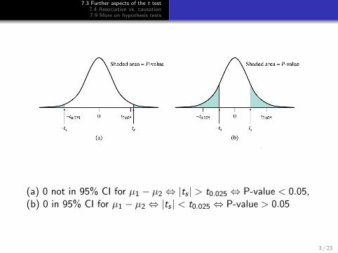
(a) 0 not in 95% CI for µ1 − µ2 ⇔ |ts | > t0.025 ⇔ P-value < 0.05,(b) 0 in 95% CI for µ1 − µ2 ⇔ |ts | < t0.025 ⇔ P-value > 0.05

3 / 23


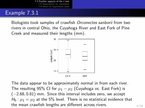
Example 7.3.1

Biologists took samples of crawfish Orconectes sanborii from tworivers in central Ohio, the Cuyahoga River and East Fork of PineCreek and measured their lengths (mm).

The data appear to be approximately normal in from each river.The resulting 95% CI for µ1 − µ2 (Cuyahoga vs. East Fork) is(−2.68, 0.81) mm. Since this interval includes zero, we acceptH0 : µ1 = µ2 at the 5% level. There is no statistical evidence thatthe mean crawfish lengths are different across rivers. 4 / 23


Interpretation of α

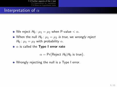
We reject H0 : µ1 = µ2 when P-value < α.

When the null H0 : µ1 = µ2 is true, we wrongly rejectH0 : µ1 = µ2 with probability α.

α is called the Type I error rate

α = Pr{Reject H0|H0 is true}.

Wrongly rejecting the null is a Type I error.

5 / 23


Type II error rate β

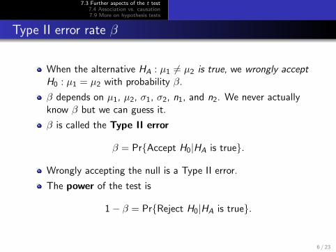
When the alternative HA : µ1 6= µ2 is true, we wrongly acceptH0 : µ1 = µ2 with probability β.

β depends on µ1, µ2, σ1, σ2, n1, and n2. We never actuallyknow β but we can guess it.

β is called the Type II error

β = Pr{Accept H0|HA is true}.

Wrongly accepting the null is a Type II error.

The power of the test is

1− β = Pr{Reject H0|HA is true}.

6 / 23


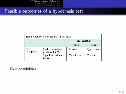
Possible outcomes of a hypothesis test

Four possibilities.

7 / 23


Example 7.3.3 Marijuana and the pituitary

Cannabinoids can be transmitted from the mother to fetus(through the placenta) and to the infant through milk. Onegroup of mice are given cannabinoids, the other group arecontrols. Say µ1 is mean pituitary function among cannabinoidmice and µ2 is mean pituitary function among controls.

We test H0 : µ1 = µ2 vs. HA : µ1 6= µ2.

If we make a Type I error, then we are (wrongly) sayingmarijuana affects the pituitary of offspring and there could beuneccessary widespread panic.

If we make a Type II error, then we are (wrongly) saying thatmarijuana use does not affect offspring pituitary function.Then marijuana-using mothers may choose to continuemarijuana use, and ultimately negatively affect their kid(s).

8 / 23


Experiments vs. observational studies

The response variable Y measures the outcome of interest,and

the explanatory variable X is used to explain or predict theoutcome. So far this has been “group,” e.g. treatment orcontrol.

In an experiment we can tease out whether changing Xaffects the distribution of Y (usually focus on mean). Thisimplies a causal relationship; changing X causes Y to change.

With observational studies we cannot discuss causality, butrather only association. That is we can find out whether Xand Y are related, but not whether X causes Y to change.

Whether we can discuss how X causes Y , or only how X isrelated to Y has to do with how the data were collected.

9 / 23


Example 7.4.1 hematocrit in males and females

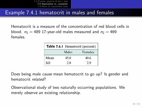
Hematocrit is a measure of the concentration of red blood cells inblood. n1 = 489 17-year-old males measured and n2 = 469females.

Does being male cause mean hematocrit to go up? Is gender andhematocrit related?

Observational study of two naturally occurring populations. Wemerely observe an existing relationship.

10 / 23


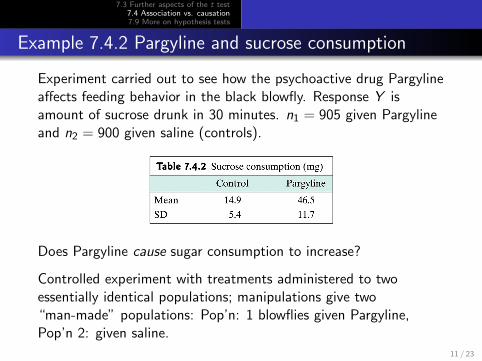
Example 7.4.2 Pargyline and sucrose consumption

Experiment carried out to see how the psychoactive drug Pargylineaffects feeding behavior in the black blowfly. Response Y isamount of sucrose drunk in 30 minutes. n1 = 905 given Pargylineand n2 = 900 given saline (controls).

Does Pargyline cause sugar consumption to increase?

Controlled experiment with treatments administered to twoessentially identical populations; manipulations give two“man-made” populations: Pop’n: 1 blowflies given Pargyline,Pop’n 2: given saline.

11 / 23


Experiment vs. observational study: cholesterol

Your book has a nice example illustrating the difference.

In a clinical trial, experiments randomly assign the samepopulation to a cholesterol-lowering drug or a control. At theend of the study n1 = 100 treatment and n2 = 100 controlshave their blood cholesterol measured and a two-sample t-testis conducted to determine if there’s a difference.

If there is a difference, we can infer that the drug causescholesterol to go down; that’s the only difference in thepopulations!

12 / 23



In an observational study, a random sample of people fromCamden, SC are measured for cholesterol; several othervariables are also recorded, including age, gender, weight,height, blood pressure, marriage status, etc.

It’s found that those under 30 have lower cholesterol thanthose over 50 years old using a two-sample t-test, fromsamples of size n1 = 453 and n2 = 229.

13 / 23



Can we conclude that the cholesterol increase is due to age?

Not necessarily; age might be directly related to cholesterol,but it might be that those over 50 ate more bacon and eggstheir whole life than those under 30, due to dietary changes inthe American diet over time.

Here, diet is said to be confounded with age. Diet is really thecausal factor, not age.

In other words: (a) diet is related to age, and (b) diet isrelated to cholesterol, so (c) cholesterol is related to age.

How would we determine whether age is related tocholesterol? Hint: we’d have to conduct a very expensiveexperiment over a long time...

14 / 23


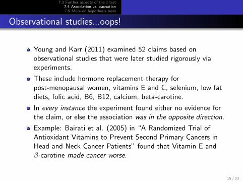
Observational studies...oops!

Young and Karr (2011) examined 52 claims based onobservational studies that were later studied rigorously viaexperiments.

These include hormone replacement therapy forpost-menopausal women, vitamins E and C, selenium, low fatdiets, folic acid, B6, B12, calcium, beta-carotine.

In every instance the experiment found either no evidence forthe claim, or else the association was in the opposite direction.

Example: Bairati et al. (2005) in “A Randomized Trial ofAntioxidant Vitamins to Prevent Second Primary Cancers inHead and Neck Cancer Patients” found that Vitamin E andβ-carotine made cancer worse.

15 / 23


From Bairati et al. (2005)

Although low dietary intakes of antioxidant vitamins and minerals have been associated

with higher risks of cancer, results of trials testing antioxidant supplementation for

cancer chemoprevention have been equivocal. We assessed whether supplementation

with antioxidant vitamins could reduce the incidence of second primary cancers among

patients with head and neck cancer. Methods: We conducted a multicenter,

double-blind, placebo-controlled, randomized chemoprevention trial among 540

patients with stage I or II head and neck cancer treated by radiation therapy between

October 1, 1994, and June 6, 2000. Supplementation with α-tocopherol (400 IU/day)

and β-carotene (30 mg/day) or placebo began on the first day of radiation therapy

and continued for 3 years after the end of radiation therapy.

16 / 23


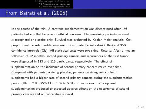
From Bairati et al. (2005)

In the course of the trial, β-carotene supplementation was discontinued after 156

patients had enrolled because of ethical concerns. The remaining patients received

α-tocopherol or placebo only. Survival was evaluated by Kaplan-Meier analysis. Cox

proportional hazards models were used to estimate hazard ratios (HRs) and 95%

confidence intervals (CIs). All statistical tests were two-sided. Results: After a median

follow-up of 52 months, second primary cancers and recurrences of the first tumor

were diagnosed in 113 and 119 participants, respectively. The effect of

supplementation on the incidence of second primary cancers varied over time.

Compared with patients receiving placebo, patients receiving α-tocopherol

supplements had a higher rate of second primary cancers during the supplementation

period (HR = 2.88, 95% CI = 1.56 to 5.31)...Conclusions: α-Tocopherol

supplementation produced unexpected adverse effects on the occurrence of second

primary cancers and on cancer-free survival.

17 / 23


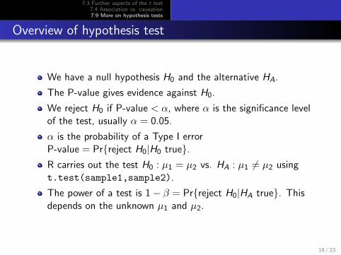
Overview of hypothesis test

We have a null hypothesis H0 and the alternative HA.

The P-value gives evidence against H0.

We reject H0 if P-value < α, where α is the significance levelof the test, usually α = 0.05.

α is the probability of a Type I errorP-value = Pr{reject H0|H0 true}.R carries out the test H0 : µ1 = µ2 vs. HA : µ1 6= µ2 usingt.test(sample1,sample2).

The power of a test is 1− β = Pr{reject H0|HA true}. Thisdepends on the unknown µ1 and µ2.

18 / 23


How to pick H0 and HA?

Since the P-value only gives evidence toward HA, HA is whatwe want to show. Also called the “research hypothesis.”

H0 is the “status quo” – what we want to disprove.

In an experiement, H0 will always be that there is no meandifference between treatment and control.

19 / 23


More on P-values (p. 279)

The P-value of the data is the probability (assuming H0 istrue) of getting a result as extreme as, or more extreme than,the result that was actually observed.

The P-value is the probability that, if H0 were true, a resultwould be obtained that would deviate from as much as (ormore than) the actual data do.

The P-value of the data is the probability (assuming H0 istrue) of getting a result as deviant as, or more deviant than,the result actually observed where deviance is measured asdiscrepancy from H0 in the direction of HA.

The P-value is not the probability that the null hypothesis istrue.

20 / 23


Review of important ideas so far

Test H0 : µ1 = µ2 vs. HA : µ1 6= µ2.

Test statistic is ts = (Y1 − Y2)/SEY1−Y2.

P-value Pr{|Tdf | > |ts |} is probability of seeing biggerdifference in sample means than actually saw, given H0 is true.

Small P-value gives evidence towards HA : µ1 6= µ2.

Reject H0 : µ1 = µ2 if P-value < α, usually α = 0.05.

α is called the significance level of the test, it is theprobability of a Type I error.

Type I error is rejecting H0 : µ1 = µ2 when H0 is really true.

Type II error is accepting H0 : µ1 = µ2 when HA : µ1 6= µ2 isreally true.

The power of the test is Pr{reject H0|HA true}.

21 / 23



A 95% confidence interval for µ1 − µ2 includes zero if andonly if we accept H0 : µ1 = µ2 vs. HA : µ1 6= µ2 at the 5%significance level.

The t-test needs normal data for small sample sizes, sayn1 < 30 or n2 < 30. Check this with a probability plot.

In large samples, we don’t worry about the normalityassumption.

In small samples, the permutation test in Section 7.1 alwaysgives the correct P-value, even when data are not normal.

22 / 23



Rejecting H0 : µ1 = µ2 means that the outcome is associatedwith group membership (e.g. treatment or control) inobservational studies.

In a carefully controlled experiment Rejecting H0 : µ1 = µ2

may confer a causal relationship.

“Association is not causation” necessarily.

A confounding variable is one that changes with groupmembership, but really causes the response to change.

In general a P-value is the probability of getting any teststatistic more “deviant” than what we saw in the direction ofHA, assuming H0 is true.

23 / 23

sections 7.3, 7.4, and 7 - university of south...

Documents