HAL Id: hal-03393065https://hal-sciencespo.archives-ouvertes.fr/hal-03393065

Preprint submitted on 21 Oct 2021

HAL is a multi-disciplinary open accessarchive for the deposit and dissemination of sci-entific research documents, whether they are pub-lished or not. The documents may come fromteaching and research institutions in France orabroad, or from public or private research centers.

L’archive ouverte pluridisciplinaire HAL, estdestinée au dépôt et à la diffusion de documentsscientifiques de niveau recherche, publiés ou non,émanant des établissements d’enseignement et derecherche français ou étrangers, des laboratoirespublics ou privés.

Distributed under a Creative Commons Attribution - NoDerivatives| 4.0 InternationalLicense

Social Responsibility and Firm’s ObjectivesMichele Fioretti

To cite this version:

Michele Fioretti. Social Responsibility and Firm’s Objectives. 2020. �hal-03393065�

Discussion Paper

SOCIAL RESPONSIBILITY AND FIRM’S OBJECTIVES

Michele Fioretti

SCIENCES PO ECONOMICS DISCUSSION PAPER

No. 2020-01

Social Responsibility and Firms’ Objectives*

Michele Fioretti†

February 3, 2020

Abstract

This paper shows that firms’ objectives can extend beyond profit maximization. Ifocus on a for-profit firm that offers charity auctions of celebrities’ belongings. Thefirm’s donations affect both revenues and costs. Counterfactuals from a structuralmodel comparing the actual donations with the profit-maximizing benchmark indicatethat the firm donates beyond profit-maximization. Linking this result to a changein the capital structure, I demonstrate that the firm’s objectives include both profitsand donations. I also estimate a modest increase in consumers’ willingness to paydue to donations, suggesting that demand cannot explain firms’ investments in socialresponsibility.

JEL classifications: L21, D64, C14Keywords: objectives of the firm, profit maximization, corporate social responsibility,donations, structural estimation, externalities

*I am indebted to Geert Ridder, Giorgio Coricelli and Roger Moon for their invaluable help and sugges-tions, as well as their continuous support and encouragement. I would also like to thank Ali Abboud, SusanAthey, Jorge Balat, Vittorio Bassi, Thomas Chaney, Khai X. Chiong, Kenneth Chuk, Jonathan Davis, DanielElfenbein, Cary Frydman, Aryal Gaurab, Giovanni Gardelli, Emeric Henry, Chad Kendall, Asim Khwaja,Tatiana Komarova, Rocco Macchiavello, Kristof Madarasz, Lorenzo Magnolfi, Benjamin Marx, FrancescaMolinari, Jia Nan, Hashem Pesaran, Jean-Marc Robin, Aloysius Siow, Matthew Shum, Jorge Tamayo, Gi-anluca Violante and Sha Yang. This paper also benefited greatly from the comments of the participants toseminars at Carlos III, CalState Long Beach, Caltech, Imperial College, Sciences Po, and Warwick and atthe 2019 ESSO, 2018 EEA-ESEM, the 2016 and 2018 IIOC, the 2017 EMCON, the 2016 IAAE and the 2016California Econometrics Conference, where previous versions of this paper were presented. I gratefullyacknowledge funding from USC INET and IAAE (IAAE Travel Grant). Computation for the work de-scribed in this paper was supported by the University of Southern California’s Center for High-PerformanceComputing (hpc.usc.edu). All errors and omissions are my own.

†Sciences Po, Department of Economics, 28 Rue des Saints-Peres, 75007, Paris, France. e-mail:michele.fioretti@sciencespo.fr

1 Introduction

The economic literature has gradually changed its vision of the consumer, who is nowincreasingly considered as having some type of social preferences such as altruism. Incontrast, the perception of the firm’s objective has seen very little evolution. The firm istypically modeled as maximizing profits. This assumption drives most of the standardresults on the functioning of markets, and it also allows researchers to recover costs orsupply curves (e.g., Olley and Pakes, 1996, De Loecker et al., 2016).

There are many reasons to believe that firms do not maximize profits. On the one hand,managerial costs (Ellison et al., 2016, DellaVigna and Gentzkow, 2019) and behavioral biases(Ellison, 2006, Hortacsu et al., 2019) can constrain a firm’s decisions. On the other hand,firms may not limit themselves to pursue market value, as, more broadly, shareholders’welfare often directs firms’ decisions as well (e.g., Hart and Zingales, 2017).

In this paper, I provide evidence that some firms are not simple profit maximizers. Istudy the strategic decisions of a for-profit firm, Charitystars, which offers online charityauctions of celebrities’ belongings.1 In each auction, the firm donates a fraction of thetransaction price to a charity. The fraction donated is decided by the firm and the providerof the item – mainly the charity itself, a connected celebrity or individual. Both the fractiondonated and the charity are known to consumers.

This environment offers several advantages to empirically identify the firm’s objectives.First, the fraction donated reflects how socially responsible the firm is in each auction. Thistype of social responsibility is directly measurable and salient to consumers. Second, costsare observed because the firm always sets its reserve price to cover the cost of procuringthe item, which depends on the donation. Therefore, this is an ideal setting to measurehow social responsibility impacts profits.

I find that Charitystars does not set its donation according to profit maximization.After building and structurally estimating a tailored model of demand and supply, I showthat Charitystars’s average donation (70% of the transaction price) is much larger thanthe profit-maximizing donation (25%). The firm could more than double its profits bybehaving optimally. After ruling out alternative potential explanations, I exploit a changein Charitystars’s capital structure to argue that the firm’s objectives are not limited toprofits, but extend to donating to charities.

Methodologically, Charitystars faces a tradeoff between (i) increasing the fractiondonated to stimulate demand by altruistic bidders and get better acquisition costs from

1With offices in London, Milan, and Los Angeles, Charitystars is a for-profit start-up with almost $4min equity. Since its foundation in 2013, the company generated over $10 million for charities and nonprofitorganizations. For more information, see www.charitystars.com.

1

donors, and (ii) decreasing the fraction donated to increase the profit from each auction.Without a structural model, I show evidence that this tradeoff exists. However, sincethe elasticities of demand and acquisition costs to donations are unobservable from dataalone, I build a structural model to evaluate the firm’s objectives quantitatively. The modelexploits variation in the fraction donated to estimate both how consumers’ willingness topay and procurement costs vary with social responsibility.

On the demand side, I model bidders’ utility as a function of their private values forthe item and their prosocial preferences (e.g., Goeree et al., 2005, Engers and McManus,2007). I envision consumers as impure altruistic bidders who derive utility both from theirdonations and from the donations of others (Andreoni, 1990). Theoretically, I show thatthe presence of altruistic consumers does not necessarily grant greater revenues to the firm.For instance, if bidders derive large utility from somebody else’s donations, transactionprices can decrease when the auctioneer donates more because high-value bidders shadetheir bids to let other bidders win the auction. To quantify how preferences impact prices,I show that cross-auction variation in the fraction donated nonparametrically identifies themodel under the restriction that a bidder’s consumption value for the item is independentof the fraction donated. I test and do no reject this restriction in the data.

The model fits the data well, with estimated expected revenues within 10% of the real-ized ones. Prices on Charitystars command only a small premium as bidders’ willingnessto pay increases with the fraction donated. At the same time, donations carry a high directcost in terms of foregone revenues: a counterfactual scenario where the firm does notdonate quantifies the loss in net revenues to be as large as e 260 per listing, or about 70%of the average transaction price. Thus, looking only at the demand side, the firm would bebetter off by running regular non-charity auctions.

Turning to the supply side, the firm purchases the item from providers (mainly charitiesand celebrities) previous a payment, and contracts on the fraction of the auction priceto be donated back to the charity. To estimate how the procurement cost varies with thefraction donated, I exploit a piece of information provided directly by advisors of thefirm: the firm sets the reserve price to break-even. I find that procurement costs decreasein the fraction donated, implying negative marginal costs, and explain this result with abargaining model. The estimation shows that the optimal donation is about 25% of thetransaction price, yet the average donation in the data is 70%, indicating that Charitystarsis far from a pure profit maximizer.

This finding points to donations as an additional objective of the firm. Using empiricaland anecdotal evidence, I rule out potential alternative explanations such as biased beliefson bidders’ willingness to pay, and reputation-building. Then, I exploit the entry of a

2

venture fund in Charitystars’s equity to corroborate my claim. Although the entry did notimply a change in management, the average donation dropped from 70% to 50% after theentry. Because the fund entered for a capital gain, it stirred the company towards betterprofitability, inducing a shift in objectives. To rationalize the large pre-entry donation,Charitystars’s objective function should weigh its profits 60% and its donations 40%.This finding is in line with recent results in the finance literature showing that sociallyresponsible actors invest in social impact firms despite being less profitable (Riedl andSmeets, 2017, Barber et al., 2019).

Relation to the Literature. Several related research papers support my conclusions onboth revenues and costs. On the revenue side, I estimate modest price elasticities of theorder seen in other papers studying bidder’s behavior in charity auctions (e.g., Elfenbeinet al., 2012). Given how salient are Charitystars’s donations for consumers, my findingssuggest that consumer demand cannot explain firms’ prosocial inclinations. In the samevein, looking across more than 400 US companies, Gartenberg et al. (2019) finds that afirm’s sales do not correlate with its social purpose. On the cost side, giving is profitablebecause it changes Charitystars’s cost-structure as its money-making ability and ethicalconcerns are not separable. Quoting Hart and Zingales (2017), if consumers and investorsvalue charitable donations, why “would they not want the companies they invest in todo the same?” Socially responsible shareholders may see this company as an opportunityto sustain their donations over time while even receiving dividends. Under this logic,Charitystars cares not only about its profitability but also about its total giving.

The evidence that social responsibility is conducive to higher economic or financialreturn is sparse. Although Eichholtz et al. (2010) find a substantial price premium forenergy-efficient buildings, a meta-analysis of over 160 papers finds only a small positivecorrelation between investments in corporate social responsibility (CSR) and profits, andsuggest that causation may well flow from profits to CSR (Margolis et al., 2007). A reasonfor these conflicting views lies in studying the relation between CSR and profits acrossfirms, rather than within a firm: not only the decision to adopt CSR may well dependon unobserved firm-specific factors (Benabou and Tirole, 2010), but also CSR activitiesare considerably heterogeneous, complicating comparison across firms (Chatterji et al.,2009, Kotsantonis and Serafeim, 2019). Moreover, this variation may interact in surprisingways, sometimes reducing a firm’s perceived social impact by, for example, disseminatingmisleading information of environmental friendliness (Lyon and Maxwell, 2011) and bygiving to charities to influence connected congress members (Bertrand et al., 2018).

My findings suggest that addressing whether CSR increases profits by comparingfirms’ outputs may lead to inconclusive results if firms choose suboptimal levels of social

3

responsibility. Rather than comparing across firms, I avoid these issues by studying howa firm’s social responsibility strategy departs from the profit-maximizing one. At thesame time, I test a causal link between profitability and social responsibility through thelenses of a theoretical model of a firm that sells to socially-oriented consumers (e.g., Baron,2001, Bagnoli and Watts, 2003, Besley and Ghatak, 2007). My findings strongly indicatethat consumers do not react substantially to socially responsible campaigns, even in anenvironment where social responsibility is especially salient. Therefore, demand concernsseem unlikely to stimulate firms to invest in CSR.

This paper is also related to a growing literature investigating firms’ conduct. Forexample, Duarte et al. (2020) find that Italian cooperatives behave in the same manneras their for-profit competitors. On the other hand, Macchiavello and Miquel-Florensa(2019) also show that coffee intermediaries pay Colombian coffee farmers more than whatimplied by profit maximization, but explain this finding through resale price maintenancepolicies rather than fair trade or social responsibility. Principal-agency problems betweenshareholders and management (e.g., Hart, 1995, Liljeblom et al., 2011) and managerialquality (e.g., Bloom and Van Reenen, 2007, Goldfarb and Xiao, 2011, Adhvaryu et al., 2018)are other classic reasons why firms fail to maximize profits.

Suboptimal choices are also observed in the National Football League as certain playscalled by coaches do not maximize the probability of victory (Romer, 2006), and teamsoften waste their top picks at the annual draft (Massey and Thaler, 2013). These papersspeculate that influence from shareholders and fans could sway decisions away fromoptimality. However, supporting empirical evidence using business data is lacking. Thispaper fills this gap by demonstrating that firms can be influenced by concerns that areexternal to profits.

2 Auctions on Charitystars

Charitystars is a for-profit internet company helping charities do fundraising, by offeringcharity auctions of celebrities’ memorabilia. Charitystars auctions a very broad spectrumof items, from VIP tickets to sport events to arts collectibles.2 Soccer is one of the mostpopular item categories with over 4,000 auctions held in 3 years. Moreover, Charitystars isa de facto monopolist in the market for actually worn soccer jerseys, on which I focus.3

2Charitystars is owned by its funding members, who also are managers in the company, and otherinvestors including funds.

3It is possible to find some worn soccer jerseys on eBay as well, but this marketplace is much thinnercompared to Charitystars. Moreover, as it will be shown in Section 6.3, bidders pay a charity premium onCharitystars, meaning that Charitystars bidders would lose money in case of resale.

4

Auction Format. On Charitystars, the auction winner wins the auctioned item and pays hisbid. The transaction price is then shared between Charitystars and a charity according to aknown sharing rule. The charity receiving the donation, as well as the fraction donated, areknown to all bidders before the auction. Donations are guaranteed by issuing certificates.

All Charitystars’s auctions involve a single item and employ an open, ascending-bidformat analogous to eBay. Bidders can also submit cutoff bids instead of a bid. Once acutoff is set, Charitystars will issue a bid equal to the smallest of the standing price andthe highest submitted cutoff price, plus the minimum increment. Importantly, the auctioncountdown is automatically extended by 4 minutes anytime a bid is placed in the last 4minutes of the auction. This effectively impedes sniping (Backus et al., 2017). After eachsold soccer jersey, if a fraction q of the transaction price is donated, the firm keeps 1− q ofthe price paid as net revenues.

All items are posted online on the firm’s website and advertised on the social media ofthe firm in a similar fashion. The listing webpage shows pictures of the item on the left ofthe screen. Bidders find a short description on the bottom of the page, together with theinformation on the recipient charity. A picture of a typical webpage at the time of the datacollection is in Appendix Figure D1.

Procurement. Charitystars procures the memorabilia mostly from footballers, teams, andcharities. The fraction donated is bargained between the firm and the provider of the item,who also requires a payment for procuring the item. Therefore, charities procuring the itemreceive both a fixed fee and a fraction donated. Charitystars’s minimum fee is 15% of thetransaction price, and increases if the provider requires a larger compensation to providethe item (see Appendix Figure D2). Importantly, talks with advisors and shareholders ofthe firm revealed that the firm sets the reserve price in soccer jersey auctions such that theportion of the reserve price that is kept by the firm equates procurement costs. Due to thecomplexity of setting the profit optimal reserve price, this simple scheme allows avoidinglosses.4

Data. I use publicly available data from Charitystars.com. The dataset is collected fromthe website and contains auctions of authentic soccer jerseys sold between July 1, 2015 andJune 12, 2017 (1,583 auctions). I focus on this period because it represents two consecutivefootball seasons. Figure 1 reports the number of auctions for each percentage donated. Allauctions where the fraction donated is higher than 85% are disregarded as they coincidewith special events. Throughout the paper, I let q denote the fraction donated.

For each auction, I observe all bids placed, the date and time of the bid, the bidder4The reserve price is not disclosed on the website. However, it is displayed in the HTML code of the

webpage. Whether bidders know the reserve price does not affect the analyses in the paper.

5

nationality, and the charity. I do not observe the auction start date, and I proxy the auctionlength as the days between the first bid posted and the closing day.5 I focus on listings ofsold items with at least two bidders, transaction prices in the range e 100 - e 1,000, andwith a minimum raise not larger than e 25 (1,109 auctions in total). The average minimumincrement is less than e 2.00, and the transaction price is greater than the reserve price inmore than 95% of the listings. On average (median) the winning bid is 2.9 (2) times largerthan the reserve price. All the variables are defined in detail in Appendix B and AppendixTable B1 display summary statistics for the main variables.

3 The Impact of Giving on Bidding: Empirical Evidence

The reduced form evidence in this section provides the foundation for modeling demandin later sections by illustrating how giving impacts prices and competition across bidders.

Intensive Margin. I first investigate whether greater transaction prices are associated withmore generous donations (q). To test this hypothesis, I run a set of regressions where thetransaction price is on the left-hand side and auction characteristics, including q, are onthe right-hand side. Table 1 displays results from the following OLS regressions

pricet = γ0 + xt γ + γqqt + εt, (3.1)

where t indexes the auctions. The vector of covariates, x, includes all variables other thanthe fraction donated, q. The columns of the table vary based on the definition of x, whichappears displayed in the bottom panel of the table. The jerseys are quite comparable acrossdifferent fraction donated as the latter variable is not correlated with the quality of theplayer wearing the auctioned jersey.6 The estimates indicate that a 0.1 increase in q, isassociated with a price increase between e 8.4 and e 9.4, or 2.9% of the average price. Thisresult points to a positive but small correlation between bids and donations.

Since the fraction donated is bargained between the provider of the item and Charitys-tars, γq could be inconsistent if unobserved characteristics of the item affect both bidders’valuations and the bargaining outcome (q). In this case, Table 1 could erroneously suggestthat bidders care for giving, while they only care for the unaccounted characteristics.

To account for endogeneity, I instrument a listing’s reserve price and q with the average

5The average length of Charitystars’s auctions is usually between 1 and 2 weeks.6To check whether jerseys worn by better players are associated with larger fraction donated, I down-

loaded player data from the FIFA videogames on the previous 5 years and checked the correlation betweenq and the overall player quality. The correlation is only between -0.07 and 0, excluding this channel. Thecorrelation between q and the other covariates is also small (lower than |0.25|).

6

q and the average reserve price across all concurrent auctions ending within ±5 days. Theinstruments are valid if the concurrent auctions are not correlated after controlling forcovariates. Identification would fail, for instance, if a charity procures several items for anadvantageous deal. This occurrence is accounted for by exploiting the connection betweena charity and a specific footballer or team. In particular, I control for the number of listingsof jerseys from the same team in the previous three weeks and for the same player in theprevious two weeks, as well as a charity counter. Hence, potential correlations acrossauctions are likely purged from the residual variation. Furthermore, I also control for theimportance of the match (e.g., a final), player quality, and charity characteristics.

Appendix Table C2 reports the OLS and the IV estimates. The instruments stronglypredict transaction prices, and the hypothesis of weak-instrument is rejected at 0.1% levelacross all columns. I include the average number of bidders across concurrent auctions(within 5 days) as an additional instrument for over-identification. The Sargan test doesnot reject the null hypothesis. The IV estimates are statistically significant and slightlylarger than the OLS ones, but less precise.

I also investigate whether the relation between the logarithm of prices and the fractiondonated is linear with a series of quantile regressions in Appendix Table C1.7 The nullhypothesis that the coefficients computed at different quartiles are the same to the OLSone is not rejected at common values (F test p-value 0.82), suggesting a small and linearrelationship between q and log prices.

In conclusion, bidders seem to react to donations. In particular, a 10% change in theaverage fraction donated results in about a 9.2% change in transaction prices. Relatedpapers found qualitatively comparable results. For example, Elfenbein and McManus(2010) estimated that prices in eBay charitable listings are, on average, 6% larger thancomparable non-charity ones, while within a controlled experiment Leszczyc and Rothkopf(2010) determined that a 40% donation leads to a 40% price increase.

Extensive Margin. Bidders do not seem to prefer more generous auctions. In the data, atotal number of 2,247 bidders compete on average in 5.34 different auctions. This averageincreases to 8.51 after excluding bidders who bid in only one auction. More than 80% ofthe bidders that place at least two bids, bid at least in two auctions with different fractionsdonated. The raw data show no correlation between the number of bidders joining anauction and q (Spearman correlation: 0.086).

I further investigate the impact of q on the extensive margin of giving with the following

7Appendix Figure D3 plots the coefficients.

7

Poisson regressions

log(E[number o f bidderst|xt,qt]) = γ0 + xt γ + γqqt + log(lengtht) + εt,

where t indexes the auctions. The variable length is the exposure variable and tells howmany days the auction lasted. Table 2 reports the estimated coefficients which should beinterpreted in terms of number of bidders per day. The results confirm the absence of acorrelation between q and the number of bidders. This conclusion is also reaffirmed wheninstrumenting q as previously done (Appendix Table C3).

Asymmetric Bidding. Before moving to the auction model, I show that the data fail toportray significant asymmetries in the way bidders bid within an auction. There are twomain asymmetries that can be inspected. First, as most jerseys belong to Italian teams (63%of the auctions) and most charities are Italian (90% of the auctions), bidders from differentnationalities could employ different bidding strategies. However, Appendix Table C6shows no effect of a winner’s nationality on prices. Second, some bidders can be collectorsof jerseys and may care less about donating. I define collectors as recurrent winners whowon more than the median number of auctions won (three). Table C7 in Appendix Cshows that recurrent winners do not pay more on average. Therefore, in the next sectionI study the behavior of symmetric bidders by modeling Charitystars’s auctions and inSections 5 and 6 I show how to identify and estimate the primitives of such model.

4 Demand Model: Altruism in Charity Auctions

A charity auction entails the donation of a portion of the transaction price to a charity. Ifbidders care for charitable giving, their utility should also include how much is earned bythe charity. In this section, I extend the seminal work on price-proportional auctions byEngelbrecht-Wiggans (1994) and Engers and McManus (2007) to fit the main characteristicof Charitystars’s online auctions, namely that only a fraction q < 1 of the final priceis donated. In this setting, I study both the optimal bidding strategy and the revenue-maximizing choice of q.

I model the additional utility from donating to a charity by β · q · price, where β

transforms the fund raised, q · price, in utils. Hence, β indicates the satisfaction fromwinning the auction and donating. Though losing bidders do not consume the item, and soreceive no consumption utility, they enjoy the fact that the charity gets funded. The rewardto the losing bidders is modeled by the term α · q · price. As charitable motives cannotexplain the full amount of one’s bid, the literature assumes that α, β ∈ [0,1). Therefore, the

8

realized utility to a bidder who values the private good v can be summarized by

u(v;α, β,q) =

v− b + β · q · price, if i wins,

α · q · price, otherwise.(4.1)

Despite its simplicity, the model implies different underlying rationale for giving depend-ing on the relative size of α and β. Appendix Table C8 summarizes the most commontheories of altruism.

The null hypothesis is that bidders are not interested in giving. If α = β = 0, the classictextbook equilibrium applies, and altruistic preferences in no way shape bidding. Biddersare purely altruistic when their utility does not depend on the identity of the donor, orwhen α = β > 0. In this case, they are solely moved by their compassionate concern for theactivities of the charity (Ottoni-Wilhelm et al., 2017).8

Selfish motives may also be present. For instance, bidders may take pride in donating(e.g., Andreoni, 1990, Fisher et al., 2008). In this case, β− α > 0 implies that bidders receivea “warm glow” when winning and donating. An extreme case is when bidders onlycare for their donations and have no intrinsic motivations (β > 0 but α = 0). This modelcaptures the role of social status or prestige in donation (e.g., Harbaugh, 1998).9

Leszczyc and Rothkopf (2010) provide empirical evidence for α > β > 0 using a fieldexperiment with manipulated charity auctions to assess overbidding. In such a “volunteershill” model, bidders derive more utility from others’ contributions than their own.

4.1 How Donations Impact Bids and Revenues

To find the optimal fraction donated for the auctioneer, knowledge of how demand varieswith q is necessary. Thus, I start by examining a bidder’s optimal bidding strategy as afunction of q. The following standard regularity assumption is maintained throughout.

Assumption 1. Regularity:

1. All n > 1 bidders have private and independent values for the auctioned item. Values aredrawn from a continuous distribution F(·) with density f (·) on a compact support [v,v];

2. The hazard rate of F(·) is increasing.

8A theoretical treatment of these auctions first appeared in Engelbrecht-Wiggans (1994), who analyzedauctions with price-proportional benefits to bidders (all bidders receive an equal share of the final price).

9β > 0, α = 0 is consistent with bidders receiving subsidies as is common in timber auctions (Athey et al.,2013).

9

The independent private value assumption is relaxed in the estimation by the inclusionof auction heterogeneity, which effectively allows for affiliated values. An alternativewould have all bidders valuing the jersey equally, but enjoying only imperfect signals ofthis value before bidding. Under such a common values scenario, the winner’s courseincreases in the number of bidders. As a result, bidders will shade their bids the morebidders join the auction. However, this prediction is refuted by the positive and significantcoefficients of the number of bidders in Table 1. Condition 2. of Assumption 1 ensures theexistence of a unique global optimum of the bidding function and it is important for theidentification of the primitives of the model {F(v),α, β}.

Optimal Bid. Due to the strategic equivalence between ascending and second-price charityauctions (Engers and McManus, 2007), the expected utility to a bidder with value v in asecond-price charity auction is

E[u(v;α, β,q)] = E[v− (1− q · β) · price, i wins

]︸ ︷︷ ︸i wins and pays price

+q · α · price · Pr(i’s bid is 2nd highest

)︸ ︷︷ ︸i loses and bids bi = price

+ q · α ·E[price, i’s bid is < 2nd highest

]︸ ︷︷ ︸i loses and price > bi

,

where, price denotes the second-highest bid as this is the price at which the second-highestbidder drops out of the auction. The expected utility is taken over three mutually exclusiveevents. In the first brackets the bidder wins the contest, pays the price, enjoys v andadditional utility from giving to the charity (β · q · price). In the second and third brackets,the bidder either drops out as a second-highest bidder or earlier. In either case, the bidderbenefits in proportion to the expected donation (α · q· expected price).

Focusing on the symmetric Bayesian Nash equilibrium of the second-price auctiongame, the equilibrium bid for a bidder with private valuation v and charitable parametersα and β in a symmetric second-price charity auction where the auctioneer donates q is

b∗(v;α, β,q) =

1

1+q·(α−β)

{v +

∫ vv

(1−F(x)1−F(v)

) 1−q·βq·α +1

dx

}, if α > 0 and q > 0,

v1−q·β , if α = 0 or q = 0.

(4.2)

This bid function is also optimal in ascending online auctions: in equilibrium a bidderwith value v drops out of the auction when price ≥ b(v;α, β,q). Although there is nodiscontinuity as α goes to 0, the second line of equation 4.2 implies that truthful biddingis optimal when q = 0 or α = 0 as in second-price auction with non-charitable bidders.

10

Therefore, this model includes the classic textbook second-price auction model.

Comparative Statics on q. Does greater fraction donated necessarily increase bids? Fromequation 4.2 this is true if α = 0. In this case, a marginal increase in q is equivalent to amarginal increase in β, implying greater satisfaction from winning the auction, leadingto greater bids. More generally, whether bids increase or decrease with q depends on themodel of giving, as shown in the following lemma.

Lemma 1. Bids are- increasing in q if β ≥ α;- decreasing in q in the interval (v,v], where v ∈ [v,v], if α > β.

Proof. See Appendix A.2.Under warm glow (β ≥ α) all bidders revise up their bids if q increases. The solid line

in Figure 2a depicts this case. The dotted and dashed lines instead refer to the derivativeof bids w.r.t. q for the voluntary shill model (β < α): bids increase for bidders with lowvalues, and increase for bidders with high values.

Due to the monotonic bidding strategies, bidders with high values are possible winnersof the auction. A marginal change in q has two effects if α is large enough. First, it intensifiesthe degree of substitution between winning the auction and gaining from somebody else’scontribution to the charity (Benabou and Tirole, 2006). The substitution effect is moresignificant for high-value bidders, and so they are the ones to revise their bids down.

Second, low-value bidders affect their payoff only when they rank as the second-highestbidder. Thus, as their bid is complementary to that of a bidder with higher valuation, theyraise their bid in the hope of extracting more surplus from the winner. A comparison of thedotted and dashed lines in Figure 2a supports this idea: more low-value bidders increasetheir bids when they believe they are more likely to rank high in the auction. This beliefincreases with the variance of the distribution of private values (dotted line).

Therefore, in a charity auction, optimal bids must balance not only the intensive margin(a bidder’s surplus) with the extensive margin (the probability of winning) but also anadditional margin representing free-riding.

Net Revenues and q. If the cost of procuring the item is sunk, a profit-maximizer auction-eer should set the fraction donated to maximize net revenues, or (1− q) times price.

The revenue-optimal fraction donated qR depends on the demand parameters{F(v),α, β}. In particular, when α = 0, increasing q does not increase net revenues tothe auctioneer, because the term q · β · price act as a discount factor. Net revenues are lowerthan non-charity auction revenues, and the auctioneer should not donate.

Charity auctions are more appealing to the auctioneer in case of cross-bidders external-

11

ities (α > 0).10 However, α should be small enough to prevent high-value bidders fromexcessively shading their bids. The next proposition determines the fraction donated, qR,that maximizes net revenues.

Proposition 1. Define η(pe,q) = ∂pe

∂qqpe as the elasticity of the expected price, pe, to the donation,

q. When α = 0, the auctioneer should not donate. When α > 0, the revenue maximizing donationsolves η(pe(qR),qR) =

qR1−qR

.

Proof. See Appendix A.3.Intuitively, net revenues first increase as the auctioneer increases q, reach a maximum,

before decreasing to zero for q = 1, in which case the auctioneer donates all he or shemakes. Net revenues have an inverted-U shape, which is maximized at qR. The ratioq/(1− q) is the ratio of what is donated to what is kept and is convex in q. The firm willincrease its donation rate until the marginal benefit from higher bids ((1− q)η) equatesthe marginal cost from donating an extra euro (q). This is evident from Figure 2b, wherenet revenues (right axis) are optimized at the q that sets η = q/(1− q).

The Role of Externalities. The previous theoretical exercises should be read in light of thelack of agreement in the empirical literature assessing the effect of donations on pricesand revenues in charity auctions. For instance, Leszczyc and Rothkopf (2010) attributedthe widespread overbidding in their experimental charity over non-charity auctions tosignificant externalities. However, their conclusion that α > β implies higher revenuesis only partially correct as it also requires enough incentives for low-value bidders toplace high bids, as shown in Figure 2a. This seems to be the case in their data as theirauctions averaged less than four bidders, and so low-value bidders havre high chances toset the price. In contrast, another field experiment with more than 15 potential biddersin each auction found charitable prices to sink below non-charity ones at a school charityauction (Carpenter et al., 2008). Given Proposition 1, this can be explained in terms of highexternalities as parents (bidders) may care more for the fundraising of the school than theirdonations.

Because of the central role played by the different models of giving in determiningauction outcomes, the next section shows how to identify both the consumption, F(v), andaltruistic preferences, α and β.

10The result on the auctioneer’s surplus mimics how donations impact bidders’ surplus. When α = 0, theexpected bidders’ surplus in a charity and non-charity auctions are the same. Thus the auctioneer cannotextract additional rents from holding a charity auction. Instead, bidders’ surplus is greater in charity auctionsif α > 0.

12

5 Nonparametric Identification of Demand

The identification of the primitives of the model, {F(v),α, β} is necessary to assess Char-itystars’s objectives. Take the following example: two identical auctions with differentfractions donated are observed. A mere comparison of prices across auctions could lead toincorrect conclusions on bidders’ preferences. For instance, if the prices in the two auctionsare close despite one auction is much more generous than the other, we may infer thatbidders are not altruistic. Instead, high-value bidders could be shading their bids in theauction with the higher fraction donated due to significant externalities (Proposition 1). Asa result, wrongly concluding that consumers are not altruistic has obvious repercussionson the optimal strategy of the auctioneer.

In this section, I first show identification in second-price charity auctions and thenextend the analysis to Charitystars’s auctions.

Second-Price Auctions. Identification relies on variation in the fraction donated (q) acrossotherwise identical auctions to exploit the information in the first-order conditions ofoptimal bidding and the monotonicity of the bid function. In what follows, denotethe observed distribution of bids by G(b(v;α, β,q);q), and the related inverse hazardrate by λG(b(v;α, β,q);q).11 Since the bids are invertible functions of private values, thedistribution of bids is equal to the distribution of private values.12 I use the last equivalenceto write the FOC of a bidder with value v bidding b(v;α, β,q) as

v = (1− β · q) · b(v;α, β,q) + α · q ·(

b(v;α, β,q)− λG(b(v;α, β,q);q))

. (5.1)

The equation shows that the private value must balance one’s bid plus the surplus thatcan be extracted if somebody else wins with a larger bid.

The unknowns are v on the left-hand side and α and β on the right-hand side. DespiteF(v) is identified directly from the empirical distribution of bids (G(b)), one can plugdifferent combinations of {α, β} in equation 5.1 and obtain the same F(v). A similar non-identification result holds in the estimation of risk aversion in first-price auctions. There,identification relies on either parametric quantile restrictions or variation in the numberof bidders across auctions (e.g., Lu and Perrigne, 2008, Guerre et al., 2009, Campo et al.,2011). However, these restrictions are of no use for nonparametric identification in English

11The inverse hazard rate of the bid distribution is λG(b(v;α, β,q);q) = 1−G(b(v;α,β,q);q)g(b(v;α,β,q);q) , while the inverse

hazard rate of the distribution of private values is λF(v) =1−F(v)

f (v) .12Under Assumption 1 the following relations hold: G(B) = Pr(b(v) < B) ≡ Pr(v < b−1(B)) = F(b−1(B)).

Therefore, G(b(v;α, β,q);q) = F(v). It follows that g(b(v))b′(v) = f (v).

13

charity auctions as, for instance, the number of bidders does not even appear in the FOCs.Inspecting equation 5.1, the right-hand side is strictly increasing and differentiable in

b(v;α, β,q), implying that no two different combinations of α and β yield the same vector ofpseudo-private values v.13 This remark ensures that every distribution F(.|α, β,q) (one foreach α, β combination given q) is unique by Theorem 1 in Guerre et al. (2000).14 Therefore,if two sets of auctions, A and B, with different fraction donated, qA , qB, are observed,the distribution of private values computed on each set of auctions using equation 5.1must be the the same at the true parameters {α0, β0}. Thus, {α, β} are nonparametricallyidentified by F(·;α0, β0,qA) = F(·;α0, β0,qB). Once α and β are identified, F(v) is identifiedfrom equation 5.1.

However, this strategy fails if a bidder’s consumption value, v, depends on q – e.g., ifhigh valued bidders systematically join auctions with greater fractions donated. Thus, thefollowing assumption is necessary for identification:

Assumption 2. Identification: F(·) does not depend on q.

The theoretical model in Section 4 automatically satisfies this assumption because itdefines F(v) as the unconditional distribution of private values. Section 3 also finds thatCharitystars’s bidders join multiple auctions without regard for q. Also, the same sectionshows no correlation between the number of bidders, other auction characteristics, and q.Finally, I formally test (and do not reject) the validity of Assumption 2 in Section 6.2.

Charitystars’s Auctions. To extend the previous result to Charitystars’ auction, it is im-portant to consider that not all bidders bid according to equation 4.2 in online auctions.First, the equivalence between English auctions and button auctions does not hold forthose bidders who place a low bid once, and then forget to update their bids. Second, inequilibrium, the winner pays a small increment over the price at which the second-highestbidder quits bidding, suggesting that not even the winning bidder bids according toequation 4.2.15 Therefore, G(b;q) , F(v) in online auctions, so that the unknown F(v) inequation 5.1 cannot be replaced with the emprical G(b;q) to solve the problem as in thesecond-price auction case.

However, the winning bid is the price at which the second-highest bidder drops out,and thus, the second-highest bidder solves 5.1 at this price. As a result, the distributionof the winning bid, Gw(b;q) , is equal to the distribution of the second-highest bid, which

13The term in parentheses of equation 5.1 is increasing in b if f ′(v) > − f (v)2

1−F(v) + g(b; ·)b′′(v; ·), which isalways true because of Assumption 1. This is also confirmed in the data.

14Theorem 1 in Guerre et al. (2000) relies on the same regularity conditions in Assumption 1.15The minimum increment across Charitystars auctions is e 1 for most auctions.

14

is a known function of the number of bidders and it is invertible in F(v). Therefore, thecounterfactual G(b;q) for a parallel second-price auction is directly identified from theempirical distribution of the winning bids and the number of bidders, which, in turn,allows the identification of α and β as in the second-price auction case above.

Proposition 2. Under Assumptions 1 and 2, {F(v),α, β} are nonparametrically identified byobserving two identical auctions with different fractions donated.

Proof. See Appendix A.4.Proposition 2 can also be extended to include a finite number of auction types (e.g.,

q ∈ {q1,q2, ...,qK}), as shown in Corollary 1 in Appendix A.5. The proof uses the panelstructure of the data to create a projection matrix that cancels out the left-hand side ofequation 5.1 to identify α and β as in Proposition 2.

6 Estimation of the Demand Model

In this section, I first lay out the estimation routine, which closely follows the identificationin Proposition 2. Section 6.2 reports the results and fit of the model, and Section 6.3quantifies the charity premium.

6.1 Structural Estimation

Following the main identification result, the primitives of the model {F(v),α, β} are esti-mated comparing two auctions with different fraction donated, q. Clearly, identificationfails if the two fractions donated are dangerously close to each other as the necessary rankcondition would not hold.16 According to Figure 1, the most frequent fraction donated inCharitystars’s data are 10%, 78% and 85%. Thus, estimation is performed on a sample ofauctions with q ∈ {10%,85%}.

Estimation is performed in three steps. The first step accounts for auction heterogeneity.In the second step, I determine the distribution of bids and construct the FOCs. Theprimitives are estimated in the third step of the routine.

First Step. I account for auction heterogeneity through a flexible regression of the log oftransaction prices on auctions, item and charity characteristics according to the following

16Appendix Table F1 reports Monte Carlo simulations showing that the estimated {α, β} are not consistentif qA is too close to qB.

15

regression of the transaction price on covariates

log(pricet) = γ0 + xt γ + bw,t, (6.1)

where t indexes the auctions and x includes all the variables in column 1 in Table 1,excluding q. The residual, bw,t, are interpreted as pseudo-winning bids from homogeneousauctions (e.g., Haile et al., 2003), and are a function of α, β, q and winners’ private values.

Appendix Table C9 reports the estimates from equation 6.1. These estimates controlsfor both observed and unobserved heterogeneity. In particular, the number of bids placed(given the number of bidders and the length of the auction) tells the level of competitionacross bidders within an auction that is not explained by x. If the auction is more appealingfor some unobservable characteristics, bidders are likely to control the auctions moreclosely than predicted by x. The increased supervision will result in more bids by the samebidders, and as a result, will account for unobserved quality.

Second Step. The distribution and density of bids are necessary to write equation 5.1.Following the identification, I first group bw,t based on q (either 10% or 85%) and determinethe distribution of bids, Gq(b), from the empirical distribution of the winning bid, Gq

w(b),for each group. The densities gq(b) are computed analogously.17 To compute the empiricalCDF and pdf of bw,t, I use a Gaussian kernel with bandwidths as in Li et al. (2002).18

Third Step. I build the two sets of FOCs as in equation 5.1 based on q. I match eachFOC for the auctions with q = 10% with a FOC of the auctions with q = 85% along thequantiles of the distributions of bids, i.e. FOCs with bids b10% and b85% are matched ifG(b10%;q = 10%) = G(b85%;q = 85%). In this way the left-hand side, vq, for each FOC isequal to its matched counterpart at the true {α0, β0}, implying that at each τ quantile ofthe distribution of values v10%

τ (α0, β0)− v85%τ (α0, β0) = 0. Thus, the criterion function is

min{α,β}

1T

T

∑τ

(v10%

τ (α, β) − v85%τ (α, β)

)2, (6.2)

where T is the number of auctions with q = 10%, under the constraint that {α, β} are in[0,1]. The distribution of private values F(v) is found as the empirical distribution of the

17The distribution of bids Gq(b) is the solution to Gqw(b) = nGq(b)n−1 − (n− 1)Gq(b)n, while its density

gq(b) solves gqw(b) = n(n− 1)Gq(b)n−2[1− Gq(b)]gq(b), where gq

w(b) is the empirical pdf computed on bw,t.18The bandwidth of the kernel estimators are hq

g = cq · T−1/5q for pdfs and hq

G = ca · T−1/4q for CDFs.

cq = 1.06 ·min{σa, IQRa/1.349}, Tq is the number of auctions, σq is the standard deviation and IQRq is theinterquantile range of bq

w,t for auctions with fraction donated q. I trim the data to deal with bias at the extremeof bw,t supports.

16

left-hand side of equation 5.1, after plugging in the estimated {α, β}.19

6.2 Estimation Results

Table 3 reports the results of the estimation. The identification requires a constant numberof potential bidders to perform the inversion in the second step. To avoid outliers, I setthe potential number of bidders at the 99th-quantile of the distribution of bidders (firstrow of the table), and report estimates for various values of n. The 95% confidence intervalare also reported in square brackets and are obtained by bootstrap. The estimates hardlyvary with the number of potential bidders and are always significant. Consistent withother studies (e.g., DellaVigna et al., 2012, Huck et al., 2015), the results provide evidencefor warm glow agents as β > α > 0 (see Section 4). Next, I provide evidence that the modelfits the data well.

Expected Revenues. I first examine simulated prices. To recover the expected price in anauction with n bidders, I plug the estimated primitives {F(v),α, β} in the bid equation 4.2and integrate it with respect to the density of the second-highest bid. In all the followinganalyses, I compute values in euros by summing back the median values of the covariatesin equation 6.1 (xt γ) to the expected price and exponentiating it.20

The differences between the observed prices across auctions with q = 10% and q = 85%are not statistically different from the expected average prices at the median number ofbidders. In particular, the model predicts the expected price to be e 388.73 when q = 85%while the average observed price when q = 85% and n = 7 is e 375.50, a 3.5% deviation(p-value: 0.613). Similarly, the model predicted expected price when q = 10% and n = 7is e 353.87, whereas the average price in the data is e 327.44, a 8.1% deviation (p-value:0.516). The model also adequately predicts prices for other numbers of bidders as shownin Appendix Figure D5, where I vary the number of bidders between 5 and 10, whichcorresponds to the interquartile range of the number of bidders.

Test to Identification. The estimation procedure relies on Assumption 2, which statesthat F(v) does not depend on q. A direct test to this assumption is to apply the esti-mated coefficients in the first step and the estimated α and β to a set of auctions withq < {10%,85%}. The identification strategy fails if the implied distribution of values differsfrom the estimated F(v).

19Appendix F performs a number of MonteCarlo simulations suggesting that the estimator is consistentand asymptotically normal.

20I exclude the number of bidders from x because it is already accounted for in the computation of thewinning bid.

17

I apply this procedure to the auctions with q = 78%. Figure 3 compares this counterfac-tual density of private values (dotted line) with the estimated densities from the auctionsat 10% (solid line). The two pdfs have similar shapes and the Kolmogorov-Smirnov testdoes not reject the null hypothesis of equality at 0.187 level. This test is rather conservativebecause the auction heterogeneity could impact prices when q = 78% differently comparedto the case when q ∈ {10%,85%}.

Over-Identification Test. To investigate whether bidders have different altruistic param-eters, I perform a simple over-identification test in Appendix Figure D6a. I group themoments in equation 6.2 based on whether they refer to quantiles above or below themedian, and estimate α and β for each sample. The plot compares the densities impliedby the two sets of altruistic parameters. The null hypothesis that the two pdfs are thesame cannot be rejected, meaning that the assumption of equal α and β in the poulation ofbidders is not rejected by the data.

Collectors. Appendix Figure D4 shows that the pseudo-winning bid of collectors (asdefined in Section 2) from equation 6.1 is not statistically different from that of non-collectors, further corroborating the assumption of symmetric bidding with respect to thedistribution of private values.

Instrumental Variables. As in Section 3, I correct for potential endogeneity in the reserveprice using instrumental variables. In particular, following the discussion in Section3, I instrument a listing’s reserve price with the average reserve price and the averagenumber of bids placed across all the other auctions ending within five days of the auction.Appendix Table C10 shows little change both in the estimated α and β. The F-test is 33.269,and the over-identification test statistics (Sargan test) has a p-value of 0.192.

Linearity of Bids. Section 2 shows a linear relation between log prices and fractionsdonated. Appendix Figure D6b replicates this result by plotting the simulated log bids (yaxis) for different fraction donated (x axis) (cf. Appendix Table C1 and Figure D3). I donot reject the linearity of the bid curves with respect to q via ANOVA, indicating that themodel adequately reproduces the descriptive results described in Section 3.

6.3 Is There a Charity Premium?

The existence of a charity premium is debated in the literature on charity-linked goodsas, for instance, some online sellers with low reputations donate to charities to look morereputable (Elfenbein et al., 2012). I leverage on the structural model to cleanly estimate thecharity premium and extend the counterfactual analysis to address whether donations

18

increase cashflows to Charitystars.

Charity Premium. Appendix Figure D7 shows that the distribution of bids (dotted line)stochastically dominates that of private values (solid line). Therefore, the expected transac-tion price is larger than the second-highest private value. The charity markup (dashed line,right axis) appears in Figure 4a as the percentage difference between the second-highestbid in charity auctions (solid line) over the second-highest private value (dotted line) fordifferent fraction donated. Although the markup increases with q it is capped at 15%. Thisvalue is close to the estimates in Elfenbein and McManus (2010) of a 12% premium whenthe auctioneer donates 100% from eBay’s Giving Works data. On the other hand, althoughElfenbein et al. (2012) find that eBay bidders leave a 6% markup for a 10% donation, I findalmost no charity premium when the auctioneer donates little. Therefore, Charitystars’sdemand is inelastic despite consumers’ willingness to pay increases in q.

Revenue Maximizing q. Figure 4b confirms that the estimated elasticity of demand tothe fraction donated (solid line) is extremely rigid. Proposition 1 states that the revenue-maximizing fraction donated is found at the intersection of the elasticity curve and theq/(1− q) curve (dotted line). The two curves intersect at q = 0: net revenues are beyonde 300 when the firm does not donate, and constantly decrease as q grows (dashed line,right axis). Charitystars can increase its net revenues by as much as e 250 on average byholding standard auctions.

Discussion. Despite the charity premium, the price increase does not compensate forthe amount donated. Although I look exclusively at soccer jerseys, the results could berelevant for charity-linked products more broadly because of the salience and ease ofmeasurement of Charitystars’s social responsibility. Consider the case of Product Red,a charity fighting HIV in Africa whose fundraising comes from partnering with largecorporations – e.g., Apple – which donate a portion of their revenues for specific goods.For instance, Montblanc Product Red trolleys currently sell for $865, of which $5 go toProduct Red. The fact that donations are generally smaller than 10% of the price on thiswebsite shows that consumers’ willingness to pay does not react substantially to firms’donations also in other markets.21

Consumers also face different incentives in an auction compared to the posted price en-vironment from the example above, where anyone can buy and donate. Gneezy et al. (2010)investigate the willingness to pay for a photograph right after riding a roller coaster–like

21Similarly, Tom Shoes, a shoe company which used to donate a pair of shoes for each pair sold, has recentlyreverted to a much more flexible $1 donation for every $3 it makes as the old one-for-one donation scheme wastoo expensive. Source: https://media01.toms.com/static/www/images/landingpages/TOMS_Impact/

TOMS_2019_Global_Impact_Report.pdf, page 69.

19

attraction in a US amusement park. The authors compare two strategies: posted price andpay-as-you-want plus a 50% donation. Their findings confirm my results: profits-per-ridenet of donations are non-statistically different between treatment and control groups.

In conclusion, the analysis suggests that demand is unlikely to drive firms’ prosocialinvestments. To address why Charitystars donates, the next section explores how donationsimpact marginal costs and profits.

7 Procurement Costs and the Profit Optimal Donation

Charitystars may find it profitable to donate if procurement costs are decreasing in thefraction donated. In this section, I first report empirical evidence of bargaining betweenCharitystars and the providers (mainly celebrities and charities). Conversations withadvisors of the firm also confirmed this. Leveraging on this knowledge, I then turn to thecost of procuring the item and the profit-optimal donation.

Evidence of Bargainig. I first provide empirical evidence of bargaining. I exploit a periodof the year where the relevant bargaining power is tilted toward the providers. The leadingEuropean soccer leagues are off in the inactive summer months of July and August, and,as objects become scarce, item providers should be more powerful. The data indicatethat the average fraction donated in the summer months is significantly larger than in theremaining months (Welch tests: qAugust = 0.775, qother = 0.698, with a one-sided p-value= 0.030, and qJuly&August,= 0.770 qother = 0.693, with a one-sided p-value < 0.001). Tocontrol for other variables, I run the following OLS regressions

qt = γ0 + xt γ + γm summer montht + εt, (7.1)

where summer month refers to either August or to both July and August. Table 4 reportsthe results, confirming the presence of bargaining between parties, as Charitystars is moregenerous when it has less bargaining power. The results are robust to the inclusion of morecovariates (even columns).

However, Charitystars could donate more to stimulate more bidders to join the auctionin these summer months, where the soccer leagues are inactive (though Table 2 suggests anull effect of changes in q on the extensive margin). To solve this potential endogeneityconcern, I use a similar instrumental variable approach to that in Section 2. I instrumentthe reserve price and the number of bidders with the mean of these variables for auctionshappening within five days of each auctions. Appendix Table C4 shows that the coefficients

20

of the IV regressions are very similar to the OLS regressions. The F-statistic indicates asufficiently strong first-stage (though the F-statistic is slightly below 10 in column 4), andthe hypothesis of weak IV is rejected in all columns. I also perform the Sargan test of over-identification by including the average number of displayed pictures across concurrentauctions and do not reject the null.

Estimation of Procurement Costs. Let us turn to the optimal decision of a profit-maximizing charitable auctioneers, who must select the fraction donated to maximizeprofits, knowing that costs vary with how much is donated. Given knowledge of thenumber of bidders, α, β and F(v), the problem of the auctioneer is

q∗ = arg maxq∈[0,1]

∫v(1− q)b(v,α, β,q)dF(2)

(n)(v)− c(q),

where F(2)(n)(v) is the distribution of the second highest private value out of the n bidders.

Denoting the expected price by pe and its elasticity to the donation by η, it yields

c′(q) =1− q

qηpe − pe. (7.2)

The optimal donation equates a change in costs due to a marginal increase in q with therelative change in net revenues. In Appendix A.6, I extend the monopolist problem aboveto allow for bargaining over the fraction donated between the firm and the provider ofthe item within the framework of Nash bargaining. The model’s first-order conditions canbe rewritten to yields an equation similar to equation 7.2 showing that, under the mildcondition that the net expected price is larger than the costs to the auctioneer, costs arestrictly decreasing in q. Comparing the net revenue-maximizing donation from Proposition1, qR, and the profit optimal donation, q∗, implies that q∗ > qR if c′(q) < 0. From Figure 4b,qR = 0, and if also c′(·) < 0, Charitystars optimal choice is to set q∗ > 0. This derivationshows the importance of the cost channel on the profitability of social responsibilityprograms (Hart and Zingales, 2017).

To avoid losses, Charitystars ensures that the smallest net revenue from a sale coverscosts. Thus, the firm sets the reserve price such that (1− q) · reserve price = c(q). I exploitthis key information provided by the firm and estimate the average marginal costs acrossauctions as follows. First, I homogenize the reserve prices by regressing them on the samecovariates previously used in the first step of the estimation procedure

log(reserve pricet) = xtγ + εt, (7.3)

21

where t indexes each one of the 1,109 auctions in the dataset (including all auctionssuch that q ≤ 0.85). Second, I exponentiate the sum of the median fitted reserve price( reserve pricet) and the error terms (εt), so that the homogenized reserve price (rt) is ex-pressed in terms of the median auction in euro (as in Section 6.3).22 Third, costs are equalto the net homogenized reserve price, ct = (1− q)rt. Hence, I obtain marginal costs byregressing ct on q using a polynomial expansion for q (i.e., ∑J

j=0 πjqj where j is the order ofeach polynomial).

Including the number of total bids placed is helpful to account for unobservable hetero-geneity in equation 7.3. In particular, if in some auctions the firm sets the reserve priceabove costs to limit entry in the auction to high-value bidders because some unobservableattributes of the item make it particularly appealing, the increased competition in theauction (given the number of bidders and length of the auction) will be reflected in thenumber of bids placed by the same bidders.

Table 5 displays the estimated coefficients using either a quadratic or a cubic functionalform for costs. Comparing the two columns, the estimated intercept (π0) and linearcoefficient (π1) are similar, while the introduction of the cubic term (π3) inflates the size ofthe quadratic coefficient (π2) in the second column. Although the coefficients are similaracross columns, adding the cubic term inflates the standard errors in column 2. This effectis due to the small number of auctions for q in the neighborhood of 50%.23 Nevertheless,both specifications seem to fit the data reasonably well as they explain a large portion ofthe variance of the net reserve price.

The Profit-Maximizing Fraction Donated. Figure 5a plots marginal costs and marginalnet revenues. The plots show two main results. First, there is an interior solution for q∗

and thus, donating maximizes profits. Despite negative marginal revenues, donations areprofitable because the estimated marginal costs are also negative across both specificationsfor all q, implying that costs decrease in the fraction donated. The cost gains follow thelaw of decreasing returns because a marginal increase in q lowers costs less when q islarge. Second, even accounting for costs, large donations cannot be justified: q∗ is only 25%(95% C.I. [0.03,0.37]).24 By setting the donation optimally, Charitystars would substantiallyincrease its profits per unit sold. The median amount pocketed by Charitystars is only 15%for each object sold, yielding an expectation of about e 40 of profit for each auction. Figure5b shows that profits would jump to e 125 for the median auction under the optimal policy.

22To test the impact of auction heterogeneity on q∗, I replicate the analysis in Appendix E where I considerthe 1st and 3rd quartiles of auction heterogeneity (xtγ) instead of the median auction.

23The lack of observations in q’s middle range is due to a simple heuristic approach to bargaining:providers either get a large fraction donated and a small upfront payment and vice-versa.

24Bootstrapped confidence intervals with 401 repetitions.

22

Behaving optimally across all auctions would more than double the firms’ profits.

Discussion. The finding of decreasing costs in social responsibility could apply to otherfirms too. For example, Shapira and Zingales (2017) show that DuPont’s managementin the 1980s could decrease the probability of a billion-dollar fine for polluting by takingsocially responsible actions.25 Lessons from the supply-side analysis can be appliedmore generally, as they prove the importance of synergies between social responsibilityprograms and a firm cost structure to get corporate social responsibility to create utility forshareholders (Hart and Zingales, 2017).

8 Social Responsibility as an Objective of the Firm

The demand and supply analyses find that Charitystars correctly donates to charities, butthat it donates too much. The data suggests that the optimal fraction donated is 25% onaverage, while the firm average donation is 70%. Next, I rule out several potential explana-tions and exploit a change in the capital structure of the firm to argue that Charitystarsalso has social motives beyond profitability.

Omitted Variables. The reserve price and the fraction donated are equilibrium outcomes:unobserved variables influencing the choice of reserve prices and fractions donated couldlead to misleading conclusions. For instance, the cost estimates may not be reliable if thefirm were to systematically set higher reserve prices for items with specific characteristicsthat I do not observe.

To account for unobservables, I instrument the reserve price in the demand model withthe average reserve price and the average number of bids placed in concurrent auctions(±5 days) as done in Section 3. I instrument the fraction donated in the supply modelwith the average fraction donated and the average number of bids placed. Appendix Eprovides a complete discussion of the IV approach, including test results. Counterfactualanalysis from this model confirms that the optimal fraction donated is 0.33 and that thefirm could substantially increase profits (Appendix Figure E3).

I also present similar results in Appendix E by adding more covariates to both demandand supply analyses (Appendix Figure E1) and by considering different levels of auctionheterogeneity other than the median auction (Appendix Figure E4).

Reputation and Item Providers. A strategy that could reconcile Charitystars behavior

25For instance, a parallel can be drawn with concrete production, which accounts for 5-7% of greenhouseemissions globally. The diffusion of technologies capable of capturing CO2 emissions from concrete produc-tion and infusing it back in the concrete as a substitute for a portion of cement help curbing both emissionsand production costs (e.g., Hasanbeigi et al., 2012).

23

plans to use the high-fraction donated auctions to gain reputation and build a moreextensive bidder base while making profits on low-fraction donated auctions.26 Accordingto this hypothesis, a grater q improves reputation. Because a profit-maximizing firm caresfor reputation if it increases profits, large fraction donated make sense as long as thenumber of bidders and the number of auctions grow in q.

Yet, Section 3 has already shown a limited role for the extensive margin. To providemore evidence against this hypothesis, I gathered an additional dataset of the sameCharitystars’s auctions over a longer horizon (extending to the end of 2018), which allowsme to test whether the average fraction donated in a given week correlates with the numberof bidders or the number of auctions respectively. Using different lags, Appendix TableC12 finds that the fraction donated in a week has no impact on either the average, themedian, or the 8th decile of the distribution of the number of bidders in coming weeks.The same result holds for the number of auctions (Appendix Table C11).27

In addition, if this mechanism were in place, we would also expect to observe a sepa-rating equilibrium based on the type of item provider, with certain providers bunching atlow q and others bunching at high q based on their different bargaining powers. However,this is not true in the data. For instance, the standard deviation of the fraction donated inthe aggregate data is 0.27, and it is 0.26 for items provided directly by charities, showingthat the variation in q in the whole sample is similar to that for charities only.

I further study the optimal fraction donated for the auctions with known item providerin Appendix E (672 auctions). Among these auctions, I observe whether the item isprovided by a charity directly (472 auctions) or by footballers and coaches. Appendix E2confirms that even further subsetting the data, the firm optimal average donation is only30% of the transaction price.28

Competition. Charitystars is a de facto monopolist in the e-commerce of footballers’belongings because of the large number and variety of auctions it offers.29 There arealso considerable barriers to entry in Charitystars’s business due to the need for a sizable

26In principle, auctions with modest fractions donated are not necessarily more profitable because the firmsustains more significant costs to acquire these items. Yet, even under the assumption that the auctions at85% had a different status so that they would cost zero to Charitystars, profits would still be double if thefirm were to set the fraction donated at 25% compared to what it currently does.

27These results also hold with monthly, instead of weekly level data, as well as with different deciles of thedistribution of the number of bids.

28Although it would be interesting to perform this analysis for each charity, it is not feasible because I onlyobserve a few auctions per each charity. A potential explanation for the variation in q is that small charitiescould be more risk adverse, making them favour low fraction donated and higher fixed fees.

29A potential competitor of Charitystars is Charitybuzz. However Charitybuzz mainly operates in US andit is not present in Europe, which is Charitystars’s main market (see Appendix Table C5 for a breakdown oftop bidders by nationality). Besides Charitybuzz does not offer charity auctions of soccer jerseys.

24

network of contacts with celebrities, and a large number of users.

Wrong Beliefs. Although the firm could fail to properly assess the elasticity of prices tothe fraction donated, this explanation is rather unlikely because the firm hosts thousandsof auctions yearly. The firm has sufficient data to realize that prices do not substantiallycovary with the fraction donated and can also experiment with different auctions.

Multiple Purchases. Charitystars’s large donations could be optimal to stir users to otherareas of the business, such as selling a painting, or a dinner with a CEO. Yet, conversationswith advisors of the firm reveal that most users in the dataset have a particular interest insoccer jerseys, and that bidders do not bid across multiple item categories. In addition,since they are scattered around the world, there are large transaction costs in bidding forcertain items such as exclusive event, like a dinner with a celebrity.

Managerial Costs. Soccer jerseys are the most active area of Charitystars’s business,and Charitystars’s managers should probably give them priority over other areas of thebusiness (DellaVigna and Gentzkow, 2019). The managerial team remained constant inthe period under study.

Evidence for Social Objectives. I argue that the firm’s objectives also include the socialimpact achieved through hefty donations. To support this conclusion, I provide empiricalevidence that the firm adjusted its strategy after a change in its equity structure.

In April 2017, a set of additional investors invested in Charitystars by purchasing anundisclosed equity share. The new investors included a venture capital fund. The entrydid not affect the management of the company, nor the CEO. The CEO is also the funderas well as one of the principal shareholders. I study how the entry affected the donations.In particular, the average fraction donated is 75.1% until May 2017, but it drops to 45.9%(one-sided p-value < 0.1%) from June 2017 until November 2018, when my data end,providing first evidence that the firm’s strategy has shifted after the entry.

Appendix Table C13 performs a similar analysis by regressing the fraction donated ona dummy variable that is one after the entry. These regressions also account for severalcovariates, including month and year fixed effects. To control for the item provider, Ialso add charity fixed effects in columns 3 and 6. As in Section 3, I control for potentialunobservable heterogeneity in two ways. First, all columns include the number of bidsplaced, which captures quality characteristics affecting bargaining over q that are observedby bidders. Second, I implement an instrumental variable approach analogous to thatin Section 3 to account for endogeneity in the reserve price variable in columns 4-6. Iinstrument a listing’s reserve price with the average reserve price in the other auctionsending within a five days window. The instrument is not valid if, for instance, providers

25

systematically strikes multiple deals with Charitystars at the same time. However, thefixed effects control such (uncommon) event. Overall, the results are robust across columnsand indicate that the firm donated considerably less after the entry of the fund.30

Due to the drop in q, average net revenues increased substantially from e 128.13 toe 244.68 (one-sided p-value < 0.1%) after the entry. Despite the drop in q, the lowerdonations did not decrease the number of auctions. Instead, the average number ofauctions in a week increased from 14.1 to 17.5 after the entry (one-sided p-value = 2.07%),while the number of bidders staid fairly constant (p-value: 0.6148).31

Discussion. The decrease in the fraction donated is connected to the entry of a fund inCharitystars’s equity. The fund gains by steering the company towards higher profitabilityto quickly reselling it. The generous donations in the pre-entry period did not dependon the inflexibility of the provider of the item to agree on better terms with Charitystars.The post-entry data shows that Charitystars can still find items even by donating less, andtherefore the large donations are to be seen as a choice of Charitystars. These argumentspoint to Charitystars’s objectives also embodying social purpose.

The steady growth of corporate social responsibility programs across both large andsmall businesses calls into question whether the sole purpose of these activities is tofoster profits. Understanding why firms engage in social responsibility is a necessaryintermediate step to address whether social responsibility creates values for shareholders.If the returns to social responsibility are inverted U-shaped as for Charitystars, comparingfirms at the two extremes of some index of social responsibility as is customary in theapplied literature may not provide meaningful results. Failing to understand why firmsengage in socially responsible programs could be the root cause of some contradictingresults in the literature (e.g., Margolis et al., 2007, Eccles et al., 2014, Ferrell et al., 2016).

Today, several firms, including large multinationals like Danone, are turning theirsubsidiaries into benefit corporations. These firms are a type of for-profit social impactcompanies whose legal goal is the best interest of the corporation while respecting theiremployees, community, and environment (e.g., Battilana and Lee, 2014). In particular, thislegal status keeps managers of socially responsible firms accountable not only for their

30Appendix Table C14 runs similar OLS regressions for different deciles of the weekly fraction donated ona dummy variable that is one after the entry. These OLS regressions also account for the average numberof weekly bidders and the average fraction donated in the previous week, as well as month and year fixedeffects. The estimates indicate that after the entry, the distribution of the fraction donated shifted towardsleft by sharply reducing the number of auctions where the firm donates considerably.

31Appendix Table C15 shows the estimates from poisson and IV regressions of the number of bidderson covariates. The reserve price is instrumented with the average reserve price and the avera number ofpictures displayed on each listing across concurrent auctions as in previous analyses. The results show astatistically significant, but economically negligeable drop in the number of bidderes after the entry.

26

company’s financial performance but also for their social performance. 35 U.S. states andthe District of Columbia now legally recognize benefit corporations, and legislators acrossEurope are in the process of approving laws promoting social impact firms. Understandingthe objective of these firms and their market conduct is, therefore, an important economicquestion for economically informed policy-making.

9 Conclusions

What is the broader purpose of a firm? I provide evidence that a firm’s objective can extendbeyond profit maximization to include also social responsibility. The analysis focuseson a socially-responsible for-profit firm that offers auctions of celebrities’ belongings.To purchase memorabilia that will be consequently auctioned on the company’s onlineplatform, the firm bargains with item providers – mainly charities and celebrities. The twoparties also decide what fraction of the transaction price is donated back to the charity afterthe auction. Consumers know beforehand the fraction that will be donated. I show thatsocial responsibility – i.e., the donations – impact both revenues and costs, and compareactual donations with the profit-maximizing benchmark. The results from a structuralmodel of demand and supply indicate that the firm could increase its profits substantiallyby behaving optimally. I exploit a change in the equity structure of the firm to connectthis result to the firm’s prosocial inclinations. The analysis also indicates that consumers’willingness to pay minimally responds to giving, even though donations are especiallysalient in this environment. Therefore, demand is not a likely driver of firms’ investmentsin social responsibility.

27

ReferencesADHVARYU, A., NYSHADHAM, A. and TAMAYO, J. (2018). Managerial quality and produc-

tivity dynamics, Mimeo, University of Michigan, Boston College and Harvard BusinessSchool.

ANDREONI, J. (1990). Impure altruism and donations to public goods: a theory of warm-glow giving. The Economic Journal, 100 (401), 464–477.

ATHEY, S., COEY, D. and LEVIN, J. (2013). Set-asides and subsidies in auctions. AmericanEconomic Journal: Microeconomics, 5 (1), 1–27.

BACKUS, M., BLAKE, T., MASTEROV, D. V. and TADELIS, S. (2017). Expectation, disap-pointment, and exit: Reference point formation in a marketplace, Mimeo, ColumbiaUniversity, eBay Research Labs, and UC Berkeley.

BAGNOLI, M. and WATTS, S. G. (2003). Selling to socially responsible consumers: Com-petition and the private provision of public goods. Journal of Economics & ManagementStrategy, 12 (3), 419–445.

BARBER, B. M., MORSE, A. and YASUDA, A. (2019). Impact investing.

BARON, D. P. (2001). Private politics, corporate social responsibility, and integrated strategy.Journal of Economics & Management Strategy, 10 (1), 7–45.

BATTILANA, J. and LEE, M. (2014). Advancing research on hybrid organizing–insightsfrom the study of social enterprises. The Academy of Management Annals, 8 (1), 397–441.

BENABOU, R. and TIROLE, J. (2006). Incentives and prosocial behavior. American EconomicReview, 96 (5), 1652–1678.

— and TIROLE, J. (2010). Individual and corporate social responsibility. Economica, 77 (305),1–19.

BERTRAND, M., BOMBARDINI, M., FISMAN, R. and TREBBI, F. (2018). Tax-exempt lobbying:Corporate philanthropy as a tool for political influence, NBER Working Paper No. 24451.

BESLEY, T. and GHATAK, M. (2007). Retailing public goods: The economics of corporatesocial responsibility. Journal of Public Economics, 91 (9), 1645–1663.

BLOOM, N. and VAN REENEN, J. (2007). Measuring and explaining management practicesacross firms and countries. The Quarterly Journal of Economics, 122 (4), 1351–1408.

CAMPO, S., GUERRE, E., PERRIGNE, I. and VUONG, Q. (2011). Semiparametric estimationof first-price auctions with risk-averse bidders. The Review of Economic Studies, 78 (1),112–147.

CARPENTER, J., HOLMES, J. and MATTHEWS, P. H. (2008). Charity auctions: A fieldexperiment. The Economic Journal, 118 (525), 92–113.

CHATTERJI, A. K., LEVINE, D. I. and TOFFEL, M. W. (2009). How well do social ratingsactually measure corporate social responsibility? Journal of Economics & ManagementStrategy, 18 (1), 125–169.

28

DE LOECKER, J., GOLDBERG, P. K., KHANDELWAL, A. K. and PAVCNIK, N. (2016). Prices,markups, and trade reform. Econometrica, 84 (2), 445–510.

DELLAVIGNA, S. and GENTZKOW, M. (2019). Uniform pricing in us retail chains. TheQuarterly Journal of Economics, 134 (4), 2011–2084.

—, LIST, J. A. and MALMENDIER, U. (2012). Testing for altruism and social pressure incharitable giving. The Quarterly Journal of Economics, 127 (1), 1–56.

DUARTE, M., MAGNOLFI, L. and RONCORONI, C. (2020). The competitive conduct ofconsumer cooperatives, Mimeo, University of Wisconsin, University of Warwick.

ECCLES, R. G., IOANNOU, I. and SERAFEIM, G. (2014). The impact of corporate sus-tainability on organizational processes and performance. Management Science, 60 (11),2835–2857.

EICHHOLTZ, P., KOK, N. and QUIGLEY, J. M. (2010). Doing well by doing good? Greenoffice buildings. American Economic Review, 100 (5), 2492–2509.

ELFENBEIN, D. W., FISMAN, R. and MCMANUS, B. (2012). Charity as a substitute forreputation: Evidence from an online marketplace. The Review of Economic Studies, 79 (4),1441–1468.

— and MCMANUS, B. (2010). A greater price for a greater good? Evidence that consumerspay more for charity-linked products. American Economic Journal: Economic Policy, 2 (2),28–60.

ELLISON, G. (2006). Bounded rationality in industrial organization. Econometric SocietyMonographs, 42, 142.

ELLISON, S. F., SNYDER, C. M. and ZHANG, H. (2016). Costs of managerial attention andactivity as a source of sticky prices: Structural estimates from an online market, CESifoWorking Paper Series No. 6285.

ENGELBRECHT-WIGGANS, R. (1994). Auctions with price-proportional benefits to bidders.Games and Economic Behavior, 6 (3), 339–346.

ENGERS, M. and MCMANUS, B. (2007). Charity auctions. International Economic Review,48 (3), 953–994.

FERRELL, A., LIANG, H. and RENNEBOOG, L. (2016). Socially responsible firms. Journal ofFinancial Economics, 122 (3), 585–606.

FISHER, R. J., VANDENBOSCH, M. and ANTIA, K. D. (2008). An empathy-helping per-spective on consumers’ responses to fund-raising appeals. Journal of Consumer Research,35 (3), 519–531.

GARTENBERG, C., PRAT, A. and SERAFEIM, G. (2019). Corporate purpose and financialperformance. Organization Science, 30 (1), 1–18.

GNEEZY, A., GNEEZY, U., NELSON, L. D. and BROWN, A. (2010). Shared social responsi-bility: A field experiment in pay-what-you-want pricing and charitable giving. Science,329 (5989), 325–327.

29

GOEREE, J. K., MAASLAND, E., ONDERSTAL, S. and TURNER, J. L. (2005). How (not) toraise money. Journal of Political Economy, 113 (4), 897–918.

GOLDFARB, A. and XIAO, M. (2011). Who thinks about the competition? Managerialability and strategic entry in us local telephone markets. American Economic Review,101 (7), 3130–61.

GUERRE, E., PERRIGNE, I. and VUONG, Q. (2000). Optimal nonparametric estimation offirst-price auctions. Econometrica: Journal of the Econometric Society, 68 (3), 525–574.

—, — and — (2009). Nonparametric identification of risk-aversion in first-price auctionsunder exclusion restrictions. Econometrica: Journal of the Econometric Society, 77 (4), 1193–1227.

HAILE, P. A., HONG, H. and SHUM, M. (2003). Nonparametric tests for common values atfirst-price sealed-bid auctions, NBER Working paper No. w10105.

HARBAUGH, W. T. (1998). The prestige motive for making charitable transfers. The Ameri-can Economic Review, 88 (2), 277–282.

HART, O. (1995). Corporate governance: Some theory and implications. The EconomicJournal, 105 (430), 678–689.

— and ZINGALES, L. (2017). Companies should maximize shareholder welfare not marketvalue. Journal of Law, Finance, and Accounting, 2 (2), 247–275.

HASANBEIGI, A., PRICE, L. and LIN, E. (2012). Emerging energy-efficiency and co2emission-reduction technologies for cement and concrete production: A technical review.Renewable and Sustainable Energy Reviews, 16 (8), 6220–6238.

HORTACSU, A., LUCO, F., PULLER, S. L. and ZHU, D. (2019). Does strategic ability affectefficiency? evidence from electricity markets. American Economic Review, 109 (12), 4302–42.

HUCK, S., RASUL, I. and SHEPHARD, A. (2015). Comparing charitable fundraising schemes:Evidence from a natural field experiment and a structural model. American EconomicJournal: Economic Policy, 7 (2), 326–69.

KOTSANTONIS, S. and SERAFEIM, G. (2019). Four things no one will tell you about esgdata. Journal of Applied Corporate Finance, 31 (2), 50–58.

LESZCZYC, P. T. P. and ROTHKOPF, M. H. (2010). Charitable motives and bidding incharity auctions. Management Science, 56 (3), 399–413.

LI, T., PERRIGNE, I. and VUONG, Q. (2002). Structural estimation of the affiliated privatevalue auction model. RAND Journal of Economics, pp. 171–193.

LILJEBLOM, E., PASTERNACK, D. and ROSENBERG, M. (2011). What determines stockoption contract design? Journal of Financial Economics, 102 (2), 293–316.

LU, J. and PERRIGNE, I. (2008). Estimating risk aversion from ascending and sealed-bidauctions: the case of timber auction data. Journal of Applied Econometrics, 23 (7), 871–896.

LYON, T. P. and MAXWELL, J. W. (2011). Greenwash: Corporate environmental disclosureunder threat of audit. Journal of Economics & Management Strategy, 20 (1), 3–41.

30

MACCHIAVELLO, R. and MIQUEL-FLORENSA, J. (2019). Buyer-driven upgrading in gvcs:The sustainable quality program in colombia.

MARGOLIS, J. D., ELFENBEIN, H. A. and WALSH, J. P. (2007). Does it pay to be good... anddoes it matter? A meta-analysis of the relationship between corporate social and financialperformance, Mimeo, Harvard, UC Berkeley Haas School of Business, University ofMichigan Ross School of Business.

MASSEY, C. and THALER, R. H. (2013). The loser’s curse: Decision making and marketefficiency in the national football league draft. Management Science, 59 (7), 1479–1495.

OLLEY, G. S. and PAKES, A. (1996). The dynamics of productivity in the telecommunica-tions equipment industry. Econometrica, 64 (6), 1263.

OTTONI-WILHELM, M., VESTERLUND, L. and XIE, H. (2017). Why do people give? Testingpure and impure altruism. American Economic Review, 107 (11), 3617–33.

RIEDL, A. and SMEETS, P. (2017). Why do investors hold socially responsible mutualfunds? The Journal of Finance.

ROMER, D. (2006). Do firms maximize? Evidence from professional football. Journal ofPolitical Economy, 114 (2), 340–365.

SHAPIRA, R. and ZINGALES, L. (2017). Is pollution value-maximizing? The dupont case,NBER Working Paper No. w23866.

SILVERMAN, B. W. (1986). Density estimation for statistics and data analysis, vol. 26. CRCPress.

31

Tables and Figures

Table 1: Relation between the transaction price and fraction donated

Transaction price (I) (II) (III) (IV)

Fraction donated (q) 87.147∗∗∗ 84.083∗∗∗ 85.604∗∗∗ 94.227∗∗∗

(15.261) (15.555) (16.534) (17.226)Reserve price 0.823∗∗∗ 0.825∗∗∗ 0.819∗∗∗ 0.812∗∗∗

(0.037) (0.037) (0.040) (0.041)Number of bidders 4.966∗∗∗ 5.081∗∗∗ 4.476∗∗∗ 4.127∗∗

(1.705) (1.717) (1.710) (1.719)

Main variables Y Y Y YAdd. charity dummies Y Y YLeague/match dummies Y YTime dummies Y

Adjusted R-squared 0.567 0.568 0.581 0.592BIC 14,049 14,065 14,135 14,211N 1,109 1,108 1,108 1,108

Note: OLS regression of log of the transaction price on covariates. Control variables are defined in AppendixB. Robust standard errors in parenthesis.* – p < 0.1; ** – p < 0.05; *** – p < 0.01.

32

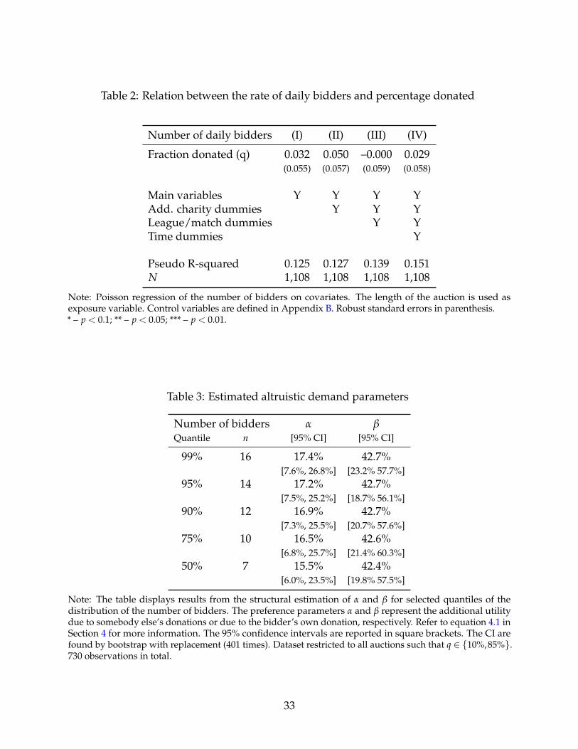
Table 2: Relation between the rate of daily bidders and percentage donated

Number of daily bidders (I) (II) (III) (IV)

Fraction donated (q) 0.032 0.050 –0.000 0.029(0.055) (0.057) (0.059) (0.058)

Main variables Y Y Y YAdd. charity dummies Y Y YLeague/match dummies Y YTime dummies Y

Pseudo R-squared 0.125 0.127 0.139 0.151N 1,108 1,108 1,108 1,108

Note: Poisson regression of the number of bidders on covariates. The length of the auction is used asexposure variable. Control variables are defined in Appendix B. Robust standard errors in parenthesis.* – p < 0.1; ** – p < 0.05; *** – p < 0.01.

Table 3: Estimated altruistic demand parameters

Number of bidders α βQuantile n [95% CI] [95% CI]

99% 16 17.4% 42.7%[7.6%, 26.8%] [23.2% 57.7%]

95% 14 17.2% 42.7%[7.5%, 25.2%] [18.7% 56.1%]

90% 12 16.9% 42.7%[7.3%, 25.5%] [20.7% 57.6%]

75% 10 16.5% 42.6%[6.8%, 25.7%] [21.4% 60.3%]

50% 7 15.5% 42.4%[6.0%, 23.5%] [19.8% 57.5%]

Note: The table displays results from the structural estimation of α and β for selected quantiles of thedistribution of the number of bidders. The preference parameters α and β represent the additional utilitydue to somebody else’s donations or due to the bidder’s own donation, respectively. Refer to equation 4.1 inSection 4 for more information. The 95% confidence intervals are reported in square brackets. The CI arefound by bootstrap with replacement (401 times). Dataset restricted to all auctions such that q ∈ {10%,85%}.730 observations in total.

33

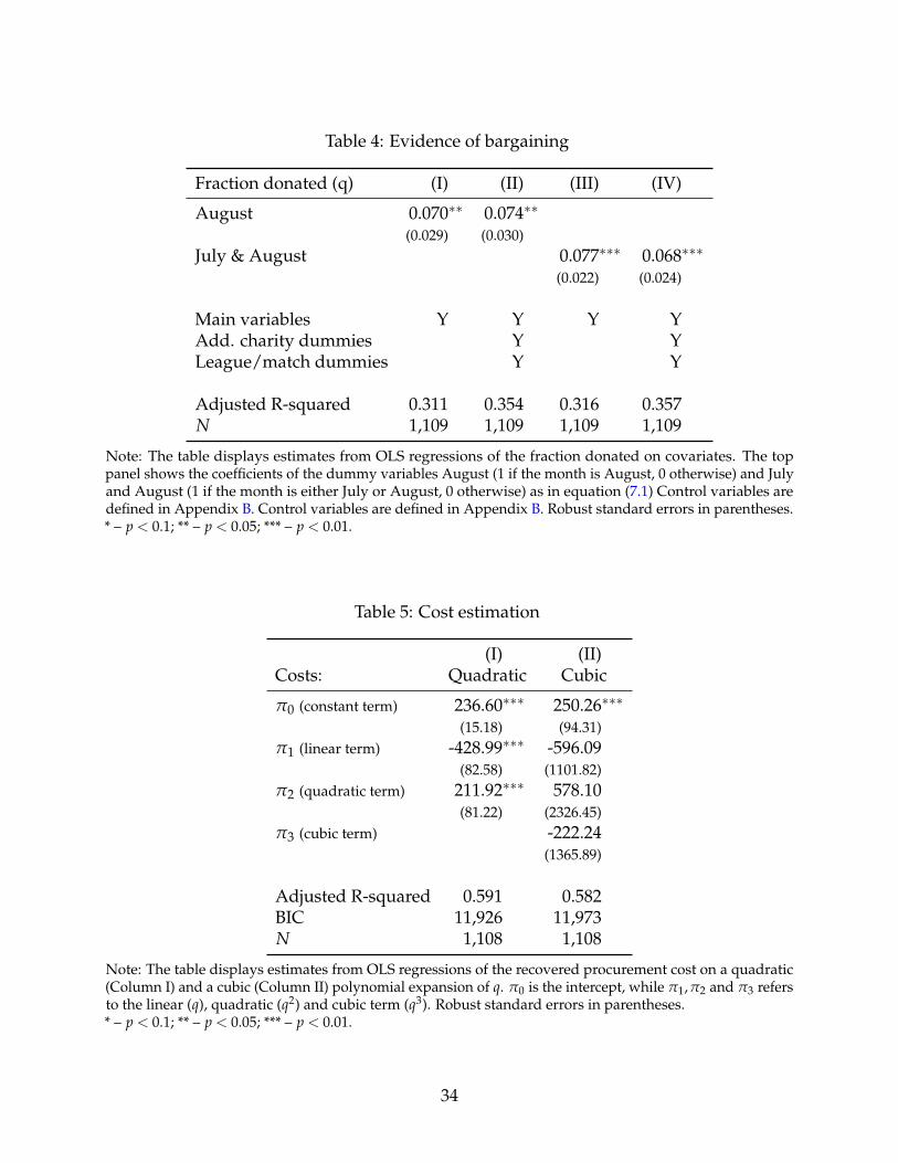
Table 4: Evidence of bargaining

Fraction donated (q) (I) (II) (III) (IV)

August 0.070∗∗ 0.074∗∗

(0.029) (0.030)July & August 0.077∗∗∗ 0.068∗∗∗

(0.022) (0.024)

Main variables Y Y Y YAdd. charity dummies Y YLeague/match dummies Y Y

Adjusted R-squared 0.311 0.354 0.316 0.357N 1,109 1,109 1,109 1,109

Note: The table displays estimates from OLS regressions of the fraction donated on covariates. The toppanel shows the coefficients of the dummy variables August (1 if the month is August, 0 otherwise) and Julyand August (1 if the month is either July or August, 0 otherwise) as in equation (7.1) Control variables aredefined in Appendix B. Control variables are defined in Appendix B. Robust standard errors in parentheses.* – p < 0.1; ** – p < 0.05; *** – p < 0.01.

Table 5: Cost estimation

(I) (II)Costs: Quadratic Cubic

π0 (constant term) 236.60∗∗∗ 250.26∗∗∗

(15.18) (94.31)π1 (linear term) -428.99∗∗∗ -596.09

(82.58) (1101.82)π2 (quadratic term) 211.92∗∗∗ 578.10

(81.22) (2326.45)π3 (cubic term) -222.24

(1365.89)

Adjusted R-squared 0.591 0.582BIC 11,926 11,973N 1,108 1,108

Note: The table displays estimates from OLS regressions of the recovered procurement cost on a quadratic(Column I) and a cubic (Column II) polynomial expansion of q. π0 is the intercept, while π1,π2 and π3 refersto the linear (q), quadratic (q2) and cubic term (q3). Robust standard errors in parentheses.* – p < 0.1; ** – p < 0.05; *** – p < 0.01.

34

Figure 1: Number of auctions by percentage donated

1

171

115

1 2

53

195

110

560

324

2

50

1

Non−Standard

Auctions

0

100

200

300

400

500

600

0 10 15 20 30 70 72 78 80 85 86 88 90 93 100Percentage donated %

Num

ber

of A

uctions

Note: The barplot displays the number of auctions available in the dataset by percentage donated. The plotincludes only auctions of items for a price in (e 100, e 1,000) with reserve price was greater than 0, at leasttwo bidders and minimum increment not greater than e 25. There are 1,189 auctions in total. Charitystarsgenerally withholds at least 15% of the final price and therefore all auctions whose percentage donated isabove 85% are excluded from the analyses as these are special one-off charitable events (black columns).However, non-standard auctions are also counted in when computing variables such as those accountingfor the number of auctions hold for the same player or for the same team in the past two and three weeksrespectively.

35

Figure 2: The impact of a change in q on bids and revenues

(a) Derivative of the bid with respect to α

0 line

−30

−10

10

30

50

0 25 50 75 100Private values

Deri

vative

of bid

w.r

.t.

q

α = 0.7, β = 0.9, σ = 20 α = 0.7, β = 0.5, σ = 20 α = 0.7, β = 0.5, σ = 80

(b) The revenue maximizing donation (qR)

revenue maximizing q

0

0.1

0.2

0.3

0.4

0.5

0

10

20

30

40

50

0.00 0.25 0.50 0.75 1.00Fraction donated (q)

Ela

sticity,

q/(

1−

q) N

et R

evenues

Elasticityq / (1−q)

Net Revenues

Note: Panel a. The figure reports the analytical derivative of the bid function equation 4.2 w.r.t. q. q = 85%and F(·) is a truncated normal in [0,100] with mean 50 and standard deviation σ. Panel b. The figure showsthe optimal percentage donated (qR) obtained at the intersection of the elasticity of the expected winning bidwith respect to q and the curve q/(1− q). Values of the elasticity and q/(1− q) (solid and dotted curves) areon the left vertical axis. The right axis shows the net revenues (dashed curve) (or second-highest bid times(1− q)): (1− q)

∫v b(v)dF(2)

(n)(v)). The distribution of values F(v) is uniform on [0,100], α = 0.5, β = 0.7 andthere are two bidders.

Figure 3: Out-of-sample validation

0.000

0.002

0.004

0.006

0 250 500 750 1000Private Value

pdf

q = 10%q = 78%

Note: The plot compares the density of the private values estimated from the structural model employingdata from auctions with q = {10%,85%} and the density of the private values obtained projecting thethree-step estimation procedure on the q = 78% auctions. The null hypothesis (equality) cannot be rejectedat standard level (p-value: 0.1874). The estimations assume n = 16, a Gaussian kernel and Silverman’srule-of-thumb bandwidth (Silverman, 1986). The density f (v) is approximated using a cubic spline.

36

Figure 4: Charity premium

(a) Gross revenues and charity markup

0

100

200

300

400

500

0

5

10

15

20

25

0.00 0.25 0.50 0.75 1.00Fraction donated (q)

Tra

nsaction P

rice (

EU

R)

Mark

up (%

)

CharityNon−Charity

Charity Markup

(b) Net revenues and elasticity of demand

0

0.1

0.2

0.3

0.4

0.5

0

100

200

300

400

500

0.00 0.25 0.50 0.75 1.00Fraction donated (q)

Ela

sticity,

q/(

1−

q)

Net R

evenues (E

UR

)

Elasticityq / (1−q)

Net Revenues

Note: Panel a. The plot displays the expected gross revenues to Charitystars at the estimated primitives(solid line), the revenues from a similar second-price non-charity auction (dotted line), and the charitymarkup (dashed line, right axis). Panel b. The plot displays the expected net revenues (dashed line, rightaxis), the elasticity of the winning bid (solid line, left axis) and the ratio q/(1− q) (dotted line, left axis)for varying levels of q. The density f (v) and the distribution F(v) are approximated using a cubic spline.Revenues assume that the number of potential bidders is 7 in both plots.

37

Figure 5: Optimal donation

(a) Optimal fraction donated

−600

−500

−400

−300

−200

−100

0

0.00 0.25 0.50 0.75 1.00Fraction donated (q)

MR

, M

C (

EU

R)

M Net RevenueMC − Quadratic

MC − Cubic

(b) Optimal profits

median donation

−25

0

25

50

75

100

125

150

0.00 0.25 0.50 0.75 1.00Fraction donated (q)

Pro

fits

(E

UR

)

Note: Panel a. The plot displays the optimal fraction donated as the intersection of marginal costs (dottedand dashed lines) and net benefits (solid line). The marginal costs are estimated using quadratic polynomials(dotted line) and cubic polynomials (dashed line). Panel b. The plot displays how profits change with thefraction donated (q). The vertical line at 85% indicate the median donation by Charitystars. The density f (v)and the distribution F(v) are approximated using a cubic spline. Profits are computed as net revenues minuscosts as in the quadratic polynomials case. Marginal revenues assume that the number of potential biddersis 7 in both plots.

38

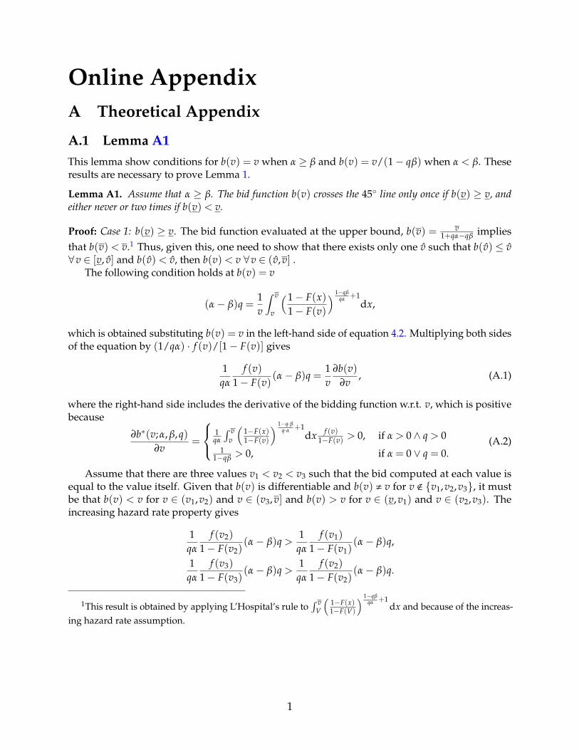
Online AppendixA Theoretical Appendix

A.1 Lemma A1This lemma show conditions for b(v) = v when α ≥ β and b(v) = v/(1− qβ) when α < β. Theseresults are necessary to prove Lemma 1.

Lemma A1. Assume that α ≥ β. The bid function b(v) crosses the 45◦ line only once if b(v) ≥ v, andeither never or two times if b(v) < v.

Proof: Case 1: b(v) ≥ v. The bid function evaluated at the upper bound, b(v) = v1+qα−qβ implies

that b(v) < v.1 Thus, given this, one need to show that there exists only one v such that b(v) ≤ v∀v ∈ [v, v] and b(v) < v, then b(v) < v ∀v ∈ (v,v] .

The following condition holds at b(v) = v

(α− β)q =1v

∫ v

v

(1− F(x)1− F(v)

) 1−qβqα +1

dx,

which is obtained substituting b(v) = v in the left-hand side of equation 4.2. Multiplying both sidesof the equation by (1/qα) · f (v)/[1− F(v)] gives

1qα

f (v)1− F(v)

(α− β)q =1v

∂b(v)∂v

, (A.1)

where the right-hand side includes the derivative of the bidding function w.r.t. v, which is positivebecause

∂b∗(v;α, β,q)∂v

=

1qα

∫ vv

(1−F(x)1−F(v)

) 1−q·βq·α +1

dx f (v)1−F(v) > 0, if α > 0∧ q > 0

11−qβ > 0, if α = 0∨ q = 0.

(A.2)

Assume that there are three values v1 < v2 < v3 such that the bid computed at each value isequal to the value itself. Given that b(v) is differentiable and b(v) , v for v < {v1,v2,v3}, it mustbe that b(v) < v for v ∈ (v1,v2) and v ∈ (v3,v] and b(v) > v for v ∈ (v,v1) and v ∈ (v2,v3). Theincreasing hazard rate property gives

1qα

f (v2)

1− F(v2)(α− β)q >

1qα

f (v1)

1− F(v1)(α− β)q,

1qα

f (v3)

1− F(v3)(α− β)q >

1qα

f (v2)

1− F(v2)(α− β)q.

1This result is obtained by applying L’Hospital’s rule to∫ v

V

(1−F(x)1−F(V)

) 1−qβqα +1

dx and because of the increas-ing hazard rate assumption.

1

Because equation A.1 must hold at v1,v2 and v3, it implies that

∂b(v2)∂v2

∂b(v1)∂v1

>v2

v1> 1 and

∂b(v3)∂v3

∂b(v2)∂v2

>v3

v2> 1,

a contradiction. While the ratio of the derivative at v2 and v1 must be larger than 1, as the curveintersects the 45◦ line from below the line, this cannot happen at v3 and v2, because the intersectionhappens from above the line. The bid function crosses the 45◦ line at v2 from below, while it crossesthe same line from above at v3, implying

∂b(v3)

∂v3<

∂b(v2)

∂v2.

Figure A1b provides a graphical representation. Because v1,v2 and v3 are arbitrary values, the proofholds for all v. Given that b(v) ≥ v, b(v) < v and because b(v) cannot cross the 45◦ line more thantwice without violating the increasing hazard rate property, it must be that b(v) = v at most once.

Case 2: b(v) < v. This case follows immediately from the previous derivation, given that b(v)cannot cross the 45◦ line more than twice without violating the increasing hazard rate assumption.This implies that b(v) = v for either two values v1 and v2 or no value at all. In this case, in order torespect the increasing hazard rate property, the bid function meets the diagonal line from below atthe first cutoff and from above at the second cutoff, making a cutoff like v3 infeasible. �

A.2 Proof of Lemma 1Bids are- increasing in q if β ≥ α;- decreasing in q in the interval (v,v], where v ∈ [v,v], if α > β.

Proof: Assume q > 0 and let α = q · α and β = q · β. First we analyze the derivative of b(v) w.r.t. qwhen α = 0, which is:

∂b∗(v;α = 0, β,q)∂q

=βv

(1− β)2> 0.

The derivative in this case is always positive as β < 1 and q < 1, meaning that bids increase in q.Turn now to the derivative with respect to q when α is positive. This proof has multiple steps.

(step 1) I establish that for β ≥ α > 0 the bid is increasing in q ∀v. (step 2) I focus on the remainingcase (β < α) and show that the derivative of the bid w.r.t. q can have both positive and negativevalues. (step 2.a) I show that, at the value such that the derivative is zero (called v), if the bid islarger than the value the derivative of b(v) w.r.t. q is decreasing. (step 2.b) In the final step, I showconditions for the uniqueness of v.

Step 1: β ≥ α > 0 . The derivative of equation 4.2 w.r.t. q for α > 0 is

∂b∗(v;α > 0, β,q)∂q

=

∫ vv

(1−F(x)1−F(v)

) 1+α−βα(− α(1+α−β)

α2 log 1−F(x)1−F(v) − (α− β)

)dx− (α− β)v

(1 + α− β)2. (A.3)

An application of the L’Hospital’s Rule shows that the integral is continuous and finite everywherewith respect to x. Inspection of this equation reveals that is positive if β ≥ α. Therefore, bids are

2

increasing in q if β > α for all v.

Step 2: 0 < α < β . Under this configuration, equation A.3 crosses the x-axis at v s.t. ∂b(v)∂q |v=v = 0.

Rewriting equation A.3 and evaluating it at v yields

−∫ v

v

(1− F(x)1− F(v)

) 1+α−βα α(1 + α− β)

α2 log1− F(x)1− F(v)

dx = (α− β)

v +∫ v

v

(1− F(x)1− F(v)

) 1−βα +1

dx

∣∣∣∣∣v=v

= (α− β)(1 + α− β)b(v).(A.4)

where the second line replaces the expression to the right-hand side with the optimal bid functionin equation 4.2. Thus, equation A.3 can be either positive or negative.

Step 2.a. This step shows that equation A.3 is decreasing at v if b(v) ≥ v. Given that the right-handside of equation A.4 is increasing in v everywhere, it will also be increasing in v at v. To show thatthere is at most one v, it suffices to show that the left-hand side is a decreasing function of v, at v.The derivative of the left-hand side w.r.t. v is

−∫ v

v

(1− F(x)1− F(v)

) 1−βα +1

α1 + α− β

α2

(1 +

1 + α− β

αlog

1− F(x)1− F(v)

)dx

f (v)1− F(v)

, (A.5)

while the derivative of the right-hand side can be rewritten as

(α− β)(1 + α− β)

α

(b(v)(1 + α− β)− v

)f (v)

1− F(v). (A.6)

Putting together equation A.5 and equation A.6 and using equation A.4 to rewrite equation A.5 interms of bids and values, equation A.3 is decreasing at v if

−(b(v)(1 + α− β)− v

)α

1 + α− β

α2 + (α− β)(1 + α− β)2

αb(v)

≤ (α− β)(1 + α− β)

α

(b(v)(1 + α− β)− v

)⇒ b(v) ≥ v.

This means that equation A.3 is positive at the left of v and negative to the right of v. Therefore,as long as the equilibrium bid at the cut-off value v is greater than the cut-off itself, bids will bedecreasing in q for all v > v, if α > β.

Step 2.b. When α > β, the limit of equation A.3 for v→ v is negative. In fact, under the increasinghazard rate condition (Assumption 1) applying L’Hospital’s rule to the first term (in the numerator)of equation A.3 yields

limv→v

∫ vv (1− F(x))

1+α−βα

(− α(1+α−β)

α2 log 1−F(x)1−F(v) − (α− β)

)dx

(1 + α− β)2 (1− F(v))1+α−β

α

= 0,

while the limit of the remaining part is limv→v−(α− β)v = −(α− β)v < 0. There are two cases: inCase 1 v is unique and in Case 2 either v does not exist or there are two v.

Step 2.b: Case 1. The first case assumes b(v) ≥ v. To show that v is unique I merge two results: (i)

3

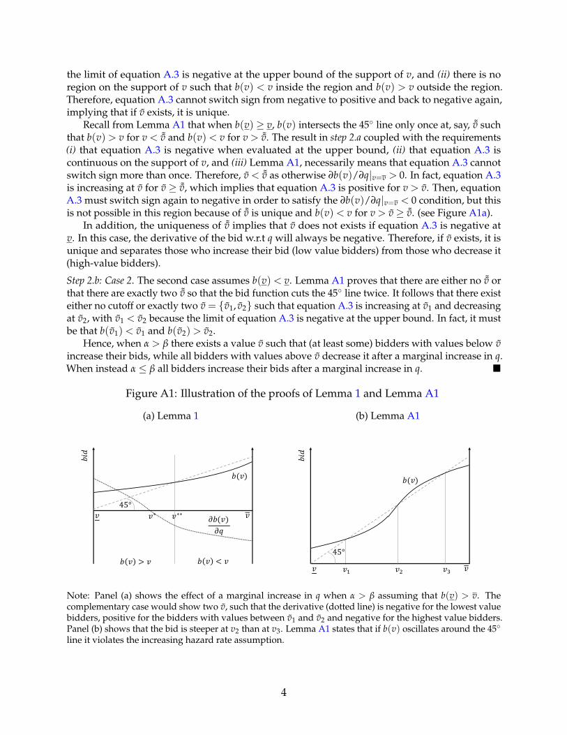
the limit of equation A.3 is negative at the upper bound of the support of v, and (ii) there is noregion on the support of v such that b(v) < v inside the region and b(v) > v outside the region.Therefore, equation A.3 cannot switch sign from negative to positive and back to negative again,implying that if v exists, it is unique.

Recall from Lemma A1 that when b(v) ≥ v, b(v) intersects the 45◦ line only once at, say, ˜v suchthat b(v) > v for v < ˜v and b(v) < v for v > ˜v. The result in step 2.a coupled with the requirements(i) that equation A.3 is negative when evaluated at the upper bound, (ii) that equation A.3 iscontinuous on the support of v, and (iii) Lemma A1, necessarily means that equation A.3 cannotswitch sign more than once. Therefore, v < ˜v as otherwise ∂b(v)/∂q|v=v > 0. In fact, equation A.3is increasing at v for v ≥ ˜v, which implies that equation A.3 is positive for v > v. Then, equationA.3 must switch sign again to negative in order to satisfy the ∂b(v)/∂q|v=v < 0 condition, but thisis not possible in this region because of ˜v is unique and b(v) < v for v > v ≥ ˜v. (see Figure A1a).

In addition, the uniqueness of ˜v implies that v does not exists if equation A.3 is negative atv. In this case, the derivative of the bid w.r.t q will always be negative. Therefore, if v exists, it isunique and separates those who increase their bid (low value bidders) from those who decrease it(high-value bidders).

Step 2.b: Case 2. The second case assumes b(v) < v. Lemma A1 proves that there are either no ˜v orthat there are exactly two ˜v so that the bid function cuts the 45◦ line twice. It follows that there existeither no cutoff or exactly two v = {v1, v2} such that equation A.3 is increasing at v1 and decreasingat v2, with v1 < v2 because the limit of equation A.3 is negative at the upper bound. In fact, it mustbe that b(v1) < v1 and b(v2) > v2.

Hence, when α > β there exists a value v such that (at least some) bidders with values below vincrease their bids, while all bidders with values above v decrease it after a marginal increase in q.When instead α ≤ β all bidders increase their bids after a marginal increase in q. �

Figure A1: Illustration of the proofs of Lemma 1 and Lemma A1

(a) Lemma 1

𝑣𝑣∗∗

𝑏(𝑣)

𝑣45°

𝑏 𝑣 > 𝑣 𝑏 𝑣 < 𝑣

𝜕𝑏(𝑣)

𝜕𝑞

𝑣∗

𝑏𝑖𝑑

(b) Lemma A1

𝑣" 𝑣𝑣# 𝑣$

𝑏(𝑣)

𝑣

45°

𝑏𝑖𝑑

Note: Panel (a) shows the effect of a marginal increase in q when α > β assuming that b(v) > v. Thecomplementary case would show two v, such that the derivative (dotted line) is negative for the lowest valuebidders, positive for the bidders with values between v1 and v2 and negative for the highest value bidders.Panel (b) shows that the bid is steeper at v2 than at v3. Lemma A1 states that if b(v) oscillates around the 45◦

line it violates the increasing hazard rate assumption.

4

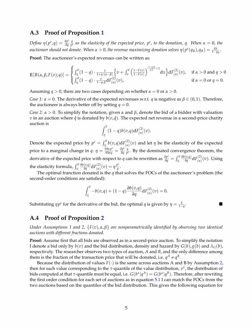
A.3 Proof of Proposition 1

Define η(pe,q) = ∂pe

∂qqpe as the elasticity of the expected price, pe, to the donation, q. When α = 0, the

auctioneer should not donate. When α > 0, the revenue maximizing donation solves η(pe(qR),qR) =qR

1−qR.

Proof: The auctioneer’s expected revenues can be written as:

E[R(α, β, F(v);q)] =

∫ v

v (1− q) · 11+q·(α−β)

{v +

∫ vv

(1−F(x)1−F(v)

) 1−q·βq·α +1

dx}

dF(2)(n)(v), if α > 0 and q > 0∫ v

v (1− q) · v1−q·β dF(2)

(n)(v), if α = 0 or q = 0.

Assuming q > 0, there are two cases depending on whether α = 0 or α > 0.

Case 1: α = 0. The derivative of the expected revrenues w.r.t. q is negative as β ∈ (0,1). Therefore,the auctioneer is always better off by setting q = 0.

Case 2: α > 0. To simplify the notation, given α and β, denote the bid of a bidder with valuationv in an auction where q is donated by b(v, q). The expected net revenue in a second-price charityauction is ∫ v

v(1− q)b(v,q)dF(2)

(n)(v).

Denote the expected price by pe =∫ v

v b(v,q)dF(2)(n)(v) and let η be the elasticity of the expected

price to a marginal change in q: η = ∂ ln pe

∂ lnq = ∂pe

∂qqpe . By the dominated convergence theorem, the

derivative of the expected price with respect to q can be rewritten as ∂pe

∂q =∫ v

v∂b(v,q)

∂q dF(2)(n)(v). Using

the elasticity formula,∫ v

v∂b(v,q)

∂q dF(2)(n)(v) = η

pe

q .The optimal franction donated is the q that solves the FOCs of the auctioneer’s problem (the

second-order conditions are satisfied):∫ v

v−b(v,q) + (1− q)

∂b(v,q)∂q

dF(2)(n)(v) = 0.

Substituting ηpe for the derivative of the bid, the optimal q is given by η = q1−q . �

A.4 Proof of Proposition 2Under Assumptions 1 and 2, {F(v),α, β} are nonparametrically identified by observing two identicalauctions with different fractions donated.

Proof: Assume first that all bids are observed as in a second-price auction. To simplify the notationI denote a bid only by b(v) and the bid distribution, density and hazard by G(b), g(b) and λG(b),respectively. The researcher observes two types of auction, A and B, and the only difference amongthem is the fraction of the transaction price that will be donated, i.e. qA , qB.

Because the distribution of values F(·) is the same across auctions A and B by Assumption 2,then for each value corresponding to the τ-quantile of the value distribution, vx, the distribution ofbids computed at that τ-quantile must be equal, i.e. G(bx|qA) = G(bx|qB). Therefore, after rewritingthe first order condition for each set of auctions as in equation 5.1 I can match the FOCs from thetwo auctions based on the quantiles of the bid distribution. This gives the following equation for

5

each quantile of vx:

vAx − vB

x = bAx − bB

x + (α− β) · (qA · bAx − qB · bB

x )− α · (qA · λG(bAx )− qB · λG(bB

x )), (A.7)

where G(bx) = G(bAx ) = G(bB

x ). Since vAx − vB

x = 0, eq. A.7 can be rewritten in matrix notation as

∆(bx) = Bx ×[

α− β−α

], (A.8)

where ∆(bx) = −(bAx − bB

x ) and Bx is the matrix [qAbAx − qBbB

x ; qA · λG(bAx )− qB · λG(bB

x )].The matrix Bx has full rank because the two columns are linearly independent. To prove

this assume to the converse that Bx is not invertible and therefore that its columns are linearlydependent (i.e. bx = k · λG(bx) for both auctions A and B). It follows that G(bx) = 1− bx · g(bx)/kfor a constant k > 0. Note that k must be positive because otherwise G(bx) > 1 as g(bx) ≥ 0,∀bx.The previous differential equation admits a solution g(bx) = c · (bx)−(k+1), where c is an integrationconstant. Thus, G(bx) = 1− c · (bx)−k/k. Evaluating the CDF at bx = 0 yields G(0) = −∞, ∀k > 0.Moreover, the inverse hazard rate

λG(bx) =1− 1 + c · (bx)−k/k

c · (bx)−(k+1)=

bx

kfor k > 0,

is increasing in bx. This implies that

1− F(vx)

f (vx)=

1− G(b(vx))

g(b(vx)) · b′(vx)=

1k

b(vx)

b′(vx),

which is an increasing function because (i) the optimal bidding function b(v) is increasing in theprivate value vx and (ii) the bidding function b(vx) maximizes a bidder’s utility (b′′(vx) ≤ 0). Thismeans that the inverse hazard rate is not decreasing and that therefore b(vx) is not a best responsefor vx. This is a contradiction, which proves that the columns in Bx are not linearly dependent andthat Bx is invertible.2 Given that Bx has full rank, α, β and F(v) are nonparametrically identified.

To extend this result to Charitystars’s auctions, note that the distribution of the winning bid(Gw(b)) is identified from the data. In equilibrium, the distribution of the winning bid is equalto the distribution of the second-highest bid (Gw(b) = G2

(n)(b)). Therefore, G(b) is found as theroot (in [0,1]) of Gw(b)− nG(b)n−1 + (n− 1)G(b)n. The FOCs equation 5.1 can then be written foreach {α, β}. Therefore, one can apply the same logic shown above, and identify α, β. Finally, withknowledge of the couple {α, β}, the distribution of private values, F(v), is identified from the FOCsequation 5.1 of the winning bids. �

A.5 Proof of Corollary 1Corollary 1. α, β and F(v) are also nonparametrically identified when the dataset includes more than 2types of auctions.

Proof: To simplify the notation I denote a bid only by b(v) and the bid distribution, density and

2If k = 1, then g(bx) = 0 for bx < 0 and g(bx) > 0 for bx ≥ 0. Therefore g(·) is the Dirac delta function,which is not differentiable and does not admit a decreasing inverse hazard rate. In turn, given that F(v) =G(b(v)), the non-differentiability of G(·) implies that also the distribution of values F(·) is not differentiable,a contradiction.

6

hazard by G(b), g(b) and λG(b), respectively. Assume that q has dimension KC and that Kx quantilesof the distribution of values are observed. The FOC equation 5.1 in matrix notation becomes

VKx × KC

= (α− β)× BKx × KC

× QC

KC × KC

+ BKx × KC

−α× ΛKx × KC

× QC

KC × KC

, (A.9)

where V is a matrix of dimension Kx × KC displaying the value vx for the x−quantile (row) inauction of type C (column), and 0 otherwise. Similarly, QC is a diagonal matrix with entries equalto the percentage donated qC and 0. The other matrices are defined as:

B =

b10 b2

0 . . . bKC0

......

. . ....

b11 b2

1 . . . bKC1

, Λ =

λ1G(b

10) λ2

G(b20) . . . λKC

G (bKC0 )

......

. . ....

λ1G(b

11) λC2

G (b21) . . . λKC

G (bKC1 )

,

where superscripts indicate that the franction donated is equal to qj for j ∈ [1,KC] and subscriptsindicate the x− quantiles of the distribution of values or bids.

There exists a projection M (with rank KC − 1) such that V ×M = 0. Postmultiplying equationA.9 by M and moving terms, the following equation represents the FOC where the dependentvariable is a known object

−B×M = (α− β)× B×QC ×M− α×Λ×QC ×M.

After stacking the matrices in vectors, the last equation can be represented by the system ofequations

y =[b l

]×[

α− β−α

],

where y = vec(−B× M),b = vec(B× QC × M), l = vec(Λ× QC × M), and vec(·) indicates thevectorization of the matrices in parentheses.

Nonparametric identification requires showing that b and l are linearly independent, whichfollows directly from the argument in the proof of Proposition 2 in Appendix A.4. Hence, b and lare not linearly dependent, establishing identification of α, β and F(v). �

A.6 The Bargaining ProblemThis section provides a micro foundation to the condition for the optimal q∗ in equation 7.2 inSection 7. The surplus to the firm is the difference of the net revenues (1− q)p and the procurementcost κ. For simplicity, κ does not vary with q. Item providers (i.e., charities and celebrities) care forthe amount that is ultimately donated. For simplicity they incur no cost in giving the item. Thebargaining weights are ω for the firm and 1−ω for the provider. In this bargaining framework, qmaximizes (

(1− q)pe − κ)ω · (qpe + κ)1−ω,

where pe denotes the expected highest price, and is a function of the distribution of values, thecharity parameters (i.e., α and β), the number of bidders and q. The first-order condition with

7

respect to q can be rearranged to obtain

− pe

((1−ω) ((1− q) pe − κ)

ωκ + q ((1− q) pe − κ)

)=

1− qq

ηpe − pe, (A.10)

where η is the elasticity of the expected price to a change in q. The right-hand side is the same as inequation 7.2, while the left-hand side is a function of the primitives.

The left-hand side can be interpreted as the marginal cost of the monopolist problem as inSection 7 (c′(q)). When ω = 1, all bargaining power is in the hand of Charitystars, the left-hand sidebecomes 0, and the optimal q∗ solves η = q

1−q , as in the revenue maximization case (see Proposition1). Because there is no bargaining, setting a greater q does not yield any cost savings (i.e., c′(q) = 0).Since Charitystars sets the reserve price to break even, the fraction in parenthesis on the left-handside is always positive (i.e., (1− q)pe > κ). Therefore when 0≤ ω < 1, the left-hand side is negative,implying negative marginal costs in the model in Section 7.

Finally, the left-hand side in equation A.10 can be rearranged by adding and subtracting 1/q inthe term in parentheses

−pe

(− ω

qκ + q ((1− q) pe − κ)

ωκ + q ((1− q) pe − κ)+

1q

)≈ − pe

q(1−ω),

which gives a clean interpretation of the marginal cost in terms of the bargaining weight andprimitives of the model.

8

B Data DescriptionThe data was collected using a Python script that searched a list of keywords across the pagesdedicated to soccer items on the company website, available at http://www.charitystars.com.The script would gather all the available information regarding the auction, the charity, the listingand the bid history. This information was augmented with data from other sources. For example, asimilar python script was used to recover footballers’ quality scores from a renowned videogame(FIFA). Information on each charity’s mission was obtained from both Charitystars as well as eachcharity’s website.

The analysis considers only a subset of the available auctions (see Section 2), according to thefollowing conditions: (i) transaction prices higher than the reserve price, (ii) reserve prices greaterthan zero, (iii) two or more bidders, (iv) minimum increment is within e 25 and (v) maximumdonation of 85% of the final price.

B.1 Description of the VariablesThe regressions in Section 2 and in the Appendix display only some of the actual variables used inthe analyses due to space limitations. These variables were distinguished in four groups based ontheir relevance.

1. Main Variables: these are the variables used in all regression tables and in the structural model.They are listed in Table B1 and their meaning is described by their label. Some variableswhose meaning is not immediately clear are described in the following list:

• The variable Length counts the number of days between the first bid and the closingdate (the listing date of the auction is unknown).

• The dummy Extended time is 1 if two or more bidders placed a bid in the last minutes ofthe auction. In this case the time is extended until all but 1 bidders drop out

• Auctions within 3 weeks (same team) counts the number of auctions listing jerseys of thesame team as the one of the auctioned item. It only includes auctions within a 3 weekwindow from the end of the auction. It considers all auctions not only those with finalprice larger than e 100 and smaller than e 1000.

• Auctions up to 2 weeks ago (same player/team) counts the number of auctions for a jerseyworn by the same player playing with the same team in the same year as the match ofthe jersey that is auctioned. It considers all the listings up to 2 weeks from the end of theauction (Charitystars’s auctions last between 1 and 2 weeks). It considers all auctionsnot only those with final price larger than e 100 and smaller than e 1000.

• Count auctions same charity is a progressive count of the number of listings for eachcharity.

• The dummy Player belongs to FIFA 100 list is 1 if the player is in the FIFA 100 list (the listof the best soccer players ever).

• The variable Number of goals scored is equal to the number of goals scored by the playerwith the auctioned jersey in a particular match if this number is mentioned in thecontent of the listing. It is zero otherwise.

• The dummy Player belongs to an important team is 1 if the player plays for one of the fol-lowing teams (alphabetic order): AC Milan, Argentina, Arsenal FC, AS Roma, Atletico

9

de Madrid, Barcelona FC, Bayern Munich, Belgium, Borussia Dortmund, Brazil, ChelseaFC, Colombia, England, FC Internazionale, France, Germany, Italia, Juventus FC, Liver-pool FC, Manchester City, Manchester United, Netherlands, PSG, Real Madrid, SevillaFC, Spain, SS Lazio, SSC Napoli, Uruguay. 3

2. Add. Charity Dummies: this group includes dummies for heterogeneity across charities basedon the mission of each charity. These dummies are not exclusive bins as most charities domore than only one activity. There are 101 different charities in total. The dummy variablesused

• Helping disables individuals for charities involved in assistance to disable subjects.

• Infrustructures in developing countries for charities building infrastructures in developingcountries.

• Healthcare for charities dealing with healthcare and health research.

• Humanitarian scopes in developing countries for charities helping people in situation ofpoverty and undernourishment.

• Children’s wellbeing for charities providing activities (e.g., education and sport) to theyouth.

• Neurodegenerative disorders for charities helping those suffering from neurodegenerativedisorders.

• Charity belongs to the soccer team are charities linked to a football team.

• Improving access to sport charities give opportunity of integration through sport activities.

• Italian charity.

• English charity.

3. League/Match Dummies: these are dummies for soccer league and match heterogeneity. Theyinclude:

• Dummies for each major competition (Champions League, Europa League, Serie A, ItalianCup, Premier League, La Liga, Copa del Rey, European Supercup, Italian Supercup, SpanishSupercup, UEFA European Championship, Qualifications to UEFA European Championship,World Cup, Qualification to the World Cup4).

• Dummies weather the listings mentions that the match was won (Won) and for unoffi-cial/replica jerseys which are not worn but only signed (Unofficial). There are only 79jerseys in the dataset that are replica, and they are all signed by the player.

4. Time Dummies: this group include Month dummies (12 variables) and Year dummies (2variables).

3In unreported analysis player quality was accounted also using the players’ evaluation from thevideogame FIFA. These variables do not affect prices significantly and are dropped.

4All remaining competitions are treated as friendly matches.

10

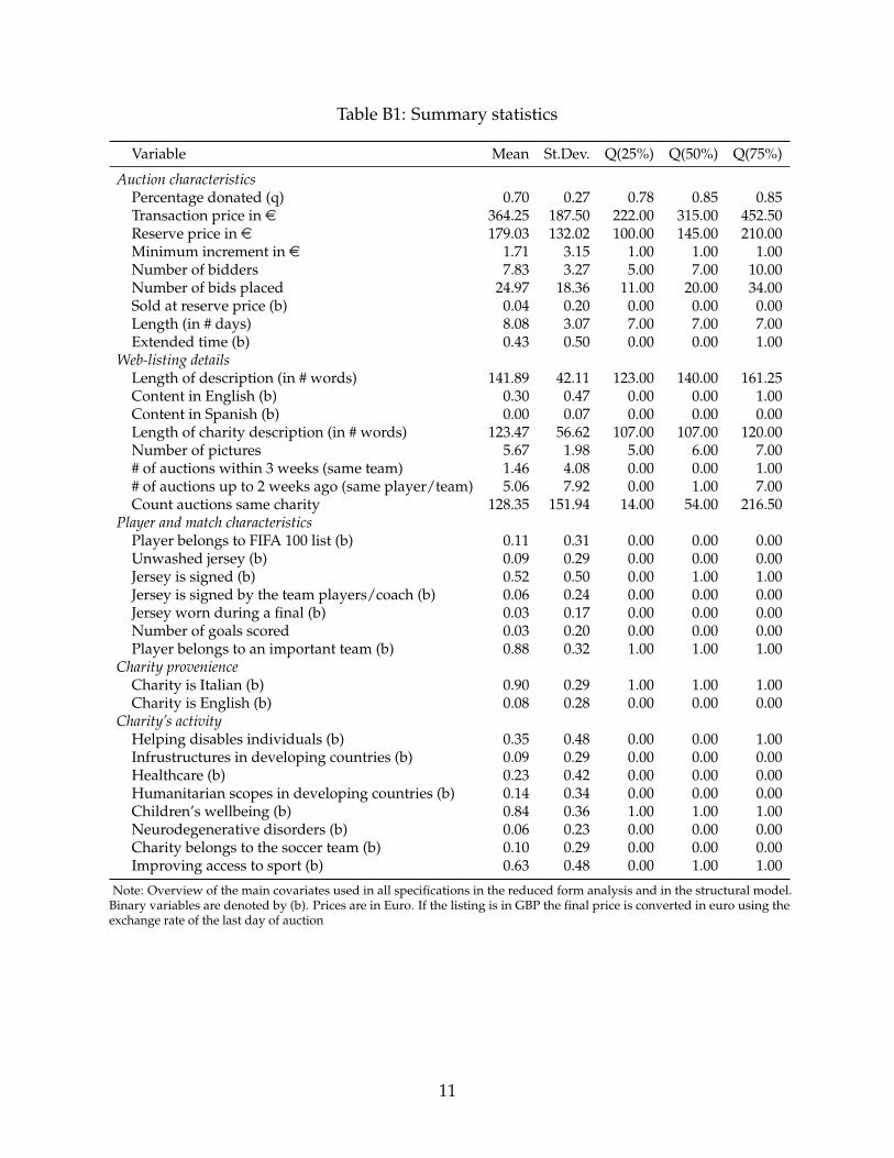
Table B1: Summary statistics

Variable Mean St.Dev. Q(25%) Q(50%) Q(75%)

Auction characteristicsPercentage donated (q) 0.70 0.27 0.78 0.85 0.85Transaction price in e 364.25 187.50 222.00 315.00 452.50Reserve price in e 179.03 132.02 100.00 145.00 210.00Minimum increment in e 1.71 3.15 1.00 1.00 1.00Number of bidders 7.83 3.27 5.00 7.00 10.00Number of bids placed 24.97 18.36 11.00 20.00 34.00Sold at reserve price (b) 0.04 0.20 0.00 0.00 0.00Length (in # days) 8.08 3.07 7.00 7.00 7.00Extended time (b) 0.43 0.50 0.00 0.00 1.00

Web-listing detailsLength of description (in # words) 141.89 42.11 123.00 140.00 161.25Content in English (b) 0.30 0.47 0.00 0.00 1.00Content in Spanish (b) 0.00 0.07 0.00 0.00 0.00Length of charity description (in # words) 123.47 56.62 107.00 107.00 120.00Number of pictures 5.67 1.98 5.00 6.00 7.00# of auctions within 3 weeks (same team) 1.46 4.08 0.00 0.00 1.00# of auctions up to 2 weeks ago (same player/team) 5.06 7.92 0.00 1.00 7.00Count auctions same charity 128.35 151.94 14.00 54.00 216.50

Player and match characteristicsPlayer belongs to FIFA 100 list (b) 0.11 0.31 0.00 0.00 0.00Unwashed jersey (b) 0.09 0.29 0.00 0.00 0.00Jersey is signed (b) 0.52 0.50 0.00 1.00 1.00Jersey is signed by the team players/coach (b) 0.06 0.24 0.00 0.00 0.00Jersey worn during a final (b) 0.03 0.17 0.00 0.00 0.00Number of goals scored 0.03 0.20 0.00 0.00 0.00Player belongs to an important team (b) 0.88 0.32 1.00 1.00 1.00

Charity provenienceCharity is Italian (b) 0.90 0.29 1.00 1.00 1.00Charity is English (b) 0.08 0.28 0.00 0.00 0.00

Charity’s activityHelping disables individuals (b) 0.35 0.48 0.00 0.00 1.00Infrustructures in developing countries (b) 0.09 0.29 0.00 0.00 0.00Healthcare (b) 0.23 0.42 0.00 0.00 0.00Humanitarian scopes in developing countries (b) 0.14 0.34 0.00 0.00 0.00Children’s wellbeing (b) 0.84 0.36 1.00 1.00 1.00Neurodegenerative disorders (b) 0.06 0.23 0.00 0.00 0.00Charity belongs to the soccer team (b) 0.10 0.29 0.00 0.00 0.00Improving access to sport (b) 0.63 0.48 0.00 1.00 1.00

Note: Overview of the main covariates used in all specifications in the reduced form analysis and in the structural model.Binary variables are denoted by (b). Prices are in Euro. If the listing is in GBP the final price is converted in euro using theexchange rate of the last day of auction

11

C Additional Tables

Table C1: Linearity of the relation between the logarithm of the transaction price andpercentage donated

(I) (II) (III) (IV)log(Transaction price) OLS Q(0.25) Q(0.50) Q(0.75)

Fraction donated (q) 0.212∗∗∗ 0.228∗∗∗ 0.305∗∗∗ 0.334∗∗∗

(0.046) (0.054) (0.089) (0.079)

F-test of equality with OLS (p-value) 0.762 0.299 0.124

Main variables Y Y Y Y

Adjusted/pseudo R-squared 0.502 0.353 0.326 0.315N 1,108 1,108 1,108 1,108

Note: The table displays estimates from OLS and quantile regressions of the logarithm of the transactionprice on covariates. The null hypothesis that the coefficient of the fraction donated (q) is the same in column(II), (III) and (IV) is not rejected at 0.429 levels (F-test = 0.85). The last three columns report Pseudo R-squaredin place of Adjusted R-squared. The coefficients of the quantile regressions are plotted in Appendix FigureD3. Control variables are defined in Appendix B. Robust standard errors in parenthesis.* – p < 0.1; ** – p < 0.05; *** – p < 0.01.

12

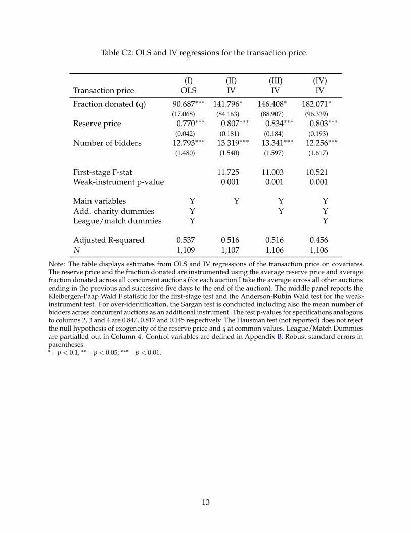
Table C2: OLS and IV regressions for the transaction price.

(I) (II) (III) (IV)Transaction price OLS IV IV IV

Fraction donated (q) 90.687∗∗∗ 141.796∗ 146.408∗ 182.071∗

(17.068) (84.163) (88.907) (96.339)Reserve price 0.770∗∗∗ 0.807∗∗∗ 0.834∗∗∗ 0.803∗∗∗

(0.042) (0.181) (0.184) (0.193)Number of bidders 12.793∗∗∗ 13.319∗∗∗ 13.341∗∗∗ 12.256∗∗∗

(1.480) (1.540) (1.597) (1.617)

First-stage F-stat 11.725 11.003 10.521Weak-instrument p-value 0.001 0.001 0.001

Main variables Y Y Y YAdd. charity dummies Y Y YLeague/match dummies Y Y

Adjusted R-squared 0.537 0.516 0.516 0.456N 1,109 1,107 1,106 1,106

Note: The table displays estimates from OLS and IV regressions of the transaction price on covariates.The reserve price and the fraction donated are instrumented using the average reserve price and averagefraction donated across all concurrent auctions (for each auction I take the average across all other auctionsending in the previous and successive five days to the end of the auction). The middle panel reports theKleibergen-Paap Wald F statistic for the first-stage test and the Anderson-Rubin Wald test for the weak-instrument test. For over-identification, the Sargan test is conducted including also the mean number ofbidders across concurrent auctions as an additional instrument. The test p-values for specifications analogousto columns 2, 3 and 4 are 0.847, 0.817 and 0.145 respectively. The Hausman test (not reported) does not rejectthe null hypothesis of exogeneity of the reserve price and q at common values. League/Match Dummiesare partialled out in Column 4. Control variables are defined in Appendix B. Robust standard errors inparentheses.* – p < 0.1; ** – p < 0.05; *** – p < 0.01.

13

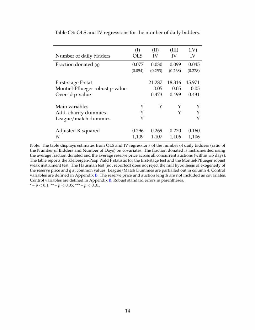
Table C3: OLS and IV regressions for the number of daily bidders.

(I) (II) (III) (IV)Number of daily bidders OLS IV IV IV

Fraction donated (q) 0.077 0.030 0.099 0.045(0.054) (0.253) (0.268) (0.278)

First-stage F-stat 21.287 18.316 15.971Montiel-Pflueger robust p-value 0.05 0.05 0.05Over-id p-value 0.473 0.499 0.431

Main variables Y Y Y YAdd. charity dummies Y Y YLeague/match dummies Y Y

Adjusted R-squared 0.296 0.269 0.270 0.160N 1,109 1,107 1,106 1,106

Note: The table displays estimates from OLS and IV regressions of the number of daily bidders (ratio ofthe Number of Bidders and Number of Days) on covariates. The fraction donated is instrumented usingthe average fraction donated and the average reserve price across all concurrent auctions (within ±5 days).The table reports the Kleibergen-Paap Wald F statistic for the first-stage test and the Montiel-Pflueger robustweak instrument test. The Hausman test (not reported) does not reject the null hypothesis of exogeneity ofthe reserve price and q at common values. League/Match Dummies are partialled out in column 4. Controlvariables are defined in Appendix B. The reserve price and auction length are not included as covariates.Control variables are defined in Appendix B. Robust standard errors in parentheses.* – p < 0.1; ** – p < 0.05; *** – p < 0.01.

14

Table C4: Evidence of bargaining: IV regressions

(I) (II) (III) (IV)Fraction donated (q) (OLS) (IV) (OLS) (IV)

August 0.074∗∗ 0.107∗∗∗

(0.030) (0.039)July & August 0.068∗∗∗ 0.112∗∗∗

(0.024) (0.034)

First-stage F-stat 10.480 9.613Weak-instrument p-value 0.022 0.004

Main variables Y Y Y YAdd. charity dummies Y Y Y YLeague/match dummies Y Y Y Y

Adjusted R-squared 0.354 0.270 0.357 0.187N 1,109 1,107 1,109 1,107

Note: The table displays estimates from OLS and IV regressions of the fraction donated on covariates. Thetop panel shows the coefficients of the dummy variables August (1 if the month is August, 0 otherwise) andJuly and August (1 if the month is either July or August, 0 otherwise) as in equation (7.1). The reserve priceand the number of bidders are instrumented using the average reserve price and the number of biddersacross all concurrent auctions (for each auction I take all the auctions ending in the previous and successivefive days to the end of the auction). The table reports the Kleibergen-Paap Wald F statistic for the first-stagetest and the Anderson-Rubin Wald test for the weak-instrument test. For over-identification (Sargan test)the average number of pictures across concurrent auctions (±5 days ) is also included as an additionalinstrument. The test p-value for specifications analogous to columns 2 and 4 are 0.166 and 0.221 respectively.League/Match Dummies are partialled out in columns 2 and 4. Control variables are defined in Appendix B.Robust standard errors in parentheses.* – p < 0.1; ** – p < 0.05; *** – p < 0.01.

Table C5: Nationalities of the top bidders

Italian UK France OtherEU

NorthAm China Asia East

AsiaRest

World Tot

Winner 561 74 41 119 62 130 35 28 59 1,10950.67% 6.67% 3.70% 9.92% 5.59% 11.72% 3.16% 2.52% 5.32% –

Second 604 79 28 113 51 117 33 26 58 1,10954.46% 7.12% 2.52% 10.20% 4.60% 10.55% 2.98% 2.34% 5.23% –

Total 1,165 153 69 232 113 247 68 54 117 –

Note: Nationalities of the top bidders by geographic area. “Rest of the World” includes also Unknownnationalities (12 winners and highest losers in total).

15

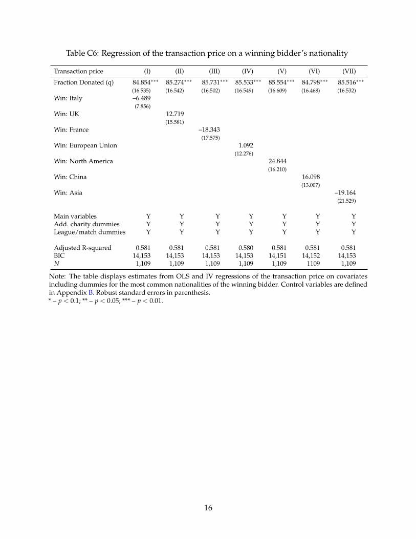
Table C6: Regression of the transaction price on a winning bidder’s nationality

Transaction price (I) (II) (III) (IV) (V) (VI) (VII)

Fraction Donated (q) 84.854∗∗∗ 85.274∗∗∗ 85.731∗∗∗ 85.533∗∗∗ 85.554∗∗∗ 84.798∗∗∗ 85.516∗∗∗

(16.535) (16.542) (16.502) (16.549) (16.609) (16.468) (16.532)Win: Italy –6.489

(7.856)Win: UK 12.719

(15.581)Win: France –18.343

(17.575)Win: European Union 1.092

(12.276)Win: North America 24.844

(16.210)Win: China 16.098

(13.007)Win: Asia –19.164

(21.529)

Main variables Y Y Y Y Y Y YAdd. charity dummies Y Y Y Y Y Y YLeague/match dummies Y Y Y Y Y Y Y

Adjusted R-squared 0.581 0.581 0.581 0.580 0.581 0.581 0.581BIC 14,153 14,153 14,153 14,153 14,151 14,152 14,153N 1,109 1,109 1,109 1,109 1,109 1109 1,109

Note: The table displays estimates from OLS and IV regressions of the transaction price on covariatesincluding dummies for the most common nationalities of the winning bidder. Control variables are definedin Appendix B. Robust standard errors in parenthesis.* – p < 0.1; ** – p < 0.05; *** – p < 0.01.

16

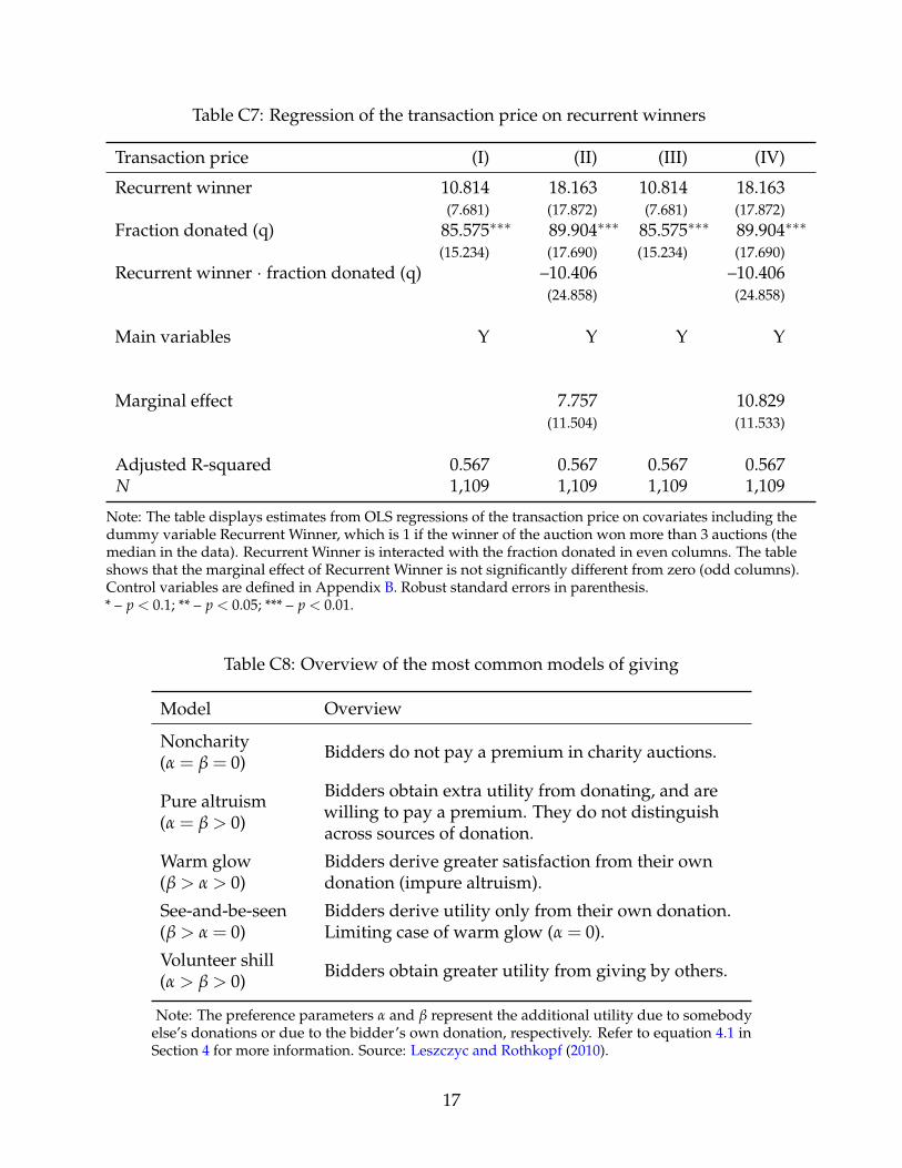
Table C7: Regression of the transaction price on recurrent winners

Transaction price (I) (II) (III) (IV)

Recurrent winner 10.814 18.163 10.814 18.163(7.681) (17.872) (7.681) (17.872)

Fraction donated (q) 85.575∗∗∗ 89.904∗∗∗ 85.575∗∗∗ 89.904∗∗∗

(15.234) (17.690) (15.234) (17.690)Recurrent winner · fraction donated (q) –10.406 –10.406

(24.858) (24.858)

Main variables Y Y Y Y

Marginal effect 7.757 10.829(11.504) (11.533)

Adjusted R-squared 0.567 0.567 0.567 0.567N 1,109 1,109 1,109 1,109

Note: The table displays estimates from OLS regressions of the transaction price on covariates including thedummy variable Recurrent Winner, which is 1 if the winner of the auction won more than 3 auctions (themedian in the data). Recurrent Winner is interacted with the fraction donated in even columns. The tableshows that the marginal effect of Recurrent Winner is not significantly different from zero (odd columns).Control variables are defined in Appendix B. Robust standard errors in parenthesis.* – p < 0.1; ** – p < 0.05; *** – p < 0.01.

Table C8: Overview of the most common models of giving

Model Overview

Noncharity(α = β = 0) Bidders do not pay a premium in charity auctions.

Pure altruism(α = β > 0)

Bidders obtain extra utility from donating, and arewilling to pay a premium. They do not distinguishacross sources of donation.

Warm glow(β > α > 0)

Bidders derive greater satisfaction from their owndonation (impure altruism).

See-and-be-seen(β > α = 0)

Bidders derive utility only from their own donation.Limiting case of warm glow (α = 0).

Volunteer shill(α > β > 0) Bidders obtain greater utility from giving by others.

Note: The preference parameters α and β represent the additional utility due to somebodyelse’s donations or due to the bidder’s own donation, respectively. Refer to equation 4.1 inSection 4 for more information. Source: Leszczyc and Rothkopf (2010).

17

Table C9: First step of the structural estimation

(I) (II)log(Transaction price) Coefficient S.E.

log(Reserve price) 0.371∗∗∗ (0.024)Minimum increment 0.019 (0.014)Minimum increment2 0.0001 (0.0004)log(Number of bidders) 0.036 (0.044)Sold at reserve price (0/1) −0.121∗∗ (0.049)log(Total number of bids placed) 0.261∗∗∗ (0.028)Length 0.052∗∗∗ (0.018)Length2 −0.002∗∗∗ (0.001)Extended time (0/1) −0.029 (0.030)Length of description 0.001∗∗ (0.0004)Content in English −0.057 (0.037)Content in Spanish −0.010 (0.138)Length of charity description −0.0003 (0.0003)Number of pictures −0.029 (0.022)Number of pictures2 0.003 (0.002)Number of same team auctions within 3 weeks 0.010∗∗ (0.004)Number of same player auctions within 2 weeks 0.009∗∗∗ (0.002)Number auctions from the same charity −0.001∗∗∗ (0.0002)Player belongs to FIFA 100 list (0/1) 0.110∗∗ (0.047)Unwashed jersey (0/1) 0.207∗∗∗ (0.048)Jersey is signed (0/1) 0.086∗∗ (0.037)Jersey is signed by the team players/coach (0/1) 0.061 (0.074)Jersey worn during a final (0/1) 0.338∗∗∗ (0.098)Number of goals scored wearing the jersey 0.186∗∗∗ (0.061)Player belongs to an important team (0/1) 0.242∗∗∗ (0.046)Charity is English (0/1) 0.168 (0.132)Charity is Italian (0/1) 0.208 (0.134)Charity deals with disabilities (0/1) 0.088∗∗ (0.039)Charity builds infrastructures in developing countries (0/1) 0.153∗∗ (0.069)Charity deals in healthcare (0/1) −0.146∗∗ (0.057)Charity has a humanitarian scopes in developing countries (0/1) 0.094 (0.065)Charity deals with children’s wellbeing (0/1) 0.068 (0.064)Charity deals with neurodgenerative disorders (0/1) 0.041 (0.084)Charity belongs to a soccer team (0/1) −0.185∗∗ (0.081)Charity aims to improve access to sport (0/1) 0.010 (0.066)Constant 2.225∗∗∗ (0.249)

Adjusted R-squared 0.522F Statistic 23.708∗∗∗ (df = 35; 694)N 730

Note:The table displays estimates from OLS regressions of the logarithm of the transaction price as in thefirst step of the structural model. (0/1) indicates dummies. Control variables are defined in Appendix B.Robust standard errors in parenthesis in column 2.* – p < 0.1; ** – p < 0.05; *** – p < 0.01.

18

Table C10: Estimated altruistic demand parameters with instruments

Number of bidders α βQuantile n [95% CI] [95% CI]

99% 16 17.3% 43.1%[6.12%, 29.6%] [18.5% 63.4%]

95% 14 17.1% 43.0%[8.1%, 30.6%] [21.9% 63.9%]

90% 12 16.8% 43.0%[7.4%, 28.9%] [23.6% 60.7%]

75% 10 16.4% 42.9%[7.3%, 28.5%] [22.2% 60.9%]

50% 7 15.4% 42.8%[7.3%, 25.4%] [24.3% 60.3%]

Note: The table displays results from the structural estimation of α and β for selected quantiles of thedistribution of the number of bidders. The first step regression is replaced with a 2SLS regression, wherethe reserve price is instrumented with the average reserve price and the average number of bids placed inconcurrent auctions (±5 days). The F-test is 33.269, and the over-identification test statistics (Sargan test) hasa p-value of 0.192. The preference parameters α and β represent the additional utility due to somebody else’sdonations or due to the bidder’s own donation, respectively. Refer to equation 4.1 in Section 4 for moreinformation. The 95% confidence intervals are reported in square brackets. The CI are found by bootstrapwith replacement (401 times). Dataset restricted to all auctions such that q ∈ {10%,85%}. 727 observations intotal.

Table C11: The impact of the fraction donated on the number of auctions over time

Number of auctions (weekly) (I) (II) (III)

Lagged number of auctions (weekly) 0.003 0.002 0.003(0.068) (0.068) (0.068)

Average q (weekly) –5.282 –5.183 –5.544(5.609) (5.713) (5.854)

Average q (weekly) , lag 1 week –0.526 –0.816(4.980) (5.181)

Average q (weekly) , lag 2 week 1.965(4.960)

Adjusted R-squared 0.302 0.299 0.293N 266 266 265

Note: The table displays estimates from OLS regressions of the weekly number of auctions. The data includesall auctions of actually worn soccer jerseys between June 19th, 2013, and November 6th, 2018 (3,968 auctions,267 weeks in total). All regressions include a constant and month and year fixed effects. The qualitativeresults would not change using monthly data. Robust standard errors in parentheses.* – p < 0.1; ** – p < 0.05; *** – p < 0.01.

19

Table C12: The impact of the fraction donated on the number of bidders over time

Independent Variables

Lagged Avg. q Avg. q Avg. q Adj. NDep. Var. (week) (lag 1) (lag 2) R-sq.

Dependent variable: Average number of bidders (weekly)Average num. bidders 0.289∗∗ 1.380 0.559 266

(0.866) (0.850)Average num. bidders 0.282∗∗∗ 1.198 1.048 0.560 266

(0.055) (0.864) (0.759)Average num. bidders 0.288∗∗∗ 1.306 1.136 –0.683 0.554 265

(0.055) (0.863) (0.771) (0.769)

Dependent variable: Median number of bidders (weekly)Q(50%) num. bidders 0.346∗∗∗ 1.438 0.492 266

(0.062) (0.940)Q(50%) num. bidders 0.342∗∗∗ 1.334 0.596 0.491 266

(0.061) (0.970) (0.861)Q(50%) num. bidders 0.350∗∗∗ 1.497 0.729 –1.005 0.486 265

(0.062) (0.955) (0.865) (0.850)

Dependent variable: 8th decile of the number of bidders (weekly)Q(80%) num. bidders 0.228∗∗∗ 1.045 0.520 266

(0.059) (1.154)Q(80%) num. bidders 0.224∗∗∗ 0.721 1.761∗ 0.522 266

(0.059) (1.150) (1.045)Q(80%) num. bidders 0.228∗∗∗ 0.652 1.712 0.268 0.514 265

(0.059) (1.172) (1.059) (1.111)

Note: The table displays estimates from OLS regressions of the weekly number of bidders. The dependentvariable varies across rows, while the independent variables vary across columns. The lagged dependentvariable is in column 1. Weekly observations. The data includes all auctions of actually worn soccer jerseysbetween June 19th, 2013, and November 6th, 2018 (3,968 auctions, 267 weeks in total). All regressions includea constant and month and year fixed effects. The qualitative results would not change using monthly data.Robust standard errors in parentheses.* – p < 0.1; ** – p < 0.05; *** – p < 0.01.

20

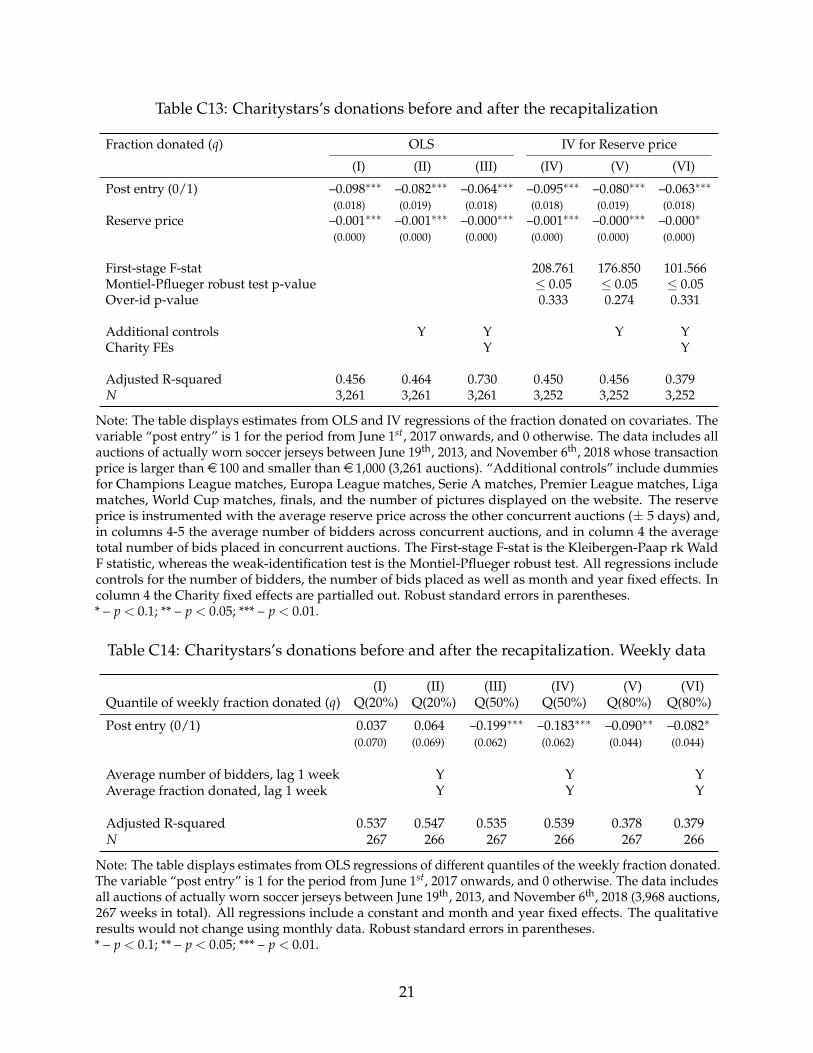
Table C13: Charitystars’s donations before and after the recapitalization

Fraction donated (q) OLS IV for Reserve price

(I) (II) (III) (IV) (V) (VI)

Post entry (0/1) –0.098∗∗∗ –0.082∗∗∗ –0.064∗∗∗ –0.095∗∗∗ –0.080∗∗∗ –0.063∗∗∗

(0.018) (0.019) (0.018) (0.018) (0.019) (0.018)Reserve price –0.001∗∗∗ –0.001∗∗∗ –0.000∗∗∗ –0.001∗∗∗ –0.000∗∗∗ –0.000∗

(0.000) (0.000) (0.000) (0.000) (0.000) (0.000)

First-stage F-stat 208.761 176.850 101.566Montiel-Pflueger robust test p-value ≤ 0.05 ≤ 0.05 ≤ 0.05Over-id p-value 0.333 0.274 0.331

Additional controls Y Y Y YCharity FEs Y Y

Adjusted R-squared 0.456 0.464 0.730 0.450 0.456 0.379N 3,261 3,261 3,261 3,252 3,252 3,252

Note: The table displays estimates from OLS and IV regressions of the fraction donated on covariates. Thevariable “post entry” is 1 for the period from June 1st, 2017 onwards, and 0 otherwise. The data includes allauctions of actually worn soccer jerseys between June 19th, 2013, and November 6th, 2018 whose transactionprice is larger than e 100 and smaller than e 1,000 (3,261 auctions). “Additional controls” include dummiesfor Champions League matches, Europa League matches, Serie A matches, Premier League matches, Ligamatches, World Cup matches, finals, and the number of pictures displayed on the website. The reserveprice is instrumented with the average reserve price across the other concurrent auctions (± 5 days) and,in columns 4-5 the average number of bidders across concurrent auctions, and in column 4 the averagetotal number of bids placed in concurrent auctions. The First-stage F-stat is the Kleibergen-Paap rk WaldF statistic, whereas the weak-identification test is the Montiel-Pflueger robust test. All regressions includecontrols for the number of bidders, the number of bids placed as well as month and year fixed effects. Incolumn 4 the Charity fixed effects are partialled out. Robust standard errors in parentheses.* – p < 0.1; ** – p < 0.05; *** – p < 0.01.

Table C14: Charitystars’s donations before and after the recapitalization. Weekly data

(I) (II) (III) (IV) (V) (VI)Quantile of weekly fraction donated (q) Q(20%) Q(20%) Q(50%) Q(50%) Q(80%) Q(80%)

Post entry (0/1) 0.037 0.064 –0.199∗∗∗ –0.183∗∗∗ –0.090∗∗ –0.082∗

(0.070) (0.069) (0.062) (0.062) (0.044) (0.044)

Average number of bidders, lag 1 week Y Y YAverage fraction donated, lag 1 week Y Y Y

Adjusted R-squared 0.537 0.547 0.535 0.539 0.378 0.379N 267 266 267 266 267 266

Note: The table displays estimates from OLS regressions of different quantiles of the weekly fraction donated.The variable “post entry” is 1 for the period from June 1st, 2017 onwards, and 0 otherwise. The data includesall auctions of actually worn soccer jerseys between June 19th, 2013, and November 6th, 2018 (3,968 auctions,267 weeks in total). All regressions include a constant and month and year fixed effects. The qualitativeresults would not change using monthly data. Robust standard errors in parentheses.* – p < 0.1; ** – p < 0.05; *** – p < 0.01.

21

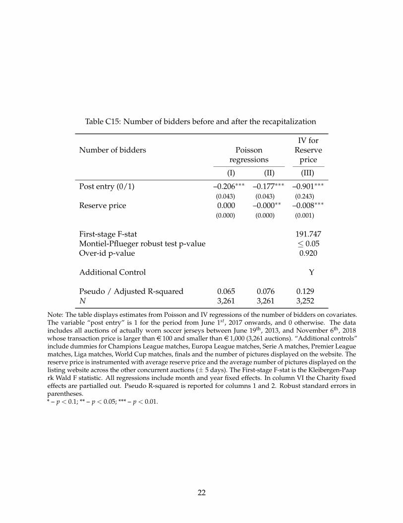
Table C15: Number of bidders before and after the recapitalization

IV forNumber of bidders Poisson Reserve

regressions price

(I) (II) (III)

Post entry (0/1) –0.206∗∗∗ –0.177∗∗∗ –0.901∗∗∗

(0.043) (0.043) (0.243)Reserve price 0.000 –0.000∗∗ –0.008∗∗∗

(0.000) (0.000) (0.001)

First-stage F-stat 191.747Montiel-Pflueger robust test p-value ≤ 0.05Over-id p-value 0.920

Additional Control Y

Pseudo / Adjusted R-squared 0.065 0.076 0.129N 3,261 3,261 3,252

Note: The table displays estimates from Poisson and IV regressions of the number of bidders on covariates.The variable “post entry” is 1 for the period from June 1st, 2017 onwards, and 0 otherwise. The dataincludes all auctions of actually worn soccer jerseys between June 19th, 2013, and November 6th, 2018whose transaction price is larger than e 100 and smaller than e 1,000 (3,261 auctions). “Additional controls”include dummies for Champions League matches, Europa League matches, Serie A matches, Premier Leaguematches, Liga matches, World Cup matches, finals and the number of pictures displayed on the website. Thereserve price is instrumented with average reserve price and the average number of pictures displayed on thelisting website across the other concurrent auctions (± 5 days). The First-stage F-stat is the Kleibergen-Paaprk Wald F statistic. All regressions include month and year fixed effects. In column VI the Charity fixedeffects are partialled out. Pseudo R-squared is reported for columns 1 and 2. Robust standard errors inparentheses.* – p < 0.1; ** – p < 0.05; *** – p < 0.01.

22

D Additional Figures

Figure D1: The webpage of a listing at the time of data collection

Title

Charity

Pictures %donated

Countdown

Currentprice

Inforeserveprice

Auctionleader

Description

Note: Screenshot of a webpage of a running auction on Charitystars.com for an AC Milan jersey worn andsigned by the player Giacomo Bonaventura. The standing price is GBP 110: this bid was placed by an Italianbidder with username “Supermanfra”. A total of five bids are placed at this point. Although at the currenthighest bid the reserve price is not met, this can change by the end of the auction. The auction will be activefor other 3 days and 18 hours and will expire on June 7th at 7AM. 85% of the proceeds will be donated to“Play for Change”.

23

Figure D2: How the firm allocates the funds at the time of data collection

Note: Screenshot describing how the firm allocates the fraction donated at the time of scraping.

Figure D3: Plot of the coefficient for the fraction donated from a quantile regression

0.2 0.4 0.6 0.8

0.1

0.2

0.3

0.4

Quantile of log(Price)

Coeffic

ient of F

raction D

onate

d (

q)

Note: The plot displays coefficients from quantile regressions of the logarithm of the transaction price onq and covariates as in the first column of Table C1 in the main text. The shaded regions is the confidenceinterval. The dashed (dotted) line reports the coefficient of the OLS regression (5% confidence interval).Appendix Table C1 shows the coefficients for each quartile. Only auctions with price between e 100 ande 1000. Boostrapped standard errors with 400 repetitions.

24

Figure D4: Density of the homogenized transaction prices by returning winners vs non-returning winners

0.0

0.2

0.4

0.6

0.8

1.0

1.2

−1.2 −0.9 −0.6 −0.3 0 0.3 0.6 0.9 1.2 1.5Pseudo−winning bids

pdf

CollectorsOthers

Note: The plot display the density of the pseudo-winning bids from the first-step of the structural modeldistinguishing by returning winners. Returning winners (or collectors) are bidders who won at least 4auctions (the median is 3). The Kolmogorov-Smirnov test does not reject the null hypothesis that the twodensities are equal at 0.4097 level. The plot is obtained using only auctions with q ∈ {10%,85%}. The plotteddensities are computed using a Gaussian kernel and Silverman’s rule-of-thumb bandwidths (Silverman,1986).

Figure D5: Comparison between the model implied prices and observed average prices

(a) Deviation from average price (%)

−20

−10

0

10

20

5 6 7 8 9 10Number of Bidders

Devia

tion fro

m A

vera

ge P

rice (

%)

q=0.10 q=0.85

(b) Number of auctions per number of bidders

0

20

40

60

5 6 7 8 9 10Number of Bidders

Observ

ations

q=0.10 q=0.85

Note: Panel a. The barplot displays the percentage difference between the observed price in the data andthe expected price implied by the model for different number of bidders. A positive number indicates thatthe model overstates prices. Panel b. The barplot displays the number of auctions such that the number ofbidders joining the auction is equal to that indicated in the x axis.

25

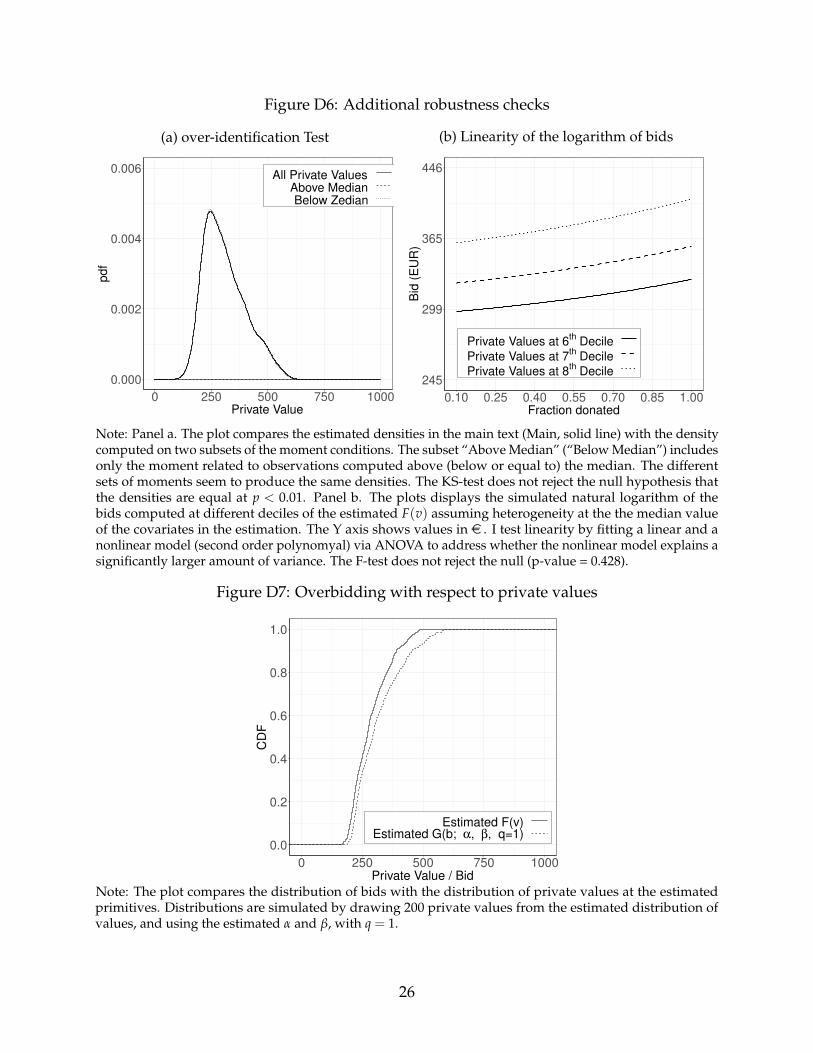
Figure D6: Additional robustness checks

(a) over-identification Test

0.000

0.002

0.004

0.006

0 250 500 750 1000Private Value

pdf

All Private ValuesAbove MedianBelow Zedian

(b) Linearity of the logarithm of bids

245

299

365

446

0.10 0.25 0.40 0.55 0.70 0.85 1.00Fraction donated

Bid

(E

UR

)

Private Values at 6th Decile

Private Values at 7th Decile

Private Values at 8th Decile

Note: Panel a. The plot compares the estimated densities in the main text (Main, solid line) with the densitycomputed on two subsets of the moment conditions. The subset “Above Median” (“Below Median”) includesonly the moment related to observations computed above (below or equal to) the median. The differentsets of moments seem to produce the same densities. The KS-test does not reject the null hypothesis thatthe densities are equal at p < 0.01. Panel b. The plots displays the simulated natural logarithm of thebids computed at different deciles of the estimated F(v) assuming heterogeneity at the the median valueof the covariates in the estimation. The Y axis shows values in e . I test linearity by fitting a linear and anonlinear model (second order polynomyal) via ANOVA to address whether the nonlinear model explains asignificantly larger amount of variance. The F-test does not reject the null (p-value = 0.428).

Figure D7: Overbidding with respect to private values

0.0

0.2

0.4

0.6

0.8

1.0

0 250 500 750 1000Private Value / Bid

CD

F

Estimated F(v)Estimated G(b; α, β, q=1)

Note: The plot compares the distribution of bids with the distribution of private values at the estimatedprimitives. Distributions are simulated by drawing 200 private values from the estimated distribution ofvalues, and using the estimated α and β, with q = 1.

26

E Robustness Checks for the Optimal Fraction DonatedI propose several robustness checks to the main text analysis. All estimates report robust standarderrors. Confidence intervals for the optimal q are obtained through 401 bootstrap replications ofthe estimation algorithm with replacement.

Optimal Fraction Donated with More Covariates. I include all the variables in the dataset as inthe fourth column of Table 1 by adding to the first-step regressions of both the demand and supplymodel the variables belonging to the groups “Additional Charity Dummies”, “League/MatchDummies” and “Time Dummies.” Figure E1 shows the optimal fraction donated by intersectingmarginal revenues and marginal costs as in Section 7. On the supply side the marginal costparameters are π1 = 229.275,SE : 11.822;π2 = −400.940;SE : 55.084;π3 = 187.354,SE : 53.151, whileon the demand side α is estimated to be 0.172 and β is 0.431 when the number of bidders is 16. Theoptimal fraction donated is q∗ = 0.20 (95% C.I. [0.025,0.475]).

Optimal q∗ by Type of Provider. I further investigate whether the optimal fraction donated variesconsistently based on the type of provider. When available, I observe whether the object is providedby either a footballer, a coach or a charity (672 auctions). Because footballers and coaches are closelytied to certain charities, I separate the auctions in the sample in two based on whether the providerof the auctioned item is a private individual or not, and estimate marginal costs on each subsamplein the same way as in Section 7.

The marginal cost for the whole group including footballers and charities are negative andupward sloping (π1 = 248.388,SE : 28.495;π2 = −557.406;SE : 54.894;π3 = 349.055,SE : 56.898).Figure E2 plots the optimal q obtained for this group. I find that q∗ = 0.32 (95% C.I. [0.045,0.420]),which is very close to that estimated in the full sample (see Figure 5a). The qualitative result doesnot change if I replicate the analysis to account for the auctions provided by charities (469 auctions,π1 = 259.095,SE : 42.792;π2 = −677.876;SE : 321.572;π3 = 478.420,SE : 323.874). In this case, q∗ is0.36 (95% C.I. [0.045,0.435]).

Optimal q∗ Using IVs. As the reserve price and the fraction donated are the result of bargainingbetween the provider of the item and Charitystars, in this section, I instrument the reserve price inthe demand model and the fraction donated in the supply model. On the demand side, I performa two-stage least square regression in place of equation 6.1; I instrument the reserve price withthe average reserve price (in logs) and the average number of bids placed in concurrent auctions(within 5 days). The estimated α and β are 0.173 and 0.431. The F-test is large 33.269, and theover-identification test statistic has a p-value of 0.192 (Sargan test).

On the supply side, I follow the same steps in Section 7. In the last step, instead of performingan OLS regression of the net reserve price on a polynomial expansion of q, I instrument q and q2

with the average fraction donated (and its squared value) and the average number of bids placed(and its squared value) across concurrent auctions (within 5 days). The estimated marginal costparameters are π1 = 273.389,SE : 44.128;π2 = −650.978;SE : 298.535;π3 = 422.534,SE : 296.863.The F-test for the first endogenous regressor (q) is 30.637 and for the second endogenous regressor(q2) is 33.063. The over-identification test has a p-value of 0.907. Despite the strong first stages, theinstruments would fail if the choice of the fraction donated and of the reserve price systematicallyresponded to common shocks across concurrent auctions. I include the number of listings of jerseysfrom the same team in the previous 3 weeks and for the same player in the previous 2 weeks amongthe covariates to control for this issue.

Figure E3 plots both the marginal revenue and marginal cost curves (Panel a) and the expectedprofits attainable at different fraction donated (Panel b). Both plots indicate that the optimal fraction

27

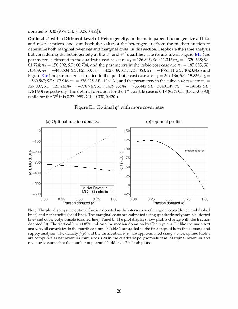
donated is 0.30 (95% C.I. [0.025,0.455]).

Optimal q∗ with a Different Level of Heterogeneity. In the main paper, I homogeneize all bidsand reserve prices, and sum back the value of the heterogeneity from the median auction todetermine both marginal revenues and marginal costs. In this section, I replicate the same analysisbut considering the heterogeneity at the 1st and 3rd quartiles. The results are in Figure E4a (theparameters estimated in the quadratic-cost case are π1 = 176.845,SE : 11.346;π2 = −320.638;SE :61.724;π3 = 158.392,SE : 60.704, and the parameters in the cubic-cost case are π1 = 187.055,SE :70.489;π2 = −445.534;SE : 823.537;π3 = 432.089,SE : 1738.863,π4 = −166.111;SE : 1020.906) andFigure E4c (the parameters estimated in the quadratic-cost case are π1 = 309.186,SE : 19.836;π2 =−560.587;SE : 107.916;π3 = 276.925,SE : 106.131, and the parameters in the cubic-cost case are π1 =327.037,SE : 123.24;π2 = −778.947;SE : 1439.83;π3 = 755.442,SE : 3040.149,π4 = −290.42;SE :1784.90) respectively. The optimal donation for the 1st quartile case is 0.18 (95% C.I. [0.025,0.330])while for the 3rd it is 0.27 (95% C.I. [0.030,0.420]).

Figure E1: Optimal q∗ with more covariates

(a) Optimal fraction donated

−600

−500

−400

−300

−200

−100

0

0.00 0.25 0.50 0.75 1.00Fraction donated (q)

MR

, M

C (

EU

R)

M Net RevenueMC − Quadratic

(b) Optimal profits

median donation

−25

0

25

50

75

100

125

150

0.00 0.25 0.50 0.75 1.00Fraction donated (q)

Pro

fits

(E

UR

)

Note: The plot displays the optimal fraction donated as the intersection of marginal costs (dotted and dashedlines) and net benefits (solid line). The marginal costs are estimated using quadratic polynomials (dottedline) and cubic polynomials (dashed line). Panel b. The plot displays how profits change with the fractiondoanted (q). The vertical line at 85% indicate the median donation by Charitystars. Unlike the main textanalysis, all covariates in the fourth column of Table 1 are added to the first steps of both the demand andsupply analyses. The density f (v) and the distribution F(v) are approximated using a cubic spline. Profitsare computed as net revenues minus costs as in the quadratic polynomials case. Marginal revenues andrevenues assume that the number of potential bidders is 7 in both plots.

28

Figure E2: Optimal q∗ by type of provider

(a) Optimal fraction donated

−600

−500

−400

−300

−200

−100

0

0.00 0.25 0.50 0.75 1.00Fraction donated (q)

MR

, M

C (

EU

R)

M Net RevenueMC − Players, Charities

MC − Charities only

(b) By providers

median donation

−25

0

25

50

75

100

125

150

0.00 0.25 0.50 0.75 1.00Fraction donated (q)

Pro

fits

(E

UR

)

Note: The plot displays the optimal fraction donated as the intersection of marginal costs (dotted and dashedlines) and net benefits (solid line). The marginal costs are estimated using quadratic polynomials. Unlikethe main text analysis, I limit the dataset to auctions of item provided by either charities (dashed line) orfootballers and charities (dotted line). Panel b. The plot displays how profits change with the fractiondoanted (q). The vertical line at 85% indicate the median donation by Charitystars. The density f (v) and thedistribution F(v) are approximated using a cubic spline. Profits are computed as net revenues minus costsas in the quadratic polynomials case. Marginal revenues and revenues assume that the number of potentialbidders is 7 in both plots.

29

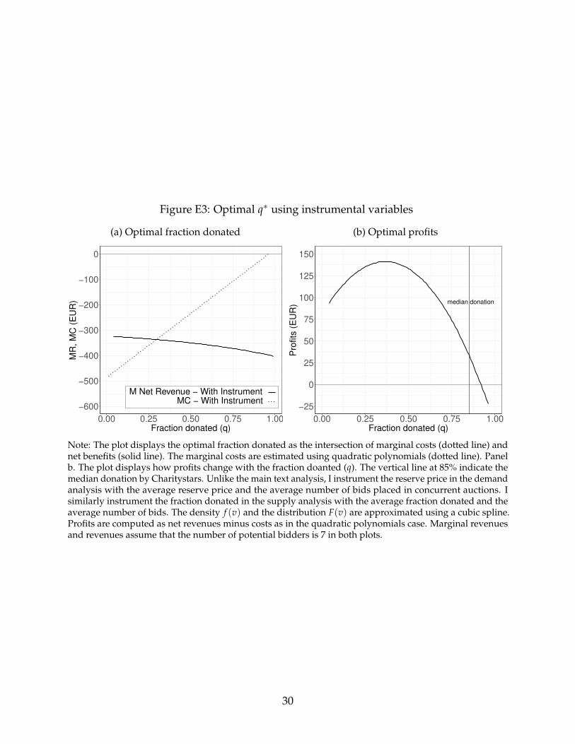
Figure E3: Optimal q∗ using instrumental variables

(a) Optimal fraction donated

−600

−500

−400

−300

−200

−100

0

0.00 0.25 0.50 0.75 1.00Fraction donated (q)

MR

, M

C (

EU

R)

M Net Revenue − With InstrumentMC − With Instrument

(b) Optimal profits

median donation

−25

0

25

50

75

100

125

150

0.00 0.25 0.50 0.75 1.00Fraction donated (q)

Pro

fits

(E

UR

)

Note: The plot displays the optimal fraction donated as the intersection of marginal costs (dotted line) andnet benefits (solid line). The marginal costs are estimated using quadratic polynomials (dotted line). Panelb. The plot displays how profits change with the fraction doanted (q). The vertical line at 85% indicate themedian donation by Charitystars. Unlike the main text analysis, I instrument the reserve price in the demandanalysis with the average reserve price and the average number of bids placed in concurrent auctions. Isimilarly instrument the fraction donated in the supply analysis with the average fraction donated and theaverage number of bids. The density f (v) and the distribution F(v) are approximated using a cubic spline.Profits are computed as net revenues minus costs as in the quadratic polynomials case. Marginal revenuesand revenues assume that the number of potential bidders is 7 in both plots.

30

Figure E4: Optimal q∗ with a different level of heterogeneity

(a) Optimal fraction donated (25-percentile)

−600

−500

−400

−300

−200

−100

0

0.00 0.25 0.50 0.75 1.00Fraction donated (q)

MR

, M

C (

EU

R)

M Net RevenueMC − Quadratic

MC − Cubic

(b) Optimal profits (25-percentile)

median donation

−25

0

25

50

75

100

125

150

0.00 0.25 0.50 0.75 1.00Fraction donated (q)

Pro

fits

(E

UR

)

(c) Optimal fraction donated (75-percentile)

−600

−500

−400

−300

−200

−100

0

0.00 0.25 0.50 0.75 1.00Fraction donated (q)

MR

, M

C (

EU

R)

M Net RevenueMC − Quadratic

MC − Cubic

(d) Optimal profits (75-percentile)

median donation

−25

0

25

50

75

100

125

150

0.00 0.25 0.50 0.75 1.00Fraction donated (q)

Pro

fits

(E

UR

)

The plot displays the optimal fraction donated as the intersection of marginal costs (dotted and dashed lines)and net benefits (solid line). The marginal costs are estimated using quadratic polynomials. Panel b. Theplot displays how profits change with the fraction doanted (q). The vertical line at 85% indicate the mediandonation by Charitystars. Unlike the main text analysis, I fit revenues and costs to represents either the 25th-or 75th- percentile of auction heterogeneity. The density f (v) and the distribution F(v) are approximatedusing a cubic spline. Profits are computed as net revenues minus costs as in the quadratic polynomials case.Marginal revenues and revenues assume that the number of potential bidders is 7 in all plots.

31

F Monte Carlo simulationsObjectives. The Monte Carlo simulations in this section fulfil two goals: (i) to show that theestimation routine described in Section 6 return consistent estimates of the parameters, and (ii) tosupport with some empirical evidence the claim that the estimates are not consistent when thefranction donated in the two auction types is very close.

Design of the experiments. There are two auction types (A and B) such that qA = .10 and qB = .85.Private values are generated for all bidders drawing from a uniform distribution in [0,1] in TablesF1 and F2 and in [−1,1] in Tables F3. There are 10 bidders in each auctions. They bid according tothe bid function in equation 4.2. The true charitable parameters are α0 = .25 and β0 = .75.

The steps of the estimation procedure are outlined below:

1. Draw values from the distribution F(v) for each bidder in the two auctions. In total 20 values.

2. Compute the bids for each bidder in the two auctions. Save the winning bid in each auction.

3. Nonparametrically estimate the density of the winning bids (either by Triweight, or GaussianKernel). The bandwidth is chosen using the rule-of-thumb. Trimming follows Guerre et al.(2000) who suggested trimming observations close to 0.5× bandwidth to the boundary.5

4. Given the number of bidders (n = 10) invert the distribution of the winning bids to determinethe distribution and density of the bids as in the second stage of the estimation procedure.

5. Compute the distribution and density of auctions of type A for each losing bids in the intervalbetween the smallest winning bid and the largest winning bid of type A.

6. Compute the distribution and density of type B (q = .85) over 100,000 points.

7. Match the quantile of the distribution of type B with those of the distribution of type Athrough equation 5.1.

8. Find the couple (α, β) that minimizes the objective function equation 6.2 starting from arandom seed. The search algorithm constraints the parameters in the unit interval.

9. Save the estimates and restart from 1.

These steps are repeated 401 times. The tables below report the mean, median, quantiles and rootmean squared errors for α and β for each combination of parameters.

Results. First, let’s asses the consistency of the estimates. Different experiments are reported inTables F2 and F3, showing that the estimates are close to the true parameters. In particular, evenwith a small number of observations (the first line in each panel), the mean and medians are alwayswithin 3% of the true parameters.

These tables are composed by different panels: each panel refers to a different kernel used toestimate the distributions (and densities) of the winning bids. The Gaussian and Triweigth kernelsgive similar results. Within each panel, the rows differ on the number of auctions used to estimatethe primitives. The number of bidders in each auction is always constant and equal to 10. Since

5For the Gaussian case the hpd f = 1.06σn−1/5 and hCDF = 1.06σn−1/3 where σ =

min{s.d.(bkw), IQR/1.349}, where bk

w is the vector of winning bid for auction of type k, andhCDF = 1.587σn−1/3. For the triweight case hpd f = hCDF = 2.978σn−1/5 (Hardle, 1991, Li et al.,2002, Li and Racine, 2007, Lu and Perrigne, 2008).

32

for each auction only the winning bid is used, I empirically consider the asymptotic properties ofthe estimator by looking at the rate at which the root mean squared error (RMSE) decreases as thenumber of auctions grows (i.e., comparing RMSE across columns).6 Comfortingly, this rate is closeto√

n for all experiments.To study the consistency of the estimates when there is only limited variation over q across

auctions I run similar experiments varying q instead of the nonparametric kernel. From Table F1 itis clear that α and β cannot be estimated consistently when qA ' qB as the mean and median of theestimated parameters are about 0 and .50 instead of .25 and .75 for α and β respectively.

Table F1: Distance between qA and qB – Monte Carlo simulations

TA TB µα µβ Medα Medβ 25%α 75%α 25%β 25%β

qA = 80%, qB = 85%500 0.0069 0.5333 0.0000 0.5328 0.0000 0.0000 0.5053 0.55891000 0.0094 0.5355 0.0000 0.5302 0.0000 0.0078 0.5114 0.5560

qA = 78%, qB = 85%500 0.0158 0.5414 0.0000 0.5350 0.0000 0.0151 0.5137 0.56061000 0.0227 0.5477 0.0028 0.5376 0.0000 0.0348 0.5181 0.5667

qA = 50%, qB = 85%500 0.2027 0.7086 0.1914 0.6991 0.1360 0.2520 0.6455 0.75791000 0.2154 0.7196 0.2071 0.7132 0.1696 0.2636 0.6763 0.7620

qA = 20%, qB = 85%500 0.2468 0.7467 0.2383 0.7398 0.1984 0.2891 0.7033 0.78521000 0.2462 0.7463 0.2445 0.7444 0.2166 0.2764 0.7186 0.7730

Note: Monte Carlo simulations of the second and third step of the estimation process. Auction types aredenoted by A and B. Each panel shows the estimated parameters for different percentage donated. Thebandwidths in step 2 are computed with a Gaussian Kernel. The data is generated according to α = 25%,β = 75% and F(v) is assumed uniform in [0,1]. Each auction has 10 bidders. 401 repetitions.

6I am analyzing the asymptotic properties of this class of estimators theoretically in another project, whichis still a work in progress.

33

Tabl

eF2

:Mon

teC

arlo

sim

ulat

ion

1

TA

TB

µα

µβ

Med

αM

edβ

25%

α75

%α

25%

β25

%β

10%

α90

%α

10%

β90

%β

RM

SEα

RM

SEβ

Gau

ssia

nke

rnel

3411

20.

2760

0.77

230.

2681

0.77

060.

1513

0.42

020.

6577

0.89

630.

0631

0.49

540.

5846

0.99

000.

1587

0.14

6917

256

00.

2682

0.76

580.

2647

0.76

270.

2160

0.31

950.

7176

0.81

360.

1725

0.36

990.

6781

0.85

830.

0789

0.07

2610

00.

2637

0.76

150.

2449

0.74

420.

1759

0.35

060.

6802

0.83

680.

1148

0.44

590.

6234

0.93

450.

1225

0.11

3550

00.

2507

0.75

000.

2428

0.74

520.

2089

0.29

140.

7122

0.78

550.

1813

0.32

580.

6881

0.81

900.

0586

0.05

3410

000.

2498

0.74

940.

2475

0.74

700.

2227

0.27

640.

7253

0.77

260.

1965

0.30

560.

7010

0.80

200.

0412

0.03

77

Triw

eigt

hke

rnel

3411

20.

2318

0.73

910.

2051

0.71

360.

1172

0.35

000.

6281

0.84

790.

0460

0.47

250.

5644

0.98

480.

1522

0.14

5317

256

00.

2310

0.73

460.

2267

0.73

090.

1797

0.28

020.

6875

0.78

200.

1347

0.33

230.

6421

0.82

770.

0767

0.07

1810

00.

2855

0.78

370.

2820

0.77

970.

1953

0.37

420.

6990

0.86

010.

1172

0.48

530.

6293

0.98

060.

1314

0.12

3850

00.

2547

0.75

430.

2535

0.75

220.

2115

0.29

100.

7145

0.78

950.

1855

0.33

040.

6866

0.82

540.

0579

0.05

3610

000.

2503

0.75

070.

2507

0.75

030.

2209

0.27

650.

7233

0.77

630.

1998

0.30

310.

7054

0.79

960.

0412

0.03

78

Not

e:M

onte

Car

losi

mul

atio

nsof

the

seco

ndan

dth

ird

step

ofth

ees

timat

ion

proc

ess.

Auc

tion

type

sar

ede

note

dby

Aan

dB

.The

band

wid

ths

inst

ep2

are

com

pu

ted

eith

erw

ith

aG

auss

ian

Ker

nel(

top

pan

el)o

rw

ith

aTr

iwei

gth

kern

el(b

otto

mp

anel

).T

hed

ata

isge

nera

ted

acco

rdin

gto

α=

25%

,β=

75%

,qA=

10%

,qB=

85%

and

F(v)

isas

sum

edun

ifor

min

[0,1].

Each

auct

ion

has

10bi

dder

s.40

1re

peti

tion

s.

Tabl

eF3

:Mon

teC

arlo

sim

ulat

ion

2

TA

TB

µα

µβ

Med

αM

edβ

25%

α75

%α

25%

β25

%β

10%

α90

%α

10%

β90

%β

RM

SEα

RM

SEβ

Gau

ssia

nke

rnel

3411

20.

2785

0.76

870.

2716

0.76

390.

1557

0.40

260.

6717

0.87

790.

0812

0.49

610.

6013

0.97

900.

1580

0.13

5017

256

00.

2661

0.76

110.

2636

0.75

920.

2169

0.31

280.

7194

0.80

480.

1763

0.35

880.

6851

0.84

100.

0735

0.06

2750

00.

2513

0.74

920.

2472

0.74

770.

2131

0.28

710.

7191

0.77

770.

1887

0.32

030.

6949

0.80

640.

0537

0.04

4910

000.

2506

0.74

910.

2480

0.74

690.

2255

0.27

550.

7282

0.77

050.

2023

0.30

350.

7080

0.79

190.

0380

0.03

19

Triw

eigt

hke

rnel

3411

20.

2342

0.75

860.

2166

0.74

500.

1206

0.35

010.

6429

0.87

870.

0543

0.43

880.

5805

0.99

000.

1416

0.14

7317

20.

2341

0.23

410.

7499

0.23

230.

7481

0.17

770.

2820

0.69

680.

7998

0.14

220.

3304

0.65

880.

8457

0.07

530.

0722

500

0.26

730.

7659

0.26

320.

7636

0.22

620.

3055

0.72

890.

8038

0.19

520.

3457

0.69

760.

8355

0.05

910.

0549

1000

0.25

830.

7587

0.25

780.

7589

0.23

050.

2838

0.73

490.

7827

0.21

030.

3110

0.71

270.

8025

0.04

030.

0364

Not

e:M

onte

Car

losi

mul

atio

nsof

the

seco

ndan

dth

ird

step

ofth

ees

timat

ion

proc

ess.

Auc

tion

type

sar

ede

note

dby

Aan

dB

.The

band

wid

ths

inst

ep2

are

com

pu

ted

eith

erw

ith

aG

auss

ian

Ker

nel(

top

pan

el)o

rw

ith

aTr

iwei

gth

kern

el(b

otto

mp

anel

).T

hed

ata

isge

nera

ted

acco

rdin

gto

α=

25%

,β=

75%

,qA=

10%

,qB=

85%

and

F(v)

isas

sum

edun

ifor

min

[−1,

1].E

ach

auct

ion

has

10bi

dder

s.40

1re

peti

tion

s.

34

References in the Online AppendixGUERRE, E., PERRIGNE, I. and VUONG, Q. (2000). Optimal nonparametric estimation of first-price

auctions. Econometrica: Journal of the Econometric Society, 68 (3), 525–574.

HARDLE, W. (1991). Smoothing techniques: with implementation in S. Springer Science & BusinessMedia.

LI, Q. and RACINE, J. S. (2007). Nonparametric econometrics: theory and practice. Princeton UniversityPress.

LI, T., PERRIGNE, I. and VUONG, Q. (2002). Structural estimation of the affiliated private valueauction model. RAND Journal of Economics, pp. 171–193.

LU, J. and PERRIGNE, I. (2008). Estimating risk aversion from ascending and sealed-bid auctions:the case of timber auction data. Journal of Applied Econometrics, 23 (7), 871–896.

35