stanford econ 266: international trade lecture 10...

Stanford Econ 266: International Trade— Lecture 10: Heckscher-Ohlin Empirics (I) —

Stanford Econ 266 (Dave Donaldson)

Winter 2015 (Lecture 10)

Stanford Econ 266 (Dave Donaldson) RV and HO Empirics (I) Winter 2015 (Lecture 10) 1 / 64

Plan of Today’s Lecture

1 Empirical work on Ricardo-Viner model:1 Introduction2 ‘Geographic Incidence’ approaches:

1 Topalova (2009)2 Kovak (2013)3 Dix-Carneiro (2014)4 Dix-Carneiro and Kovak (2014)

3 Areas for future research2 Empirical work on Heckscher-Ohlin model (part I):

1 Introduction2 Tests concerning the ‘goods content’ of trade

3 Appendix: More on the Ricardo-Viner model (for reading at home)1 Factor price responses to goods price changes:

1 Stock market event study approach: Grossman and Levinsohn (1987)2 Political economy approaches: Magee (1980), Mayda and Rodrik

(2005)

2 GNP function approach:1 Kohli (1993)









(2005)



Empirical Work on the Ricardo-Viner Model

Very little empirical work on the RV model. Why?

RV model is best thought of as the short- to medium-run of the H-Omodel so you’d expect an integrated, dynamic empirical treatment ofthe two models. However, most H-O empirics has traditionally beendone using a cross-section, which is usually thought of as a set ofcountries in long-run equilibrium. Hence, there was never a pressingneed to think about adjustment dynamics (i.e. the RV model).

There is probably also a sense that a serious treatment of thesedynamics is too complicated for aggregate data (even when aggregatepanel data are available).

The heightened availability of firm-level panel data opens up newpossibilities.

We will look here at papers that have identified and tested aspects ofRV model that are unique to RV model (at least relative to H-O).









(2005)



‘Regional Incidence’ of Trade Shocks

Suppose a change in trade policy affects p (one nation-wide goodsprice vector). How does this affect welfare (ie, real income, here) indifferent regions of a country?

This has been an important topic in the field of ‘Trade andDevelopment’.

This is the question that Topalova (AEJ Applied, 2009) and Kovak(AER 2013) propose, with respect to India and Brazil, respectively.

Porto (JIE, 2005), among others, also looks at this question.

And note that if one region were thought to be totally unaffected (e.g.a pure ‘control’ group) then this regional incidence method also allowsus to identify the aggregate effect of the shock.

The RV model (often implicitly) has been an influential theoreticalapproach within which to attack this empirical question.

Topalova (2009): labor is intersectorally immobile and geographicallyimmobileKovak (2013): labor is intersectorally immobile but geographicallymobile


Topalova (2009)

In an innovative paper, Topalova (2009) estimates the followingregression on Indian districts:

ydt = αd + βt + γTariffdt + εdt

Here, y is the poverty rate, and Tariffdt is calculated as the districtemployment-weighted average of national industry-wise tariffs.

India is attractive here for many reasons:India went through an important and controversial trade liberalizationin 1991 (and later in the 1990s).There are very good, long-running surveys of poverty, for which themicro data is available from (roughly) 1983 onwards.There are 400-600 districts, depending on the time period.

Topalova (2009) uses a (now standard) IV for tariffs:In trade liberalization episodes, higher tariffs have ‘further to fall’.So a plausible instrument for tariff changes is pre-liberalization tarifflevels.


Topalova (2009): Identification Strategy for Tariff Changes

Figure 1. Evolution of Tariffs in India

Panel G: Correlation of Industry Tariffs in 1997 and 1987 Panel H: Tariff Decline and Industry Tariffs in 1987

Panel A: Average Nominal Tariffs

0

20

40

60

80

100

120

1987 1988 1989 1990 1991 1992 1993 1994 1995 1996 1997 1998 1999 2000 2001

Panel B: Standard Deviation of Nominal Tariffs

0

10

20

30

40

50

60

1987 1988 1989 1990 1991 1992 1993 1994 1995 1996 1997 1998 1999 2000 2001

Panel C: Tariffs by Broad Industrial Category

0

20

40

60

80

100

120

1987

1989

1991

1993

1995

1997

1999

2001

Cereals andOilseedsAgriculture

Mining & Mfg-K

Mining & Mfg-C

Panel D: Tariffs by Industrial Use Based Category

0

20

40

60

80

100

120

1987

1989

1991

1993

1995

1997

1999

2001

Basic

Capital

ConsumerDurablesConsumer NonDurablesIntermediate

Panel E: Share of Free HS Lines by Broad Industrial Category

0

0.2

0.4

0.6

0.8

1

1.2

1989 1996 1998 2001

Cereals & OilseedsAgricultureMining & Mfg-KMining & Mfg-C

Panel F: Share of Free HS Lines by Industrial Use Based Category

0

0.2

0.4

0.6

0.8

1

1.2

1989 1996 1998 2001

Basic

Capital

Consumer Durables

Consumer NonDurablesIntermediate

050

100

150

200

1997

tarif

f

0 50 100 150 200 2501987 tariff

-50

050

100

150

200

chan

ge

0 50 100 150 200 2501987 tariff


Topalova (2009): Results

Tariff TrTariffIV-

TrTariffIV-TrTariff, Init TrTariff Tariff TrTariff

IV-TrTariff

IV-TrTariff, Init TrTariff

(1) (2) (3) (4) (5) (6) (7) (8)

Tariff Measure -0.287 ** -0.297 *** -0.834 *** -0.687 *** -0.215 -0.065 -0.156 -0.403(0.118) (0.084) (0.250) (0.225) (0.190) (0.156) (0.353) (0.275)

Obs 725 725 725 725 703 703 703 703

Tariff Measure -0.129 *** -0.114 *** -0.319 *** -0.206 *** -0.084 -0.032 -0.076 -0.131(0.038) (0.021) (0.073) (0.075) (0.052) (0.046) (0.101) (0.087)

Obs 725 725 725 725 703 703 703 703

Tariff Measure -0.086 -0.094 -0.265 -0.161 0.092 0.108 0.257 0.213(0.154) (0.082) (0.228) (0.183) (0.094) (0.115) (0.295) (0.250)

Obs 725 725 725 725 703 703 703 703

Tariff Measure -0.016 -0.020 -0.057 -0.020 0.034 0.090 0.215 0.172(0.066) (0.042) (0.115) (0.071) (0.062) (0.066) (0.174) (0.144)

Obs 725 725 725 725 703 703 703 703

Logmean -0.015 0.132 0.370 0.552 -0.063 -0.126 -0.301 0.048(0.314) (0.183) (0.522) (0.433) (0.150) (0.212) (0.521) (0.468)

Obs 725 725 725 725 703 703 703 703

Panel A. Dependent variable: Poverty Rate

Table 4a. Effect of Trade Liberalization on Poverty and Inequality in Indian Districts

I. RURAL II. URBAN

Note: All regressions include year and district dummies. Standard errors (in parentheses) are corrected for clustering at the state year level. Regressions are weighted by the square root of the number of people in a district. Significance at the 10 percent level of confidence is represented by a *, at the 5 percent level by **, and at the 1 percent level by ***.

Panel D. Dependent variable: Log Deviation of Consumption

Panel C. Dependent variable: StdLog Consumption

Panel B. Dependent variable: Poverty Gap

Panel E. Dependent variable: Log Average Per Capita Expenditures


Kovak (2013)

Kovak (2013) performs a similar exercise to Topalova (2009), butwith some attractive extensions:

The estimating equation emerges directly from a RV model.

The estimating equation is similar to Topalova (2009), but with aslight alteration to the way that Tariffdt is calculated (he uses differentweights and different treatment of the non-traded sector).

Unlike Topalova (2009), Kovak (2013) finds economically andstatistically significant migration responses: people appear to movearound the country in response to (national) tariff changes, to getcloser to favored industry-specific factors like capital/land.


Kovak (2013): Model

Consider general RV model, but with multiple regions r . For nowconsider one region.

Many industries i . Each with specific factor Ki . One factor L that ismobile across sectors (and in principle across regions).

Factor market clearing then requires (where afi is amount of factor frequired to produce in industry i):

aKiYi = Ki (1)∑i

aLiYi = L (2)

Differentiating this yields∑

i λi (aLi − aKi ) = L where λi ≡ LiL

Perfect competition requires aLiw + aKi ri = pi . Differentiating thatgives (1− θi )w + θi ri = pi (for all i), where θi ≡ ri Ki

pi Yi.


Kovak (2013): Model

Letting σi be the elasticity of substitution between Ki and L inindustry i we have (by definition):

aKi − aLi = σi (w − ri ) (3)

So combining the previous expressions we have∑i

λiσi (ri − w) = L (4)

This can be re-written as:

w =−L∑

i ′ λi ′σi′θi′

+∑

i

βi pi (5)

With βi ≡λi

σiθi∑

i′ λi′σi′θi′


Kovak (2013): Model

Letting σi be the elasticity of substitution between Ki and L inindustry i we have (by definition):

aKi − aLi = σi (w − ri ) (6)

So combining the previous expressions we have∑i

λiσi (ri − w) = L (7)


w =−L∑

i ′ λi ′σi′θi′

+∑

i

βi pi (8)

With βi ≡λi

σiθi∑

i′ λi′σi′θi′


Kovak (2013): Model

Kovak (2013) then takes this to the data, with the followingadditions/simplifications:

In baseline, no migration, so L = 0. (But see online appendix for thoseresults, which are interesting.)No information σi , so follows Shoven and Whalley’s “Idiot’s Law ofElasticities” (until proven otherwise, all elasticities are = 1, i.e.Cobb-Douglas).Allows for extension to non-traded goods produced (and differently so)in each region. This doesn’t change anything qualitatively but doesdampen the formulae quantitatively, as is intuitive.Assuming perfect pass-through of tariffs into prices (NB: the evidencefor that is actually quite thin where people have been able to look)Kovak defines a region’s tariff change (RTCr ) as:

RTCr ≡∑

i

βir ∆ ln(1 + τi ) (9)

With βir ≡λir

1θi∑

i′ λi′r1

θi′


Kovak (2013): Model

Kovak (2013) then estimates regression:

∆ lnwr = α + ρiRTCr + εr . (10)

What sign and magnitude do we expect the coefficient ρ to take?

Model here with no labor mobility predicts ρ = 1.Polar opposite model with instantaneous and costless labor mobilitywould predict ρ = 0.


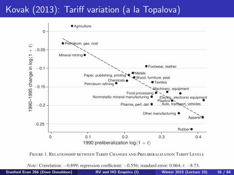
Kovak (2013): Tariff variation (a la Topalova)1968 THE AMERICAN ECONOMIC REVIEW AugusT 2013

and Pavcnik (2005). It was a stated goal of policymakers to reduce tariffs in general, and to reduce the cross-industry variation in tariffs to minimize distortions rela-tive to external incentives (Kume, Piani, and de Souza 2003). This equalizing of tariff levels implies that the tariff changes during liberalization were almost entirely determined by the preliberalization tariff levels. Figure 1 shows that industries with high tariffs before liberalization experienced the greatest cuts, with the correlation between the preliberalization tariff level and change in tariff equaling −0.90. Since the liberalization policy imposed cuts based on a protective structure that was set decades earlier (Kume, Piani, and de Souza 2003), it is unlikely that the tariff cuts were manipulated to induce correlation with counterfactual industry performance or with industrial political influence.20

IV. The Effect of Liberalization on Regional Wages

A. Regional Wage Changes

The model described in Section I considers homogenous labor, in which all work-ers are equally productive and thus receive identical wages in a particular region.

20 It should be noted that the 1990–1995 tariff changes are negatively correlated with the preliberalization 1985–1990 growth in industry employment, indicating that industries that were growing more quickly during 1985–1990 subsequently experienced larger tariff cuts during liberalization in 1990–1995. While this correlation is consistent with strategic behavior in which the “strongest” industries were allowed to face increased international competition, under a counterfactual in which the trends would have continued, such a relationship would impart downward bias to the wage results below, going against finding the positive estimates they exhibit.

Figure 1. Relationship between Tariff Changes and Preliberalization Tariff Levels

Note: Correlation: −0.899; regression coefficient: −0.556; standard error: 0.064; t: −8.73.

Source: Author’s calculations based on data from Kume, Piani, and de Souza (2003).

Petroleum, gas, coal

Agriculture

Mineral mining

Petroleum refiningChemicals

Paper, publishing, printingMetalsWood, furniture, peat

Footwear, leather

Pharma, perf, det

Nonmetallic mineral manufacturing

Textiles

Food processingMachinery, equipment

Plastics

Other manufacturing

Electric, electronic equipment

Rubber

Apparel

Auto, transport, vehicles

–0.25

−0.2

−0.15

−0.1

−0.05

019

90–1

995

chan

ge in

log(1

+ t

)

0 0.1 0.2 0.3 0.4

1990 preliberalization log(1 + t)


Kovak (2013): RTCr changes by region r 1971kovak: measuring regional effects of trade reformvol. 103 no. 5

change. Rio de Janeiro has more weight in the left side of the diagram, particularly in the apparel and food processing industries. Traipu produces agricultural goods almost exclusively, which faced the most positive tariff changes. Thus, although all regions faced the same set of tariff changes across industries, variation in the weight applied to those industries in each region generates the substantial variation seen in Figure 3.

C. Wage-Tariff Relationship

Given empirical estimates of the regional wage changes and region-level tariff changes, it is possible to examine the effect of tariff changes on regional wages predicted by the specific-factors model. I form an estimating equation from (1) as

(7) d ln ( w r ) = ζ 0 + ζ 1 RT C r + ϵ r ,

where d ln( w r ) is the regional wage change described in Section IVA. Since these wage changes are estimates, I weight the regression by the inverse of the standard error of the estimates based on Haisken-DeNew and Schmidt (1997). ζ 1 captures the regional effect of liberalization on real wages between 1991 and 2000. The model predicts

• •

•

•

•

•

•

•

•

•

•

BelémBelém

RecifeRecife

ManausManaus

CuritibaCuritiba

BrasíliaBrasília

SalvadorSalvador

FortalezaFortaleza

São PauloSão Paulo

Porto AlegrePorto Alegre

Belo HorizonteBelo Horizonte

−15% to −8%

−8% to −4%

−4% to −3%

−3% to −1%

−1% to 1.4%

Figure 3. Region-Level Tariff Changes

Notes: Weighted average of tariff changes. See text for details.


Kovak (2013): Main Results1973kovak: measuring regional effects of trade reformvol. 103 no. 5

region-level tariff changes is positive. This implies that microregions facing the larg-est tariff declines experienced slower wage growth than regions facing smaller tariff cuts, as predicted by the model. The estimate in column 1 of 0.404 implies that a region facing a 10 percentage point larger liberalization-induced price decline expe-rienced a 4 percentage point larger wage decline (or smaller wage increase) relative to other regions. The difference between the region-level tariff change in regions at the 5th and 95th percentile was 12.8 percentage points. Evaluated using the col-umn 1 estimate, a region at the 5th percentile experienced a 5.2 percentage point larger wage decline (or smaller wage increase) than a region at the 95th percentile. The addition of state fixed effects in column 2 has almost no effect on the point estimate but absorbs residual variance such that the estimate is now statistically significantly different from zero at the 1 percent level.

The remaining columns of Table 1 examine the effects of deviations from the preferred specification in columns 1 and 2. Columns 3 and 4 omit the labor share adjustment, which in the context of the model is equivalent to assuming that the labor demand elasticities are identical across industries so that the weights in each region are determined only by the industrial distribution of workers. All of the papers in the previous literature follow this approach. In the Brazilian context, the omission of the labor share adjustment has very little effect on the estimates, as they have little effect on the weights across industries. Taking a region × industry pair as an observation, the correlation between the weights with and without labor share adjustment is 0.996.

Columns 5 and 6 include the nontraded sector in the regional tariff change cal-culations, setting the nontraded price change to zero. Footnote 8 lists papers using this approach.26 This change results in a substantial increase in the point estimates,

26 The previous literature does not explicitly make assumptions about the price of nontraded goods but rather includes a zero term for the nontraded sector in the weighted averages used in their empirical analyses. In the con-text of the present model, that is equivalent to assuming zero price change for nontraded goods. However, many

Table 1—The Effect of Liberalization on Local Wages

No labor share Nontraded price Nontraded sectorMain adjustment change set to zero workers’ wages

(1) (2) (3) (4) (5) (6) (7) (8)

Regional tariff change 0.404 0.439 0.409 0.439 2.715 1.965 0.417 0.482Standard error (0.502) (0.146)*** (0.475) (0.136)*** (1.669) (0.777)** (0.497) (0.140)***

State indicators (27) — X — X — X — X

Nontraded sector Omitted X X X X — — X X Zero price change — — — — X X — —

Labor share adjustment X X — — X X X X

R2 0.034 0.707 0.040 0.711 0.112 0.710 0.037 0.763

Notes: 493 microregion observations (Manaus omitted). Standard errors adjusted for 27 state clusters (in parenthe-ses). Weighted by the inverse of the squared standard error of the estimated change in log microregion wage, calcu-lated using the procedure in Haisken-DeNew, and Schmidt (1997).

*** Significant at the 1 percent level. ** Significant at the 5 percent level. * Significant at the 10 percent level.


Dix-Carneiro (Ecta. 2014)

Kovak (2013) assumed that labor was fully and instantaneouslymobile across industries. What about adjustment costs?

Dix-Carneiro (2014) develops and estimates a rich model ofworker-level adjustment costs using remarkable panel data(employee-employer matched data, though the employer dimension isnot featured here, apart from the employer’s industry) from theuniverse of formal sector workers in Brazil from 1986-2005.

Key features:Roy-like model: workers choose which sector to work inBut dynamic: workers have rational expectations over the future pathof wages in each sectorIn addition, wage depends on age and sector-specific experience.Workers are heterogeneous in terms of observables (e.g. gender,education)Cost of switching sectors (different for each pair)

GMM estimation drawing on tools in Lee and Wolpin (Ecta., 2006)


Dix-Carneiro (2014): Counterfactual ResultsTRADE LIBERALIZATION AND LABOR MARKET DYNAMICS 861

FIGURE 4.—Dynamics under Perfect Capital Mobility following the adverse price shock in theHigh-Tech Manufacturing sector illustrated in the left upper panel. The prices of the non-trade-able sectors adjust in equilibrium. The evolution of human capital prices, employment shares,real value added, and aggregate welfare following the shock are subsequently displayed in thatorder.


Dix-Carneiro and Kovak (2014)

Very nice combination of the previous two papers

First, using regional aggregate data (like in Kovak, 2013) estimatedynamic version of Kovak regression:

wrt − wr ,1991 = ρtRTCr + αst + γt(wr ,1990 − wr ,1986) + εrt (11)

Then plot the estimated coefficients ρt over time and compare withend of liberalization period (1995).


Dix-Carneiro and Kovak (2014): Regional Results

Trade Reform and Regional Dynamics Dix-Carneiro and Kovak

Figure 4: Regional log Formal Earnings Premia - 1992-2010

-0.4

-0.1

0.2

0.5

0.8

1.1

1.4

1.7

2

2.3

1992 1993 1994 1995 1996 1997 1998 1999 2000 2001 2002 2003 2004 2005 2006 2007 2008 2009 2010

Each point reflects an individual regression coefficient where the dependent variable is the change in regional log formalearnings premium from 1991 to the year listed on the x-axis, calculated using RAIS. For all years, the independentvariable is the regional tariff change reflecting tariff changes from 1990-1995 (described in the text), with state fixedeffects and pre-trend control. Positive estimates imply larger earnings declines in regions facing larger tariff declines.Vertical bar indicates that liberalization was complete in 1995. Dashed lines show 95 percent confidence intervals.Standard errors adjusted for 112 mesoregion clusters.

43









(2005)



Areas for Future Research

Tracing the short-, medium- and long-run adjustment to tradeliberalizations or other ‘natural experiments’.

Can RV and HO models be unified in the data as the same model withdifferent time horizons?

Ideally one could use firm-level panel data (which we will see lots oflater in the course and in Kalina’s course next quarter).

Trefler (2004 AER) does this well for Canada’s liberalization(CUSFTA), as we will see later in the course. But focus there was onproductivity changes, rather than factor adjustment/mobility.

Try to add capital market adjustment frictions: Caballero-Engel(various), Kline (2008), Bloom (Ecta, 2008)

Further applications of the GL (1989) event-study approach to Tradequestions?









(2005)



Introduction to HO Empirics

The H-O model is probably the most influential model in all of Trade.So how do we assess how useful a description of the real world it is?

One immediate obstacle is that the theory’s predictions aren’t thatprecise.

The 2× 2 model makes precise predictions, but (without putting morestructure on the problem) not much of this generalizes to higherdimensional settings (Ethier (1984, Handbook chapter)).

As we have seen, this is a familiar problem from wider ComparativeAdvantage settings (including the Ricardian model)


What predictions does HO make in general cases?

Recall that assumption on the number of goods (G ) and factors (F )is key:

If G ≤ F , production (and hence trade) is determinate. Hence the‘Goods Content of Trade’ (GCT) (or pattern of trade) is determinate.We will first discuss empirical work that pursues this approach.However, to get empirical traction, this approach usually needs toassume that G = F .

If G > F , production (and hence trade) is indeterminate. But the(Net) Factor Content of Trade (NFCT) is determinate—the HOVprediction. We will (next lecture) discuss empirical work that pursuesthis approach. This has been the more influential of the two directions(but I’m not quite sure why, except for fact that G > F is perhaps howwe’re used to thinking of the world).


Aside: How many goods and factors are there?

Clearly, as we map from this model to the real world, the G ≥≤ Fquestion really hangs on our level of aggregation (every worker isdifferent in some dimension!)

And of course ‘aggregation’ is really just a matter of at what level weassume goods/factors are perfect substitutes so that they can betrivially aggregated.

A different approach is pursued by Bernstein and Weinstein (JIE,2002), who examine whether G ≥ F seems more plausible by testingthe indeterminacy of production (conditional on endowments) in aG > F world.


Introduction to ‘Goods Content’ of Trade Tests

Now we focus on the case of G ≤ F , and ask whether the H-Omodel’s predictions for trade (or output) of goods find support in thedata.

Also called ‘Rybczinski regressions’.

Brief chronology:

Baldwin (1971): not quite the right testLeamer (1984, book): first pure test on trade flowsHarrigan (JIE, 1995): same as Leamer (1984) but on outputHarrigan (AER, 1997): adding technology differencesSchott (AER, 2001): multiple cones of specializationRomalis (AER, 2004) (and Morrow (2009)): actually G > F , butproduction indeterminacy broken by trade costs (and hence lack ofFPE).


H-O Theory with G ≤ F , Part I

Recall the revenue function (for country c):Y c = r c (pc ,V c ) ≡ maxy c{pc .y c : y c ∈ T (V c )}.

Here Y is total GDP, y is the vector of outputs (in each sector), p isthe vector of prices, and T is the technology set.

Then we have (with G ≤ F ): y c = ∇prc (pc ,V c), which is

homogeneous of degree one in V c by CRTS.

Recall that with G > F , this becomes a correspondence (i.e.production is indeterminate), not an equality.

And hence: y c = ∇pV r c (pc ,V c) · V c ≡ Rc (pc ,V c) · V c .

Rc (pc ,V c ) is often called the ‘Rybczinski matrix’.


H-O Theory with G ≤ F , Part II

The prediction y c = Rc (pc ,V c) · V c looks amenable to empiricalwork, at first glance.

Clearly, without any structure on the technology set T , i.e. on R(·),this can’t go anywhere.

Some work (e.g. Kohli (1978, 1990)) has applied structure (e.g. atranslog or generalized Leontief revenue function) and gone from there,using data from one country.

But if you wanted to pool estimates across countries, or don’t observegoods price data in all countries, the equation above offers no guidanceon how to proceed.


H-O Theory with G ≤ F , Part III

A more influential approach has been to further assume that G = F(the so-called ‘even case’). Then:

The factor market clearing conditions imply immediately that(assuming Ac (w c ,V c ) is invertible): y c = [Ac (w c ,V c )]−1V c

So Rc (pc ,V c ) = [Ac (w c ,V c )]−1.

And if we confine attention to an FPE equilibrium (identicaltechnologies (ie Ac (·, ·) = A(·, ·)), no trade costs, no factor intensityreversals, and endowments inside the FPE set) then ‘factor priceinsensitivity’ holds: A(w ,V c ) = A(w). (That is, techniques used arelocally independent of V c .)

Similarly: Rc (pc ,V c ) = R(p) —that is, all countries have the sameRybczinski (or A) matrix.


From Production to Trade

Finally, we can apply the usual trick—of identical and homotheticpreferences—in trade to convert predictions about output intopredictions about trade flows.

Which, when coupled with the assumption of no trade costs, impliesthat:

T c (p,V c ) = R(p) · V c − α(p)Y c

Where α(p) is, as in Lecture 9, the vector of consumption budgetshares at prices p (common to the whole world).


T c (p,V c ) = R(p) · (V c − scV w )

Where sc is country c ’s share of world GDP, and V w is the worldendowment vector.


Baldwin (1971) I

Theory: T c (p,V c ) = R(p) · (V c − scV w )

Baldwin (1971) was the first to explore the implications of thisequation empirically.

He could have either:1 Taken data on T c (p,V c ), R(p) = [A(w)]−1, and (V c − scV w ), to

check this prediction exactly. As we’ll discuss next lecture, one canobtain data on A(w) from input-output accounts.

2 Or, regressed T c (p,V c ) on R(p) = [A(w)]−1 to check whether theestimated coefficients take the same signs/magnitudes as (V c − scV w )

3 Or, regressed T c (p,V c ) on (V c − scV w ) to check whether theestimated coefficients take the same signs/magnitudes asR(p) = [A(w)]−1

Baldwin (1971) did 2. Leamer (1984) did a version of 3.


Baldwin (1971) II

Baldwin (1971) used data:From the US, for 60 industries and 9 factors (K plus 8 types of labor),around 1960.This seems to say that G > F (not G = F ) but since we’re testing thisequation-by-equation, it’s OK if we just happen to be missing the other41 factors (whatever they are!)Data on T c was net exports. (No role for intra-industry trade.)

Results:Unfortunately, Baldwin (1971) actually mistook R(p) = [A(w)] insteadof R(p) = [A(w)]−1, so the results are wrong. But Leamer and Bowen(1981) show that the sign pattern of the estimated coefficients is onlywrong if sign{(AA′)−1} 6= sign{A−1}. And Bowen and Sveikauskas(1992) show that the actual A matrices suggest this isn’t likely to betrue.Results were not really testable (without reliable data on V w ), butseemed reasonable except for one exception: the coefficient on physicalcapital was negative (and everyone thought the US was relativelycapital abundant).


Leamer (1984 book): Set-up

Leamer instead treats (V c − scV w ) as data and regresses T c (p,V c )on (V c − scV w ).

Really, this amounts to estimating the regression equationT c

i =∑F

k=1 βik (V ck − scV w

k ) + εci across countries c , one commodity

i at a time.

The coefficients βik are often called ‘Rybczinski effects’.


Leamer (1984): Data

Leamer (1984) did a huge amount of pioneering work in compilingdata on trade flows and factor endowments.

60 countries, two different years (1958 and 1975)

Goods classifications: Leamer organizes the data into 10 goods,deliberately aggregating over some finer-level data in order to find‘industries’ in which exports appear to flow the same way (withinindustries), and capital-worker and professional worker-all workerratios are similar within industries. (So industries look roughly similaralong taste and technology dimensions.)

Factors: K, 3 types of L, 4 types of land (distinguished by climate),and 3 types of natural resources.

11 Goods (10 plus non-traded goods) and 11 Factors (G = F !)


Leamer (1984): Results and Interpretation I

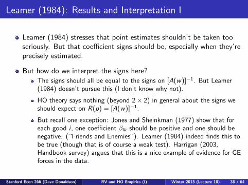
Leamer (1984) stresses that point estimates shouldn’t be taken tooseriously. But that coefficient signs should be, especially when they’reprecisely estimated.

But how do we interpret the signs here?

The signs should all be equal to the signs on [A(w)]−1. But Leamer(1984) doesn’t pursue this (I don’t know why not).

HO theory says nothing (beyond 2× 2) in general about the signs weshould expect on R(p) = [A(w)]−1.

But recall one exception: Jones and Sheinkman (1977) show that foreach good i , one coefficient βik should be positive and one should benegative. (“Friends and Enemies”). Leamer (1984) indeed finds this tobe true (though that is of course a weak test). Harrigan (2003,Handbook survey) argues that this is a nice example of evidence for GEforces in the data.


Leamer (1984): Results and Interpretation II

Leamer (1984) has a great discussion of how we could interpret someof the precisely-estimated coefficients:

For example: in manufacturing, the coefficient on capital is positive(which perhaps seems sensible).

But in manufacturing, the coefficient on land is negative. (Note thatthis is the sort of surprising result—echoing Harrigan’s (2003)comment about evidence for GE forces—you could never find in anindustry-by-industry production function estimation approach.) Why?Perhaps because a country with lots of land specializes in agriculture,and this draws other resources out of manufacturing.

These are plausible interpretations, but there is nothing in general HOtheory that says these need to be true. That is, we don’t know exactlywhere to expect these negative coefficients. The fact that some appearis therefore a fairly weak test.


Harrigan (JIE, 1995) I

Harrigan (1995 and 2003) argues that the real intellectual content ofHO theory concerns production, not consumption, and hence nottrade at all:

The addition of the IHP assumption to convert a prediction aboutproduction into a prediction about trade, he argues, is at best adistraction, and at worse very misleading (since IHP isn’t likely to betrue.)

Of course, that isn’t to imply that enriching the IHP assumption isn’tworth doing if the goal is to explain trade flows.

A key reason for Leamer (1984) to use trade data rather than outputdata was not just his interest in trade—he lacked comparable outputdata across countries. (Trade data has been good and plentiful aroundthe world for centuries longer than any other type of data.) By theearly 1990s, however, the OECD had started to make comparableoutput data available to researchers, so Harrigan uses this.


Harrigan (JIE, 1995) II

So Harrigan (1995) pursues the Leamer (1984) approach using outputdata instead of export data.

The results are similar to Leamer’s.

But he highlights that an overall disappointment is that the R2 isvery low.

In other words, the production-side assumptions made in conventionalHO theory are incapable of capturing much of the variation in outputacross countries and industries (and years).


Harrigan (AER, 1997)

Harrigan (1997) starts from the premise that (what is probably) themost egregious assumption in conventional HO theory is that ofidentical technologies across countries.

But how to build non-identical technologies into the above framework?

That framework rested on the notion that since countries have identicaltechnologies, and face identical goods prices due to free trade, and FPIand FPE hold, R(.) is identical across countries. And we can thereforeestimate R(.) using variation in V c across countries.

Harrigan’s solution was to add more structure to the set-up.

He assumed a particular (but flexible—‘superlative’, in the language ofDiewert (1976)) functional form for the revenue function.


Harrigan (1997): Set-up I

Harrigan assumes a translog revenue function.

To this he adds Hicks-neutral productivity difference in each countryand sector: θc

i .

With the additional restriction that all countries face the same pricesp and that the translog is CRTS (and fixed over time), he derives thefollowing estimation equation:

scit = αit +

F∑k=2

aki ln

(θc

kt

θc1t

)+

G∑j=2

rij ln

(V c

jt

V cjt

)

Here, scit is the share of output of sector i in country c’s GDP in year

t, αit is a sector-year fixed effect, and the parameters aki and rij arethe translog parameters.

It turns out that this revenue function also has implications for factorshares which could be tested in principle.


Harrigan (1997): Set-up II

A complication is the presence of non-traded goods:

That is, there are some elements of the price vector which are notequalized across countries and that will therefore not be absorbed intothe αit fixed effect.

In particular, there will now be terms involving non-traded goods pricesand non-traded sectors’ productivities.

Harrigan (1997) argues that these terms might be soaked up in a fixedeffect at the country-good level, and if not, they might be orthogonalto the terms included above.


Harrigan (1997): Implementation

Harrigan estimates the above equation using a panel of countries andindustries.

He estimates the equation one good at a time (with country and yearfixed effects), but in a SUR sense (since the dependent variable is ashare so all dependent variables sum to one).

Note that the data requirements go beyond Harrigan (1995):Harrigan (1997) requires data on TFP by industry and country.

He also instruments TFP (for fear of classical measurement error),using the average of other countries’ TFPs as the instrument (sectorby sector).


Harrigan (1997): Results488 THE AMERICAN ECONOMIC REVIEW SEPTEMBER 1997

TABLE 5-ESTIMATES OF THE GDP SHARE EQUATIONS, EQUATION (5)

Food Apparel Paper Chemicals Glass Metals Machinery

TFP Food -0.457 0.672 0.144 -0.067 -0.327 0.381 0.005 (-2.01) (4.74) (1.09) (-0.48) (-3.21) (3.55) (0.02)

TFP Apparel 0.672 0.371 0.360 -0.485 -0.057 -0.157 0.597 (4.74) (2.40) (3.14) (-4.25) (-0.65) (-1.92) (3.39)

TFP Paper 0.144 0.360 0.184 -0.104 0.012 -0.003 0.387 (1.09) (3.14) (1.06) (-0.93) (0.13) (-0.04) (2.34)

TFP Chemicals -0.067 -0.485 -0.104 2.025 -0.060 -0.029 -1.198 (-0.48) (-4.25) (-0.93) (11.9) (-0.72) (-0.29) (-5.32)

TFP Glass -0.327 -0.057 0.012 -0.060 0.369 -0.107 -0.174 (-3.21) (-0.65) (0.13) (-0.72) (3.96) (-1.82) (-1.26)

TFP Metals 0.381 -0.157 -0.003 -0.029 -0.107 0.618 -0.583 (3.55) (-1.92) (-0.04) (-0.29) (-1.82), (4.88) (-3.00)

TFP Machinery 0.005 0.597 0.387 -1.198 -0.174 -0.583 3.583 (0.02) (3.39) (2.34) (-5.32) (-1.26) (-3.00) (6.06)

Prod. durables 1.305 0.940 -0.016 1.186 0.358 0.193 0.913 (6.90) (6.57) (-0.14) (5.78) (3.89) (0.96) (1.91)

Nonres. const. -0.195 -0.353 0.157 -1.530 -0.244 -0.066 -1.754 (-0.68) (-1.68) (0.90) (-5.26) (-1.70) (-0.24) (-2.44)

High-ed. workers -0.170 -0.663 -0.219 -0.002 -0.190 -0.503 -2.114 (-1.34) (-7.16) (-2.98) (-0.02) (-3.18) (-3.93) (-6.60)

Medium-ed. workers 0.682 0.688 -0.035 -0.889 0.378 -0.210 1.013 (3.47) (4.88) (-0.31) (-4.44) (4.20) (-1.10) (2.11)

Low-ed. workers -0.020 0.102 -0.148 -0.397 -0.103 -0.224 1.820 (-0.14) (0.99) (-1.78) (-2.68) (-1.53) (-1.55) (5.22)

Arable land -1.602 -0.714 -0.261 1.631 -0.200 0.809 0.123 (-5.27) (-3.09) (1.43) (5.10) (-1.32) (2.64) (0.14)

Notes: Estimation results are listed columns, with t-statistics in parentheses. The dependent variable is the percentage share of the industry in GDP. All explanatory variables are in logarithms, and are listed as rows. Country and year fixed effects are not shown. There are 203 observations in regression. For further details on this table, see the text.

of relative factor supplies obscures the equilibrium relationship that was apparent when adjustment was assumed to be immediate, as it is in Table 5.

To help understand the size of the effects reported in Tables 5 and 6, Table 7 reports standardized coefficients, which are transfor- mations of the regression coefficients into units of sample standard deviations.'2 For ex-

ample, a standardized coefficient of 1.3 means that a one-standard-deviation increase in the explanatory variable will increase the dependent variable by 1.3 standard deviations. The standardized coefficients corresponding to Ta- ble 5 are reported in columns A of Table 7. Columns B of Table 7 report long-run standardized coefficients, where each slope is first divided by 1 - X to convert it into a long-run effect. Numbers are in boldface if the corresponding slope in Table 5 or 6 is significantly different from zero at the 10-percent level. The estimated long-run, own-TFP effects in columns B are invariably larger than the effects in columns A; generally, a one-standard-

2 Standardized coefficients are often known as "beta" coefficients. Standardized coefficients are formed by mul- tiplying the regression slope by the standard deviation of the explanatory variable and dividing by the standard deviation of the dependent variable.


Harrigan (1997): Interpretation

The overall fit (R2), including fixed effects, is now (relative toHarrigan, 1995) quite high: 0.95ish.

Leaves overall message that in fitting a world-wide revenue function,technology differences are important. As we will see next lecture, thisechoes a persistent theme in the HOV literature, post-Trefler (1993).

As theory would predict, the own-TFP effects (the bold diagonals) arealmost always positive and statistically significant.

As theory would predict, some cross-TFP, and cross-endowmentcoefficients are negative, but the location of these negativecoefficients isn’t very stable across specifications (see other tables).


Post-Harrigan (1997) I

Harrigan has room for non-FPE, but not for non-‘conditional FPE’ (inthe language of Trefler (1993, JPE) that we will see in next lecture).

Put another way,ac

Ki

acLi

should be a constant for any two factors (eg K

and L), within any good i and country c .

However, as will see next lecture, Davis and Weinstein (2001, AER)

find that in a regression likeac

Ki

acLi

= βi + β K c

Lc , the coefficient β is usually

large and statistically significant. (See also Dollar, Wolff and Baumol(1988, AER).)

That is, for some reason, even the relative techniques that countriesuse are affected by local relative endowments.

This stands in contrast to a HO model with Hicks-neutral TFPdifferences across countries and sectors.


Post-Harrigan (1997) II

Ways to rationalize this:1 Country-industry technology differences are not Hicks-neutral. This is

probably true, but hasn’t generated much work (in ‘goods content’ oftrade tests).

2 Trade costs prevent any sort of FPE (i.e. different countries facedifferent pc ’s). This is also surely true (as we’ll see in a later lecture,trade costs appear to be very high). Romalis (2004) introduces tradecosts into a special sort of (essentially 2-country) HO model to makeprogress here. Morrow (2009) extends this to include technologydifferences.

3 Countries are not all in the same cone of diversification (i.e. inside the‘conditional FPE set’). Note that same cone of diversification meansthat all countries are incompletely specialized (i.e. all produce some ofall goods), which sounds counterfactual. Schott (AER, 2003) builds onLeamer (JPE, 1987) and looks at whether Rybczinski regressions fitbetter if we allow countries to be in different cones.







3 Appendix: More on the Ricardo-Viner model (for reading athome)

1 Factor price responses to goods price changes:1 Stock market event study approach: Grossman and Levinsohn

(1987)2 Political economy approaches: Magee (1980), Mayda and Rodrik

(2005)2 GNP function approach:

1 Kohli (1993)Stanford Econ 266 (Dave Donaldson) RV and HO Empirics (I) Winter 2015 (Lecture 10) 50 / 64

Factor Price Responses to Goods Price Changes

The classic distinction between the RV and HO models concerns theirimplications for how factor incomes respond to trade liberalization.

That is, how do factor prices respond to changes in goods prices (the‘Stolper-Samuelson derivative’: dw

dp )?In RV model, as p falls in a sector, prices of factors specific to thatsector fall too. Factor incomes are tied to the fate of the sector inwhich they work.In HO model, as p falls, factor incomes are governed by full GEconditions. Factor prices may fall or rise (or with many sectors wemight expect them not to move much).

This distinction drives the empirical approach of a number of papersconcerned with testing the RV vs the HO model:

Wages: Grossman (1987), Abowd (1987)Capital returns: Grossman and Levinsohn (AER, 1989)Lobbying behavior: Magee (1980)Opinions about free trade: Mayda and Rodrik (EER, 2005)


Grossman and Levinsohn (1989)

Testing the effect of goods price changes on factor returns:

Using wages is attractive: there is (probably) something closer to a‘spot market’ (at which we observe the going price) for labor thanthere is for machines.

Using capital returns is also attractive: Can (with some assumptions)use data from stock markets, which provides high quality andhigh-frequency data, as well as the usual opportunities for an ‘eventstudy’ approach. (We are perhaps more likely to believe this is asetting where prices are set by forward-looking, rational agents facingsevere arbitrage pressures.)

In an innovative paper, GL (1989) follow the latter approach.


GL (1989): Setup

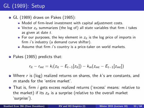
GL (1989) draws on Pakes (1985):Model of firm-level investment with capital adjustment costs.Vector zit summarizes (the log of) all state variables that firm i takesas given at date t.For our purposes, the key element in zit is the log price of imports infirm i ’s industry (a demand curve shifter).Assume that firm i ’s country is a price-taker on world markets.

Pakes (1985) predicts that:

rit − rmt = ki (zit − Et−1[zit ])− km(zmt − Et−1[zmt ])

Where r is (log) realized returns on shares, the k ’s are constants, andm stands for the ‘entire market’.

That is, firm i gets excess realized returns (‘excess’ means: relative tothe market) if its zit is a surprise (relative to the overall market‘surprise’).


GL (1989): Implementation I

The key challenge is to construct measures of ‘surprises’:zit − Et−1[zit ].

Import prices: GL model these as a multivariate autoregressive processin (lagged) import prices, foreign wages, and exchange rates. Once thisis estimated, the residuals of the process can be interpreted as‘surprises’.

Other elements of z : domestic input prices (domestic energy prices anddomestic wages), domestic macro variables (GNP, PPI, M1 Supply).All are converted into ‘surprises’ through a VAR.

Surprises to ‘market’ (m): use same variables as above, but use averagemarket import price rather than firm i ’s own industry’s import price.


GL (1989): Implementation II

The result is a regression of excess returns (rit − rmt) on ‘surprises’(‘NEWS’ in GL(1989) notation) to:

Import prices in firm i ’s industry (‘PSNEWS).Import prices in market, on average.Domestic input prices.Domestic macro variables.

RV model predicts that coefficient on PSNEWS is positive. Simplecalibration suggests coefficient in this model should be just aboveone.

If capital could instantaneously reallocate across industries inresponse to surprises (as in H-O model) then the coefficient onPSNEWS would be zero.


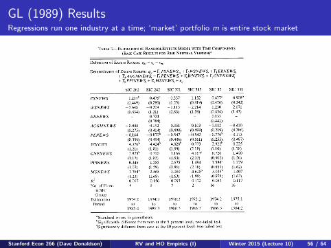
GL (1989) ResultsRegressions run one industry at a time; ‘market’ portfolio m is entire stock market

VOL. 79 NO. 5 GROSSMAN AND LEVINSOHN: STOCK MARKET RETURN TO CAPITAL 1077

TABLE 3 -ESTIMATION OF RANDOM-EFFECTS MODEL WITH TiME COMPONENTS

(BASE CASE RESULTS FOR RISK NEUTRAL VERSION)a

Definition of Excess Return: qit = rit - rm,

Determinants of Excess Return: qit = F, PSNEWS,1, + F2WSNEWS, + F3ERNEWS, + h4A GGMNE WS, + F5PENE WS, + F6 WNE WS, + F7GNPNEWS, + F8PPINE WS, + F9MSNE WS, + vP,

SIC 262 SIC 242 SIC 301 SIC 345 SIC 32 SIC 331

PSNEWS 1.217b 0.476c - 0.357 1.152 0.827c 0.908b

(0.449) (0.280) (1.25) (0.819) (0.476) (0.343)

WSNEWS - 0.648 - 0.209 -1.115 - 2.214 1.230 2.071

(0.834) (1.21) (2.83) (1.59) (0.854) (1.43)

ERNEWS - 0.724 - - 0.133 -

(0.784) (0.442)

AGGMNEWS - 0.044 0.192 0.351 0.103 - 0.112 -0.410

(0.275) (0.414) (0.498) (0.499) (0.219) (0.386)

PENEWS - 0.164 - 0.870b - 0.547 - 0.542 - 0.776b - 0.173

(0.356) (0.454) (0.486) (0.561) (0.255b (0.487)

WNEWS 4.376b 4.424b 4.828 0.773 2.922 0.225

(1.21) (1.81) (1.89) (2.18) (1.10) (1.78)

GNPNEWS 2.825b 0.310 1.166 4.167c 0.726 1.470

(1.17) (1.83) (1.83) (2.03) (0.902) (1.56)

PPINEWS 0.345 1.585 2.675 1.494 1.584c 1.279

(1.07) (1.59) (1.86) (2.18) (0.853) (1.62)

MSNEWS 2.784b 2.565 3.080c 4.628b 3.029 1.407

(1.23) (1.68) (1.63) (1.99) (0.978) (1.62)

R 2 0.097 0.156 0.093 0.172 0.083 0.117

No. of Firms 9 5 7 2 16 16 in SIC Group

Estimation 1974:2 1974:3 1976:3 1975:2 1974:2 1975:1

Period to to to to to to

1985:4 1986:3 1986:3 1986:3 1986:3 1984:2

a Standard errors in parentheses.

bSignificantly diferent from zero at the 5 percent level, two-tailed test.

'Significantly different from zero at the 10 percent level, two-tailed test.

from a CAPM equation.'7 In creating these tables, we have excluded ERNEWS from the regressions for SIC 262, SIC 301, SIC 345, and SIC 331. The inclusion of this variable in the model follows from the hypothesis that the exchange rate serves as a predictor of future import prices. Conversely, the model implies that if exchange rates do not help to predict domestic-currency import prices, F3 and Q3 should be zero. The results in Table

2 show that no lags of the exchange rate were significant in the autoregressions for p,* in four of the industries. Consequently, we dropped ERNEWS from these regressions.

The model performs admirably, explain- ing in each case between 8 and 18 percent of the variance of excess returns. In each industry, several of the news variables are found to have significant impacts on (either measure of) excess returns. The coefficient on PSNEWS, which theory predicts should be positive, is found indeed to be positive in five of the six industries when the assumption of risk-neutrality is imposed, and in all six cases when it is not. The effects of shocks to aggregate import competition on the market rate of return are less pronounced; we

17The estimated values of /, used in the construction of ,, (with their respective standard errors) were as follows: SIC 262, 1.116 (0.108); SIC 242, 1.502 (0.135); SIC 301, 1.439 (0.193); SIC 345, 1.358 (0.210); SIC 32, 1.080 (0.099): SIC 331. 1.081 (0.169).


Magee (1980): “Simple Tests of the S-S Theorem”

Magee (1980) collects data from testimony given in a Congressionalcommittee on the Trade Reform Act of 1973.

29 Trade associations (“representing management”) and 23 laborunions expressed whether they were for either freer trade or greaterprotection. These groups belong to industries.

Striking findings, in favor of RV model (and against simple version ofthe S-S Theorem/HO model):

1 K and L tend to agree on trade policy within an industry (in 19 out of21 industries).

2 Each factor is not consistent across industries. (Consistency is rejectedfor K, but not for L).

3 The position taken by a factor (in an industry) is correlated with theindustry’s trade balance.

Relatedly: As we shall see later in the course, lobbying models (mostprominently: Grossman and Helpman (AER, 1994)) typically makethe RV assumption for tractability.

Goldberg and Maggi (AER, 1999) find empirical support for this in theUS tariff structure.


Mayda and Rodrik (EER, 2005)

Mayda and Rodrik (2005) exploit internationally-comparable surveys(such as the World Values Survey) to look at how national attitudesto free trade differ across, and within, countries.

Findings support both HO and RV models:

HO: People in a country are more likely to oppose trade reform if theyare relatively skilled and their country is relatively skill-endowed.(Recall S-S: trade reform favors scarce factors.)

RV: People in import-competing industries are more likely to opposetrade reform (than those in non-traded industries).


Kohli (JIE, 1993): Introduction

Kohli (1993) pursues a different distinction between RV and HO.

Basic idea:

In a standard neoclassical economy, profit maximization leads tomaximization of the total value of ouptut (or ‘GNP’).

Further, the revenue (or ‘GNP’) function summarizes all informationabout the supply-side of the economy.

The solution to revenue maximization problem should depend, in someway, on whether the maximization is ‘constrained’ (some factor cannotmove across sectors, ie the RV model) or ‘unconstrained’ (all factorscan move, ie the HO model).

Kohli (1993) searches for a way to isolate how constrained andunconstrained GNP functions look in general, and then tests for this.


Kohli (1993): Details I

Kohli (1993) works with the (net) restricted GNP/revenue function(Diewert, 1974):

R(p1, p2,w ,K ) ≡ maxy1,y2,L

{p1y1 + p2y2 − wL : (y1, y2, L,K ) ∈ T}

Where p is the goods price (in sector 1 or 2), y is output, L and K arelabor and capital endowments, w is the wage, and T is the feasibletechnology set.Here ‘restricted’ means that the allocation of K is fixed across sectors.Only L can be allocated to maximize (net) revenue/GNP.

This is homogeneous (of degree 1) in K :R(p1, p2,w ,K ) = r(p1, p2,w)K .


Kohli (1993): Details II

Kohli makes one assumption that is not in the usual RV model:relative stocks of industry-specific capital are constant over time.

If this is true, then it is as if each industry was using a (different)amount of some public input.

Kohli (1985) shows that if there is such a public input, and it is K ,then the aggregate restricted revenue function is additively separableacross industries:

R(p1, p2,w ,K ) = R1(p1,w ,K ) + R2(p2,w ,K )

Note that, unlike in the general case, ∂2R∂p1∂p2

= 0. This is what Kohli(1993) tries to test.


Kohli (1993): Details III

To make progress, Kohli (1993) needs to assume a functional form forR(.).

In particular, he works with the ‘Generalized Leontief’ productionfunction (Diewert, 1971) with disembodied technological change:

R(p1, p2,w ,K ) = [b11p1 + b22p2 + bLLweµLt + 2b12

√p1√p2

+ 2b1L√p1√we−1/2µLt

+ 2b2L√p2√we−1/2µLt ]KeµK t

Note that the key testable restriction of the SF model is now∂2R

∂p1∂p2= b12 = 0.

Kohli tests this using aggregate US data from 1948-1987.


Kohli (1993) Results ITwo ‘goods’ (1 and 2) are Consumption and Investment. Also presented are joint costfunction estimates (dual to the revenue function).

U. Kohli, The specijk-[actors model 129

Table 2

Parameter estimates (t-values in parentheses).

Restricted joint cost function

JP ANJIPO

alI 932.15 (16.30)

act 8,541.U (20.09)

aKX 6,774.0 (15.29)

arc 311.31 (2.86)

alK -766.12 (-7.18)

acK - 6.949.5 (- 16.67)

VL 0.01052 (12.01)

l.0Q2.8 (18.71)

X,919.6 (21.76)

6,557.4 (15.31)

- 527.22 (-8.83)

- 6,994.4 (~ 16.66)

0.00967 (10.06)

PK 0.00203 0.00335 (3.25) (6.77)

LL - 494.59 -498.19

R: 0.94849 0.9453 1

Revenue function

JP ANJIPQ

h l, 2,000.4 1,964.5 (6.59) (6.54)

kc 4,734.8 4,730.6 (24.37) (24.56)

h LL 1,982.9 2,144.7 (4.71) (6.25)

b,c - 103.59 ( ~ 0.66)

h l,, - 1,170.2 - L238.4 ( - 3.85) ( - 4.25)

h CL - 2.485.2 - 2,58 1 .O (~ 10.12) (-13.31)

PI. 0.01504 0.01500 ( 18.90) (18.19)

PK 0.00196 0.00216

(4.04) (5.42)

LL - 505.20 - 505.42

R: 0.93852 0.93831

Notes: JP: joint production ANJIPQ: almost non-jointness in input prices and quantities.

Table 3

Specific-factors model: tests statistics.

HI Ho Restriction Test statistic df x20.95 x20.99

(i) CL restricted joint cost function JP ANJIQP a,,=0 7.20 1 3.84 6.63

(ii) GL revenue function JP ANJIQP h,,=O 0.44 1 3.84 6.63

Notes: JP: joint production. ANJIPQ: almost non-jointness in input prices and quantities.

elasticity estimates are reported for selected years in table 4. As expected, an increase in an output price increases the supply of that good and reduces the production of the other one, and it increases the rental price of labor (the mobile factor), but less than proportionately; an increase in the endowment of labor increases the supply of both outputs, reduces its rental price, and raises the price of capital services; an increase in the endowment of capital (the immobile or ‘public’ input) increases the supply of at least one output (it


Kohli (1993) Results IISo the RV model’s restriction is not rejected when using the revenue approach. (It is whenusing the joint cost approach, but in an open economy it is perhaps more sensible to takeprices as exogenous (revenue approach) than quantities as exogenous (cost approach).)

U. Kohli, The specijk-[actors model 129

Table 2

Parameter estimates (t-values in parentheses).

Restricted joint cost function

JP ANJIPO

alI 932.15 (16.30)

act 8,541.U (20.09)

aKX 6,774.0 (15.29)

arc 311.31 (2.86)

alK -766.12 (-7.18)

acK - 6.949.5 (- 16.67)

VL 0.01052 (12.01)

l.0Q2.8 (18.71)

X,919.6 (21.76)

6,557.4 (15.31)

- 527.22 (-8.83)

- 6,994.4 (~ 16.66)

0.00967 (10.06)

PK 0.00203 0.00335 (3.25) (6.77)

LL - 494.59 -498.19

R: 0.94849 0.9453 1

Revenue function

JP ANJIPQ

h l, 2,000.4 1,964.5 (6.59) (6.54)

kc 4,734.8 4,730.6 (24.37) (24.56)

h LL 1,982.9 2,144.7 (4.71) (6.25)

b,c - 103.59 ( ~ 0.66)

h l,, - 1,170.2 - L238.4 ( - 3.85) ( - 4.25)

h CL - 2.485.2 - 2,58 1 .O (~ 10.12) (-13.31)

PI. 0.01504 0.01500 ( 18.90) (18.19)

PK 0.00196 0.00216

(4.04) (5.42)

LL - 505.20 - 505.42

R: 0.93852 0.93831

Notes: JP: joint production ANJIPQ: almost non-jointness in input prices and quantities.

Table 3

Specific-factors model: tests statistics.

HI Ho Restriction Test statistic df x20.95 x20.99

(i) CL restricted joint cost function JP ANJIQP a,,=0 7.20 1 3.84 6.63

(ii) GL revenue function JP ANJIQP h,,=O 0.44 1 3.84 6.63

Notes: JP: joint production. ANJIPQ: almost non-jointness in input prices and quantities.

elasticity estimates are reported for selected years in table 4. As expected, an increase in an output price increases the supply of that good and reduces the production of the other one, and it increases the rental price of labor (the mobile factor), but less than proportionately; an increase in the endowment of labor increases the supply of both outputs, reduces its rental price, and raises the price of capital services; an increase in the endowment of capital (the immobile or ‘public’ input) increases the supply of at least one output (it


stanford econ 266: international trade lecture 10...

Documents