econ 266 international trade | lecture 1 | comparative...
TRANSCRIPT
Econ 266 International Trade— Lecture 1 —
Comparative Advantage and Gains from Trade
Stanford Econ 266 (Donaldson)
Winter 2015 (Lecture 1)
Stanford Econ 266 (Donaldson) CA and GT Winter 2015 (Lecture 1) 1 / 39
Today’s Plan
1 Course logistics
2 A Brief History of the Field
3 Neoclassical Trade: Standard Assumptions
4 Neoclassical Trade: General Results
1 Gains from Trade2 Law of Comparative Advantage
Stanford Econ 266 (Donaldson) CA and GT Winter 2015 (Lecture 1) 2 / 39

Course Logistics
Lecture: Monday and Wednesday 11:30AM-1:20PM
Instructor: Dave Donaldson
Office: Landau 327Email: [email protected] hours: just email me
Stanford Econ 266 (Donaldson) CA and GT Winter 2015 (Lecture 1) 3 / 39

Course Logistics
No required textbooks, but you will frequently find it helpful to referto:
Dixit and Norman, Theory of International TradeFeenstra, Advanced International Trade: Theory and Evidence
Stanford Econ 266 (Donaldson) CA and GT Winter 2015 (Lecture 1) 4 / 39

Course Logistics
Course requirements:
15 short ‘paper responses’ (roughly one per week): 50% of the coursegradeOne mock referee report: 20% of the course gradeOne research proposal: 30% of the course grade
Stanford Econ 266 (Donaldson) CA and GT Winter 2015 (Lecture 1) 5 / 39
Course Logistics
Course outline:
1 General setup (gains from trade, comparative advantage) [2 lectures]
2 Ricardian and Assignment Models [5 lectures]
3 “New” trade theory (trade with increasing returns to scale) [2 lectures]
4 Firm-level Trade [4 lectures]
5 Gravity Models [3 lectures]
6 Economic Geography [3 lectures]
Stanford Econ 266 (Donaldson) CA and GT Winter 2015 (Lecture 1) 6 / 39
Today’s Plan
1 Course logistics
2 A Brief History of the Field
3 Neoclassical Trade: Standard Assumptions
4 Neoclassical Trade: General Results
1 Gains from Trade2 Law of Comparative Advantage
Stanford Econ 266 (Donaldson) CA and GT Winter 2015 (Lecture 1) 7 / 39
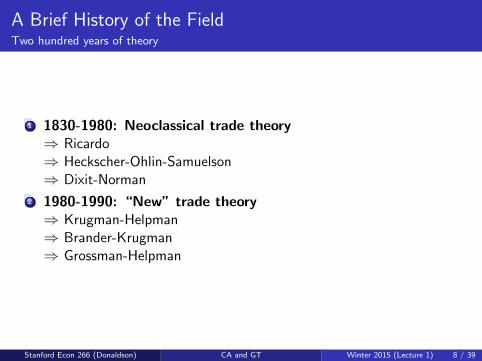
A Brief History of the FieldTwo hundred years of theory
1 1830-1980: Neoclassical trade theory⇒ Ricardo⇒ Heckscher-Ohlin-Samuelson⇒ Dixit-Norman
2 1980-1990: “New” trade theory⇒ Krugman-Helpman⇒ Brander-Krugman⇒ Grossman-Helpman
Stanford Econ 266 (Donaldson) CA and GT Winter 2015 (Lecture 1) 8 / 39
A Brief History of the FieldThe discovery of trade data
1 1990-2000: Empirical trade
2 2000-2010: Firm-level heterogeneity
Stanford Econ 266 (Donaldson) CA and GT Winter 2015 (Lecture 1) 9 / 39

A Brief History of the FieldWhere are we now?
Strong convergence of theory and empirics
Wide range of topics under study from both theoretical and empiricalperspectives (offshoring, multinationals, growth, innovation, tradepolicy, international institutions (GATT/WTO), political economy)
Remarkable growth of new data sources (multi-origin sourcing offirms, multi-destination sales of firms, multi-product sourcing/sales offirms, household scanner data, better price data, firms, firms matchedto matched firms, workers matched to firms, remote sensing,multinationals) often particularly rich in developing countries
Heightened integration of intra-national and inter-nationaltrade/spatial issues (e.g. richer notion of space; allowing for factormobility)
Stanford Econ 266 (Donaldson) CA and GT Winter 2015 (Lecture 1) 10 / 39
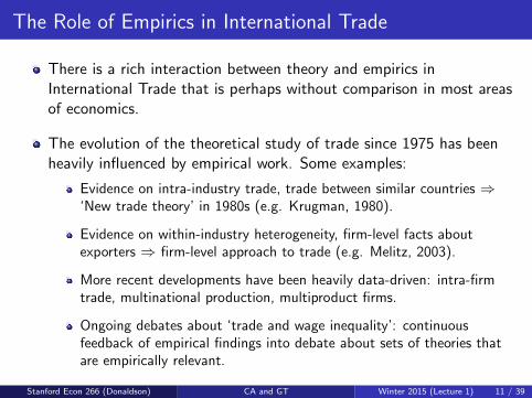
The Role of Empirics in International Trade
There is a rich interaction between theory and empirics inInternational Trade that is perhaps without comparison in most areasof economics.
The evolution of the theoretical study of trade since 1975 has beenheavily influenced by empirical work. Some examples:
Evidence on intra-industry trade, trade between similar countries ⇒‘New trade theory’ in 1980s (e.g. Krugman, 1980).
Evidence on within-industry heterogeneity, firm-level facts aboutexporters ⇒ firm-level approach to trade (e.g. Melitz, 2003).
More recent developments have been heavily data-driven: intra-firmtrade, multinational production, multiproduct firms.
Ongoing debates about ‘trade and wage inequality’: continuousfeedback of empirical findings into debate about sets of theories thatare empirically relevant.
Stanford Econ 266 (Donaldson) CA and GT Winter 2015 (Lecture 1) 11 / 39
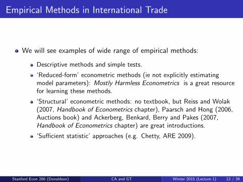
Empirical Methods in International Trade
We will see examples of wide range of empirical methods:
Descriptive methods and simple tests.
‘Reduced-form’ econometric methods (ie not explicitly estimatingmodel parameters): Mostly Harmless Econometrics is a great resourcefor learning these methods.
‘Structural’ econometric methods: no textbook, but Reiss and Wolak(2007, Handbook of Econometrics chapter), Paarsch and Hong (2006,Auctions book) and Ackerberg, Benkard, Berry and Pakes (2007,Handbook of Econometrics chapter) are great introductions.
‘Sufficient statistic’ approaches (e.g. Chetty, ARE 2009).
Stanford Econ 266 (Donaldson) CA and GT Winter 2015 (Lecture 1) 12 / 39
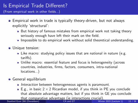
Is Empirical Trade Different?(From empirical work in other fields...)
Empirical work in trade is typically theory-driven, but not alwaysexplicitly ‘structural’:
But history of famous mistakes from empirical work not taking theoryseriously enough have left their mark on the field.Impossible to do empirical work without solid theoretical understanding.
Unique tension:
Like macro: studying policy issues that are national in nature (e.g.tariffs).Unlike macro: essential feature and focus is heterogeneity (acrosscountries, industries, firms, factors, consumers, intra-nationallocations...)
General equilibrium
Interaction between heterogeneous agents is paramount.E.g., in basic 2× 2 Ricardian model, if you think in PE you concludethat absolute advantage matters, but if you think in GE you concludethat comparative advantage (ie interactions crucial).
Stanford Econ 266 (Donaldson) CA and GT Winter 2015 (Lecture 1) 13 / 39

How Do You Do GE Empirics?A common theme in this course
Other heavily empirical fields are rarely forced to (or choose to)grapple with GE.
But there are some great exceptions that include:
Labor: Heckman, Lochner and Taber (AERPP, 1998). Peer effectsliterature (e.g. Manski, Restud 1993). Acemoglu, Autor and Lyle (JPE2004) on large labor supply shock. National-level (e.g. Borjas) vscity-level (e.g. Card) approach to immigration. Crepon et al (2012QJE) on labor market policies.Macro: Caballero-Engel (various), Bloom (Ecta 2007).PF/Health: Finkelstein (QJE 2007) on individual-level vs aggregate(state)-level estimated effects of medicare.Development: Miguel and Kremer (Ecta 2004) on de-wormingspillovers across children within villages.IO: Strategic interactions between firms within industries (Ericsson andPakes (Restud, 1995); Bajari, Benkard and Levin (Ecta, 2007); Bajari,Hong and Nekipelov (2010) survey of game estimation literature; andmany more).
Stanford Econ 266 (Donaldson) CA and GT Winter 2015 (Lecture 1) 14 / 39
Today’s Plan
1 Course logistics
2 A Brief History of the Field
3 Neoclassical Trade: Standard Assumptions
4 Neoclassical Trade: General Results
1 Gains from Trade2 Law of Comparative Advantage
Stanford Econ 266 (Donaldson) CA and GT Winter 2015 (Lecture 1) 15 / 39
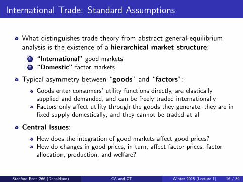
International Trade: Standard Assumptions
What distinguishes trade theory from abstract general-equilibriumanalysis is the existence of a hierarchical market structure:
1 “International” good markets2 “Domestic” factor markets
Typical asymmetry between “goods” and “factors”:
Goods enter consumers’ utility functions directly, are elasticallysupplied and demanded, and can be freely traded internationallyFactors only affect utility through the goods they generate, they are infixed supply domestically, and they cannot be traded at all
Central Issues:
How does the integration of good markets affect good prices?How do changes in good prices, in turn, affect factor prices, factorallocation, production, and welfare?
Stanford Econ 266 (Donaldson) CA and GT Winter 2015 (Lecture 1) 16 / 39
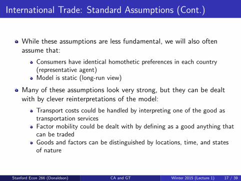
International Trade: Standard Assumptions (Cont.)
While these assumptions are less fundamental, we will also oftenassume that:
Consumers have identical homothetic preferences in each country(representative agent)Model is static (long-run view)
Many of these assumptions look very strong, but they can be dealtwith by clever reinterpretations of the model:
Transport costs could be handled by interpreting one of the good astransportation servicesFactor mobility could be dealt with by defining as a good anything thatcan be tradedGoods and factors can be distinguished by locations, time, and statesof nature
Stanford Econ 266 (Donaldson) CA and GT Winter 2015 (Lecture 1) 17 / 39
Neoclassical Trade: Standard Assumptions
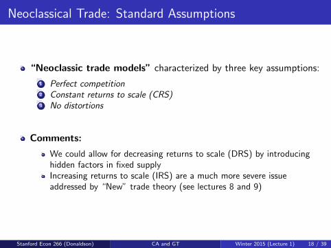
“Neoclassic trade models” characterized by three key assumptions:
1 Perfect competition2 Constant returns to scale (CRS)3 No distortions
Comments:
We could allow for decreasing returns to scale (DRS) by introducinghidden factors in fixed supplyIncreasing returns to scale (IRS) are a much more severe issueaddressed by “New” trade theory (see lectures 8 and 9)
Stanford Econ 266 (Donaldson) CA and GT Winter 2015 (Lecture 1) 18 / 39
Today’s Plan
1 Course logistics
2 A Brief History of the Field
3 Neoclassical Trade: Standard Assumptions
4 Neoclassical Trade: General Results
1 Gains from Trade2 Law of Comparative Advantage
Stanford Econ 266 (Donaldson) CA and GT Winter 2015 (Lecture 1) 19 / 39
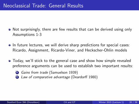
Neoclassical Trade: General Results
Not surprisingly, there are few results that can be derived using onlyAssumptions 1-3
In future lectures, we will derive sharp predictions for special cases:Ricardo, Assignment, Ricardo-Viner, and Heckscher-Ohlin models
Today, we’ll stick to the general case and show how simple revealedpreference arguments can be used to establish two important results:
1 Gains from trade (Samuelson 1939)2 Law of comparative advantage (Deardorff 1980)
Stanford Econ 266 (Donaldson) CA and GT Winter 2015 (Lecture 1) 20 / 39
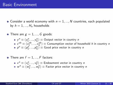
Basic Environment
Consider a world economy with n = 1, ...,N countries, each populatedby h = 1, ...,Hn households
There are g = 1, ...,G goods:
yn ≡ (yn1 , ..., ynG ) ≡ Output vector in country n
cnh ≡ (cnh1 , ..., cnhG ) ≡ Consumption vector of household h in country npn ≡ (pn1 , ..., pnG ) ≡ Good price vector in country n
There are f = 1, ...,F factors:
vn ≡ (vn1 , ..., vnF ) ≡ Endowment vector in country nwn ≡ (wn
1 , ...,wnF ) ≡ Factor price vector in country n
Stanford Econ 266 (Donaldson) CA and GT Winter 2015 (Lecture 1) 21 / 39
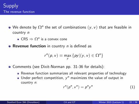
SupplyThe revenue function
We denote by Ωn the set of combinations (y , v) that are feasible incountry n
CRS ⇒ Ωn is a convex cone
Revenue function in country n is defined as
rn(p, v) ≡ maxypy |(y , v) ∈ Ωn
Comments (see Dixit-Norman pp. 31-36 for details):
Revenue function summarizes all relevant properties of technologyUnder perfect competition, yn maximizes the value of output incountry n:
rn(pn, vn) = pnyn (1)
Stanford Econ 266 (Donaldson) CA and GT Winter 2015 (Lecture 1) 22 / 39
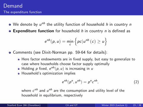
DemandThe expenditure function
We denote by unh the utility function of household h in country n
Expenditure function for household h in country n is defined as
enh(p, u) = minc
pc |unh (c) ≥ u
Comments (see Dixit-Norman pp. 59-64 for details):
Here factor endowments are in fixed supply, but easy to generalize tocase where households choose factor supply optimallyHolding p fixed, enh(p, u) is increasing in uHousehold’s optimization implies
enh(pn, unh) = pncnh, (2)
where cnh and unh are the consumption and utility level of thehousehold in equilibrium, respectively
Stanford Econ 266 (Donaldson) CA and GT Winter 2015 (Lecture 1) 23 / 39
Today’s Plan
1 Course logistics
2 A Brief History of the Field
3 Neoclassical Trade: Standard Assumptions
4 Neoclassical Trade: General Results
1 Gains from Trade2 Law of Comparative Advantage
Stanford Econ 266 (Donaldson) CA and GT Winter 2015 (Lecture 1) 24 / 39
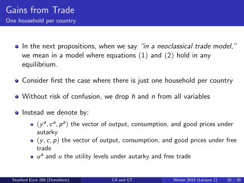
Gains from TradeOne household per country
In the next propositions, when we say “in a neoclassical trade model,”we mean in a model where equations (1) and (2) hold in anyequilibrium.
Consider first the case where there is just one household per country
Without risk of confusion, we drop h and n from all variables
Instead we denote by:
(ya, ca, pa) the vector of output, consumption, and good prices underautarky(y , c , p) the vector of output, consumption, and good prices under freetradeua and u the utility levels under autarky and free trade
Stanford Econ 266 (Donaldson) CA and GT Winter 2015 (Lecture 1) 25 / 39
Gains from TradeOne household per country
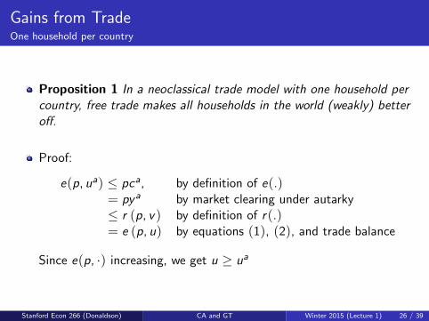
Proposition 1 In a neoclassical trade model with one household percountry, free trade makes all households in the world (weakly) betteroff.
Proof:
e(p, ua) ≤ pca, by definition of e(.)= pya by market clearing under autarky≤ r (p, v) by definition of r(.)= e (p, u) by equations (1), (2), and trade balance
Since e(p, ·) increasing, we get u ≥ ua
Stanford Econ 266 (Donaldson) CA and GT Winter 2015 (Lecture 1) 26 / 39
Gains from TradeOne household per country
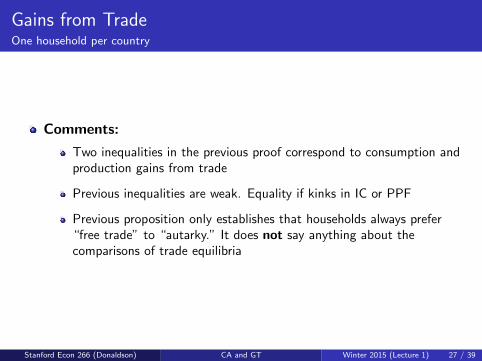
Comments:
Two inequalities in the previous proof correspond to consumption andproduction gains from trade
Previous inequalities are weak. Equality if kinks in IC or PPF
Previous proposition only establishes that households always prefer“free trade” to “autarky.” It does not say anything about thecomparisons of trade equilibria
Stanford Econ 266 (Donaldson) CA and GT Winter 2015 (Lecture 1) 27 / 39
Gains from TradeMultiple households per country (I): domestic lump-sum transfers
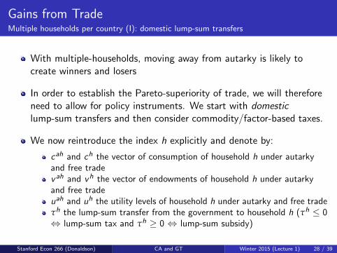
With multiple-households, moving away from autarky is likely tocreate winners and losers
In order to establish the Pareto-superiority of trade, we will thereforeneed to allow for policy instruments. We start with domesticlump-sum transfers and then consider commodity/factor-based taxes.
We now reintroduce the index h explicitly and denote by:
cah and ch the vector of consumption of household h under autarkyand free tradevah and vh the vector of endowments of household h under autarkyand free tradeuah and uh the utility levels of household h under autarky and free tradeτh the lump-sum transfer from the government to household h (τh ≤ 0⇔ lump-sum tax and τh ≥ 0 ⇔ lump-sum subsidy)
Stanford Econ 266 (Donaldson) CA and GT Winter 2015 (Lecture 1) 28 / 39
Gains from TradeMultiple households per country (I): domestic lump-sum transfers
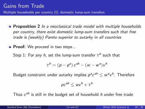
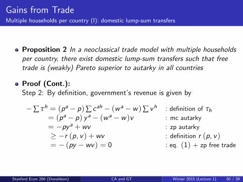
Proposition 2 In a neoclassical trade model with multiple householdsper country, there exist domestic lump-sum transfers such that freetrade is (weakly) Pareto superior to autarky in all countries
Proof: We proceed in two steps...
Step 1: For any h, set the lump-sum transfer τh such that
τh = (p − pa) cah − (w − wa)vh
Budget constraint under autarky implies pacah ≤ wavh. Therefore
pcah ≤ wvh + τh
Thus cah is still in the budget set of household h under free trade
Stanford Econ 266 (Donaldson) CA and GT Winter 2015 (Lecture 1) 29 / 39
Gains from TradeMultiple households per country (I): domestic lump-sum transfers
Proposition 2 In a neoclassical trade model with multiple householdsper country, there exist domestic lump-sum transfers such that freetrade is (weakly) Pareto superior to autarky in all countries
Proof (Cont.):Step 2: By definition, government’s revenue is given by
−∑ τh = (pa − p)∑ cah − (wa − w)∑ vh : definition of τh= (pa − p) ya − (wa − w)v : mc autarky
= −pya + wv : zp autarky
≥ −r (p, v) + wv : definition r (p, v)= − (py − wv) = 0 : eq. (1) + zp free trade
Stanford Econ 266 (Donaldson) CA and GT Winter 2015 (Lecture 1) 30 / 39
Gains from TradeMultiple households per country (I): domestic lump-sum transfers
Comments:
Good to know we don’t need international lump-sum transfersBut these domestic lump-sum transfers remain informationally intensive(cah?)
Stanford Econ 266 (Donaldson) CA and GT Winter 2015 (Lecture 1) 31 / 39
Gains from TradeMultiple households per country (II): commodity and factor taxation
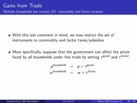
With this last comment in mind, we now restrict the set ofinstruments to commodity and factor taxes/subsidies
More specifically, suppose that the government can affect the pricesfaced by all households under free trade by setting τgood and τfactor
phousehold = p + τgood
whousehold = w + τfactor
Stanford Econ 266 (Donaldson) CA and GT Winter 2015 (Lecture 1) 32 / 39
Gains from TradeMultiple households per country (II): commodity and factor taxation
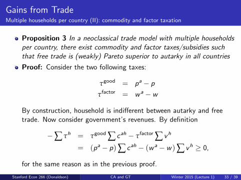
Proposition 3 In a neoclassical trade model with multiple householdsper country, there exist commodity and factor taxes/subsidies suchthat free trade is (weakly) Pareto superior to autarky in all countries
Proof: Consider the two following taxes:
τgood = pa − p
τfactor = wa − w
By construction, household is indifferent between autarky and freetrade. Now consider government’s revenues. By definition
−∑ τh = τgood ∑ cah − τfactor ∑ vh
= (pa − p)∑ cah − (wa − w)∑ vh ≥ 0,
for the same reason as in the previous proof.
Stanford Econ 266 (Donaldson) CA and GT Winter 2015 (Lecture 1) 33 / 39
Gains from TradeMultiple households per country (II): commodity and factor taxation
Comments:
Previous argument only relies on the existence of production gains fromtrade
If there is a kink in the PPF, we know that there aren’t any...
Factor taxation still informationally intensive: need to knowendowments in efficiency units, may lead to different taxes across firms
Stanford Econ 266 (Donaldson) CA and GT Winter 2015 (Lecture 1) 34 / 39
Today’s Plan
1 Course logistics
2 A Brief History of the Field
3 Neoclassical Trade: Standard Assumptions
4 Neoclassical Trade: General Results
1 Gains from Trade2 Law of Comparative Advantage
Stanford Econ 266 (Donaldson) CA and GT Winter 2015 (Lecture 1) 35 / 39
Law of Comparative AdvantageBasic Idea
The previous results have focused on normative predictions
We now demonstrate how the same revealed preference argument canbe used to make positive predictions about the pattern of trade
Principle of comparative advantage:Comparative advantage—meaning differences in relative autarkyprices—is the basis for trade
Why? If two countries have the same autarky prices, then afteropening up to trade, the autarky prices remain equilibrium prices. Sothere will be no trade....
The law of comparative advantage (in words):Countries tend to export goods in which they have a CA, i.e. lowerrelative autarky prices compared to other countries
Stanford Econ 266 (Donaldson) CA and GT Winter 2015 (Lecture 1) 36 / 39
Law of Comparative AdvantageDixit and Norman (1980), Deardorff (1980)
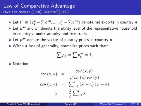
Let tn ≡(yn1 −∑ cnh, ..., ynG −∑ cnh
)denote net exports in country n
Let uan and un denote the utility level of the representative householdin country n under autarky and free trade
Let pan denote the vector of autarky prices in country n
Without loss of generality, normalize prices such that:
∑ pg = ∑ pang = 1,
Notation:
cor (x , y) =cov (x , y)√var (x) var (y)
cov (x , y) = ∑n
i=1(xi − x) (yi − y)
x =1
n ∑n
i=1xi
Stanford Econ 266 (Donaldson) CA and GT Winter 2015 (Lecture 1) 37 / 39
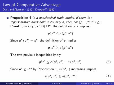
Law of Comparative AdvantageDixit and Norman (1980), Deardorff (1980)
Proposition 4 In a neoclassical trade model, if there is arepresentative household in country n, then cor (p − pa, tn) ≥ 0Proof: Since (yn, vn) ∈ Ωn, the definition of r implies
payn ≤ r (pa, vn)
Since un (cn) = un, the definition of e implies
pacn ≥ e (pa, un)
The two previous inequalities imply
patn ≤ r (pa, vn)− e (pa, un) (3)
Since un ≥ uan by Proposition 1, e (pa, ·) increasing implies
e(pa, un) ≥ e(pa, una) (4)
Stanford Econ 266 (Donaldson) CA and GT Winter 2015 (Lecture 1) 38 / 39
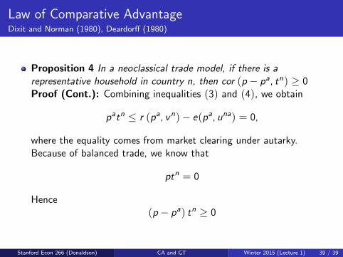
Law of Comparative AdvantageDixit and Norman (1980), Deardorff (1980)
Proposition 4 In a neoclassical trade model, if there is arepresentative household in country n, then cor (p − pa, tn) ≥ 0Proof (Cont.): Combining inequalities (3) and (4), we obtain
patn ≤ r (pa, vn)− e(pa, una) = 0,
where the equality comes from market clearing under autarky.Because of balanced trade, we know that
ptn = 0
Hence(p − pa) tn ≥ 0
Stanford Econ 266 (Donaldson) CA and GT Winter 2015 (Lecture 1) 39 / 39
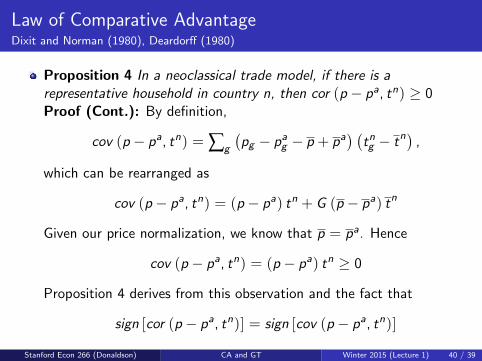
Law of Comparative AdvantageDixit and Norman (1980), Deardorff (1980)
Proposition 4 In a neoclassical trade model, if there is arepresentative household in country n, then cor (p − pa, tn) ≥ 0Proof (Cont.): By definition,
cov (p − pa, tn) = ∑g
(pg − pag − p + pa
) (tng − tn
),
which can be rearranged as
cov (p − pa, tn) = (p − pa) tn + G (p − pa) tn
Given our price normalization, we know that p = pa. Hence
cov (p − pa, tn) = (p − pa) tn ≥ 0
Proposition 4 derives from this observation and the fact that
sign [cor (p − pa, tn)] = sign [cov (p − pa, tn)]
Stanford Econ 266 (Donaldson) CA and GT Winter 2015 (Lecture 1) 40 / 39
Law of Comparative AdvantageDixit and Norman (1980), Deardorff (1980)
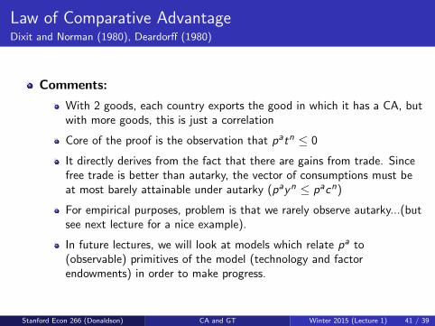
Comments:
With 2 goods, each country exports the good in which it has a CA, butwith more goods, this is just a correlation
Core of the proof is the observation that patn ≤ 0
It directly derives from the fact that there are gains from trade. Sincefree trade is better than autarky, the vector of consumptions must beat most barely attainable under autarky (payn ≤ pacn)
For empirical purposes, problem is that we rarely observe autarky...(butsee next lecture for a nice example).
In future lectures, we will look at models which relate pa to(observable) primitives of the model (technology and factorendowments) in order to make progress.
Stanford Econ 266 (Donaldson) CA and GT Winter 2015 (Lecture 1) 41 / 39