Stochastic Stackelberg equilibria with applications to time-dependentnewsvendor models

Bernt Øksendala,1,∗, Leif Sandalb,2, Jan Ubøeb

aDepartment of Mathematics, University of Oslo, P.O. Box 1053 Blindern, 0316 Oslo, NorwaybNorwegian School of Economics, Helleveien 30, 5045 Bergen, Norway

Abstract

In this paper, we prove a maximum principle for general stochastic differential Stackelberg games, and

apply the theory to continuous time newsvendor problems. In the newsvendor problem, a manufacturer

sells goods to a retailer, and the objective of both parties is to maximize expected profits under a random

demand rate. Our demand rate is an Ito–Levy process, and to increase realism information is delayed,

e.g., due to production time. A special feature of our time-continuous model is that it allows for a

price-dependent demand, thereby opening for strategies where pricing is used to manipulate the demand.

Keywords: stochastic differential games, delayed information, Ito-Levy processes, Stackelberg

equilibria, newsvendor models, optimal control of forward-backward stochastic differential equations

∗Corresponding authorEmail addresses: oksendal@math.uio.no (Bernt Øksendal), leif.sandal@nhh.no (Leif Sandal), jan.uboe@nhh.no (Jan

Ubøe)1The research leading to these results has received funding from the European Research Council under the European

Community’s Seventh Framework Programme (FP7/2007-2013) / ERC grant agreement no [228087]2The research leading to these results has received funding from NFR project 196433

Preprint submitted to Elsevier February 22, 2013

Main variables:

w = wholesale price per unit (chosen by the manufacturer)

q = order quantity (rate chosen by the retailer)

R = retail price per unit (chosen by the retailer)

D = demand (random rate)

M = production cost per unit (fixed)

S = salvage price per unit (fixed)

1. Introduction

The one-period newsvendor model is a widely studied object that has attracted increasing interest in

the last two decades. The basic setting is that a retailer wants to order a quantity q from a manufacturer.

Demand D is a random variable, and the retailer wishes to select an order quantity q maximizing his

expected profit. When the distribution of D is known, this problem is easily solved. The basic problem is

very simple, but appears to have a never-ending number of variations. There is now a very large literature

on such problems, and for further reading we refer to the survey papers by Cachon (2003) and Qin et al.

(2011) and the numerous references therein.

The (discrete) multiperiod newsvendor problem has been studied in detail by many authors, including

Matsuyama (2004), Berling (2006), Bensoussan et al. (2007, 2009), Wang et al., (2010), just to quote

some of the more recent contributions. Two papers whose approach is not unlike that used in our paper

are Kogan (2003) and Kogan and Lou (2003), where the authors consider continuous time-scheduling

problems.

In many cases, demand is not known and the parties gain information through a sequence of obser-

vations. There is a huge literature on cases with partial information, e.g., Scarf (1958), Gallego & Moon

(1993), Bensoussan et al. (2007), Perakis & Roels (2008), Wang et al. (2010), just to mention a few.

When a sufficiently large number of observations have been made, the distribution of demand is fully

revealed and can be used to optimize order quantities. This approach only works if the distribution of D

is static, and leads to false conclusions if demand changes systematically over time. In this paper we will

assume that the demand rate is a stochastic process Dt and we seek optimal decision rules for that case.

In our paper, a retailer and a manufacturer write contracts for a specific delivery rate following a de-

2

cision process in which the manufacturer is the leader who initially decides the wholesale price. Based on

that wholesale price, the retailer decides on the delivery rate and the retail price. We assume a Stackelberg

framework, and hence ignore cases where the retailer can negotiate the wholesale price. The contract is

written at time t−δ, and goods are received at time t. It is essential to assume that information is delayed.

If there is no delay, the demand rate is known, and the retailer’s order rate is made equal to the demand

rate. Information is delayed by a time δ. One justification for this is that production takes time, and

orders cannot be placed and effectuated instantly. It is natural to think about δ as a production lead time.

The single period newsvendor problem with price dependent demand is classical, see Whitin (1955).

Mills (1959) refined the construction considering the case where demand uncertainty is added to the

price-demand curve, while Karlin and Carr (1962) considered the case where demand uncertainty is

multiplied with the price-demand curve. For a nice review of the problem with extensions see Petruzzi

and Dada (1999). Stackelberg games for single period newsvendor problems with fixed retail price have

been studied extensively by Lariviere and Porteus (2001), providing quite general conditions under which

unique equilibria can be found.

Multiperiod newsvendor problems with delayed information have been discussed in several papers, but

none of these papers appears to make the theory operational. Bensoussan et al. (2009) use a time-discrete

approach and generalize several information delay models. However, these are all under the assumption

of independence of the delay process from inventory, demand, and the ordering process. They assert that

removing this assumption would give rise to interesting as well as challenging research problems, and

that a study of computation of the optimal base stock levels and their behavior with respect to problem

parameters would be of interest. Computational issues are not explored in their paper, and they only

consider decision problems for inventory managers, disregarding any game theoretical issues.

Calzolari et al. (2011) discuss filtering of stochastic systems with fixed delay, indicating that problems

with delay lead to nontrivial numerical difficulties even when the driving process is Brownian motion. In

our paper, solutions to general delayed newsvendor equilibria are formulated in terms of coupled systems

of stochastic differential equations. Our approach may hence be useful also in the general case where

closed form solutions cannot be obtained.

Stochastic differential games have been studied extensively in the literature. However, most of the

works in this area have been based on dynamic programming and the associated Hamilon-Jacobi-Bellman-

Isaacs type of equations for systems driven by Brownian motion only. More recently, papers on stochastic

3

differential games based on the maximum principle (including jump diffusions) have appeared. See, e.g.,

Øksendal and Sulem (2012) and the references therein. This is the approach used in our paper, and as

far as we know, the application to the newsvendor model is new. The advantage with the maximum

approach is two-fold:

• We can handle non-Markovian state equations and non-Markovian payoffs.

• We can deal with games with partial and asymmetric information.

Figure 1 shows a sample path of an Ornstein–Uhlenbeck process that is mean reverting around a level

µ = 100. Even though the long-time average is 100, orders based on this average are clearly suboptimal.

At, e.g., t = 30, we observe a demand rate D30 = 157. When the mean reversion rate is as slow as

in Figure 1, the information D30 = 157 increases the odds that the demand rate is more than 100 at

time t = 37. If the delay δ = 7 (days), the retailer should hence try to exploit this extra information to

improve performance.

δ

0 50 100 150 200 t

50

100

150

200

Dt

Figure 1: An Ornstein–Uhlenbeck process with delayed information

Based on the information available at time t − δ, the manufacturer should offer the retailer a price

per unit wt for items delivered at time t. Given the wholesale price wt and all available information, the

retailer should decide on an order rate qt and a retail price Rt. The retail price can in principle lead to

changes in demand, and in general the demand rate Dt is, hence, a function of Rt. However, such cases

are hard to solve in terms of explicit expressions. We will also look at the simplified case where R is

exogenously given and fixed. To carry out our construction, we will need to assume that items cannot

be stored. That is of course a strong limitation, but applies to important cases like electricity markets

and markets for fresh foods.

4

Assuming that both parties have full information about demand rate at time t− δ, and that the man-

ufacturer knows how much the retailer will order at any given unit price w, we are left with a Stackelberg

game where the manufacturer is the leader and the retailer is the follower. To our knowledge, stochastic

differential games of this sort have not been discussed in the literature previously. Before we can discuss

game equilibria for the newsvendor problem, we must formulate and prove a maximum principle for

general stochastic differential Stackelberg games.

In the case where R is exogenously given and fixed, it seems reasonable to conjecture that our op-

timization problem could be reduced to solving a family of static newsvendor problems pointwise in t.

Theorem 3.2.2 confirms that this approach provides the correct solution to the problem. Note, however,

that our general framework is non-Markovian, and that solutions may depend on path properties of the

demand.

The paper is organized as follows. In Section 2, we set up a framework where we discuss general

stochastic differential Stackelberg games. In Section 3, we use the machinery in Section 2 to consider a

continuous-time newsvendor problem. In Section 4, we consider the special case where the demand rate

is given by an Ornstein–Uhlenbeck process and provide explicit solutions for the unique equilibria that

occur in that case. Examples with R-dependent demand are considered in Section 5. Finally, in Section

6 we offer some concluding remarks.

2. General stochastic differential Stackelberg games

In this section, we will consider general stochastic differential Stackelberg games. In our framework,

the state of the system is given by a stochastic process Xt. The game has two players. Player 1 (leader,

denoted by L) can at time t choose a control uL(t) while player 2 (follower, denoted by F ) can choose a

control uF (t). The controls determine how Xt evolves in time. The performance for player i is assumed

to be of the form

Ji(uL, uF ) = E

[∫ T

δ

fi(t,Xt, uL(t), uF (t), ω)dt+ gi(XT , ω)

]i = L,F (1)

where fi(t, x, w, v, ω) : [0, T ]×R×Rl×Rm×Ω→ R is a given Ft-adapted process and gi(x, ω) : R×Ω→ R

are given FT -measurable random variables for each x,w, v; i = L,F . We will assume that fi are C1 in

v, w, x and that gi are C1 in x, i = L,F .

5

In our Stackelberg game, player 1 is the leader, and player 2 the follower. Hence when uL is revealed

to the follower, the follower will choose uF to maximize JF (uL, uF ). The leader knows that the follower

will act in this rational way.

Suppose that for any given control uL there exists a map Φ (a “maximizer” map) that selects uF that

maximizes JF (uL, uF ). The leader will hence choose uL = u∗L such that uL 7→ JL(uL,Φ(uL)) is maximal

for uL = u∗L. In order to solve problems of this type we need to specify how the state of the system

evolves in time. We will assume that the state of the system is given by a controlled jump diffusion of

the form:

dXt = µ(t,Xt, u(t), ω)dt+ σ(t,Xt, u(t), ω)dBt

+∫

Rγ(t,Xt− , u(t), ξ, ω)N(dt, dξ) (2)

X(0) = x ∈ R

where the coefficients µ(t, x, u, ω) : [0, T ]× R× U× Ω → R, σ(t, x, u, ω) : [0, T ]× R× U× Ω → R× Rn,

γ(t, x, u, ξ, ω) : [0, T ]× R× U× R0 × Ω→ R are given continuous functions assumed to be continuously

differentiable with respect to x and u, and R0 = R \ 0. Here Bt = B(t, ω); (t, ω) ∈ [0,∞) × Ω is a

Brownian motion in Rn and N(dt, dξ) = N(dt, dξ, ω) is an independent compensated Poisson random

measure on a filtered probability space (Ω,F , Ftt≥0, P ). See Øksendal and Sulem (2007) for more

information about controlled jump diffusions. The set U = UL × UF is a given set of admissible control

values u(t, ω). We assume that the control u = u(t, ω) consists of two components, u = (uL, uF ), where

the leader controls uL∈ Rl and the follower controls uF∈ Rm. We also assume that the information flow

available to the players is given by the filtration Ett∈[0,T ], where

Et ⊆ Ft for all t ∈ [0, T ]. (3)

For example, the case much studied in this paper is when

Et = Ft−δ for all t ∈ [δ, T ]. (4)

for some fixed information delay δ > 0. We assume that uL(t) and uF (t) are Et-predictable, and assume

there is given a family AE= AL,E ×AF,E of admissible controls contained in the set of Et-predictable

processes.

6

We now consider the following game theoretic situation:

Suppose the leader decides her control process uL ∈ AL,E . At any time t the value is immediately

known to the follower. Therefore he chooses uF = u∗F ∈ AF,E such that

uF 7→ JF (uL, uF ) is maximal for uF = u∗F . (5)

Assume that there exists a measurable map Φ : AL,E → AF,E such that

uF 7→ JF (uL, uF ) is maximal for uF = u∗F = Φ(uL) (6)

The leader knows that the follower will act in this rational way. Therefore the leader will choose uL =

u∗L ∈ AL,E such that

uL 7→ JL(uL,Φ(uL)) is maximal for uL = u∗L. (7)

The control u∗ := (u∗L,Φ(u∗L)) ∈ AL,E ×AF,E is called a Stackelberg equilibrium for the game defined by

(1)-(2). In the newsvendor problem studied in this paper, the leader is the manufacturer who decides the

wholesale price uL = w for the retailer, who is the follower, and who decides the order rate u(1)F = q and

the retailer price u(2)F = R. Thus uF = (q,R). We may summarize (5) and (7) as follows:

maxuF∈AF,E

JF (uL, uF ) = JF (uL,Φ(uL)) (8)

and

maxuL∈AL,E

JL(uL,Φ(uL)) = JL(u∗L,Φ(u∗L)) (9)

We see that (8) and (9) constitute two consecutive stochastic control problems with partial informa-

tion, and hence we can, under some conditions, use the maximum principle for such problems as pre-

sented in Øksendal and Sulem (2012) (see also, e.g., Framstad et al. (2004) and Baghery and Øksendal

(2007)) to find a maximum principle for Stackelberg equilibria. To this end, we define the Hamiltonian

HF (t, x, u, aF , bF , cF (·), ω) : [0, T ]× R× U× R× Rn+1 ×R×Ω→ R by

HF (t, x, u, aF , bF , cF (·), ω) = fF (t, x, u, ω) + µ(t, x, u, ω)aF + σ(t, x, u, ω)bF (10)

+∫

Rγ(t, x, u, ξ, ω)cF (ξ)ν(dξ);

where R is the set of functions c(·) : R0 → R such that (10) converges, ν is a Levy measure. For simplicity

7

of notation the explicit dependence on ω ∈ Ω is suppressed in the following. The adjoint equation for HF

in the unknown adjoint processes aF (t), bF (t), and cF (t, ξ) is the following backward stochastic differential

equation (BSDE):

daF (t) = −∂HF

∂x(t,X(t), u(t), aF (t), bF (t), cF (t, ·))dt (11)

+ bF (t)dBt +∫

RcF (t, ξ)N(dt, dξ); 0 ≤ t ≤ T

aF (T ) = gF′(X(T )) (12)

Here X(t) = Xu(t) is the solution to (2) corresponding to the control u ∈ AE . Next, assume that there

exists a function φ : [0, T ]× UL × Ω→ UF such that

Φ(uL)(t) = φ(t, ul(t)) i.e Φ(uL) = φ(·, uL(·)) (13)

Define the Hamiltonian HφL(t, x, uL, aL, bL, cL(·)) : [0, T ]× R× UL × R× Rn+1 ×R → R by

HφL(t, x, uL, aL, bL, cL(·)) = fL(t, x, uL,Φ(uL)) + µ(t, x, uL,Φ(uL))aL (14)

+ σ(t, x, uL,Φ(uL))bL +∫

Rγ(t, x, uL,Φ(uL), ξ)cL(ξ)ν(dξ)

The adjoint equation (for HφL) in the unknown processes aL(t), bL(t), cL(t, ξ) is the following BSDE:

daL(t) = −∂Hφ

L

∂x(t,X(t), uL(t), φ(t, uL(t)), aL(t), bL(t), cL(t, ·))dt (15)

+ bL(t)dBt +∫

RcL(t, ξ)N(dt, dξ); 0 ≤ t ≤ T

aL(T ) = gL′(X(T )) (16)

Here X(t) = XuL,Φ(uL)(t) is the solution to (2) corresponding to the control u(t) := (uL(t), φ(t, uL(t)));

t ∈ [0, T ], assuming that this is admissible.

We make the following assumptions:

(A1) For all ui ∈ Ai,E and all bounded βi ∈ Ai,E there exists ε > 0 such that

ui + sβi ∈ Ai,E for all s ∈ (−ε, ε); i = L,F .

8

(A2) For all t0 ∈ [0, T ] and all bounded Et0-measurable random variables αi, the control process

βi(t) defined by

βi(t) =

αi if t ∈ [t0, T ]

0 otherwise; t ∈ [0, T ]

belongs to Ai,E ; i = L,F .

(A3) For all ui, βi ∈ Ai,E with βi bounded, the derivative processes

ξL(t) =d

ds

(XuL+sβL,uF (t)

) ∣∣∣s=0

ξF (t) =d

ds

(XuL,uF+sβF (t)

) ∣∣∣s=0

exist and belong to L2(λ× P ), where λ denotes Lebesgue measure on [0, T ].

We can now formulate our maximum principle for Stackelberg equilibria:

Theorem 2.1 (Maximum principle)

Assume that (13) and (A1)–(A3) hold. Put u = (uL, uF ) = (uL,Φ(uL)) where Φ : UL → UF , and let

X(t), (ai, bi, ci) be the corresponding solutions of (2), (11)–(12) (for i = F ) and (15)–(16) (for i = L),

respectively.

Suppose that for all bounded βi ∈ Ai,E , i = L,F we have

E[ ∫ T

0

(ai(t))2

((∂σ∂x

(t)ξi(i) +∂σ

∂ui(t)βi(t)

)2

+∫

R

(∂γ∂x

(t, ζ)ξi(t) +∂γ

∂ui(t, ζ)βi(t)

)2

ν(dζ))

(17)

+ ξ2i (t)

((bi(t))2 +

∫R

(ci(t, ζ))2ν(dζ))

dt

]<∞

Then the following, (I) and (II), are equivalent.

(I)d

ds(JF (uL,Φ(uL) + sβF ))

∣∣s=0

=d

ds(JL(uL + sβL,Φ(uL + sβL)))

∣∣s=0

= 0 (18)

for all bounded βL ∈ AL,E , βF ∈ AF,E .

(II)

E[∂

∂vFHF (t,X(t), uL(t), vF , aF (t), bF (t), cF (t, ·))

∣∣∣∣Et]vF=Φ(uL)

= 0 (19)

for j = 1, 2 and

9

E[∂

∂vLHφL(t,X(t), vL, aL(t), bL(t), cL(t, ·))

∣∣∣∣Et]vL=uL(t)

= 0 (20)

Proof

This follows by first applying the maximum principle for optimal control with respect to uF ∈ AF,E of

the state process XuL,uF (t) for fixed uL ∈ AL,E , as presented in Øksendal and Sulem (2012). See also

Framstad et al. (2004), Baghery and Øksendal (2007), Øksendal and Sulem (2007). Next we apply the

same maximum principle with respect to uL ∈ AL,E of the state process XuL,Φ(uL)(t), for the given

function Φ. We omit the details.

Corollary 2.2

Suppose (uL,Φ(uL)) is a Stackelberg equilibrium for the game (1)-(2) and that (13), (A1)-(A3), and (17)

are satisfied. Then the first order conditions (19)–(20) hold.

3. A continuous time newsvendor problem

In this section, we will formulate a continuous time newsvendor problem and use the results in Sec-

tion 2 to describe a set of explicit equations that we need to solve to find Stackelberg equilibria. We

will assume that the demand rate for a good is given by a (possibly controlled) stochastic process Dt. A

retailer is at time t− δ offered a unit price wt for items to be delivered at time t. Here δ > 0 is the delay

time. At time t− δ, the retailer chooses an order rate qt. The retailer also decides a retail price Rt. We

assume that items can be salvaged at a unit price S ≥ 0, and that items cannot be stored, i.e., they must

be sold instantly or salvaged.

Remarks

The delay δ can be interpreted as a production lead time, and it is natural to assume that wt and qt

should both be settled at time t − δ. In general the retail price Rt can be settled at a later stage. To

simplify notation we assume that Rt, too, is settled at time t− δ. The assumption that items cannot be

stored is, of course, quite restrictive. Many important cases lead to assumptions of this kind; we mention

in particular the electricity market and markets for fresh foods.

Assuming that sale will take part in the time period δ ≤ t ≤ T , the retailer will get an expected profit

10

JF (w, q,R) = E

[∫ T

δ

(Rt − S) min[Dt, qt]− (wt − S)qtdt

](21)

When the manufacturer has a fixed production cost per unit M , the manufacturer will get an expected

profit

JL(w, q,R) = E

[∫ T

δ

(wt −M)qtdt

](22)

Technical remarks

To solve these problems mathematically, it is convenient to apply an equivalent mathematical formulation:

At time t the retailer orders the quantity t for immediate delivery, but the information at that time is the

delayed information Ft−δ about the demand δ units of time. Similarly, when the manufacturer delivers

the ordered quantity qt at time t, the unit price wt is based on Ft−δ. From a practical point of view this

formulation is entirely different, but leads to the same optimization problem.

3.1. Formalized information

We will assume that our demand rate is given by a (possibly controlled) process of the form

dDt = µ(t,Dt, Rt, ω)dt+ σ(t,Dt, Rt, ω)dBt +∫

Rγ(t,Dt− , Rt, ξ, ω)N(dt, dξ); t ∈ [0, T ] (23)

D0 = d0 ∈ R

Brownian motion Bt and the compensated Poisson term N(t, dz) are driving the stochastic differential

equation in (23), and it is hence natural to formalize information with respect to these objects. We

therefore let Ft denote the σ-algebra generated by Bs and N(s, dz), 0 ≤ s ≤ t. Intuitively Ft contains

all the information up to time t. When information is delayed, we instead consider the σ-algebras

Et := Ft−δ t ∈ [δ, T ] (24)

Both the retailer and the manufacturer should base their actions on the delayed information. Technically

that means that qt and wt should be Et-adapted, i.e., q and w should be E-predictable processes. In

principle, the retail price Rt can be settled at a later stage. This case is possible to handle, but leads to

complicated notation. We hence only consider the case where Rt is E-predictable.

11

3.2. Finding Stackelberg equilibria in the newsvendor model

We now apply our general result for stochastic Stackelberg games to the newsvendor problem. In

the newsvendor problem, we have the control u = (uL, uF ) where uL = w is the wholesale price, and

uF = (q,R) with q the order rate and R the retail price. Moreover Xt = Dt,

fL(t,X(t), u(t)) = (wt −M)qt, gL = 0, (25)

fF (t,X(t), u(t)) = (Rt − S) min(Dt, qt)− (wt − S)qt, and gF = 0. (26)

Therefore by (10)

HF (t,Dt, qt, Rt, wt, aF (t), bF (t), cF (t, ·)) = (Rt − S) min(Dt, qt)− (wt − S)qt (27)

+ aF (t)µ(t,Dt, Rt) + bF (t)σ(t,Dt, Rt)

+∫

Rγ(t,Dt, Rt, ξ)cF (ξ)ν(dξ)

Similarly by (14) , with uF = φ(uL) = (φ1(w), φ2(w)) = (q(w), R(w)),

HφL(t,Dt, wt, aL(t), bL(t), cL(t, ·)) (28)

=(wt −M)φ1(t, w(t)) + aL(t)µ(t,Dt, φ2(t, w(t))) + bL(t)σ(t,Dt, φ2(t, w(t)))) (29)

+∫

RcL(t, ξ)γ(t,Dt, φ2(t, w(t)), ξ)ν(dξ) (30)

Here we have assumed that the dynamics of Dt only depends on the control Rt = φ2(t, w(t)) and has the

general form

dDt = µ(t,Dt, Rt)dt+ σ(t,Dt, Rt)dBt (31)

+∫

Rγ(t,Dt− , Rt, ξ)N(dt, dξ); t ∈ [0, T ]

D0 = d0 ∈ R (32)

where µ(t,D,R), σ(t,D,R) and γ(t,D, T, ξ) are continuous with respect to t and continuously differen-

tiable (C1) with respect to D and R. We chooseAL,E ,AF,E to be the set of all E-predictable processes with

values in UL = R and UF = R2 respectively, where Et = Ft−δ as above. Then we see that assumptions

12

(A1)-(A3) hold, with ξL(t) and ξF (t) given by ξL(t) = 0 for all t ∈ [0, T ] and

dξF (t) = ξF (t)(∂µ

∂D(t,Dt, Rt)dt+

∂σ

∂D(t,Dt, Rt)dBt +

∫R

∂γ

∂D(t,Dt− , Rt, ξ)N(dt, dξ)

)(33)

+ βF (t) ·(∂µ

∂R(t,Dt, Rt)dt+

∂σ

∂R(t,Dt, Rt)dBt +

∫R

∂γ

∂R(t,Dt− , Rt, ξ)N(dt, dξ)

); t ∈ [0, T ]

ξF (0) = 0 (34)

where · denotes a vector product. To find a Stackelberg equilibrium we use Theorem 2.1. Hence by (19)

we get the following first order conditions for the optimal values qt = φ1(t, w(t)), Rt = φ2(t, w(t)):

E[(Rt − S)X[0,Dt](qt)− wt + S

∣∣Et] = 0 (35)

and

E[

min(Dt, qt) + aF (t)∂µ

∂R(t,Dt, R) (36)

+bF (t)∂σ

∂R(t,Dt, R) +

∫RcF (t, ξ)

∂γ

∂R(t,Dt, R, ξ)ν(dξ)

∣∣∣Et] = 0

Here X[0,Dt](qt) denotes the indicator function for the interval [0, Dt], i.e., a function that has the value

1 if 0 ≤ qt ≤ Dt, and is zero otherwise. Let qt = Φ1(w)(t), Rt = Φ2(w)(t) be the solution of this coupled

system. Next, by (20) we get the first-order condition

(wt −M)φ′1(t, w(t)) + φ1(t, w(t)) + φ′2(t, w(t))E[aL(t)

∂µ

∂R(t,Dtφ2(t, w(t))) (37)

+bL(t)∂σ

∂R(t,Dt, φ2(t, w(t))) +

∫RcL(t, ξ)

∂γ

∂R(t,Dt, φ2(t, w(t)), ξ)ν(dξ)

∣∣∣Et] = 0

for the optimal value wt. We summarize what we have proved in the following theorem.

Theorem 3.2.1

Suppose u∗ is a Stackelberg equilibrium for the newsvendor problem with state Xt = Dt given by (31) and

performance functionals

JL(w, (q,R)) = E

[∫ T

δ

(wt −M)qtdt

](manufacturer’s profit) (38)

JF (w, (q,R)) = E

[∫ T

δ

((Rt − S) min(Dt, qt)− (wt − S)qt

)dt

](retailer’s profit) (39)

13

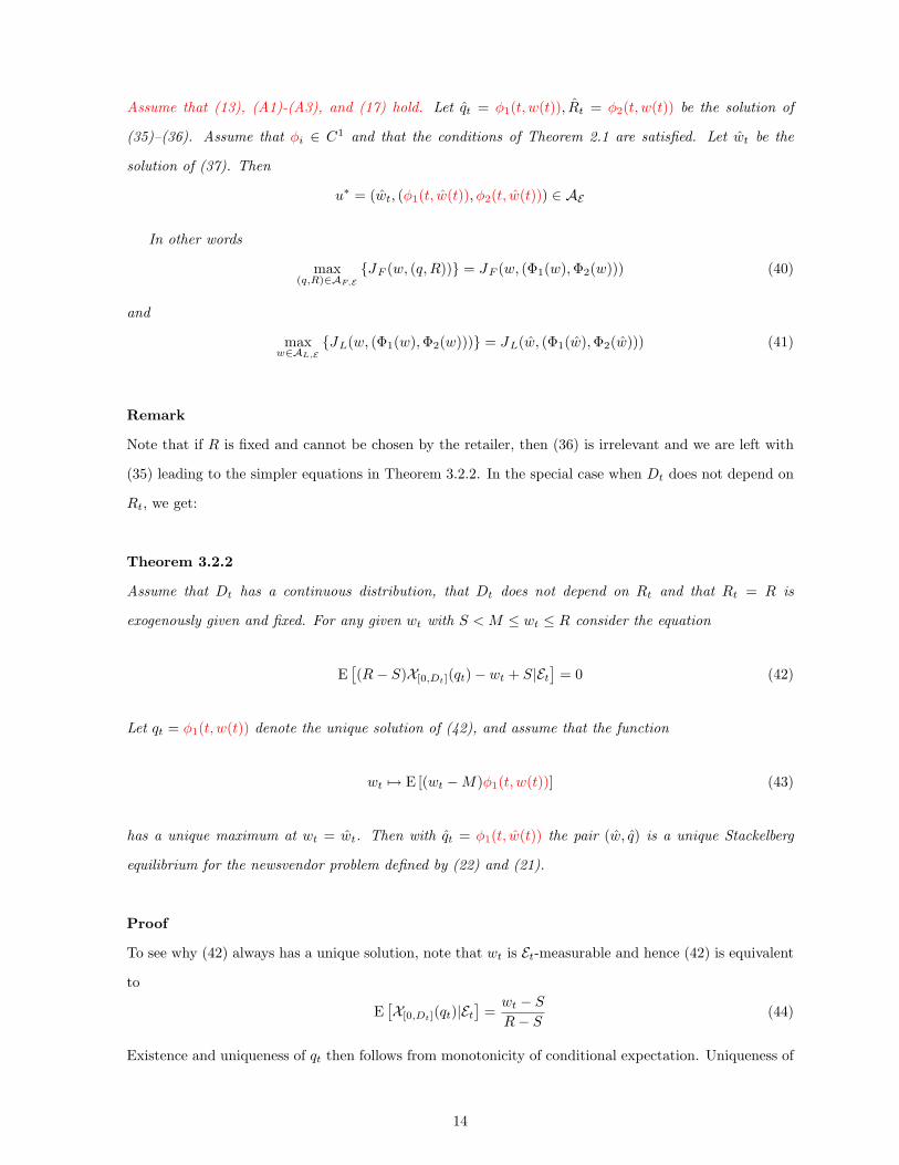
Assume that (13), (A1)-(A3), and (17) hold. Let qt = φ1(t, w(t)), Rt = φ2(t, w(t)) be the solution of

(35)–(36). Assume that φi ∈ C1 and that the conditions of Theorem 2.1 are satisfied. Let wt be the

solution of (37). Then

u∗ = (wt, (φ1(t, w(t)), φ2(t, w(t))) ∈ AE

In other words

max(q,R)∈AF,E

JF (w, (q,R)) = JF (w, (Φ1(w),Φ2(w))) (40)

and

maxw∈AL,E

JL(w, (Φ1(w),Φ2(w))) = JL(w, (Φ1(w),Φ2(w))) (41)

Remark

Note that if R is fixed and cannot be chosen by the retailer, then (36) is irrelevant and we are left with

(35) leading to the simpler equations in Theorem 3.2.2. In the special case when Dt does not depend on

Rt, we get:

Theorem 3.2.2

Assume that Dt has a continuous distribution, that Dt does not depend on Rt and that Rt = R is

exogenously given and fixed. For any given wt with S < M ≤ wt ≤ R consider the equation

E[(R− S)X[0,Dt](qt)− wt + S|Et

]= 0 (42)

Let qt = φ1(t, w(t)) denote the unique solution of (42), and assume that the function

wt 7→ E [(wt −M)φ1(t, w(t))] (43)

has a unique maximum at wt = wt. Then with qt = φ1(t, w(t)) the pair (w, q) is a unique Stackelberg

equilibrium for the newsvendor problem defined by (22) and (21).

Proof

To see why (42) always has a unique solution, note that wt is Et-measurable and hence (42) is equivalent

to

E[X[0,Dt](qt)|Et

]=wt − SR− S

(44)

Existence and uniqueness of qt then follows from monotonicity of conditional expectation. Uniqueness of

14

the Stackelberg equilibrium follows from Theorem 3.2.1. To see that the candidate qt = Φ1(w)(t) is indeed

a Stackelberg Equilibrium, we argue as follows: Since the maximum wt is unique, any other wt will lead

to strictly lower expected profit at time t. As demand does not depend on wt, low expected profit at one

point in time cannot be compensated by higher expected profits later on. Hence if the statement wt = wt

a.s. λ × P (λ denotes Lebesgue measure on [0, T ]) is false, any such strategy will lead to strictly lower

expected profits. The same argument applies for the retailer, and hence (w, q) is a Stackelberg equilibrium.

To avoid degenerate cases we need to know that Dt has a continuous distribution. In the next sec-

tions we will consider special cases, and we will often be able to write down explicit solutions to (42) and

prove that (43) has a unique maximum. Notice that (42) is an equation defined in terms of conditional

expectation. Conditional statements of this type are in general difficult to compute, and the challenge is

to state the result in terms of unconditional expectations.

4. Explicit solution formulas

In this section we will assume that the conditions of Theorem 2.1 hold.

4.1. The Ornstein-Uhlenbeck process with constant coefficients

In this section, we offer explicit formulas for the equilibria that occur when the demand rate is given

by a constant coefficient Ornstein–Uhlenbeck process, i.e., the case where Dt is given by

dDt = a(µ−Dt)dt+ σdBt (45)

where a, µ, and σ are constants. The Ornstein–Uhlenbeck process is important in many applications.

In particular, it is commonly used as a model for the electricity market. The process is mean reverting

around the constant level µ, and the constant a decides the speed of mean reversion. The explicit solution

to (45) is

Dt = D0e−at + µ(1− e−at) +

∫ t

0

σea(s−t)dBs (46)

It is easy to see that

Dt = Dt−δe−aδ + µ(1− e−aδ) +

∫ t

t−δσea(s−t)dBs (47)

15

Because the last term is independent of Et with a normal distribution N(0, σ2(1−e−2aδ)

2a ), it is easy to

find a closed form solution to (42). We let G[z] denote the cumulative distribution of a standard normal

distribution, and G−1[z] its inverse. The final result can be stated as follows:

Proposition 4.1.1

For each y ∈ R, let Φy : [M,R]→ R denote the function

Φy[w] = ye−aδ + µ(1− e−aδ) + σ

√1− e−2aδ

2a·G−1

[1− w − S

R− S

](48)

and let Ψy : [M,R] → R denote the function Ψy[w] = (w −M)Φy[w]. If Φy[M ] > 0, the function Ψy is

quasiconcave and has a unique maximum with a strictly positive function value.

At time t− δ the parties should observe y = Dt−δ, and a unique Stackelberg equilibrium is obtained

at

w∗t =

Argmax[Ψy] if Φy[M ] > 0

M otherwiseq∗t =

Φy[Argmax[Ψy]] if Φy[M ] > 0

0 otherwise(49)

To prove Proposition 4.1.1, we need the following lemma.

Lemma 4.1.2

In this lemma G[x] is the cumulative distribution function of the standard normal distribution. Let

0 ≤ m ≤ 1, and for each m consider the function hm : R→ R defined by

hm[z] = z(1−m−G[z])−G′[z] (50)

Then

hm[z] < 0 for all z ∈ R (51)

Proof of Lemma 4.1.2

Note that if z ≥ 0, then hm[z] ≤ h0[z] and if z ≤ 0, then hm[z] ≤ hL[z]. It hence suffices to prove the

lemma for m = 0 and m = 1. Using G′′[z] = −z · G′[z], it is easy to see that h′′m[z] = −G′[z] ≤ 0. If

m = 0, it is straightforward to check that h0 is strictly increasing, and that limz→+∞ h0[z] = 0. If m = 1,

it is straightforward to check that hL[z] is strictly decreasing, and that limz→−∞ hL[z] = 0. This proves

that h0 and hL are strictly negative, completing the proof of the lemma.

16

Proof of Proposition 4.1.1

From (47), we easily see that the statement qt ≤ Dt is equivalent to the inequality

qt −(Dt−δe

−aδ + µ(1− e−aδ)≤∫ t

t−δσea(s−t)dBs (52)

The left-hand side is Et-measurable, while the right-hand side is normally distributed and independent

of Et. Using the Ito isometry, we see that the right-hand side has expected value zero and varianceσ2(1−e−2aδ)

2a . It is then straightforward to see that

E[X[0,Dt](qt)|Et

]= 1−G

qt − (Dt−δe−aδ + µ(1− e−aδ)

)√σ2(1−e−2aδ)

2a

(53)

and (48) follows trivially from (44). It remains to prove that the function Ψy has a unique maximum if

Φy[M ] > 0. First put

y =y · e−aδ + µ(1− e−aδ)

σ√

1−e−2aδ

2a

(54)

and note that Ψy is proportional to

(w −M)(y +G−1

[1− w − S

R− S

])(55)

We make a monotone change of variables using z = G−1[1− w−S

R−S

]. With this change of variables we

see that Ψy is proportional to

(R− S)(

1−G[z]− M − SR− S

)(y + z) (56)

Put m = M−SR−S , and note that Ψy is proportional to

(1−m−G[z])(y + z) (57)

Φy[M ] > 0 is equivalent to y+G−1[1−m] > 0, and the condition w ≥M is equivalent to z ≤ G−1[1−m].

Note that if S ≤M ≤ R, then 0 ≤ m ≤ 1. For each fixed 0 ≤ m ≤ 1, y ∈ R consider the function

fm[z] = (1−m−G[z])(y + z) on the interval − y ≤ z ≤ G−1[1−m] (58)

17

If y +G−1[1−m] > 0, the interval is nondegenerate and nonempty, and

f ′m[z] = −G′[z](y + z) + (1−m−G[z]) (59)

Note that f ′m[−y] > 0, and that fm[−y] = fm[G−1[1 −m]] = 0. These functions therefore have at least

one strictly positive maximum. To prove that the maximum is unique, assume that f ′m[z0] = 0, and

compute f ′′m[z0]. Using G′′[z] = −z · g′[z], it follows that

f ′′m[z0] = z0(1−m−G[z0])− 2G′[z0] < z0(1−m−G[z0])−G′[z0] < 0 (60)

by Lemma 4.1.2. The function is thus quasiconcave and has a unique, strictly positive maximum. Exis-

tence of a unique Stackelberg equilibrium then follows from Theorem 3.2.2.

The condition Φy[M ] > 0 has an obvious interpretation. The manufacturer cannot offer a wholesale

price w lower than the production cost M . If Φy[M ] ≤ 0, it means that the retailer is unable to make a

positive expected profit even at the lowest wholesale price the manufacturer can offer. When that occurs,

the retailer’s best strategy is to order q = 0 units. When the retailer orders q = 0 units, the choice of w

is arbitrary. However, the choice w = M is the only strategy that is increasing and continuous in y.

Given values for the parameters a, µ, σ, S,M,R, and δ, the explicit expression in (48) makes it straight-

forward to construct the deterministic function y 7→ Argmax[Ψy] numerically. Two different graphs of

this function are shown in Figure 2. Figure 3 shows the corresponding function Φy[Argmax[Ψy]]. In the

construction we used a delay δ = 7 and δ = 30, with the parameter values

a = 0.05 µ = 100 σ = 12 R = 10 S = 1 M = 2 (61)

50 100 150 200 250Dt-∆

6.0

6.5

7.0

7.5

8.0

8.5

wt*

50 100 150 200 250Dt-∆

5.5

6.0

wt*

δ = 7 δ = 30

Figure 2: w∗t as a function of the observed demand rate D = Dt−δ

18

50 100 150 200 250Dt-∆

60

80

100

120

140

qt*

50 100 150 200 250Dt-∆

140

150

160

170

180

190

qt*

δ = 7 δ = 30

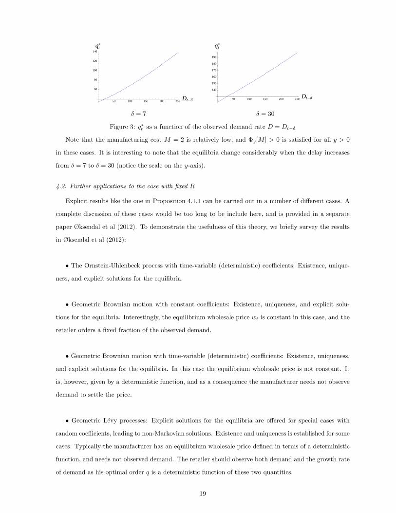
Figure 3: q∗t as a function of the observed demand rate D = Dt−δ

Note that the manufacturing cost M = 2 is relatively low, and Φy[M ] > 0 is satisfied for all y > 0

in these cases. It is interesting to note that the equilibria change considerably when the delay increases

from δ = 7 to δ = 30 (notice the scale on the y-axis).

4.2. Further applications to the case with fixed R

Explicit results like the one in Proposition 4.1.1 can be carried out in a number of different cases. A

complete discussion of these cases would be too long to be include here, and is provided in a separate

paper Øksendal et al (2012). To demonstrate the usefulness of this theory, we briefly survey the results

in Øksendal et al (2012):

• The Ornstein-Uhlenbeck process with time-variable (deterministic) coefficients: Existence, unique-

ness, and explicit solutions for the equilibria.

• Geometric Brownian motion with constant coefficients: Existence, uniqueness, and explicit solu-

tions for the equilibria. Interestingly, the equilibrium wholesale price wt is constant in this case, and the

retailer orders a fixed fraction of the observed demand.

• Geometric Brownian motion with time-variable (deterministic) coefficients: Existence, uniqueness,

and explicit solutions for the equilibria. In this case the equilibrium wholesale price is not constant. It

is, however, given by a deterministic function, and as a consequence the manufacturer needs not observe

demand to settle the price.

• Geometric Levy processes: Explicit solutions for the equilibria are offered for special cases with

random coefficients, leading to non-Markovian solutions. Existence and uniqueness is established for some

cases. Typically the manufacturer has an equilibrium wholesale price defined in terms of a deterministic

function, and needs not observed demand. The retailer should observe both demand and the growth rate

of demand as his optimal order q is a deterministic function of these two quantities.

19

5. R-dependent demand

In this section we provide a solution to an example with R-dependent demand. This problem is more

difficult than the case we handled in the previous section. We also discuss a more complicated example,

raising some interesting issues for future research.

5.1. An example with R-dependent demand

When demand depends on Rt, Theorem 3.2.2 no longer applies. High profits at some stage may

become too costly later, due to reduced demand, and the problem can no longer be separated into

independent one-periodic problems. In particular we shall see that (13) no longer holds. However, we can

still apply the maximum principle for the optimization of JF (the follower problem), since this part does

not need (13). To simplify the discussion, we note that in the particular case where the coefficients µ, σ, γ

do not depend on D, then the adjoint equations (15)–(16) have the trivial solution aL(t) = bL(t) = 0. If

dDt = (K −Rt)dt+ σdBt (62)

the second pair of adjoint variables is also solvable, i.e., (11)–(12) has the explicit solution

aF (t) = E

[∫ T

t

(Rs − S)X[0,qs](Ds)ds|Et

]bF (t) = 0 (63)

If we make the simplifying assumption that Rt is decided at time t−δ, i.e., at the same time as wt and qt,

then, maximizing the Hamiltonian HF as in Theorem 3.2.1, we arrive by (33) and (34) at the following

first-order conditions for the optimal functions wt = wt, q = qt = Φ1(w)(t) and R = Rt = Φ2(w)(t):

E[X[0,D+

t ](qt)|Et]

=wt − SRt − S

t ∈ [δ, T ] (64)

E

[min[Dt, qt]−

∫ T

t

(Rs − S)X[0,qs](Ds)ds|Et

]= 0 t ∈ [δ, T ] (65)

The functions φ1 and φ2 are found solving (64)-(65), as explained in the following.

It is interesting to note that while (64) can be solved pointwise in t, (65) depends on path properties in

the remaining time period, reflecting that decisions taken at one point in time influence later performance.

The optimal order quantity qt = Φ1(w)(t) can be found from the equations as follows: Using the same

separation technique that we used in Section 4, we can express qt explicitly in terms of wt and Rt:

qt = Dt−δ +∫ t

t−δ(K −Rs)ds+

√σδ ·G−1

[1− wt − S

Rt − S

](66)

20

If we put t = δ, we obtain

qδ = D0 +∫ δ

0

(K −Rs)ds+√σδ ·G−1

[1− wδ − S

Rδ − S

](67)

The interesting point here is that we need to know the prices Rt, 0 ≤ t ≤ δ in the period prior to the sales

period [δ, T ]. One option is to consider these values as exogenously given initial values, which is typical

when handling differential equations with delay. Alternatively, these prior values can be considered part

of the decision process. In that case, the choice Rt = 0 if 0 ≤ t ≤ δ is optimal as it leads to higher

values of initial demand, clearly an advantage for both the retailer and the manufacturer. This strategy

corresponds to advertising in the presales period, in which case a small number of items are given away

free to stimulate demand.

We now proceed to solve (64)–(65): By (64) we obtain

E[X[0,qt](Dt)|Et

]= 1− wt − S

Rt − S(68)

The function

x 7→ ht(x) := E[X[0,x](Dt)|Et]

is strictly increasing and hence has an inverse h−1t (x). Thus (68) can be written

qt = h−1t

(Rt − wt

(Rt − wt) + wt − S

)= h−1

t

(y

y + wt − S

)y=Rt−wt

(69)

If we substitute (68) into (65), we get

E

[∫ T

t

(Rs − S)(

1− ws − SRs − S

)ds∣∣∣Et] = E[min[Dt, qt]|Et],

or

E

[∫ T

t

(Rs − ws)ds∣∣∣Et] = Yt, (70)

where

Y : = E[min[Dt, qt]|Et] = E[qtX[0,Dt](qt)|Et] + ft(qt)

= qtwt − SRt − S

+ ft(qt), (71)

21

with

ft(x) = E[DtX[0,x](Dt)|Et]. (72)

Hence, by (69)

Yt = Ft(wt, Rt − wt), (73)

where

Ft(w, y) = h−1t

(y

y + w − S

)w − S

y + w − S+ ft

(h−1t

(y

y + w − S

)). (74)

For each fixed t and w, let F−1t (w, ·) be a measurable left-inverse of the mapping

y 7→ Ft(w, y),

in the sense that

F−1t (w,Ft(w, y)) = y for all y ∈ R. (75)

Then

Rs − ws = F−1s (ws, Ys); s ∈ [0, T ]. (76)

Therefore equation (70) can be written

E

[∫ T

t

F−1s (ws,Ys)ds

∣∣∣Et] = Yt; t ∈ [δ, T ] (77)

This is a backward stochastic differential equation (BSDE) in the unknown process Yt. It can be refor-

mulated as follows: Find an Et-adapted process Yt and an Et-martingale Zt such that

dYt = −F−1

t (wt,Yt)dt+ dZt; t ∈ [δ, T ]

YT = 0(78)

From known BSDE theory we obtain the existence and uniqueness of a solution for (Yt, Zt) of such an

equation under certain conditions on the driver process F−1t (wt,Yt). For example, it suffices that

E

[∫ T

δ

F−1t (wt,0)2dt

]<∞ and y 7→ F−1

t (wt,y) is Lipschitz (79)

See, e.g., Pardoux and Peng (1990) or El Karoui et al. (1997) and the references therein. Moreover, Yt and

22

Zt can be obtained as a fixed point of a contraction operator and hence as a limit of an iterative procedure.

This makes it possible to compute Yt numerically in some cases. In general, however, the solution of the

BSDE (78) need not be unique, because F−1t (wt,·) is not necessarily unique, and, even if Ft is invertible

it is not clear that the inverse satisfies (79). If we assume that the solution Yt = Yt(ω) of (78) has been

found, then the optimal Rt = Rt(w) = Φ2(w) is given by (76) and the optimal qt = qt(w) = Φ1(w)(t) is

given by (69).

Finally we turn to the manufacturer´s maximization problem. The performance functional for the

manufacturer has the form:

JL(w,Φ(w)) = E

[∫ T

0

(wt −M)(q(w))tdt

](80)

Therefore, by (69) and by (76) the problem to maximize JL(w,Φ(w)) over all paths w, can be regarded

as a problem of optimal stochastic control of a coupled system of forward-backward stochastic differential

equations (FBSDEs), as follows:

(Forward system)

dDt = (K −Rt)dt+ σdBt = (K − wt − F−1t (wt, Yt))dt+ σdBt; D0 ∈ R (81)

(Backward system)

dYt = −F−1

t (wt,Yt)dt+ dZt; t ∈ [δ, T ]

YT = 0(82)

(Performance functional)

J(w) := E

[∫ T

0

(wt −M)h−1t

(F−1t (wt, Yt)

F−1t (wt, Yt) + wt − S

)dt

](83)

This is a special case of the following stochastic control problem of a coupled system of FBSDEs:

(Forward system)

dXt = b(t,Xt, Y t, ut)dt+ σ(t,Xt, Yt, ut)dBt (84)

X0 ∈ R

23

(Backward system)

dYt = −g(t, ut, Yt)dt+ dZt (85)

YT = 0

(Performance functional)

J(u) = E

[∫ T

0

f(t,Xt, Yt, ut)dt

](86)

Here ut is our control. To handle this problem, we need an extension of the result in Øksendal and Sulem

(2012) to systems with the coupling given in (84) and (86). The extension is straightforward and we get

the following solution procedure:

Define the Hamiltonian

H(t, x, y, w, λ, p, q) = (w −M)qt(w − y) + λF−1t (w, y) + p(K − w − F−1

t (w, y)) + q σ (87)

The adjoint processes λt, pt, qt are given by the following FB system:

dλt =∂H

∂y(t)dt =

((wt −M)(−q′t(wt − Yt) + λt

d

dy

(F−1t (wt, y)

)y=Yt

)dt ; t ≥ 0 (88)

λ0 = 0

dpt = −∂H∂x

(t)dt+ qtdBt = qtdBt (89)

pT = 0

From (89) we get pt = qt = 0, and the first order condition for maximization of the functional w 7→

H(t,Dt, w, λt, pt, qt) becomes

(w −M)q′t(wt − Yt) + qt(wt − Yt) + λ(t)d

dw

(F−1t (w, Y (t)

)w=wt

= 0 (90)

We formulate what we have proved in a proposition.

Proposition 5.1.1

Suppose that the demand process is as in (62) and that Et = Ft−δ; t ≥ δ. Suppose that an optimal

24

solution wt, qt = Φ1(w)(t), and Rt = Φ2(w)(t) of the Stackelberg game (21)–(22) exists. Then the

retailer’s optimal order response qt = Φ1(w)(t) and optimal price Rt = Φ2(w)(t), respectively, are given

by

Φ1(w)(t) = h−1t

(Rt − wtRt − S

)(91)

Φ2(w)(t) = wt + F−1t (wt, Yt), (92)

where Yt = Y(wt)t is a solution of the BSDE (78) for some measurable left inverse F−1

t (wt,·) of Ft(wt,·).

Accordingly, the manufacturer’s wholesale price wt is the solution wt of equation (90).

Some remarks

Even though the result in Proposition 5.1.1 only covers a special case, we believe that the solution features

insights to more general cases. We see that once Rt is decided, the order quantity qt can be found via a

pointwise optimization. This is true because the order size does not influence demand, and a suboptimal

choice at time t cannot be compensated by improved performance later on. We expect this strategy to

hold more generally.

Once qt is eliminated from the equations, the optimal retail price is found via a transformation to a

backward stochastic differential equation. We believe that similar transformations might work for other

cases. It makes good sense that the optimal retail price satisfies a backward problem. As we approach

time T , it becomes less important what happens later on. In the limiting stages we take all we can get,

leading to an end-point constraint.

If Ft is not invertible, our framework will allow for solutions that might jump to new levels. Solutions

of this type are found regularly when solving ordinary stochastic control problems. Our setup appears

to allow for a similar type of effect in a quite unexpected way. A possible conjecture is that there exist

switching levels, i.e., when demand reaches a low level the retailer should stop selling and lower prices to

increase demand (sell marginal quantities with marketing effects in mind), and start selling when demand

reaches a high enough level. Non-uniqueness of F−1t could lead to switching effects of this kind. This is

an interesting problem which is left for future research.

25

5.2. A second example allowing complete elimination of the adjoint equations

Another model admitting a similar type of analysis is:

dDt = Dt(K −Rt)dt+ σDtdBt (93)

This is a second example where the adjoint equations can be solved explicitly, eventually leading to a

system of the form

E[X[0,Dt](qt)|Et

]=wt − SRt − S

t ∈ [δ, T ] (94)

E

[min[Dt, qt]−

Dt

ΓF (t)·∫ T

t

(Rs − S)X[0,qs](Ds)ΓF (s)ds|Et

]= 0 t ∈ [δ, T ] (95)

(wt −M)φL′(wt) + φL(wt)− φF ′(wt) · E

[Dt

ΓL(t)

∫ T

t

ΓL(s)ds|Et

]= 0 t ∈ [δ, T ] (96)

where

dΓL(t) = ΓL(t)(−φF (wt)dt+ σbL(t)dBt) ΓL(0) = 1 (97)

dΓF (t) = ΓF (t)(Rtdt+ σbF (t)dBt) ΓF (0) = 1 (98)

We see that even though the adjoint equations can be eliminated, the resulting system is an order of

magnitude more complicated than (64)–(??). We have not been able to find a solution to this case. More

refined solution procedures that could handle such problems analytically or numerically would be of great

value, and is an interesting topic for future research.

5.3. An example with explicit solution

In this section we consider a simplified case with R-dependent demand, but where the contract must

be written upfront, i.e., that w, q,R are decided once and for all prior to the sales period. This corresponds

to the case when

Et = Et = F0 = ∅,Ω for all t ∈ [δ, T ].

so that

E[Y |Et] = E[Y ] for all t

It can be shown that the maximum principle can be modified to cover this situation. We do not give the

proof here, but refer to the argument given in Section 10.4 in Øksendal and Sulem (2007): When the

26

controls w, q,R are not allowed to depend on t, we consider the t-integrated Hamiltonians, given by (see

(12)-(17))

HF (w, q,R, aF , bF , cF ) :=∫ T

δ

HF (t,Dt, w, q, R, aF (t), bF (t), cF (t))dt

=(R− S)∫ T

δ

min[Dt, q]dt− (w − S)qT + (K −R)∫ T

δ

aF (t)dt (99)

and

HLφ(w, aL, bL, cL) :=

∫ T

δ

HLφ(t,Dt, w, aL(t), bL(t), cL(t))dt

=(w −M)φL(w)T = (w −M)q(w)T, (100)

where φ(w) = (φL(w), φF (w)) = (q(w), R(w)) is the maximizer with respect to q and R of

(p, q) 7→E[H(w, p, q, aF , bF , cF )]

=(R− S)E

[∫ T

δ

min[Dt, q]dt

]− (w − S)qT + (K −R)E

[∫ T

δ

aF (t)dt

](101)

The optimal constant value w = w chosen by the manufacturer, is then the maximizer of

w 7→ E[HLφ(w, aL, bL, cL)] = (w −M)q(w)T.

This gives the following first order conditions for the optimal (q,R) and w, (see (63)-(64))

E

[∫ T

δ

X[0,D+t ](q)dt

]=w − SR− S

, (102)

E

[∫ T

δ

min[Dt, q]dt

]= (R− S)E

[∫ T

δ

(∫ T

t

X[0,q](Ds)ds

)dt

](103)

and

(w −M)d

dwq(w, R(w)) + q(w, R(w)) = 0, (104)

where q(w,R) is the solution of (90) for given w,R. Substituting q = q(w,R) into (91), we find the

27

optimal R = R(w) by solving (91), which can be reformulated to

R = S +E[∫ Tδ

min[Dt, q(w, R)]dt]

E[∫ TδtX[0,q(w,R)](Dt)dt

] (105)

by changing the order of integration. The main result can be summarized in the following theorem:

Theorem 5.3.1

If the values of q,R and w are required to be constant, then the optimal values q, R, w are given as follows:

For given (w,R) let q(w,R) be the solution of (90). Next let R = R(w) be the solution of (93). Then w

is found as the solution of (92).

To get an impression how this works in a specific case, we consider the demand given by (62). In that

example we have

P (Dt ≤ q) = G

[q −D0 − (K −R)t

σ√t

](106)

The equation (90) takes the form

∫ T

δ

P (Dt ≤ q)dt = T − w − SR− S

(107)

This equation clearly has no analytical solution, but can be handled numerically. (93) leads to the

equation

R = S +

∫ Tδ

∫ qδ

z√2πtσ2 e

− (z−D0−(K−R)t)2

2σ√t dz + q · (1− P (Dt ≤ q))dt∫ T

δt · P (Dt ≤ q)dt

(108)

which we also think is reasonable to handle, as given w this is an equation in 1-variable only. Tables of

q = q(R,w) and R = R(w) can then be constructed numerically, and values from these tables can be

used to find maximum of the 1-variable function

w 7→ (w −M)q(R(w), w)T

Since this process is Markov, we see that the parties only need to know D0 to write the contract at time

t = 0.

28

6. Concluding remarks

This paper has two main topics. First, we develop a new theory for stochastic differential Stackelberg

games and second we apply that theory to continuous time newsvendor problems. In the continuous time

newsvendor problem we offer a full description of the general case where our stochastic demand rate Dt

is a function of the retail price Rt. The wholesale price wt and the order rate qt are decided based on

information present at time t− δ, while the retail price can in general be decided later, i.e., at time t− δR

where δ > δR. This problem can be solved using Theorem 3.2.1. However, the solution is defined in

terms of a coupled system of stochastic differential equations and in general such systems are hard to

solve in terms of explicit expressions.

The case where demand is independent of R, leads to the simpler version in Theorem 3.2.2. If demand

is given by an Ornstein-Uhlenbeck process, there is a unique, closed form solution to the problem. In

Section 5 we have discussed some examples with R-dependent demand. These cases are simple, but

nonetheless they appear to capture important economic effects. It would hence be quite interesting if

one could solve such problems using more refined expressions. A further analysis of these and similar

examples poses real challenges, however, and much more work will be needed before we can understand

these issues in full. This is, therefore, an interesting topic for future research.

Acknowledgement

The authors wish to thank Steve LeRoy for several useful comments on the paper. The authors gratefully

acknowledge several valuable suggestions from the referees.

References

[1] Baghery F. and B. Øksendal, 2007. A maximum principle for stochastic control with partial informa-

tion. Stoch. Anal. Appl. 25, 705–717.

[2] Bensoussan A., M. Cakanyıldırım, and S. P. Sethi 2007. A multiperiod newsvendor problem with

partially observed demand. Mathematics of Operations Research 23, 2, 322–344.

[3] Bensoussan A., M. Cakanyıldırım and S. P. Sethi 2009. Optimal ordering policies for stochastic inven-

tory problems with observed information delays. Production and Operations Management 18, Issue 5,

546–559.

[4] Berling P., 2006. Real options valuation principle in the multi-period base-stock problem. Omega 36,

1086–1095.

29

[5] Cachon G. P., 2003. Supply chain coordination with contracts. In: The Handbook of Operations

Research and Management Science: Supply Chain Management: Design, Coordination and Operation.

Chapter 6. A. G. de Kok and S. C. Graves (eds), Amsterdam: Elsevier, pp 229–340.

[6] Calzolari A., P. Florchinger, and G. Nappo (2011). Nonlinear filtering for stochastic systems with fixed

delay: Approximation by a modified Milstein scheme. Computers and Mathematics with Applications

61, 9, 2498–2509.

[7] El Karoui N., S. Peng, and M.-C. Quenez, 1997. Backward stochastic differential equations in finance.

Mathematical Finance 7, 1–71.

[8] Framstad N., B. Øksendal, and A. Sulem, 2004. Sufficient stochastic maximum principle for optimal

control of jump diffusions and applications to finance. J. Opt. Theor. Appl. 121, 77–98.

[9] Gallego G. and I. Moon, 1993. The distribution free newsboy problem: Review and extensions. Journal

of the Operational Research Society 44, 8, 825–834.

[10] Karlin, S. and C.R. Carr, 1962. Prices and optimal inventory policy. In K. Arrow, S. Karlin, and H.

Scarf (editors), Studies in Applied Probability and Management Science, Stanford University Press,

Stanford, pp. 159–172.

[11] Kogan K. and S. Lou, 2003. Multi-stage newsboy problem: A dynamical model. European Journal

of Operational Research 149, 2, 448–458.

[12] Kogan K., 2003. Scheduling parallel machines by the dynamic newboy problem. Computers & Op-

erations Research 31, 3, 429–443.

[13] Lariviere, M. A. and E. L. Porteus, 2001. Selling to the Newsvendor: An analysis of price-only

contracts. Manufacturing & Service Operations Management 3, No.4, 293–305.

[14] Matsuyama K., 2004. The multi-period newsboy problem. European Journal of Operational Research

171, 1, 170–188.

[15] Mills, E. S., 1959. Uncertainty and price theory. Quarterly Journal of Economics 73, 116-130.

[16] Øksendal B. and A. Sulem, 2007. Applied Stochastic Control of Jump Diffusions. Second Edition.

Springer, Berlin Heidelberg New York.

[17] Øksendal B. and A. Sulem, 2012. Forward-backward SDE games and stochastic control under model

uncertainty. Journal of Optimization Theory and Applications. DOI 10.1007/s10957-012-0166-7.

30

[18] Pardoux E. and S. Peng, 1990. Adapted solution of a backward stochastic differential equation.

Systems & Control Letters 14, 55–61.

[19] Perakis G. and G. Roels, 2008. Regret in the newsvendor model with partial information. Operations

Research 56, 1, 188–203.

[20] Petruzzi, C. N. and M. Dada, 1999. Pricing and the newsvendor problem: A review with extensions.

Operations Research 47, 183–194.

[21] Qin Q., R. Wang, A. J. Vakharia, Y. Chen, and M. Seref, 2011. The newsvendor problem: Review

and directions for future research. European Journal of Operational Research 213, 361–374.

[22] Scarf H., 1958. A min-max solution of an inventory problem. In: Studies in The Mathematical Theory

of Inventory and Production, K. Arrow, S. Karlin, and H. Scarf, (eds), Stanford: Stanford University

Press, pp. 201–209.

[23] Wang H., B. Chen, and H. Yan, 2010. Optimal inventory decisions in a multiperiod newsvendor model

with partially observed Markovian supply capacities. European Journal of Operational Research 202,

No. 2, 502–517.

[24] Whitin, T.M., 1955. Inventory control and price theory. Management Science 2, 61–68.

31