STUDIES ON TRAJECTORY TRACKING

OF TWO LINK PLANAR MANIPULATOR

By

Mr. SANE SUBHASH

Department of Mechanical Engineering

National Institute of technology, Rourkela

Rourkela- 769 008, Odisha, INDIA 2012-2014

ii

STUDIES ON TRAJECTORY TRACKING

OF TWO LINK PLANAR MANIPULATOR

A Thesis Submitted in Partial Fulfilment of the

Requirements for the Degree of

BACHELOR OF TECHNOLOGY IN MECHANICAL ENGINEERING

AND

MASTER OF TECHNOLOGY IN MECHATRONICS AND AUTOMATION

By

Mr. SANE SUBHASH

710ME4117

Under the supervision of

Prof J SRINIVAS

Department of Mechanical Engineering

National Institute of Technology, Rourkela

MAY, 2015

iii

Department of Mechanical Engineering

National Institute of Technology, Rourkela

C E R T I F I C A T E

This is to certify that the thesis entitled, “STUDIES ON TRAJECTORY

TRACKING OF TWO LINK PLANAR MANIPULATOR” by Mr Sane Subhash,

submitted to the National Institute of Technology, Rourkela for the award of Master of Technology in Mechanical Engineering with the

specialization of “Mechatronics and Automation”, is a record of

bonafide research work carried out by him in the Department of Mechanical Engineering, under my supervision and guidance. I

believe that this thesis fulfils part of the requirements for the award of

the degree of Master of Technology. The results embodied in this thesis have not been submitted for the award of any other degree else

other.

Dr. (Prof.) J. Srinivas

Dept. of Mechanical Engineering

National Institute of Technology

Place: Rourkela-769008,

Date : Odisha, INDIA

iv

ACKNOWLEDGEMENT

First and foremost, I wish to express my sense of gratitude and indebtedness to my

supervisor Prof. J. Srinivas for their inspiring guidance, encouragement, and untiring efforts

throughout the course of this work. Their timely help, constructive criticism and painstaking

efforts made it possible to present the work contained in this thesis.

I express my gratitude to the professors of my specializations for their advice and care

during my tenure. I am also very much obliged to the Head of Department of Mechanical

Engineering Prof. S S Mohapatra NIT Rourkela for providing all the possible facilities

towards this work. Also thanks to the other faculty members in the department.

Specially, I extend my deep sense of indebtedness and gratitude to my colleagues, Mr Satish,

Teja and Madhusmita and my senior, Ms. Varlakshmi madam for their helpful company.

After the completion of this Thesis, I experience a feeling of achievement and satisfaction.

Looking into the past I realize how impossible it was for me to succeed on my own. I wish to

express my deep gratitude to all those who extended their helping hands towards me in

various ways during my tenure at NIT Rourkela

v

ABSTRACT

In robotic manipulator control situations, high accuracy trajectory tracking is one of

the challenging aspects. This is due to nonlinearities in dynamics and input coupling present

in the robotic arm. In the present work, a two link planar manipulator revolving in a

horizontal plane is considered. Its kinematics, Jacobian analysis, dynamic equations are

obtained from modelling. It is proposed to use this manipulator for following a desired

trajectory by using an effective control method. Initially, computed torque control scheme is

used to obtain the end effector motions. The dynamic equations are solved by numerical

method and the joint space results are used to obtain the error and its derivative. This

linearized error dynamic control uses constant gains and an attempt is made to obtain a

correct set of gains in each error cycle to refine the control performance. A scaled prototype

is made with aluminium links and joint servos. A mechatronic system with an arduino

microcontroller board is employed to drive the servos in incremental fashion as per the

tracking point and its inverse kinematics. The computer results are shown for two trajectories

namely a straight line and spline. The errors are reported as a function of time and the

corresponding joint torques computed in each time step are plotted. Finally to illustrate the

mechatronic control system on the prototype, a path containing three points is considered and

corresponding errors and repeatability are presented.

INDEX

List of Figures………………………………………………………………………………vii

List of Tables………………………………………………………………………………..viii

Chapter 1 Introduction………………………………………………………………………...1

1.1. Manipulator Analysis and Control………………………………………….2

1.2. Literature Review on Two Link Serial Manipulator………………………...3

1.3. Objectives of the present work……………………………………………...3

Chapter 2

Mathematical Modelling…………………………………………………………...5

2.1. Kinematic Analysis………………………………………………………….5

2.2. Inverse Kinematics…………………………………………………………..7

2.3. Jacobian……………………………………………………………………...7

2.4. Dynamics……………………………………………………………………9

2.5. Solution of Dynamic Equation……………………………………………..10

2.6. Computed Torque Control Method…………………………………………10

Chapter 3

Results and Discussion……………………………………………………………12

3.1. Workspace Analysis……………………………………………………….12

3.2. Manipulability Index………………………………………………………13

3.3. Static Force Analysis………………………………………………………13

3.4. Inverse Dynamic Analysis………………………………………………….15

3.5. Control Results……………………………………………………………..16

3.6. Model Fabrication and testing……………………………………………...21

Chapter 4

Conclusion……………………………………………………………………….24

4.1. Future Scope……………………………………………………………….24

References………………………………………………………………………...25

Appendix 1………………………………………………………………………..26

Appendix 2………………………………………………………………………..27

vii

List of Figures

Fig.1: SCARA Selective Compliance Assembly Robot Arm

Fig.2: Schematic representation of two-link manipulator.

Fig.3: CTC control scheme

Fig.4: Workspace

Fig.5: Manipulability index

Fig.6: Joint torque T1

Fig.7: Joint torque T1

Fig.8: Joint torques

Fig.9: Desired trajectory

Fig.10: Trajectory tracking of end effector

Fig.11: Joint angle

Fig.12: Joint velocities

Fig.13: Control torques

Fig.14: Tracking errors

Fig.15: Desired trajectory

Fig.16: Trajectory tracking of end effector

Fig.17: Control torques

Fig.18: Tracking errors

Fig.19: Prototype model

Fig.20: Control experiment for tracking points

Fig.21: Experimental plots for inverse kinematics

viii

List of Tables

Table 1: D-H parameters of two-link manipulator

Table 2: Two-link arm geometric parameters

Table 3: Inverse kinematics solutions

Table 4: Trajectory tracking for inverse kinematics

1

Chapter 1

INTRODUCTION

A robot’s manipulator arm can move within three axes of x, y and z referring to base

part, vertical elevation and horizontal extension. Many manipulator types are available as

rectangular, cylindrical, spherical, revolute and articulated robotic arm are generally used in

industries. Final goal of those robotic designs is to accurate tip position control in spite of the

flexibility in a reasonable amount of time. Many controller algorithms those are, adaptive

control, Neural Network (NN), fuzzy logic have been used for tip position control of two-link

flexible manipulators. These three methods are very effective but are more complex and

difficult to design and analyse. So a simple PD controller is implemented on the dynamic

model of the flexible manipulator. The proportional–derivative (PD) controllers are more

helpful in industry for many years due to their simplicity of operation, robustness of

performance. Unfortunately, it has been a problem to achieve optimal PD gains because

many industrial plants are often burdened with problems such as high order, time delays, and

nonlinearities. The tuning process need labour and time consuming. Due to these reasons, it is

highly desirable to find new approaches to the tuning of PD controllers. In this thesis a new

PD controller design is done via root locus based loop shaping approach. In many field

applications where technical support is required, man-handling is either dangerous or is not

possible. In such situations three or more arm manipulators are commonly used. Some robots

are used to inspect dangerous areas or/and to remove and to destroy explosive devices. These

robots can be used to make some corridors through mined battle fields, manipulation and

neutralization of the intact ammunition, inspection of the vehicles, trains, airplanes and

buildings. For these robots a good functional activity is to determinate the dimensions of the

workspace, kinematics and control strategies of the robotic arm. Last two decades,

conception and use of robots has evolved from the stuff of science fiction films to the reality

of computer-controlled electromechanical devices integrated into a wide variety of industrial

environments. It is routine to see robot manipulators being used for welding and painting car

bodies on assembly lines, stuffing printed circuit boards with IC components, inspecting and

repairing structures in nuclear, undersea, and underground environments. Although few of

these manipulators are anthropomorphic, our fascination with humanoid machines has not

dulled, and people still envision robots as evolving into electromechanical replicas of

ourselves.

2

1.1. Manipulator Analysis and Control

A manipulator is a mechanical device which can operate remote objects or

material even in the absence of any worker. Links and joints make a long chain in a

manipulator, which can manipulate in its workspace. The total number of joints gives the

degrees-of-freedom (DOF). Manipulators are classified into two types namely:

1) Parallel manipulators

2) Serial manipulators

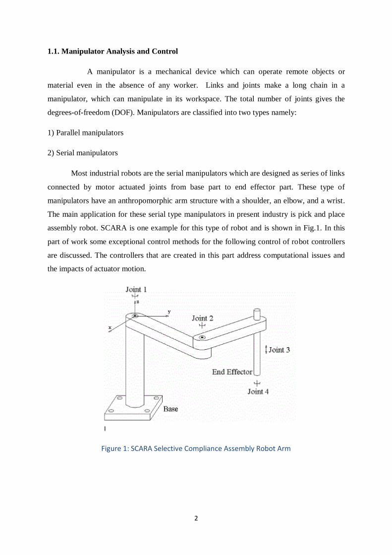
Most industrial robots are the serial manipulators which are designed as series of links

connected by motor actuated joints from base part to end effector part. These type of

manipulators have an anthropomorphic arm structure with a shoulder, an elbow, and a wrist.

The main application for these serial type manipulators in present industry is pick and place

assembly robot. SCARA is one example for this type of robot and is shown in Fig.1. In this

part of work some exceptional control methods for the following control of robot controllers

are discussed. The controllers that are created in this part address computational issues and

the impacts of actuator motion.

Figure 1: SCARA Selective Compliance Assembly Robot Arm

3

1.2. Literature Review

Literature survey was conducted to obtain some insights into various factors relating

to modelling of planar manipulators for various industrial applications. In this work several

aspects regarding the kinematics, workspace, Jacobian analysis and dynamic identification of

a two-link planar manipulator are studied and presented. De Luca and Siciliano [1] presented

the kinematic and dynamic issues of planar link manipulator. William [2] described

automatic Control Systems, analysis and design of serial manipulators. Kwanho [3] explained

the adaptive control of tip point in a serial link robot. Nagrath and Gopal [4] explained

various issues like kinematics, dynamics, control theories for different serial manipulators.

Tokhi and Azad [5] discussed the kinematic and modelling of flexible manipulators. Finally

the proposed control method is applied for the flexible manipulator to illustrate the results.

Ata [6] presented the review on various optimal trajectory planning control techniques for

serial manipulators. Islam and Liu [7] proposed a sliding mode control technique to serial

manipulator and studied the. Kumara et al. [8] explained trajectory tracking control of

kinematically redundant robot manipulators using neural network. Moldoveanu et al. [9]

explained a trajectory control of a two-link robot manipulator using variable structure theory.

Wang and Deng et al. [10] explained the design of articulated inspection arm with an

embedded camera and interchangeable tools. Zhu et al. [11] presented the structure of a serial

link robot with 8 degrees of freedom with a 3-axes wrist carrying camera. Ionescu [12]

described an approach of measurement using a calibrated Cr252 neutron source deployed by

in-vessel remote handling boom and mascot manipulator for J0ET vacuum vessel.

Monochrome CCD cameras were used as image sensors. Karagulle and Malgaca [13]

proposed the effect of flexibility on the trajectory of a planar two-link manipulator is studied

using integrated computer-aided design procedures. Nageshrao et al. [14] explained the

passivity based control method. Detailed algorithm was proposed and implemented for 2-

DOF manipulator. Ayala and Coelho [15] illustrated an algorithm to test the PID tuning by

using a two degree of freedom robot manipulator.

1.3. Objectives of the present work

In present work, the main objectives to be carried out are kinematic analysis, inverse

kinematic analysis, Jacobian analysis, dynamics and solution of dynamic equations. In the

part of results and discussions following things are presented: workspace analysis,

4

manipulability index, static force analysis, inverse dynamic analysis, control results and

model fabrication and control. For workspace analysis, a C program based on forward

kinematic equations is used. An Arduino program is used to control two servo motors for

tracking the given points with in the workspace. A Computed Torque Control scheme is used

to obtain the trajectory and a task space set point control approach is also presented.

The thesis is organised as follows: Chapter 2 describes mathematical modelling,

where the details of two link manipulator including dynamics are presented. Also control

algorithm based on CTC is given.

Chapter 3 describes the results and discussion as program outputs and experimentally

analysis outcomes.

Chapter 4 gives the brief conclusion.

5

Chapter 2

Mathematical Modelling

2.1. Kinematic Analysis

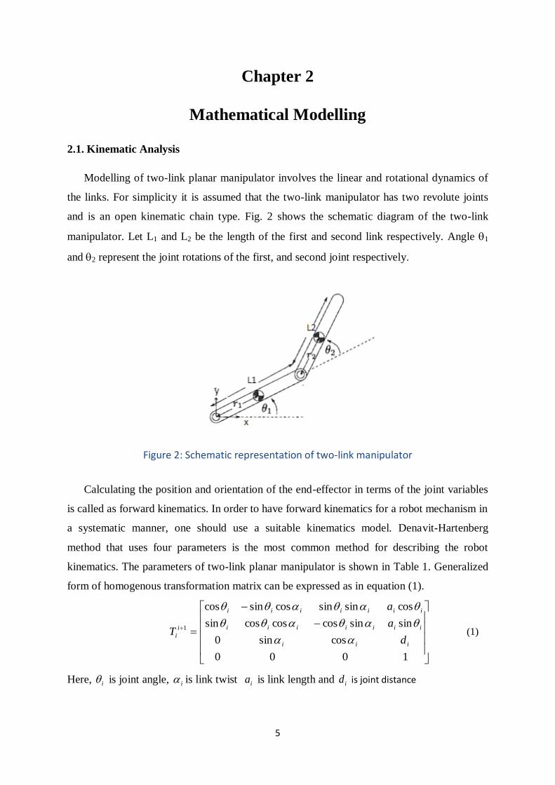
Modelling of two-link planar manipulator involves the linear and rotational dynamics of

the links. For simplicity it is assumed that the two-link manipulator has two revolute joints

and is an open kinematic chain type. Fig. 2 shows the schematic diagram of the two-link

manipulator. Let L1 and L2 be the length of the first and second link respectively. Angle 1

and 2 represent the joint rotations of the first, and second joint respectively.

Figure 2: Schematic representation of two-link manipulator

Calculating the position and orientation of the end-effector in terms of the joint variables

is called as forward kinematics. In order to have forward kinematics for a robot mechanism in

a systematic manner, one should use a suitable kinematics model. Denavit-Hartenberg

method that uses four parameters is the most common method for describing the robot

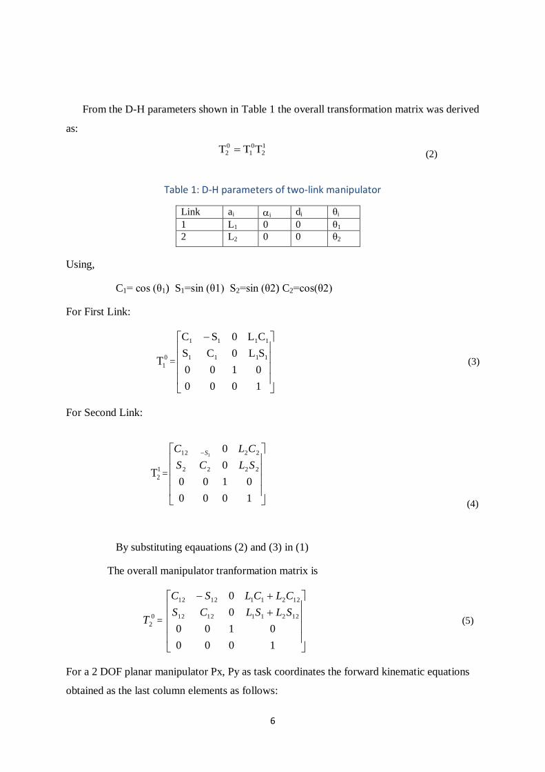
kinematics. The parameters of two-link planar manipulator is shown in Table 1. Generalized

form of homogenous transformation matrix can be expressed as in equation (1).

1000

cossin0

sinsincoscoscossin

cossinsincossincos

1

iii

iiiiiii

iiiiiii

i

id

a

a

T

(1)

Here, i is joint angle, i is link twist ia is link length and id is joint distance

6

From the D-H parameters shown in Table 1 the overall transformation matrix was derived

as:

12

01

02 TTT (2)

Table 1: D-H parameters of two-link manipulator

Link ai i di θi

1 L1 0 0 θ1

2 L2 0 0 θ2

Using,

C1= cos (θ1) S1=sin (θ1) S2=sin (θ2) C2=cos(θ2)

For First Link:

0

1T =

1000

0100

SL0CS

CL0SC

1111

1111

(3)

For Second Link:

1

2T =

1000

0100

0

0

2222

2212 1

SLCS

CLC S

(4)

By substituting eqauations (2) and (3) in (1)

The overall manipulator tranformation matrix is

0

2T =

1000

0100

0

0

122111212

122111212

SLSLCS

CLCLSC

(5)

For a 2 DOF planar manipulator Px, Py as task coordinates the forward kinematic equations

obtained as the last column elements as follows:

7

Px = L1cos θ1 + L2cos(θ1+ θ2) (6)

Py = L1sin θ1 + L2sin(θ1+ θ2) (7)

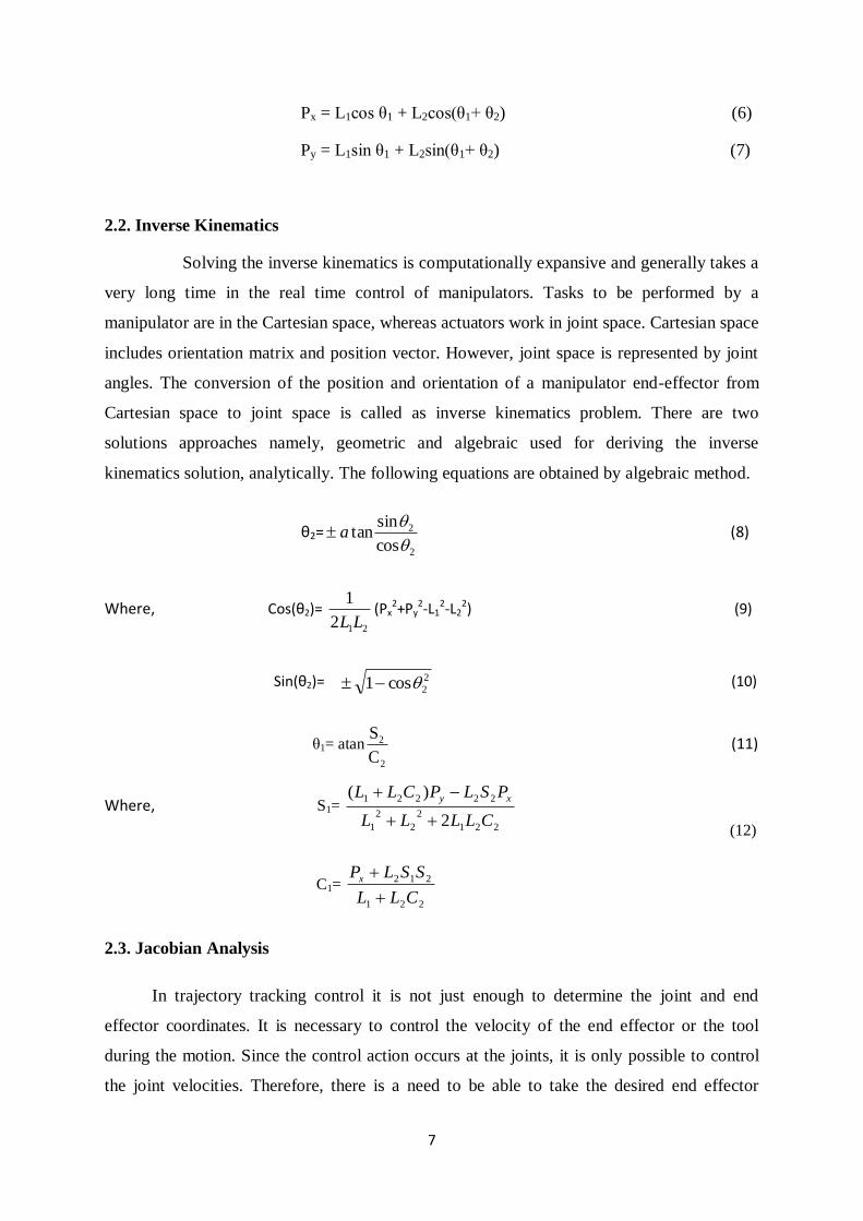
2.2. Inverse Kinematics

Solving the inverse kinematics is computationally expansive and generally takes a

very long time in the real time control of manipulators. Tasks to be performed by a

manipulator are in the Cartesian space, whereas actuators work in joint space. Cartesian space

includes orientation matrix and position vector. However, joint space is represented by joint

angles. The conversion of the position and orientation of a manipulator end-effector from

Cartesian space to joint space is called as inverse kinematics problem. There are two

solutions approaches namely, geometric and algebraic used for deriving the inverse

kinematics solution, analytically. The following equations are obtained by algebraic method.

θ2=2

2

cos

sintan

a (8)

Where, Cos(θ2)= 212

1

LL(Px

2+Py2-L1

2-L22) (9)

Sin(θ2)= 2

2cos1 (10)

θ1= atan2

2

C

S (11)

Where, S1=

221

2

2

2

1

22221

2

)(

CLLLL

PSLPCLL xy

(12)

C1= 221

212

CLL

SSLPx

2.3. Jacobian Analysis

In trajectory tracking control it is not just enough to determine the joint and end

effector coordinates. It is necessary to control the velocity of the end effector or the tool

during the motion. Since the control action occurs at the joints, it is only possible to control

the joint velocities. Therefore, there is a need to be able to take the desired end effector

8

velocities and calculate from them the joint velocities. Since we control the robot in joint

space and have a tendency to reason about movement in Cartesian space, we need to

completely comprehend the mapping from joint space to Cartesian space and the other way

around. Forward and inverse kinematics describes the static relationship between these

spaces.

The matrix which relates changes in joint parameter velocities to Cartesian velocities is

called the Jacobian Matrix. This is a time-varying, position dependent linear transform. It has

a number of columns equal to the number of degrees of freedom in joint space, and a number

of rows equal to the number of degrees of freedom in Cartesian space. The Jacobian for this

manipulator is:

The matrix which relates changes in joint parameter speeds to Cartesian speeds is known

as the Jacobian Matrix. It depends on time-varying, position dependent linear transform. It

has various sections equivalent to the quantity of degrees of freedom in joint space, and

number of rows equivalent to the degrees of freedom in Cartesian space. The Jacobian for

this planar manipulator is:

By differentiating the coordinates with respect to time

Y

X

= J

2

1

(13)

Here [J ]is Jacobian, [J] =

21

21

YY

XX

(14)

X = C1L1+L2C12 (15)

t

X

=

1

12211 )CLLC(

t

1

+

2

12211 )CLLC(

t

2

(16)

X = (-S1L1-L2S12) 1 -L2S12 2

(17)

Y = S1L1+L2S12 (18)

t

Y

=

1

12211 )SLLS(

t

1

+

2

12211 )SLLS(

t

2

(19)

Y = (C1L1+L2C12) 1 +L2C12 2

(20)

9

Y

X

=

21221211

21221211

CLCLLC

SLSLLS

2

1

(21)

X = J (22)

= J-1 X (23)

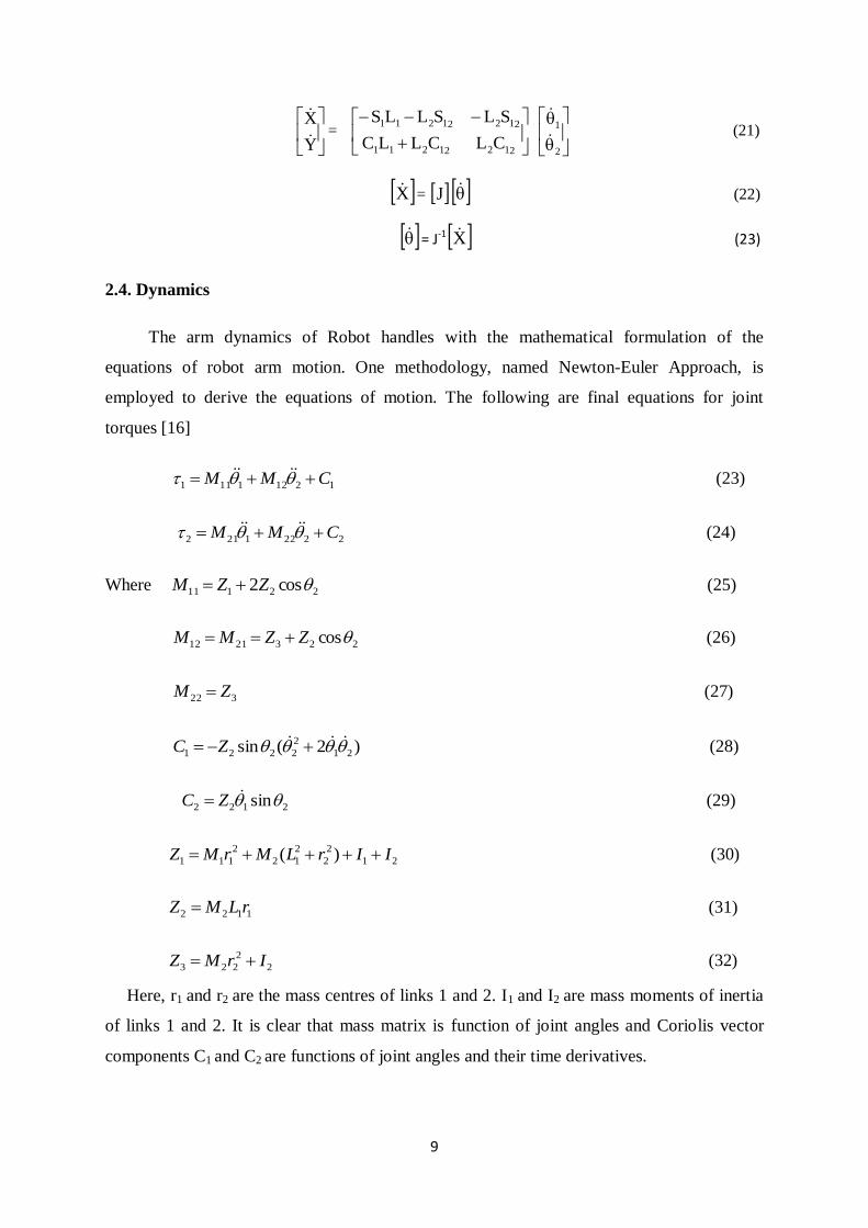
2.4. Dynamics

The arm dynamics of Robot handles with the mathematical formulation of the

equations of robot arm motion. One methodology, named Newton-Euler Approach, is

employed to derive the equations of motion. The following are final equations for joint

torques [16]

12121111 CMM (23)

22221212 CMM (24)

Where 22111 cos2 ZZM (25)

2232112 cosZZMM (26)

322 ZM (27)

)2(sin 21

2

2221 ZC (28)

2122 sinZC (29)

21

2

2

2

12

2

111 )( IIrLMrMZ (30)

1122 rLMZ (31)

2

2

223 IrMZ (32)

Here, r1 and r2 are the mass centres of links 1 and 2. I1 and I2 are mass moments of inertia

of links 1 and 2. It is clear that mass matrix is function of joint angles and Coriolis vector

components C1 and C2 are functions of joint angles and their time derivatives.

10

2.5. Solution of Dynamic Equations

Above dynamic equations are used for finding torques it is called inverse dynamics.

If torques are given and thetas are required, it is called forward dynamics. Forward dynamics

solution can be obtained by solving simultaneously two second order differential equations.

Generally numerical methods can be used for solving these equations. One of such technique

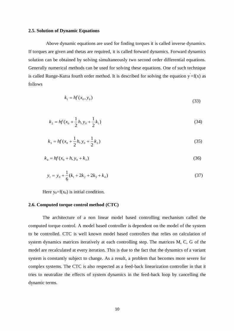
is called Runge-Kutta fourth order method. It is described for solving the equation y’=f(x) as

follows

),( 001 yxhfk (33)

)2

1,

2

1( 1002 kyhxhfk (34)

)2

1,

2

1( 2003 kyhxhfk (35)

),( 3004 kyhxhfk (36)

)22(6

1432101 kkkkyy (37)

Here y0=f(x0) is initial condition.

2.6. Computed torque control method (CTC)

The architecture of a non linear model based controlling mechanism called the

computed torque control. A model based controller is dependent on the model of the system

to be controlled. CTC is well known model based controllers that relies on calculation of

system dynamics matrices iteratively at each controlling step. The matrices M, C, G of the

model are recalculated at every iteration. This is due to the fact that the dynamics of a variant

system is constantly subject to change. As a result, a problem that becomes more severe for

complex systems. The CTC is also respected as a feed-back linearization controller in that it

tries to neutralize the effects of system dynamics in the feed-back loop by cancelling the

dynamic terms.

11

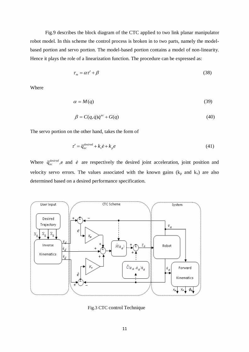
Fig.9 describes the block diagram of the CTC applied to two link planar manipulator

robot model. In this scheme the control process is broken in to two parts, namely the model-

based portion and servo portion. The model-based portion contains a model of non-linearity.

Hence it plays the role of a linearization function. The procedure can be expressed as:

m (38)

Where

)(qM (39)

)(),( qGqqqC ac (40)

The servo portion on the other hand, takes the form of

ekekq pv

desired

ac (41)

Where desired

acq ,e and e are respectively the desired joint acceleration, joint position and

velocity servo errors. The values associated with the known gains (kp and kv) are also

determined based on a desired performance specification.

Fig.3 CTC control Technique

12

Chapter 3

Results and Discussions

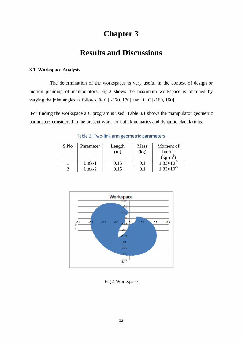
3.1. Workspace Analysis

The determination of the workspaces is very useful in the context of design or

motion planning of manipulators. Fig.3 shows the maximum workspace is obtained by

varying the joint angles as follows: θ1 ∈ [ -170, 170] and θ2 ∈ [-160, 160].

For finding the workspace a C program is used. Table.3.1 shows the manipulator geometric

parameters considered in the present work for both kinematics and dynamic claculations.

Table 2: Two-link arm geometric parameters

S.No Parameter Length

(m)

Mass

(kg)

Moment of

Inertia

(kg-m2)

1 Link-1 0.15 0.1 1.33×10-5

2 Link-2 0.15 0.1 1.33×10-5

Fig.4 Workspace

13

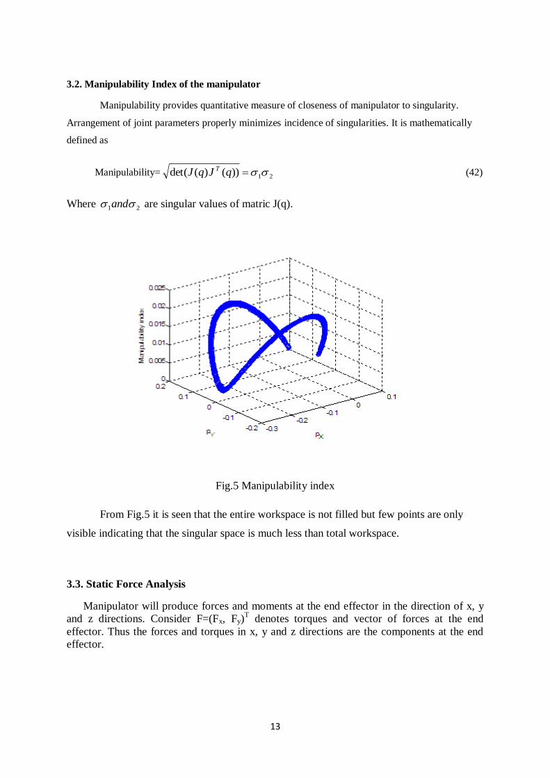
3.2. Manipulability Index of the manipulator

Manipulability provides quantitative measure of closeness of manipulator to singularity.

Arrangement of joint parameters properly minimizes incidence of singularities. It is mathematically

defined as

Manipulability= 21))()(det( qJqJ T (42)

Where 21 and are singular values of matric J(q).

Fig.5 Manipulability index

From Fig.5 it is seen that the entire workspace is not filled but few points are only

visible indicating that the singular space is much less than total workspace.

3.3. Static Force Analysis

Manipulator will produce forces and moments at the end effector in the direction of x, y

and z directions. Consider F=(Fx, Fy)T denotes torques and vector of forces at the end

effector. Thus the forces and torques in x, y and z directions are the components at the end

effector.

14

y

xT

F

FJ ][

2

1

(43)

By selecting joint space trajectories with a constant force Fx=10 N and Fy=10 N, we can plot

the joint torques. This analysis can be used for low speed applications.

Fig.6 Joint torque T1

15

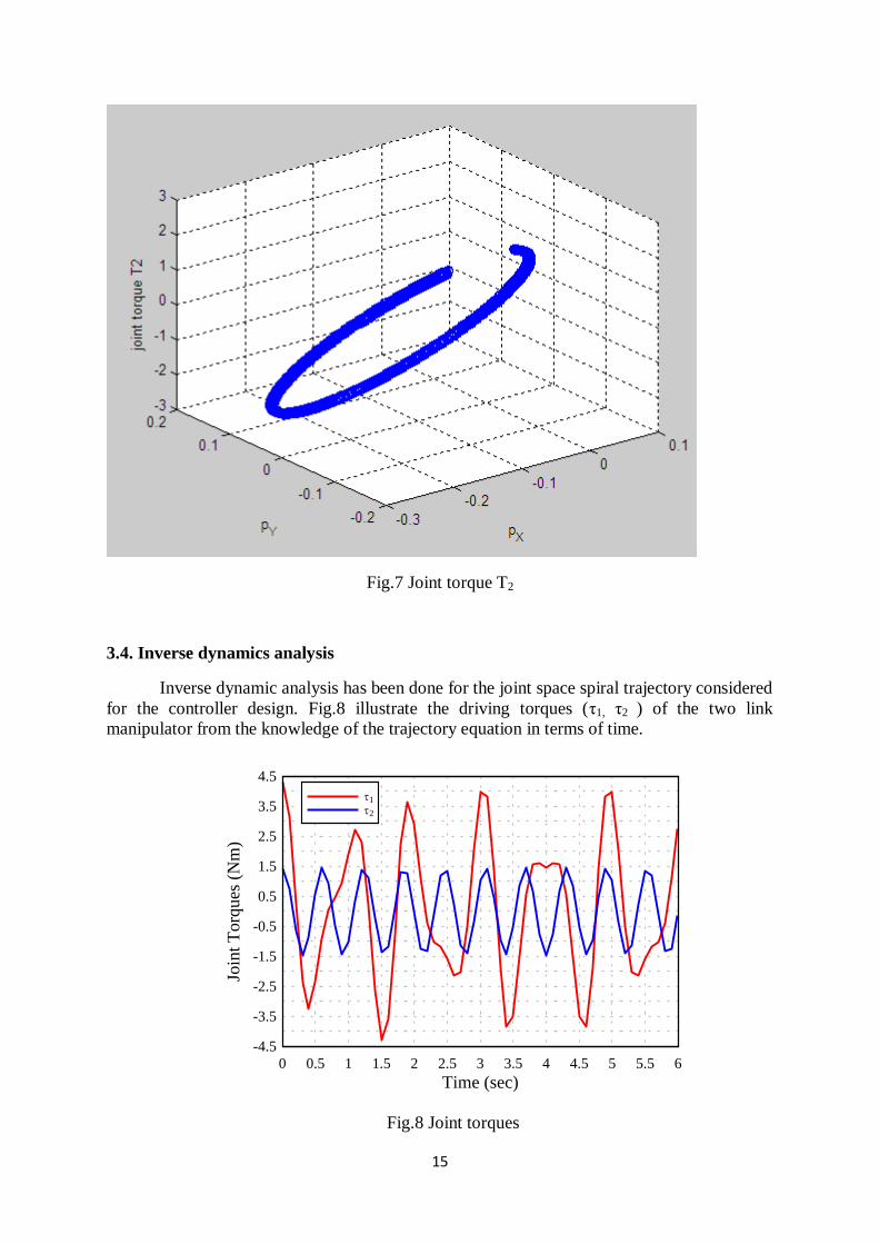
Fig.7 Joint torque T2

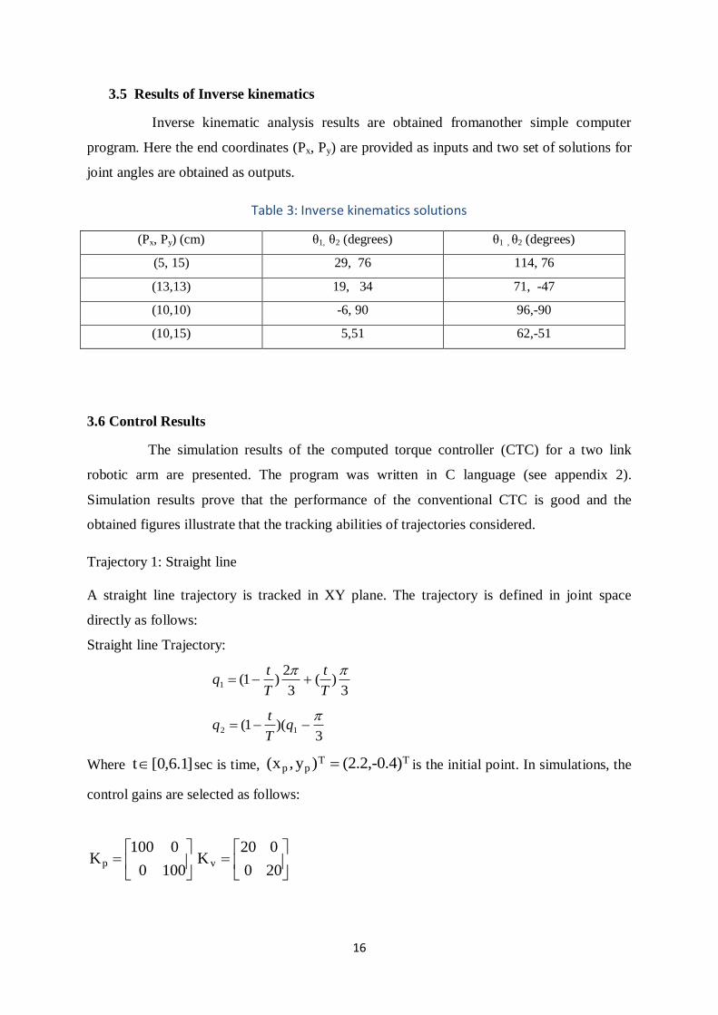
3.4. Inverse dynamics analysis

Inverse dynamic analysis has been done for the joint space spiral trajectory considered

for the controller design. Fig.8 illustrate the driving torques (τ1, τ2 ) of the two link

manipulator from the knowledge of the trajectory equation in terms of time.

Fig.8 Joint torques

Time (sec)

Join

t T

orq

ues

(N

m)

0 0.5 1 1.5 2 2.5 3 3.5 4 4.5 5 5.5 6

-4.5

-3.5

-2.5

-1.5

-0.5

0.5

1.5

2.5

3.5

4.5

1

2

16

3.5 Results of Inverse kinematics

Inverse kinematic analysis results are obtained fromanother simple computer

program. Here the end coordinates (Px, Py) are provided as inputs and two set of solutions for

joint angles are obtained as outputs.

Table 3: Inverse kinematics solutions

(Px, Py) (cm) θ1, θ2 (degrees) θ1 , θ2 (degrees)

(5, 15) 29, 76 114, 76

(13,13) 19, 34 71, -47

(10,10) -6, 90 96,-90

(10,15) 5,51 62,-51

3.6 Control Results

The simulation results of the computed torque controller (CTC) for a two link

robotic arm are presented. The program was written in C language (see appendix 2).

Simulation results prove that the performance of the conventional CTC is good and the

obtained figures illustrate that the tracking abilities of trajectories considered.

Trajectory 1: Straight line

A straight line trajectory is tracked in XY plane. The trajectory is defined in joint space

directly as follows:

Straight line Trajectory:

3

)(3

2)1(1

T

t

T

tq

3

)(1( 12

q

T

tq

Where ]1.6,0[t sec is time, TTpp (2.2,-0.4))y,x( is the initial point. In simulations, the

control gains are selected as follows:

1000

0100Kp

200

020Kv

17

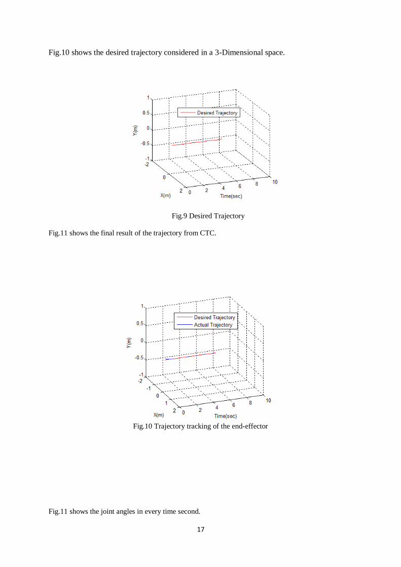
Fig.10 shows the desired trajectory considered in a 3-Dimensional space.

Fig.9 Desired Trajectory

Fig.11 shows the final result of the trajectory from CTC.

Fig.10 Trajectory tracking of the end-effector

Fig.11 shows the joint angles in every time second.

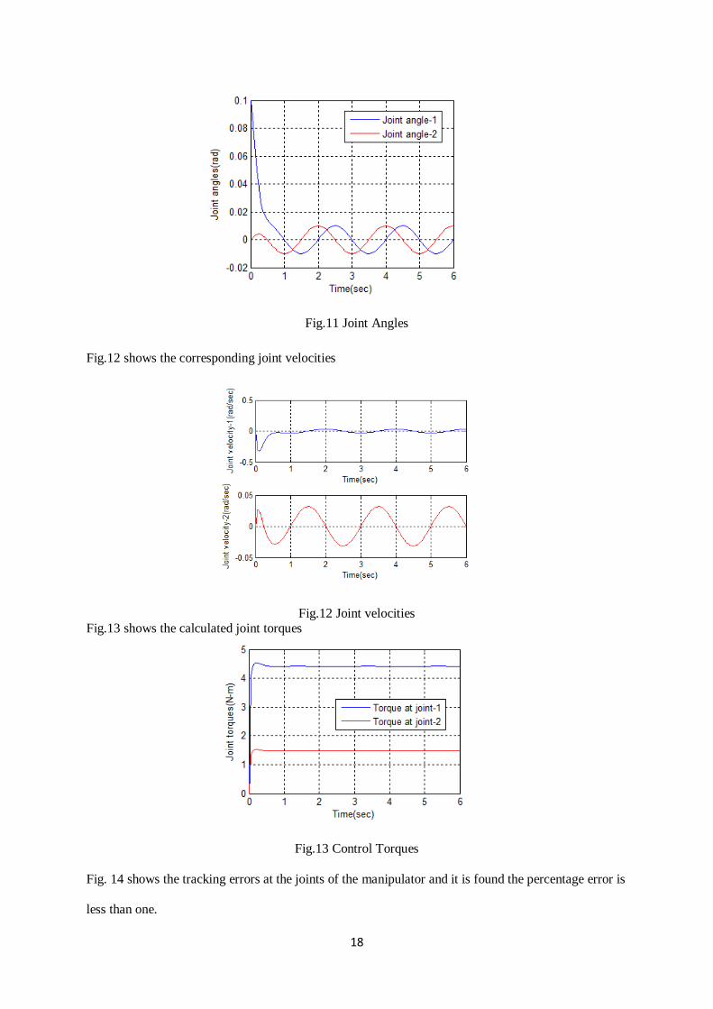
18

Fig.11 Joint Angles

Fig.12 shows the corresponding joint velocities

Fig.12 Joint velocities Fig.13 shows the calculated joint torques

Fig.13 Control Torques

Fig. 14 shows the tracking errors at the joints of the manipulator and it is found the percentage error is

less than one.

19

Fig.14 Tracking Errors

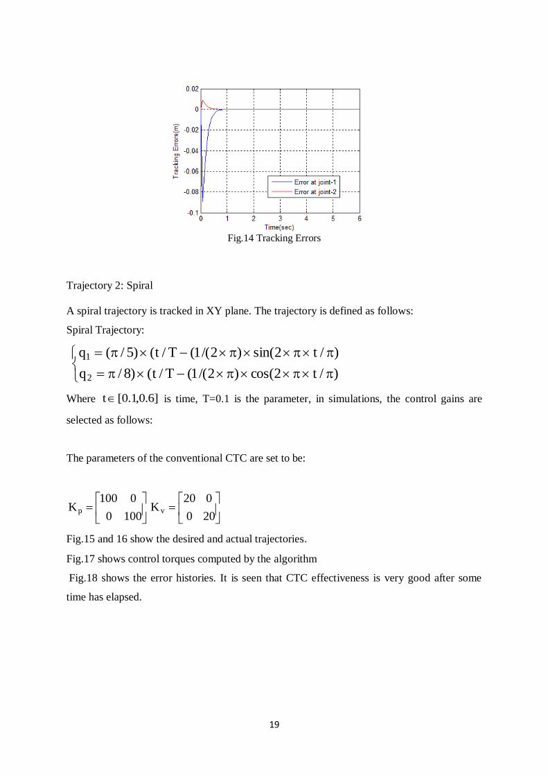
Trajectory 2: Spiral

A spiral trajectory is tracked in XY plane. The trajectory is defined as follows:

Spiral Trajectory:

)/t2cos()2/(1(T/t()8/q

)/t2sin()2/(1(T/t()5/(q

2

1

Where ]6.0,1.0[t is time, T=0.1 is the parameter, in simulations, the control gains are

selected as follows:

The parameters of the conventional CTC are set to be:

1000

0100Kp

200

020Kv

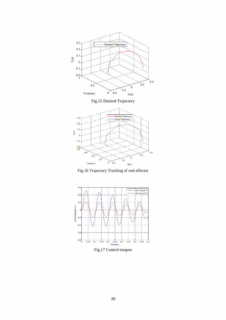
Fig.15 and 16 show the desired and actual trajectories.

Fig.17 shows control torques computed by the algorithm

Fig.18 shows the error histories. It is seen that CTC effectiveness is very good after some

time has elapsed.

20

Fig.15 Desired Trajectory

Fig.16 Trajectory Tracking of end effector

Fig.17 Control torques

21

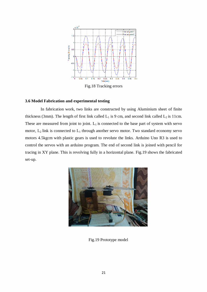
Fig.18 Tracking errors

3.6 Model Fabrication and experimental testing

In fabrication work, two links are constructed by using Aluminium sheet of finite

thickness (3mm). The length of first link called L1 is 9 cm, and second link called L2 is 11cm.

These are measured from joint to joint. L1 is connected to the base part of system with servo

motor, L2 link is connected to L1 through another servo motor. Two standard economy servo

motors 4.5kgcm with plastic gears is used to revolute the links. Arduino Uno R3 is used to

control the servos with an arduino program. The end of second link is joined with pencil for

tracing in XY plane. This is revolving fully in a horizontal plane. Fig.19 shows the fabricated

set-up.

Fig.19 Prototype model

22

Fig. 20 shows the control system based on laptop with an arduino board based on inverse

kinematics

Fig.20 Control experiment for tracking the points

The points are traced by giving the joint angles θ1 and θ2 to the arduino

microcontroller, which are obtained by the inverse kinematic equations and are shown in

Table.2. The corresponding code written in arduino compiler is shown below.

=====================================

#include<servo.h> servo servo 1; // define left servo

servo servo 2; // define right servo

void setup(){

servo 1.attach(10); // set left servo to digital pin 10

servo2.attach(9); // set right servo to digital pin 9

}

void loop() { // loop through motion test

p0();

delay(2000);

p1(); // example : move forward delay(2000); // wait 2000 milliseconds

p2();

delay(2000);

}

// motion routine for forward, reverse, turns, step

void p0() {

23

servo1.write(0);

servo2.write(0);

}

void p1(){

servo.write(0); servo2.write(180);

}

void p2(){

servo1.write(180);

servo2.write(0);

}

================================

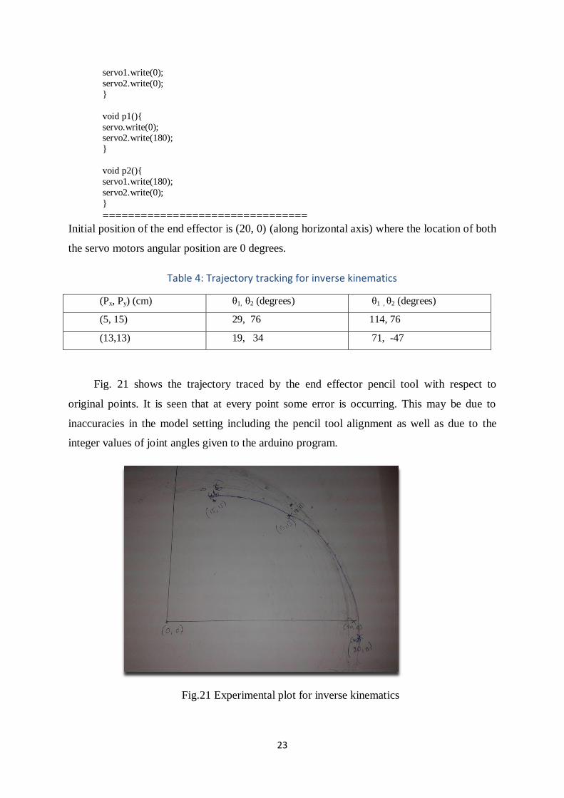
Initial position of the end effector is (20, 0) (along horizontal axis) where the location of both

the servo motors angular position are 0 degrees.

Table 4: Trajectory tracking for inverse kinematics

(Px, Py) (cm) θ1, θ2 (degrees) θ1 , θ2 (degrees)

(5, 15) 29, 76 114, 76

(13,13) 19, 34 71, -47

Fig. 21 shows the trajectory traced by the end effector pencil tool with respect to

original points. It is seen that at every point some error is occurring. This may be due to

inaccuracies in the model setting including the pencil tool alignment as well as due to the

integer values of joint angles given to the arduino program.

Fig.21 Experimental plot for inverse kinematics

24

Chapter 4

CONCLUSION

In this work several aspects regarding the kinematics, workspace, Jacobian analysis

and dynamic identification of a two-link planar manipulator were presented. The results

obtained in this study may be useful for the robot designing not only to understand the

kinematic behaviour of the robot for various configurations, but also to be able to implement

real time control of a manipulator. The programs are developed in C language for generation

of workspace points, manipulability index based on Jacobian and for inverse kinematics. The

results obtained are plotted separately from data files. Even though the two link manipulator

is relatively simple and straight forward, most of the approaches applied here are common to

all the manipulators. The static force analysis for obtaining joint torques is a important

problem for design of manipulator. Finally the trajectory tracking problem with two different

trajectories using CTC control method was illustrated numerically. The errors and

corresponding applied torques were shown as a function of time. This two link manipulator

analysis and control is an on going work in mechatronics and robotics research.

4.1. Future scope

The CTC control can be improved by tuning of position and velocity gain constants.

Also, when a disturbance such as a payload at the gripper acts on the system, the CTC

algorithm requires slight modification by adding additional control torque obtained from

disturbance rejection observer. This can be added to present work as a future scope. The

scaled model developed can be improved further to perform pick and place operations by

attaching a two finger gripper. This can be extended to a redundant four degree of freedom,

spatial SCARA manipulator with one translational joint. During the control, the manipulator

joint torques (hence angles) are to be computed automatically while tracking the trajectory is

going on. An improvised experimental work is required.

25

References

1) A. De Luca and B. Siciliano. Closed-Form Dynamic Model of Planar Multilink

Lightweight Robots. IEEE Trans. Syst., Man, Cybern. 1991; vol. 21, no. 4; pp. 826- 839.

2) A. W. William, Automatic Control Systems Basic Analysis and Design, Oxford

University Press, 1995; pp. 219-223.

3) Y. Kwanho. Adaptive Control, In-Tech publication, 2009; pp. 87-112.

4) I. J. Nagrath and M. Gopal, Control Systems Engineering, New Age Publisher, 2007.

5) M. O. Tokhi and A.K.M. Azad, Flexible Robot Manipulators Modeling, Simulation and

Control, IET, London, UK, 2008.

6) A. A. Ata. Optimal Trajectory Planning Of Manipulators: A review. J Engg. Sci. Tech.

2006; pp. 32–54.

7) S. Islam and X. P. Liu. Robust Sliding Mode Control for Robot Manipulators. IEEE

Trans. Ind. Elect. 2011; vol. 58; pp. 2444–2453.

8) N. Kumara, V. Panwarb and N. Sukavanamc. Neural Network-Based Nonlinear Tracking

Control of Kinematically Redundant Robot Manipulators. Math. Comp. Modelling.

2011; vol. 53; pp.1889–1901.

9) F. Moldoveanu, V. Comnac and D. Floroia. Trajectory Tracking Control of a Two-Link

Robot Manipulator using Variable Structure System Theory. Control Engg. App. Info.

2005; vol. 7; pp. 56–62.

10) A. Wang and M. Deng. Robust Nonlinear Control Design to a Manipulator Based on

Operator based Approach. ICIC Express Letters 2012; vol. 6; pp.617–623.

11) Y. Zhu, J. Qiu and J. Tani. Simultaneous Optimization of a Two-Link Flexible Robot

Arm. J. Robo. Syst. 2011; vol. 18; pp. 29–38.

12) F. Ionescu. Modeling and Simulation in Mechatronics. IFAS Int. Conf, MCPL 2007;

pp.26-29.

13) H. Karagulle and L. Malgaca, Analysis For End Point Vibrations Of Two Link

Manipulator By Integrated CAD/CAE Procedures. Finite Elem. Ana. Design. 2004; vol.

40; pp. 2049-2061.

14) S. P. Nageshrao, G. lopes, D. Jeltsema and R. Babuska. Passivity Based Reinforcement

Learning Control of a 2-DOF Manipulator Arm. Mechatronics. 2014; vol. 24; pp.1001-

1007.

15) H. V. H. Ayala, L. D. S. Coelho. Tuning of PID Controller Applied to a Robotic

Manipulator. Exp. Syst. App. 2012; vol. 39; pp. 8968-8974.

16) A. Wang and M. Deng, Robust non linear multi variable tracking control design to a

manipulator with unknown uncertainities using operator based robust right coprime

factorization, Transactions of institute of measurement and control, DOI

10.1177/0142331212470838, 2013.

26

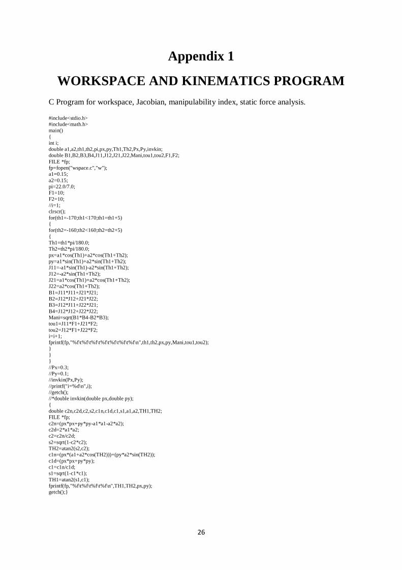
Appendix 1

WORKSPACE AND KINEMATICS PROGRAM

C Program for workspace, Jacobian, manipulability index, static force analysis.

#include<stdio.h>

#include<math.h>

main()

{

int i;

double a1,a2,th1,th2,pi,px,py,Th1,Th2,Px,Py,invkin;

double B1,B2,B3,B4,J11,J12,J21,J22,Mani,tou1,tou2,F1,F2;

FILE *fp;

fp=fopen("wspace.c","w");

a1=0.15;

a2=0.15;

pi=22.0/7.0;

F1=10;

F2=10;

//i=1;

clrscr();

for(th1=-170;th1<170;th1=th1+5)

{

for(th2=-160;th2<160;th2=th2+5)

{

Th1=th1*pi/180.0;

Th2=th2*pi/180.0;

px=a1*cos(Th1)+a2*cos(Th1+Th2);

py=a1*sin(Th1)+a2*sin(Th1+Th2);

J11=-a1*sin(Th1)-a2*sin(Th1+Th2);

J12=-a2*sin(Th1+Th2);

J21=a1*cos(Th1)+a2*cos(Th1+Th2);

J22=a2*cos(Th1+Th2);

B1=J11*J11+J21*J21;

B2=J12*J12+J21*J22;

B3=J12*J11+J22*J21;

B4=J12*J12+J22*J22;

Mani=sqrt(B1*B4-B2*B3);

tou1=J11*F1+J21*F2;

tou2=J12*F1+J22*F2;

i=i+1;

fprintf(fp,"%f\t%f\t%f\t%f\t%f\t%f\t%f\n",th1,th2,px,py,Mani,tou1,tou2);

}

}

}

//Px=0.3;

//Py=0.1;

//invkin(Px,Py);

//printf("i=%d\n",i);

//getch();

//*double invkin(double px,double py);

{

double c2n,c2d,c2,s2,c1n,c1d,c1,s1,a1,a2,TH1,TH2;

FILE *fp;

c2n=(px*px+py*py-a1*a1-a2*a2);

c2d=2*a1*a2;

c2=c2n/c2d;

s2=sqrt(1-c2*c2);

TH2=atan2(s2,c2);

c1n=(px*(a1+a2*cos(TH2)))+(py*a2*sin(TH2));

c1d=(px*px+py*py);

c1=c1n/c1d;

s1=sqrt(1-c1*c1);

TH1=atan2(s1,c1);

fprintf(fp,"%f\t%f\t%f\t%f\n",TH1,TH2,px,py);

getch();}

27

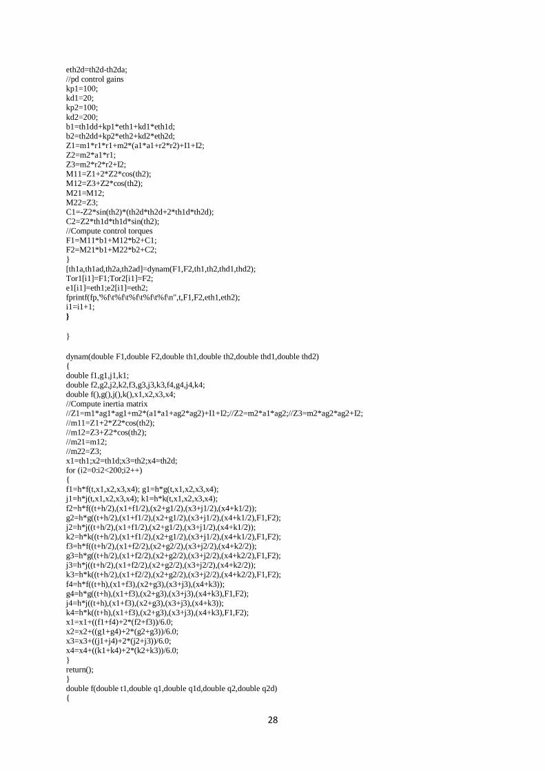
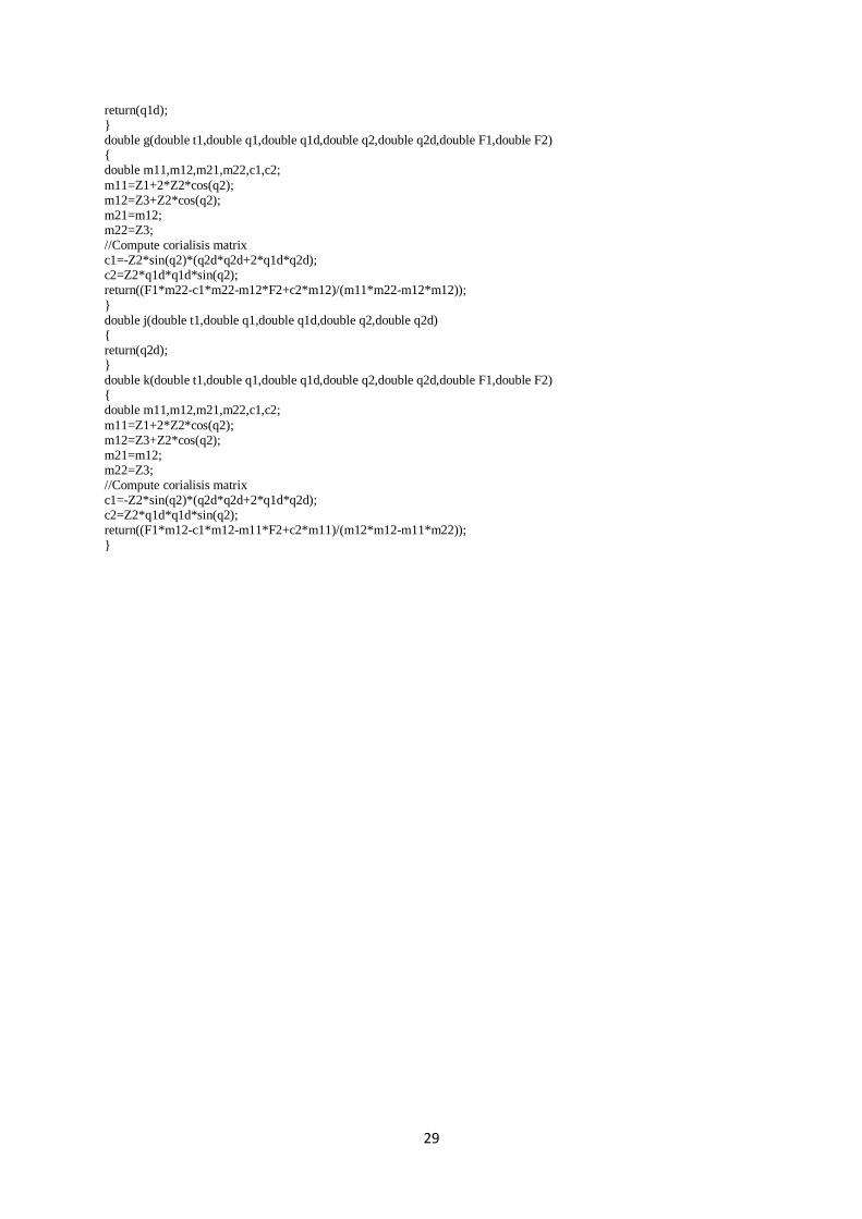
Appendix 2

CTC PROGRAM IN ‘C” LANGUAGE

C Programming code for CTC control.

#include<stdio.h>

#include<math.h> #define m1 0.1 #define m2 0.1 #define a1 0.15 #define a2 0.15 #define Z1 #define Z2 #define Z3

main() { int i; double kp1,kd1,kp2,kd2,px,py,px0,py0,pxd,pyd,pxdd,pydd,t,r,pi,X,Xa,Xd,c2n,c2d,c2,s2; double thd,th1,th2,c1n,cld,c1,s1,J[2][2],JT[2][2],JI[2][2],e[2][1],ed[2][1]; double a1,a2,F1,F2; FILE *fp; fp=fopen("dynamic.c","w");

px0=0.3; py0=0.3; r=0.01; pi=22.0/7.0; i=0; //desired trajectory for(t=0;t<2*pi;t=t+0.01) {

px=px0+r*cos(t); py=py0+r*sin(t); pxd=-r*sin(t); pyd=r*cos(t); pxdd=-r*cos(t); pydd=-r*sin(t); //Inverse kinematics c2=(px*px+py*py-a1*a1-a2*a2)/(2*a1*a2); s2=sqrt(1-c2*c2);

th2=atan2(s2,c2); s1=((a1+a2*c2)*py-px*a2*s2)/(a1*a1+a2*a2+2*a1*a2*c2); c1=(px+s1*a2*s2)/(a1+a2*c2); th1=atan2(s1,c1); // JACOBIAN J[0][0]=-s1*a1-a2*sin(th1+th2); J[0][1]=-a2*sin(th1+th2); J[1][0]=c1*a1+a2*cos(th1+th2);

J[1][1]=a2*cos(th1+th2); detJ=J[0][0]*J[1][1]-J[0][1]*J[1][0]; JI[0][0]=J[0][0]/detJ;JI[0][1]=-J[1][0]/detJ; JI[1][0]=-J[0][1]/detJ;JI[1][1]=J[1][1]/detJ; th1d=JI[0][0]*pxd+JI[0][1]*pyd; th2d=JI[1][0]*pxd+JI[1][1]*pyd; if(i==0) {

F1=rand(); F2=rand(); } else { //compute errors eth1=th1-th1a; eth2=th2-th2a;

eth1d=th1d-th1da;

28

eth2d=th2d-th2da; //pd control gains kp1=100; kd1=20; kp2=100;

kd2=200; b1=th1dd+kp1*eth1+kd1*eth1d; b2=th2dd+kp2*eth2+kd2*eth2d; Z1=m1*r1*r1+m2*(a1*a1+r2*r2)+I1+I2; Z2=m2*a1*r1; Z3=m2*r2*r2+I2; M11=Z1+2*Z2*cos(th2); M12=Z3+Z2*cos(th2);

M21=M12; M22=Z3; C1=-Z2*sin(th2)*(th2d*th2d+2*th1d*th2d); C2=Z2*th1d*th1d*sin(th2); //Compute control torques F1=M11*b1+M12*b2+C1; F2=M21*b1+M22*b2+C2; }

[th1a,th1ad,th2a,th2ad]=dynam(F1,F2,th1,th2,thd1,thd2); Tor1[i1]=F1;Tor2[i1]=F2; e1[i1]=eth1;e2[i1]=eth2; fprintf(fp,'%f\t%f\t%f\t%f\t%f\n",t,F1,F2,eth1,eth2); i1=i1+1;

}

}

dynam(double F1,double F2,double th1,double th2,double thd1,double thd2) { double f1,g1,j1,k1; double f2,g2,j2,k2,f3,g3,j3,k3,f4,g4,j4,k4; double f(),g(),j(),k(),x1,x2,x3,x4; //Compute inertia matrix //Z1=m1*ag1*ag1+m2*(a1*a1+ag2*ag2)+I1+I2;//Z2=m2*a1*ag2;//Z3=m2*ag2*ag2+I2;

//m11=Z1+2*Z2*cos(th2); //m12=Z3+Z2*cos(th2); //m21=m12; //m22=Z3; x1=th1;x2=th1d;x3=th2;x4=th2d; for (i2=0:i2<200;i2++) { f1=h*f(t,x1,x2,x3,x4); g1=h*g(t,x1,x2,x3,x4); j1=h*j(t,x1,x2,x3,x4); k1=h*k(t,x1,x2,x3,x4);

f2=h*f((t+h/2),(x1+f1/2),(x2+g1/2),(x3+j1/2),(x4+k1/2)); g2=h*g((t+h/2),(x1+f1/2),(x2+g1/2),(x3+j1/2),(x4+k1/2),F1,F2); j2=h*j((t+h/2),(x1+f1/2),(x2+g1/2),(x3+j1/2),(x4+k1/2)); k2=h*k((t+h/2),(x1+f1/2),(x2+g1/2),(x3+j1/2),(x4+k1/2),F1,F2); f3=h*f((t+h/2),(x1+f2/2),(x2+g2/2),(x3+j2/2),(x4+k2/2)); g3=h*g((t+h/2),(x1+f2/2),(x2+g2/2),(x3+j2/2),(x4+k2/2),F1,F2); j3=h*j((t+h/2),(x1+f2/2),(x2+g2/2),(x3+j2/2),(x4+k2/2)); k3=h*k((t+h/2),(x1+f2/2),(x2+g2/2),(x3+j2/2),(x4+k2/2),F1,F2);

f4=h*f((t+h),(x1+f3),(x2+g3),(x3+j3),(x4+k3)); g4=h*g((t+h),(x1+f3),(x2+g3),(x3+j3),(x4+k3),F1,F2); j4=h*j((t+h),(x1+f3),(x2+g3),(x3+j3),(x4+k3)); k4=h*k((t+h),(x1+f3),(x2+g3),(x3+j3),(x4+k3),F1,F2); x1=x1+((f1+f4)+2*(f2+f3))/6.0; x2=x2+((g1+g4)+2*(g2+g3))/6.0; x3=x3+((j1+j4)+2*(j2+j3))/6.0; x4=x4+((k1+k4)+2*(k2+k3))/6.0;

} return(); } double f(double t1,double q1,double q1d,double q2,double q2d) {

29

return(q1d); } double g(double t1,double q1,double q1d,double q2,double q2d,double F1,double F2) { double m11,m12,m21,m22,c1,c2;

m11=Z1+2*Z2*cos(q2); m12=Z3+Z2*cos(q2); m21=m12; m22=Z3; //Compute corialisis matrix c1=-Z2*sin(q2)*(q2d*q2d+2*q1d*q2d); c2=Z2*q1d*q1d*sin(q2); return((F1*m22-c1*m22-m12*F2+c2*m12)/(m11*m22-m12*m12));

} double j(double t1,double q1,double q1d,double q2,double q2d) { return(q2d); } double k(double t1,double q1,double q1d,double q2,double q2d,double F1,double F2) { double m11,m12,m21,m22,c1,c2;

m11=Z1+2*Z2*cos(q2); m12=Z3+Z2*cos(q2); m21=m12; m22=Z3; //Compute corialisis matrix c1=-Z2*sin(q2)*(q2d*q2d+2*q1d*q2d); c2=Z2*q1d*q1d*sin(q2); return((F1*m12-c1*m12-m11*F2+c2*m11)/(m12*m12-m11*m22));

}