Summary Report

WP5 - Developing existing grass growth model to make use of remotely sensed data

Authors: Isabel Whiteley, Louise Willingham, Ben Hockridge, Steven Anthony, Pete Berry; RSK ADAS Ltd

Introduction Aim Make use of information and understanding developed from previous WPs to develop existing grass growth model so they can make use of remotely sensed information. Carry out preliminary tests using independent data collected as part of the project to assess the potential benefit of using this remotely sensed information.

Approach Select a model to develop based on conclusions from WP2 and available data.

Build a working version of the model, including functionality enabling use of remotely-sensed (satellite) information. Set up model to test use of remotely-sensed data in two ways: 1. Update model biomass based on remotely-sensed estimates of biomass. 2. Calibrate model parameters so that model predictions match remotely sensed estimates of biomass as closely as possible.

Calibrate model for UK based on GM20 trial data.

Trial calibration of model with remote sensing data.

Compare model predictions (before and after calibration from remote sensing data) against ground measurements to gauge success of using remote sensing data.

Findings from Work Packages 2 and 3 Many of the grass growth models considered in the review in work package 2 require a large number of site-specific inputs (for example clover content and soil N content). For the ongoing development in work package 5, we required a model that could be run with a minimal number of site-specific inputs to enhance the accessibility of the model as a tool to farmers. Given the aim to use remotely-sensed (satellite) data to update model biomass and/or calibrate model parameters, models having a simple biomass pool structure and a few key parameters describing site productivity were the best-suited to the task. A model where the code was freely available or for which the model equations were fully described in published papers was also required to enable further model development. Based on these criteria, the PGSUS model described in Romera et al. (2009, 2010), which is an updated version of the model described by McCall (1984, 2003), was selected for further development in work package 5.

In work package 3, it was found that optical (combination of visible and infra-red spectrum) data had the best predictive ability for estimating ryegrass standing biomass, and radar data was less promising for this purpose. However, the availability of optical satellite data is constrained by cloud cover,

restricting the number of satellite estimates available for a single farm in any one year. Combining a grass growth model with satellite data will potentially provide an effective method of remotely estimating grass growth since the satellite data can be used to periodically ‘re-set’ the model to keep it on track, and/or to calibrate the model to improve its site-specific performance. The yard-stick against which to calibrate and test the model of grass growth is farmer-measured data (e.g. rising plate meter estimates of biomass), since this is the measurement that farmers use to make commercial decisions.

Spreadsheet implementation of PGSUS model and model developments An implementation of the model described in Romera et al. (2010) was built in Microsoft Excel. Following initial exploration of the outputs provided by the model, it was necessary to make some changes to the model to improve the simulation of grass growth in UK conditions. The model equations are described in full in an index within the model spreadsheet, but the changes made are described briefly below. The PGSUS model described in Romera et al. (2010) simulates green herbage mass only, but when the grass is not very regularly grazed then simulation of senesced biomass pools becomes increasingly important. The McCall and Bishop-Hurley model (2003) on which PGSUS is based does include senesced biomass pools. Soluble and insoluble senesced biomass are tracked separately, with differing processes affecting the rate of loss of each senesced pool. This functionality was therefore reintroduced to the spreadsheet model. Soluble biomass is lost through leaching and microbial action (the rates of which are driven in the model by daily temperature and rainfall), and insoluble biomass is lost through microbial action (at a lower rate than soluble biomass) and earthworm action. The PGSUS model includes a factor, gT, to describe the effects of temperature on growth. The value of gT ranges from 0 to 1, where 1 is no inhibition on growth as a result of temperature, and 0 is complete inhibition on growth as a result of temperature. The temperature factors described in Romera et al (2009) and McCall and Bishop-Hurley (2003) were both considered, but it was decided to substitute the relationship between temperature and grass growth used by Brereton et al. (1996), converted into a multiplier ranging from 0 to 1, as this shows a more gradual increase in growth rate at low temperatures. A comparison of the growth factors is given in Figure 1.

Figure 1 Comparison of parameters describing the effect of temperature on relative grass growth (gT) in Brereton (1996), McCall (2003) and Romera (2009) papers.

The PGSUS model is calibrated to each site by changing two parameters that affect the radiation-use efficiency and two parameters that represent the available soil water holding capacity. The soil water properties in the spreadsheet implementation of the model model are instead determined by the generic soil type and do not require specific calibration. The soil types included in the spreadsheet model are clay, silty clay, sandy clay, clay loam, silt loam, sandy loam, loamy sand, sand, peaty loam and loamy peat. Waterlogging as well as moisture stress can significantly limit grass growth (Laidlaw, 2009). A water table model was introduced to represent the impact of waterlogging, restricting growth on days when the water table was high; this is expected to have the most impact on heavier clay soils.

The water table model considers two flows (vertical and lateral) in order to determine the position of the water table, relative to the soil surface. The Hooghoudt formula, taken from Smedema and Rycroft (1983), is used to calculate the vertical flow at time t, qt:

𝑞𝑡 =8𝐾𝑑ℎ𝑡−1

𝐿2+

4𝐾ℎ𝑡−12

𝐿2

where K is the Vertical Hydraulic Conductivity (m day-1), d is the depth of soil (m), ht-1 is the previous height of the water table (m) at time t-1 and L is the average distance between drains (m). K and d are averages for the soil type. L is the county average taken from a DEFRA database of agricultural drainage (ADAS report to DEFRA, 2002). Darcy’s Law is used to calculate lateral flow to be drained away. This accounts for a field slope at an angle greater than 0°:

𝑞𝑙𝑎𝑡 =𝑑ℎ𝐾𝑙𝑎𝑡

𝐹

where hi is the difference in height (m) between the top of the field and the bottom of the field, Klat

is the lateral hydraulic conductivity (m/day) and F is the slope length (m). hi is calculated as:

ℎ𝑖 = tan(𝑆 (2𝜋

360))𝐹

where S is the slope of the field (degrees). By default, S is assumed to be 0.1 degrees and F is assumed to be 600m. Once the vertical and lateral flows are calculated, they are subtracted from the previous day’s water table height. Recharge water in excess of the available soil water capacity, Rt, is calculated as the rainfall less the previous day’s soil moisture deficit, and is added to the previous day’s water table height through the de Zeeuw-Hellinga formula (Smedema and Rycroft, 1983):

ℎ𝑡 = ℎ𝑡−1 +𝑅𝑡

0.8𝜇

where ht is the water table height (m) at time t, ht-1 is the water table height (m) at time t-1, and μ is the average available pore space (%) for the soil type. This is calculated at a timestep, t, of 0.01 days, assuming that Rt arrives at a constant rate throughout the day. If the calculated height is <0m, it is set equal to 0m. This new water table height is taken from the full depth of the soil profile, to indicate the depth of soil which contains air. This is used to give the waterlogging factor, gwl. Following Bennett et al. (2009), gwl is a linear scale between 1-0, where 1 = normal growth and 0 = no growth. When the water table is within 20cm of the surface, the roots in this zone are under anoxic conditions and the plant becomes stressed. It is assumed that 90% of the grass roots are in the top 10cm of soil, and capillary rise may mobilise water from around another 20cm away (Bennett et al., 2009). As the water table rises towards the surface, grass growth becomes restricted.

The model parameters a and b describe the growth response to radiation through the parameter α:

𝛼 = 𝑏

1 − exp (−𝑎 × 𝐼)

where, from Romera et al. (2010), ‘α is the radiation-use efficiency for radiation in MJ when there are no other climatic or light interception constraints, I is the incident solar radiation (MJ/m2/day), a is the constant determining the shape of the function, and b is the asymptotic value of α when the growth response to I reaches saturation’. A large value of a indicates that the response to light is not strongly seasonal, whereas a small value of a indicates that the radiation-use efficiency is higher at low light levels. The PGSUS model uses a simple equation that adds additional new growth at a fixed rate for each kg of nitrogen applied and does not take account of other factors affecting this additional growth or the strength of the growth response to nitrogen. It was decided not to use this equation in the spreadsheet implementation, but instead to use the parameter b to represent the growth potential of a field in response to nitrogen availability and other factors. The model requires the following inputs to run:

Daily weather data: solar radiation (MJ/m2/day), daily minimum and maximum temperature (oC), daily mean temperature (oC) (optional, if not available this is estimated as the average of the minimum and maximum daily temperature), rainfall (mm/day) and average windspeed (m/s).

Site location.

Soil texture type (clay, silty clay, sandy clay, clay loam, silt loam, sandy loam, loamy sand, sand, peaty loam or loamy peat).

Additionally, site elevation, field slope and slope length may be given as inputs – if not supplied then model defaults will be used (elevation 10m, field slope 0.1o, slope length 600m).

The spreadsheet model was set up so that the total biomass could be reset using a satellite estimate or farmer measurement (e.g. using a sward stick) of total above ground biomass, or through the farmer entering a grazing event (the biomass following grazing may be entered, otherwise 1500 kg DM/ha is the assumed default value). The change in the total biomass is distributed amongst the green, soluble senesced and insoluble senesced biomass pools in proportion to the fraction of each as a proportion of the total biomass on the previous day.

Calibration to ADAS/GRI Grassland Manuring Trials (GM20 dataset) The model parameters a and b were calibrated for UK conditions using a dataset from grass growth trials carried out between 1970 and 1974 (Morrison et al. 1980). The dataset comprises the mean perennial ryegrass yield at six cut dates over four years, and total yield per year for each of four years, for six different fertilizer N rates (0, 150, 300, 450, 600 and 750 kg N/ha) at 21 sites across England and Wales. The spreadsheet model was set up for each site and nitrogen level and the values of a and b optimised together for each site using the Excel Solver with the ‘GRG Nonlinear’ setting (other Excel Solver options such as ‘Multistart’ and ‘Evolutionary’ algorithms were trialled, but it was found that the additional runtime was not matched by a substantial improvement in fit). One overall value of a was used for each site, whereas the value of b was allowed to vary by N rate, with the constraint that, for a given N rate, the value of b must be greater than or equal to the value of b for the N rate below it.

50% of the sites had fitted values of a between 0.176 and 0.265 (Figure 2). There were no obvious patterns in the fitted values of a by region, soil type, elevation, annual or seasonal rainfall,

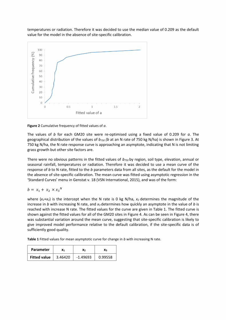
temperatures or radiation. Therefore it was decided to use the median value of 0.209 as the default value for the model in the absence of site-specific calibration.

Figure 2 Cumulative frequency of fitted values of a.

The values of b for each GM20 site were re-optimised using a fixed value of 0.209 for a. The geographical distribution of the values of b750 (b at an N rate of 750 kg N/ha) is shown in Figure 3. At 750 kg N/ha, the N rate response curve is approaching an asymptote, indicating that N is not limiting grass growth but other site factors are.

There were no obvious patterns in the fitted values of b750 by region, soil type, elevation, annual or seasonal rainfall, temperatures or radiation. Therefore it was decided to use a mean curve of the response of b to N rate, fitted to the b parameters data from all sites, as the default for the model in the absence of site-specific calibration. The mean curve was fitted using asymptotic regression in the ‘Standard Curves’ menu in Genstat v. 18 (VSN International, 2015), and was of the form:

𝑏 = 𝑥1 + 𝑥2 × 𝑥3𝑁

where (x1+x2) is the intercept when the N rate is 0 kg N/ha, x2 determines the magnitude of the increase in b with increasing N rate, and x3 determines how quickly an asymptote in the value of b is reached with increase N rate. The fitted values for the curve are given in Table 1. The fitted curve is shown against the fitted values for all of the GM20 sites in Figure 4. As can be seen in Figure 4, there was substantial variation around the mean curve, suggesting that site-specific calibration is likely to give improved model performance relative to the default calibration, if the site-specific data is of sufficiently good quality.

Table 1 Fitted values for mean asymptotic curve for change in b with increasing N rate.

Parameter x1 x2 x3

Fitted value 3.46420 -1.49693 0.99558

Figure 3 Geographical distribution of fitted values of b750.

Figure 4 Change in fitted value of b with increasing N rate at GM20 sites.

The relationship between the value of b and the predicted average annual grass yield (from six cuts per year down to a residual of 5cm, assumed to equate to 1500 kg DM/ha) for the four years of the experiment is shown in Figure 5, illustrating how the model can be calibrated to match the growth potential of an individual field or farm by changing the value of this parameter. Site-specific factors such as weather and soil type also affect the model predictions of yield.

Figure 5 Change in fitted value of b with increasing N rate at GM20 sites.

Calibration using satellite data The satellite calibration from Landsat 8 imagery, based on a calibration at a single farm in Exeter using WDRVI as shown in the report on WP3 in Figure 8(e), was used to test the use of satellite estimates of above-ground biomass for calibration and resetting of the model at Hall Farm in Norfolk. This meant that Hall Farm in Norfolk was a test dataset, and the satellite calibration used was completely independent of the test dataset. The satellite calibration developed in WP4 used data from multiple sites across a number of geographical locations, including Hall Farm, so was not used for this test as it would not have been independent but could be used in future work for this purpose.

The model was set up for 5 fields at Hall Farm in Norfolk. The soil type ‘clay loam’ was used. Data was available for both 2016 and 2017. All recorded grazing events were entered into the model so that the biomass was updated after each grazing event. As the residual biomass had not been recorded immediately following each grazing/cutting event, a residual biomass of 1500 kg DM/ha was assumed. Weather data was sourced from MetMake, run from within IRRIGUIDE 4.3 (© ADAS 2006, Silgram 2007, Bailey and Spackman, 1996).

Satellite estimates of biomass were available for each field on 5 dates in 2016 (16/02/16, 20/04/16, 07/06/16, 18/07/16 and 28/08/16) and 1 date in 2017 (15/03/17) – a total of 30 data points. Two data points were omitted because they coincided with grazing dates on the relevant paddocks. The remaining 28 data points were all used for the model re-setting and calibration.

For the default model, a was set at 0.209 and an N rate of 300 kg N/ha was assumed based on 2017 fertiliser data and the size of the herd (160 cows), giving a default b parameter value of 3.068 g DM/MJ.

Using the default model calibration, the use of satellite data to initialise the value of the model biomass pool was compared with a default estimate of 1500 kg DM/ha and with farmer-measured data. To test the performance of the model without input from either satellite estimates of rising plate meter measurements, using only soil type, farm location and field grazing dates, the default model was initialised with an estimated biomass of 1500 kg DM/ha on 01/01/16. The R2 of the model predictions for a total of 183 rising plate meter measurements taken in the fields between 22/02/16 and 31/10/16 was calculated as 53.3%, and for 90 rising plate meter measurements taken between 30/01/17 and 29/05/17 was calculated as 68.9%. Next, the model biomass was re-set using satellite estimates of biomass from 16/02/16 only. The R2 for the 2016 measurements increased to 66.5% following the single re-set, and remained the same to 3 significant figures (s.f.) for the 2017 measurements (68.9%). Next, the initial biomass was set from rising plate measurements taken in each field on 01/02/16. This resulted in an increased R2 for the 2016 measurements of 67.7%, whilst the R2 for the 2017 measurements again remained at 68.9% to 3 s.f.. These results show that in this case, initialisation with satellite biomass estimates improved the model fit relative to a naïve estimate of initial biomass, and was almost as effective as initialisation with farmer-measured biomass values.

The model initialised with farmer-measured data from 01/02/16 was used for all further comparisons detailed below. Therefore weekly measurements taken on 08/02/16 and 15/02/16 could also be included in the dataset, so the R2 for the model predictions was calculated for: i.) 193 rising plate meter measurements taken between 08/02/16 and 31/10/16 and 90 rising plate meter measurements taken between 30/01/17 and 29/05/17. In addition, the R2 was calculated for a restricted dataset ii.), with measurements of biomass above 3500 kg DM/ha excluded from the dataset, leaving 186 rising plate meter measurements taken between 08/02/16 and 31/10/16 and 86 rising plate meter measurements taken between 30/01/17 and 29/05/17. The restricted dataset was included because the WDRVI calibration used from WP3 was based on measured grass biomass values up to approximately 3100 kg DM/ha. None of the vegetation indices tested in WP3 performed well for much higher biomass values associated with fields managed as long-term silage paddocks, probably due to saturation in the vegetation indices at high biomass. This means that as the WDRVI index becomes

saturated at high biomass, the satellite estimate may become increasingly biased, predicting values that are smaller on average than the farmer-measured data.

For the default model initialised with farmer-measured data, for all rising plate measurements following 01/02/16, (i), the R2 for predictions of the 2016 rising plate meter measurements was 68.2%, and 68.9% for the 2017 measurements. For the restricted dataset, (ii), the R2 for the model predictions of the 2016 rising plate meter measurements was 40.4%, and 31.0% for the 2017 measurements.

Figure 6 compares farmer measurements of above-ground biomass with a) satellite estimates of biomass and b) the default model estimates of biomass when initialised from rising plate measurements taken in each field on 01/02/2016. The model estimates are from the date of the satellite estimate, and the farmer measurements are the closest available date to this. For these 28 datapoints, the R2 achieved by the satellite estimates was 37.6%, and the R2 achieved by the default model predictions was 76.9%. It should be noted that the default model prediction benefits from some site-specific information, including soil type, grazing dates and the initial biomass, whereas the satellite estimate does not rely on this information. Also, when a farmer-measured initial biomass was not used, the model performance was improved for the 2016 dataset by using a satellite biomass estimate to initialise the model. Therefore, an reliable early-season satellite estimate could provide a good substitute for farmer-measured data where it is limited. However, the benefits of model re-setting or calibration with satellite estimates of biomass will be limited by the accuracy of those estimates.

Figure 6 Farmer measurements of above-ground biomass at Hall Farm, Norfolk, plotted against a) satellite

estimates of biomass and b) the default model estimates of biomass.

In Re-set 1H, the use of satellite biomass estimates to re-set the total biomass in the model was trialled, using the same a and b parameters as the default model. For the full dataset, (i), Re-set 1H reduced the R2 for model predictions of the 2016 rising plate meter measurements to 49.3%, and for 2017 to 63.8%. For the restricted dataset, (ii), the R2 for the model predictions of the 2016 rising plate meter measurements was reduced to 26.2%, and to 19.5% for the 2017 measurements. This suggests that where data is available from the farmer to initialise the model, satellite re-sets using the calibration from WP3 will not necessarily improve the model performance.

In Calibration 2H, the satellite biomass estimates were no longer used to re-set the total biomass in the model, but were instead used to calibrate the model to match the satellite biomass estimates more closely by fitting a single value of b across all 5 fields, keeping the value of a fixed at 0.209. The fitted value of b was 2.635 g DM/MJ. For the full dataset, (i), Calibration 2H resulted in a slight decrease in R2 relative to the default model for model predictions of the 2016 rising plate meter measurements (61.5%). For the 2017 dataset, the R2 also decreased slightly to 63.2%. For the restricted dataset, (ii),

the R2 for the 2016 rising plate meter measurements increased to 47.2%, but decreased to 24.1% for the 2017 measurements, perhaps reflecting the fact that the satellite estimates were mainly for dates in 2016. Figure 7 compares the default model biomass predictions with the predictions from Calibration 2M of the model, plotted against the rising plate meter measurements, for an example field (‘Allotments 2’).

Figure 7 Predicted biomass and measured biomass (kg DM/ha) for Allotments 2, Hall Farm, Exeter.

In Calibration 3H, the satellite biomass estimates were used to calibrate the model as in Calibration 2H, but a single value of a in addition to a single value of b were fitted across all 5 fields. The fitted value of a was 0.089, suggesting a strong seasonal pattern in radiation-use efficiency (most efficient at low light levels, less efficient as approach saturation). The fitted value of b was 1.726 g DM/MJ. Calibration 3H resulted in a worse fit to the 2016 data, but improved the fit to the 2017 data. This may have been because growth rates in the 2017 year were lower due to year-specific factors (e.g. a dry spring), and the bias of the satellite calibration towards underestimating at high biomass values may have meant that the satellite estimates resulted in a model calibration for lower growth rates. For the full dataset, (i), Calibration 3H resulted in a decreased R2 relative to the default model for model predictions of the 2016 rising plate meter measurements (41.5%). For 2017, the R2 was 79.4%, an increase relative to the default model parameterisation. For the restricted dataset, (ii), the R2 for the 2016 rising plate meter measurements was 17.7%, but increased to 61.3% for the 2017 measurements.

Figure 8 compares the 2016 observed vs predicted above-ground biomass for the default model, Re-set 1H, Calibration 2H and Calibration 3H, and Figure 9 compares the 2017 observed vs predicted above-ground biomass for the default model, Re-set 1H, Calibration 2H and Calibration 3H.

Figure 8 Observed vs predicted values for 2016 above-ground biomass weekly measurements, at Hall Farm, Norfolk, for each model calibration. The orange line represents the 1:1 line; if the model fit perfectly all points would fall on this line.

Figure 9 Observed vs predicted values for 2017 above-ground biomass weekly measurements, at Hall Farm,

Norfolk, for each model calibration. The orange line represents the 1:1 line; if the model fit perfectly all points

would fall on this line.

In conclusion, it is not clear from this test on a dataset from a single farm to what extent satellite estimates of biomass can improve model fit. The model has been adapted to use this type of data, but the accuracy and number of the satellite estimates will be crucial to achieving good results. The calibration developed in WP4 was based on data from a number of different geographical locations and may therefore be more widely applicable than the satellite calibration used for this test, which was based on a single farm. If data from farms not used for the WP4 satellite calibration becomes available, this could be used to test if the WP4 calibration gives improved results. Improvements in the ability to estimate the higher biomass values associated with fields managed as long-term silage paddocks could also give improve results with the model re-setting/calibration. Finally, as the number of usable images per year is limited by cloud cover, combination of satellite data with farmer-measured data may provide increased success in the calibration and re-setting approaches.

Calibration using farmer-measured data The model was set up for 25 fields at Munday Farm in Exeter. The soil type ‘clay loam’ was used. Data was available for both 2016 and 2017. All recorded grazing events were entered into the model so that the biomass was updated after each grazing event with the biomass observed after grazing (measured by rising plate meter). For each field, the first measurements taken in January 2016 and January 2017 were used to reset the model biomass pool at the beginning of each year. Weather data was sourced from MetMake, run from within IRRIGUIDE 4.3.

The dataset for Munday Farm includes measurements taken before and after grazing/silaging for each field, therefore giving a measured harvested biomass for each grazing or cutting event. The model was calibrated using the 2016 harvest measurements only, with the optimiser set to minimise the difference between the model predictions of the harvested biomass and those measured by the farm using a rising plate meter. The number of 2016 harvest data points for calibration ranged from 5 to 10

for each field, 189 in total across all the fields. The predictions of the model for 2016 weekly above-ground biomass and 2017 weekly above-ground biomass (not including measurements on days on which the grass was cut or grazed) were compared with the measured values for each calibration of the model.

For the default model, a was set at 0.209 and an N rate of 250 kg N/ha was assumed, giving a default b parameter value of 2.970 g DM/MJ. The default calibration model fit for 2016 was reasonable, but was not good for the 2017 season. The R2 for the default model predictions of the 2016 rising plate meter measurements was 38.7%, and -7.3% for the 2017 measurements (the negative R2 indicates that for 2017 the model was a less good predictor of the biomass measurements than the average of all the measurements taken in 2017).

Calibration 1M fitted a single value of b for the entire farm of 3.456 g DM/MJ, while keeping a fixed at 0.209, resulting in an improved R2 relative to the default model for the 2016 weekly measurements of 45.6% and for the 2017 measurements of 1.8%. Calibration 2M also kept a fixed at 0.209 but fitted a different value of b for each field ranging from 3.063 to 3.913 g DM/MJ, resulting in an R2 for the 2016 weekly measurements of 48.9% and for the 2017 measurements of 0.3%. Figure 10 compares the default model biomass predictions with the predictions from Calibration 2M of the model, plotted against the rising plate meter measurements, for an example field (‘Oxen Park East’) which had a fitted b value of 3.693 g DM/MJ. Figure 11 compares the predicted average biomass growth rate (kg DM/ha/day) from the default model calibration and Calibration 2M with the measured average biomass growth rate. The spatial distribution of the fitted values of b by field is shown in Figure 12. Fields close to the farmstead have some of the highest values of b, indicating better growth potential on these fields. As a was fixed at 0.209, these values are directly comparable to the results shown in Figures 4 and 5.

Figure 10 Predicted biomass and measured biomass (kg DM/ha) for Oxen Park East, Munday Farm, Exeter.

Figure 11 Predicted and observed average biomass growth rate (kg DM/ha/day) for Oxen Park East, Munday Farm, Exeter.

Figure 12 Fitted values of b for Munday Farm, Calibration 2M.

Calibration 3M fitted a single value of a and a single value of b for the entire farm: the fitted value of a was 0.216 and the fitted value of b was 3.476 g DM/MJ. The resulting R2 for the 2016 weekly measurements was 45.6% and for the 2017 measurements was -0.6%. Calibration 4M used the overall fitted value of a from Calibration 3M, but fitted a different value of b for each field ranging from 3.091 to 3.943 g DM/MJ, resulting in an R2 for the 2016 weekly measurements of 48.8% and for the 2017 measurements of -2.4%.

Calibration 5M used 2017 harvest data (n=89) to fit a single value of b for the entire farm of 3.471 g DM/MJ, while keeping a fixed at 0.209, resulting in an R2 for the 2016 weekly measurements of 45.3% and for the 2017 measurements of 1.4%. This was very similar to Calibration 1M and did not result in an improved fit for the 2017 measurements relative to Calibration 1M, indicating that the reason for the poor fit is unlikely to be poor calibration and it is therefore more likely that the model did not sufficiently represent some other factor specific to 2017. However, the improvement in R2 for the 2016 measurements of Calibration 5M relative to the default model indicates that the site-specific calibration was robust between years. A calibration using 2017 harvest data that fitted a different value of b for each field did not improve the R2 relative to the default model; the number of 2017 harvest data points ranging from 2 to 5 per field so this may have been insufficient to achieve a good calibration.

In conclusion, site-specific calibration using farmer measurements improved the model fit for both years, although the R2 for all model fits were poor for 2017. Figure 13 compares the 2016 observed vs predicted above-ground biomass for the default model and Calibrations 1M-5M, and Figure 14 compares the 2017 observed vs predicted above-ground biomass for the default model and Calibrations 1M-5M.

Figure 13 Observed vs predicted values for 2016 above-ground biomass weekly measurements, at Munday Farm, Exeter, for each model calibration. The orange line represents the 1:1 line; if the model fit perfectly all points would fall on this line.

Figure 14 Observed vs predicted values for 2017 above-ground biomass weekly measurements at Munday Farm, Exeter, for each model calibration. The orange line shows the 1:1 line; if the model fit perfectly all points would fall on this line.

Potential for future developments The aim of this work package was to establish whether models can be developed to use satellite data can be used to improve model predictions of grass growth. The work has shown that a simple grass growth model can indeed be set up to use satellite data, and that this data can improve model predictions, especially if farmer-measured data is not available. There is also the potential to use satellite data and farmer-measured data in combination to calibrate and update the model.

By gathering a larger, current dataset, it may be possible to learn more about the spatial distribution of the parameters a and b and how this is affected by site-specific factors. This could lead to an improved default parameterisation of the model. However, site-specific calibration is shown here to be effective at improving the model fit to a site, subject to sufficient data availability. In order to

handle a larger dataset, the model would need to be developed from a spreadsheet-based model to a code-based tool, which would then facilitate the eventual inclusion in a tool for farmers and advisors.

A larger dataset may also enable identification areas in which the underlying model could be improved to better simulate grass growth in a range of environmental conditions. For example, the soil water and water table models currently assume that growth is limited on days when soil conditions are very dry or waterlogged. However, prolonged periods of moisture stress or waterlogging may impact on the growth rate responses of the grass beyond the period when the low soil moisture or waterlogging has ceased. Grass that has been under moisture stress can respond very quickly to only moderate amounts of rainfall, before soil water has been replenished (Laidlaw, 2009).

The model could be developed to predict quality measures such as N content and ME content. The three biomass pools already tracked in the model would play a key part in calculating an estimate of these quality factors. The model could also be calibrated for fields with clover or different species compositions, using datasets similar to the GM20 data.

The model was developed for simulation of grass growth in frequently grazed fields (Romera et al. 2009), and performs less well when the above-ground biomass becomes large, such as prior to a silaging event. If sufficient data on grass growth in silage fields were available, the model could be adapted to simulate this process better. The use of seasonal switches in growth could also be explored, and the impact of stems becoming reproductive rather than vegetative investigated.

The model was reset overwinter for Munday Farm, but the simulation of overwinter changes in biomass could be improved were data available for this period. The rate of earthworm action on insoluble senesced matter may need to be reduced relative to the McCall and Bishop-Hurley model to reflect the potential impact of more intensive management on earthworm abundance (Piotrowska et al., 2013). The BASGRA model (Hӧglind et al.) has been developed with a specific focus on overwintering processes and lessons could be learnt from this approach.

Finally, ensemble modelling could be explored incorporating a number of different models. There is likely to be a place for simpler models such as the spreadsheet model for use when data is limited, which may be relatively often. More complex models may achieve more realistic simulation of biomass changes but require more data. Ensemble modelling processes could select the best model or combination of models for the circumstances, based on what data is available from satellites and user inputs.

List of References:

ADAS report to DEFRA, 2002. Development of a database of agricultural drainage, DEFRA project ES0111. Bailey R.J., Spackman E., 1996. A model for estimating soil moisture changes as an aid to irrigation scheduling

and crop water use studies. I. Operational details and description. Soil Use and Management 12: 122-128.

Bennett S.K., Barrett-Lennard E.G., Colmer T.D., 2009. Salinity and waterlogging as constraints to saltland pasture production: A review. Agriculture, Ecosystems and the Environment 129: 349-360.

Brereton A.J., Danielov S.A., Scott D., 1996. Agrometeorology of Grass and Grasslands for Middle Latitudes. Technical Note 197, World Meteorological Organisation (839), Geneva, Switzerland.

Hӧglind M., Van Oijen M., Cameron D., Persson T., 2016. Process-based simulation of growth and overwintering of grassland using the BASGRA model.

Laidlaw A.S., 2009. The effect of soil moisture content on leaf extension rate and yield of perennial ryegrass. Irish Journal of Agricultural and Food Research 48: 1-20.

McCall D.G., 1984. A systems approach to research planning in North Island Hill Country. PhD Thesis, Massey University, New Zealand.

McCall D.G., Bishop-Hurley G.J., 2003. A pasture growth model for use in a whole-farm dairy production model. Agricultural Systems 76: 1183-1205

Morrison J., Jackson M.V., Sparrow P.E., 1980. The response of perennial ryegrass to fertilizer nitrogen in relation to climate and soil. Report of the Joint ADAS/GRi Grassland Manuring Trial – GM 20. G.R.I Technical Report 27, Hurley, Maidenhead, Berkshire, SL6 5LR.

Piotrowska K., Connolly J., Finn J., Black A., Bolger T., 2013. Evenness and plant species identity affect earthworm diversity and community structure in grassland soils. Soil Biology and Biochemistry 57: 713-719.

Romera A.J., McCall D.G., Lee J.M., Agnusdei G., 2009. Improving the McCall herbage growth model. New Zealand Journal of Agricultural Research 52(4): 477-494.

Romera A.J., Beaukes P., Clark C., Clark D., Levy H., Tait A., 2010. Use of a pasture growth model to estimate herbage mass at a paddock scale and assist management on dairy farms. Computers and Electronics in Agriculture 74: 66-72

Silgram M., Hatley D., Gooday R., 2007. IRRIGUIDE: a decision support tool for drainage estimation and irrigation scheduling. Proceedings of 5th EFITA Conference, 2-5 July 2007, Glasgow, Scotland.

Smedema L.K. and Rycroft D.W., 1983. Land Drainage: Planning and design of agricultural drainage systems. Batsford Academic and Eductional Ltd, London.

VSN International, 2015. Genstat for Windows 18th Edition. Hemel Hempstead, UK: VSN International.