the asymptotic bode diagram - miun.seapachepersonal.miun.se/~amiyou/ae/bodeplots.pdf · the...

The Asymptotic Bode Diagram How the Piecewise Linear Approximations are Derived

Back Review of this document

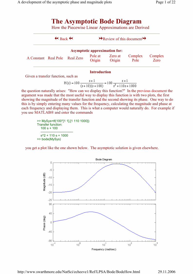
Introduction Given a transfer function, such as

the question naturally arises: "How can we display this function?" In the previous document the argument was made that the most useful way to display this function is with two plots, the first showing the magnitude of the transfer function and the second showing its phase. One way to do this is by simply entering many values for the frequency, calculating the magnitude and phase at each frequency and displaying them. This is what a computer would naturally do. For example if you use MATLAB® and enter the commands

>> MySys=tf(100*[1 1],[1 110 1000]) Transfer function: 100 s + 100 ------------------------------ s^2 + 110 s + 1000 >> bode(MySys)

you get a plot like the one shown below. The asymptotic solution is given elsewhere.

Asymptotic approximation for:

A Constant Real Pole Real Zero Pole at Origin

Zero at Origin

Complex Pole

Complex Zero

of 22A development of the asymptotic phase and magnitude plots

29.11.2006http://www.swarthmore.edu/NatSci/echeeve1/Ref/LPSA/Bode/BodeHow.html

However, there are reasons to develop a method for drawing Bode diagrams manually. By drawing the plots by hand you develop an understanding about how the locations of poles and zeros effect the shape of the plots. With this knowledge you can predict how a system behaves in the frequency domain by simply examining its transfer function. On the other hand, if you know the shape of transfer function that you want, you can use your knowledge of Bode diagrams to generate the transfer function.

The first task when drawing a Bode diagram by hand is to rewrite the transfer function so that

all the poles and zeros are written in the form (1+s/ω0). The reasons for this will become apparent when deriving the rules for a real pole. A derivation will be done using the transfer function from above, but it is also possible to do a more generic derivation. Let's rewrite the transfer function from above.

Now lets examine how we can easily draw the magnitude and phase of this function when s=jω.

First note that this expression is made up of four terms, a constant (0.1), a zero (at s=-1), and

two poles (at s=-10 and s=-100). We can rewrite the function (with s=jω) as four individual phasors.

We will show (below) that drawing the magnitude and phase of each individual phasor is fairly straightforward. The difficulty lies in trying to draw the magnitude and phase of H(jω). We can write H(jω) as a single phasor:

Drawing the phase is fairly simple. We can draw each phase term separately, and then simply add them. The magnitude term is not so straightforward because of the fact that the magnitude terms are multiplied, it would be much easier if they were added - then we could draw each term on a graph and just add them. A method for doing this is outlined below.

The Magnitude Plot

One way to transform multiplication into addition is by using the logarithm. Instead of using a simple logarithm, we will use a deciBel (named for Alexander Graham Bell). {Why the deciBel?} The relationship between a quantity, Q, and its deciBel representation, X, is given by:



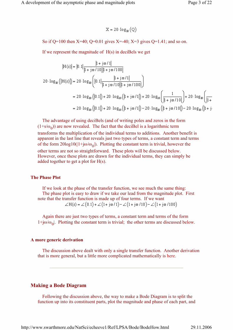
So if Q=100 then X=40; Q=0.01 gives X=-40; X=3 gives Q=1.41; and so on. If we represent the magnitude of H(s) in deciBels we get

The advantage of using deciBels (and of writing poles and zeros in the form

(1+s/ω0)) are now revealed. The fact that the deciBel is a logarithmic term transforms the multiplication of the individual terms to additions. Another benefit is apparent in the last line that reveals just two types of terms, a constant term and terms of the form 20log10(|1+jω/ω0|). Plotting the constant term is trivial, however the other terms are not so straightforward. These plots will be discussed below. However, once these plots are drawn for the individual terms, they can simply be added together to get a plot for H(s).

The Phase Plot

If we look at the phase of the transfer function, we see much the same thing: The phase plot is easy to draw if we take our lead from the magnitude plot. First

note that the transfer function is made up of four terms. If we want

Again there are just two types of terms, a constant term and terms of the form

1+jω/ω0|. Plotting the constant term is trivial; the other terms are discussed below.

A more generic derivation

The discussion above dealt with only a single transfer function. Another derivation that is more general, but a little more complicated mathematically is here.

Making a Bode Diagram

Following the discussion above, the way to make a Bode Diagram is to split the function up into its constituent parts, plot the magnitude and phase of each part, and



then add them up. The following gives a derivation of the plots for each type of constituent part. Examples, including rules for making the plots follow in the next document, which is more of a "How to" description of Bode diagrams.

A Constant Term Consider a constant term,

Magnitude

Clearly the magnitude is constant

Phase

The phase is also constant. If K is positive, the phase is 0° (or any even multiple of 180°). If K is negative the phase is -180°, or any odd multiple of 180°. We will use -180° because that is what MATLAB® uses.

Expressed in radians we can say that if K is positive the phase is 0 radians, if K is

negative the phase is -π radians.

Example

In Brief:

For a constant term, the magnitude plot is a straight line. The phase plot is also a straight line, either at 0° (for a positive constant) or -180° (for a



negative constant).

A Real Pole Consider a simple real pole

The frequency ω0 is called the break frequency, the corner frequency or the 3 dB frequency

(more on this last name later). Magnitude

The magnitude is given by

Let's consider three cases for the value of the frequency:

Case 1) ω<<ω0. This is the low frequency case. We can write an approximation for the magnitude of the transfer function

The low frequency approximation is shown in blue on the diagram

below. Case 2) ω>>ω0. This is the high frequency case. We can write an

approximation for the magnitude of the transfer function

The high frequency approximation is at shown in green on the diagram

below. It is a straight line with a slope of -20 dB/decade going through the break frequency at 0 dB. That is, for every factor of 10 increase in frequency, the magnitude drops by 20 dB.

Case 3) ω=ω0. The break frequency. At this frequency



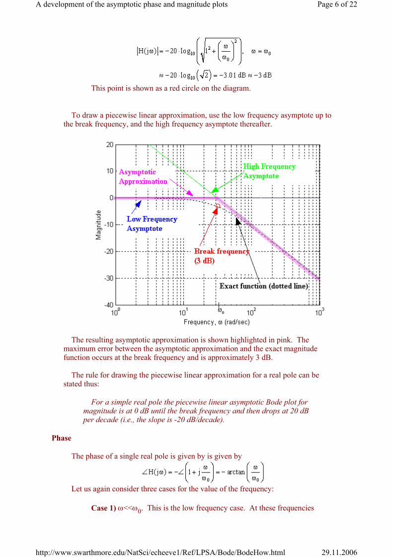
This point is shown as a red circle on the diagram.

To draw a piecewise linear approximation, use the low frequency asymptote up to the break frequency, and the high frequency asymptote thereafter.

The resulting asymptotic approximation is shown highlighted in pink. The maximum error between the asymptotic approximation and the exact magnitude function occurs at the break frequency and is approximately 3 dB.

The rule for drawing the piecewise linear approximation for a real pole can be

stated thus:

For a simple real pole the piecewise linear asymptotic Bode plot for magnitude is at 0 dB until the break frequency and then drops at 20 dB per decade (i.e., the slope is -20 dB/decade).

Phase

The phase of a single real pole is given by is given by

Let us again consider three cases for the value of the frequency:

Case 1) ω<<ω0. This is the low frequency case. At these frequencies



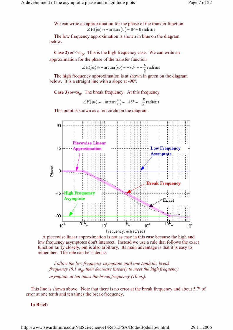
We can write an approximation for the phase of the transfer function

The low frequency approximation is shown in blue on the diagram


approximation for the phase of the transfer function


below. It is a straight line with a slope at -90º. Case 3) ω=ω0. The break frequency. At this frequency

This point is shown as a red circle on the diagram.

A piecewise linear approximation is not as easy in this case because the high and

low frequency asymptotes don't intersect. Instead we use a rule that follows the exact function fairly closely, but is also arbitrary. Its main advantage is that it is easy to remember. The rule can be stated as

Follow the low frequency asymptote until one tenth the break frequency (0.1 ω0) then decrease linearly to meet the high frequency asymptote at ten times the break frequency (10 ω0).

This line is shown above. Note that there is no error at the break frequency and about 5.7º of error at one tenth and ten times the break frequency.

In Brief:



For a simple real pole the piecewise linear asymptotic Bode plot for magnitude is at 0 dB until the break frequency and then drops at 20 dB per decade (i.e., the slope is -20 dB/decade). An nth order pole has a slope of -20*n dB/decade.

The phase plot is at 0 degrees until one tenth the break frequency and then drops linearly to -90 degrees at ten times the break frequency. An nth order pole drops to -90*n degrees.

Examples

Example 1: The first example is a simple pole at 10 radians per second. The low frequency asymptote is the dashed blue line, the exact function is the solid black line, the cyan line represents 0.

Example 2: The second example shows a double pole at 30 radians per second.



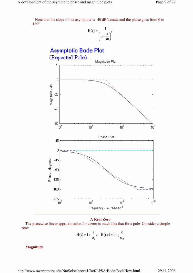
Note that the slope of the asymptote is -40 dB/decade and the phase goes from 0 to -180º.

A Real Zero The piecewise linear approximation for a zero is much like that for a pole Consider a simple

zero:

Magnitude



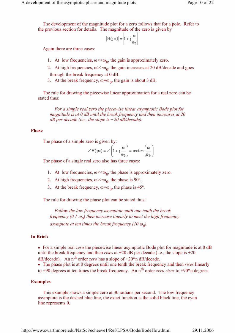
The development of the magnitude plot for a zero follows that for a pole. Refer to the previous section for details. The magnitude of the zero is given by

Again there are three cases:

1. At low frequencies, ω<<ω0, the gain is approximately zero.

2. At high frequencies, ω>>ω0, the gain increases at 20 dB/decade and goes through the break frequency at 0 dB.

3. At the break frequency, ω=ω0, the gain is about 3 dB.

The rule for drawing the piecewise linear approximation for a real zero can be stated thus:

For a simple real zero the piecewise linear asymptotic Bode plot for magnitude is at 0 dB until the break frequency and then increases at 20 dB per decade (i.e., the slope is +20 dB/decade).

Phase

The phase of a simple zero is given by:

The phase of a single real zero also has three cases:

1. At low frequencies, ω<<ω0, the phase is approximately zero.

2. At high frequencies, ω>>ω0, the phase is 90º.

3. At the break frequency, ω=ω0, the phase is 45º.

The rule for drawing the phase plot can be stated thus:

Follow the low frequency asymptote until one tenth the break frequency (0.1 ω0) then increase linearly to meet the high frequency asymptote at ten times the break frequency (10 ω0).

In Brief:

For a simple real zero the piecewise linear asymptotic Bode plot for magnitude is at 0 dB until the break frequency and then rises at +20 dB per decade (i.e., the slope is +20 dB/decade). An nth order zero has a slope of +20*n dB/decade.

The phase plot is at 0 degrees until one tenth the break frequency and then rises linearly to +90 degrees at ten times the break frequency. An nth order zero rises to +90*n degrees.

Examples

This example shows a simple zero at 30 radians per second. The low frequency asymptote is the dashed blue line, the exact function is the solid black line, the cyan line represents 0.



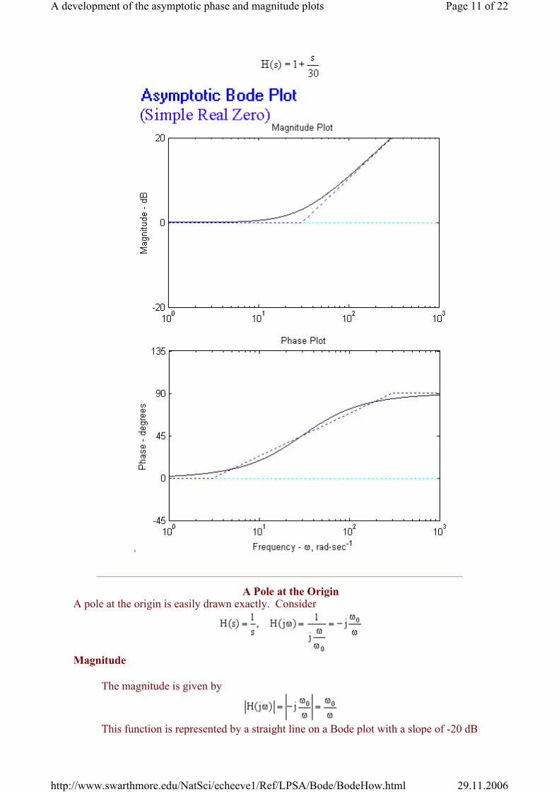
A Pole at the Origin A pole at the origin is easily drawn exactly. Consider

Magnitude


This function is represented by a straight line on a Bode plot with a slope of -20 dB



per decade and going through 0 dB at 1 rad/ sec. It also goes through 20 dB at 0.1 rad/sec, -20 dB at 10 rad/sec...

The rule for drawing the magnitude for a pole at the origin can be thus:

For a pole at the origin draw a line with a slope of -20 dB/decade that goes through 0 dB at 1 rad/sec.

Phase

The phase of a simple zero is given by:

The rule for drawing the phase plot for a pole at the origin an be stated thus:

The phase for a pole at the origin is -90º.

In Brief:

For a simple pole at the origin draw a straight line with a slope of -20 dB per decade and going through 0 dB at 1 rad/ sec. An nth order pole has a slope of -20*n dB/decade.

The phase plot is at -90º degrees. An nth order pole is at -90*n degrees.

Examples

This example shows a simple pole at the origin. The black line is the Bode plot, the cyan line shows zero (dB or degrees).



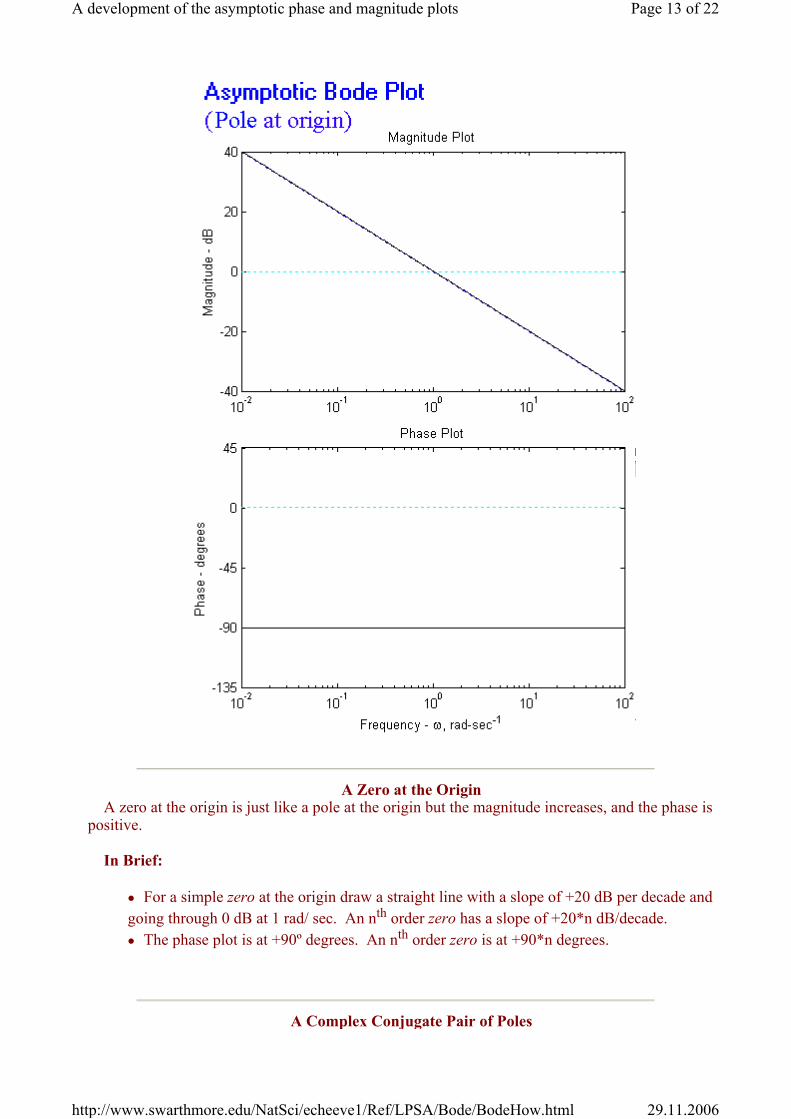
A Zero at the Origin A zero at the origin is just like a pole at the origin but the magnitude increases, and the phase is

positive. In Brief:

For a simple zero at the origin draw a straight line with a slope of +20 dB per decade and going through 0 dB at 1 rad/ sec. An nth order zero has a slope of +20*n dB/decade.

The phase plot is at +90º degrees. An nth order zero is at +90*n degrees.

A Complex Conjugate Pair of Poles



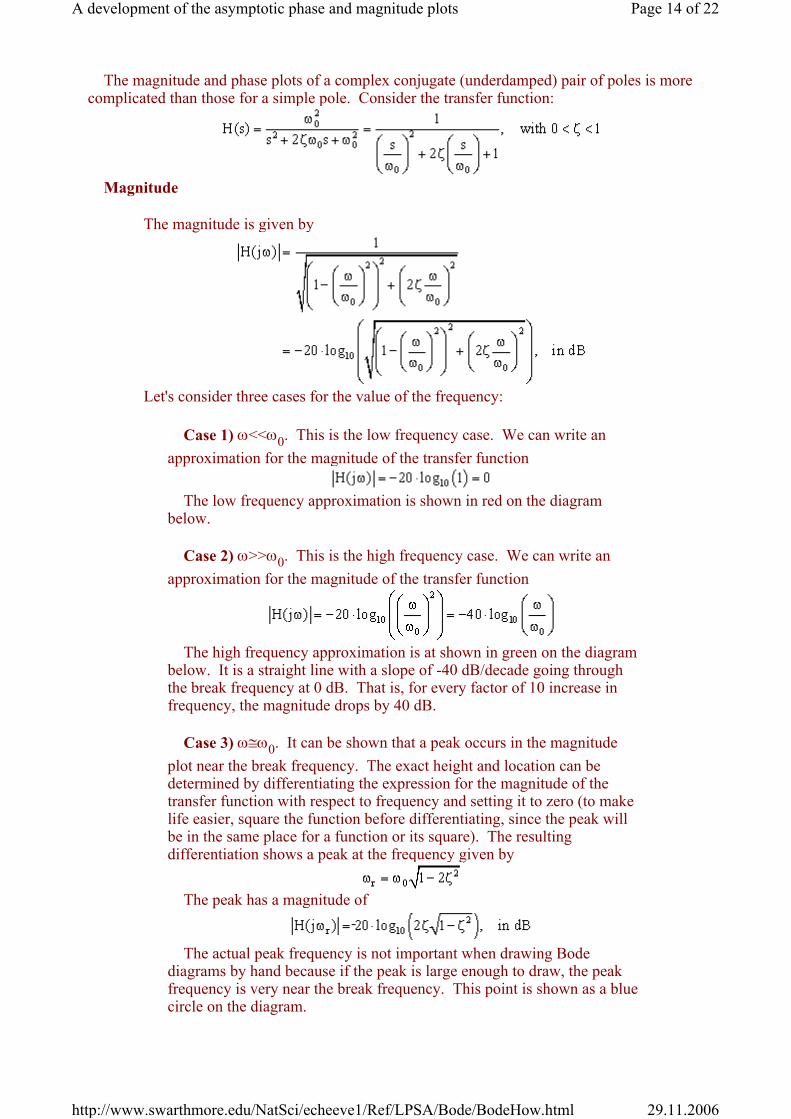
The magnitude and phase plots of a complex conjugate (underdamped) pair of poles is more complicated than those for a simple pole. Consider the transfer function:

Magnitude


Let's consider three cases for the value of the frequency:

Case 1) ω<<ω0. This is the low frequency case. We can write an approximation for the magnitude of the transfer function

The low frequency approximation is shown in red on the diagram


approximation for the magnitude of the transfer function


below. It is a straight line with a slope of -40 dB/decade going through the break frequency at 0 dB. That is, for every factor of 10 increase in frequency, the magnitude drops by 40 dB.

Case 3) ω≅ω0. It can be shown that a peak occurs in the magnitude

plot near the break frequency. The exact height and location can be determined by differentiating the expression for the magnitude of the transfer function with respect to frequency and setting it to zero (to make life easier, square the function before differentiating, since the peak will be in the same place for a function or its square). The resulting differentiation shows a peak at the frequency given by

The peak has a magnitude of

The actual peak frequency is not important when drawing Bode

diagrams by hand because if the peak is large enough to draw, the peak frequency is very near the break frequency. This point is shown as a blue circle on the diagram.



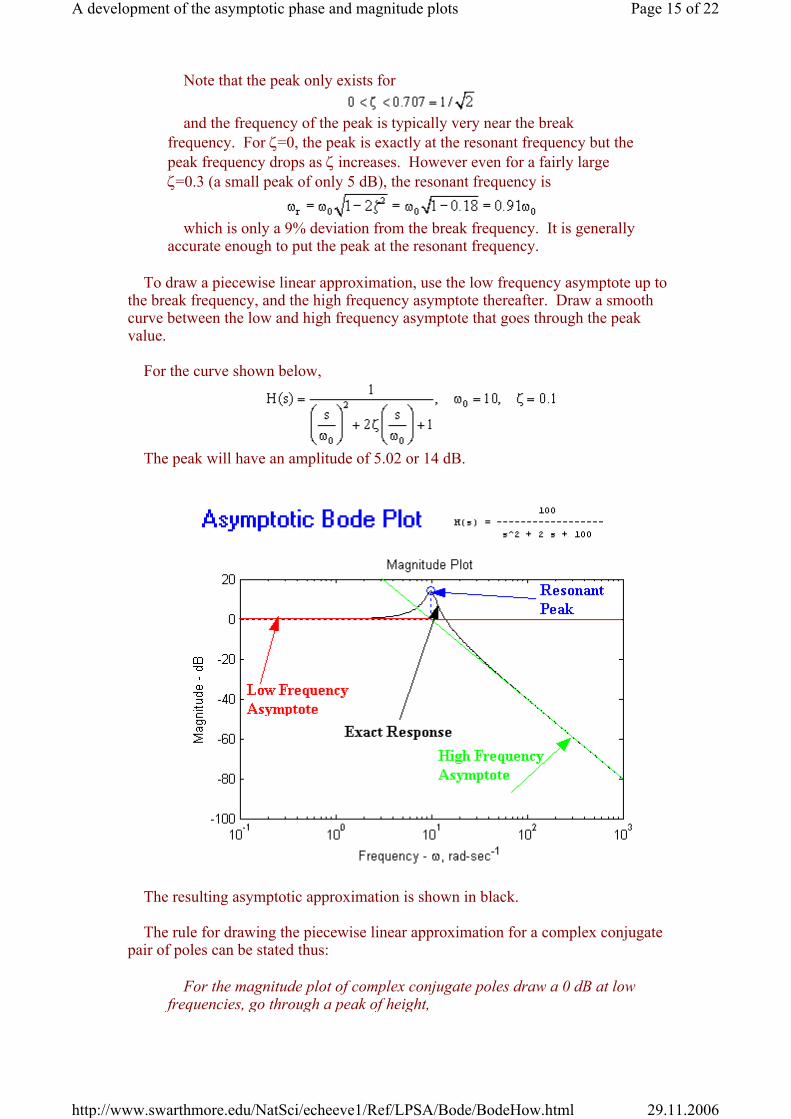
Note that the peak only exists for

and the frequency of the peak is typically very near the break

frequency. For ζ=0, the peak is exactly at the resonant frequency but the peak frequency drops as ζ increases. However even for a fairly large ζ=0.3 (a small peak of only 5 dB), the resonant frequency is

which is only a 9% deviation from the break frequency. It is generally

accurate enough to put the peak at the resonant frequency.

To draw a piecewise linear approximation, use the low frequency asymptote up to the break frequency, and the high frequency asymptote thereafter. Draw a smooth curve between the low and high frequency asymptote that goes through the peak value.

For the curve shown below,

The peak will have an amplitude of 5.02 or 14 dB.

The resulting asymptotic approximation is shown in black. The rule for drawing the piecewise linear approximation for a complex conjugate

pair of poles can be stated thus:

For the magnitude plot of complex conjugate poles draw a 0 dB at low frequencies, go through a peak of height,



. at the break frequency and then drop at 40 dB per decade (i.e., the

slope is -40 dB/decade). The high frequency asymptote goes through the break frequency.

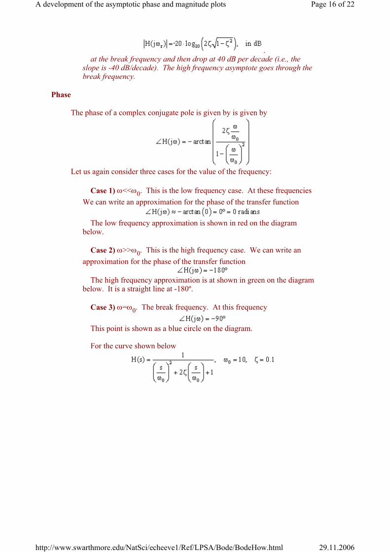
Phase

The phase of a complex conjugate pole is given by is given by

Let us again consider three cases for the value of the frequency:

Case 1) ω<<ω0. This is the low frequency case. At these frequencies We can write an approximation for the phase of the transfer function

The low frequency approximation is shown in red on the diagram


approximation for the phase of the transfer function

The high frequency approximation is at shown in green on the diagram below. It is a straight line at -180º.

Case 3) ω=ω0. The break frequency. At this frequency

This point is shown as a blue circle on the diagram. For the curve shown below



A piecewise linear approximation is not easy in this case, and there are no hard and

fast rules for drawing it. The most common way is to look up a graph in a textbook with a chart that shows phase plots for many values of ζ. Another way is to use connect the low frequency asymptote to the high frequency asymptote starting at

and ending at

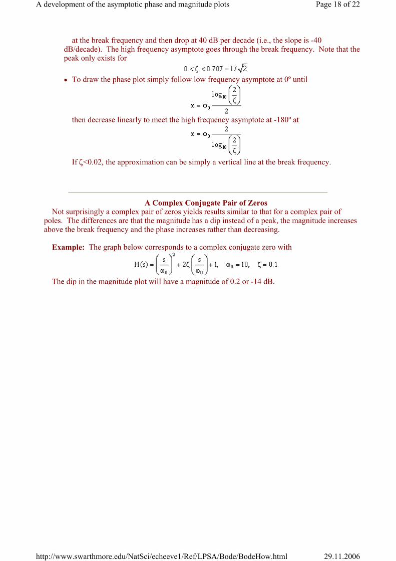
If ζ<0.02, the approximation can be simply a vertical line at the break frequency. The rule for drawing phase of an underdamped pair of poles can be stated as

Follow the low frequency asymptote at 0º until

then decrease linearly to meet the high frequency asymptote at -180º

at

In Brief:

For the magnitude plot of complex conjugate poles draw a 0 dB at low frequencies, go through a peak of height,

.



at the break frequency and then drop at 40 dB per decade (i.e., the slope is -40 dB/decade). The high frequency asymptote goes through the break frequency. Note that the peak only exists for

To draw the phase plot simply follow low frequency asymptote at 0º until

then decrease linearly to meet the high frequency asymptote at -180º at

If ζ<0.02, the approximation can be simply a vertical line at the break frequency.

A Complex Conjugate Pair of Zeros Not surprisingly a complex pair of zeros yields results similar to that for a complex pair of

poles. The differences are that the magnitude has a dip instead of a peak, the magnitude increases above the break frequency and the phase increases rather than decreasing.

Example: The graph below corresponds to a complex conjugate zero with

The dip in the magnitude plot will have a magnitude of 0.2 or -14 dB.



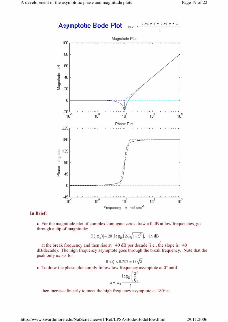
In Brief:

For the magnitude plot of complex conjugate zeros draw a 0 dB at low frequencies, go through a dip of magnitude:

. at the break frequency and then rise at +40 dB per decade (i.e., the slope is +40

dB/decade). The high frequency asymptote goes through the break frequency. Note that the peak only exists for

To draw the phase plot simply follow low frequency asymptote at 0º until

then increase linearly to meet the high frequency asymptote at 180º at



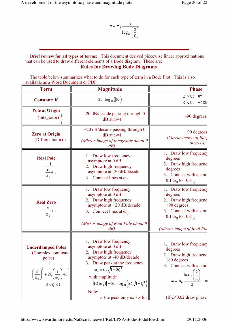
Brief review for all types of terms: This document derived piecewise linear approximations that can be used to draw different elements of a Bode diagram. These are:

Rules for Drawing Bode Diagrams

The table below summarizes what to do for each type of term in a Bode Plot. This is also available as a Word Document or PDF

Term Magnitude Phase

Constant: K

Pole at Origin (Integrator)

-20 dB/decade passing through 0 dB at ω=1

-90 degrees

Zero at Origin (Differentiator)

+20 dB/decade passing through 0 dB at ω=1

(Mirror image of Integrator about 0 dB)

+90 degrees (Mirror image of Integ

degrees)

Real Pole

1. Draw low frequency asymptote at 0 dB

2. Draw high frequency asymptote at -20 dB/decade

3. Connect lines at ω0.

1. Draw low frequencydegrees

2. Draw high frequencdegrees

3. Connect with a strai0.1·ω0 to 10·ω0

Real Zero


2. Draw high frequency asymptote at +20 dB/decade

3. Connect lines at ω0.

(Mirror image of Real Pole about 0 dB)


2. Draw high frequenc+90 degrees

3. Connect with a strai0.1·ω0 to 10·ω0

(Mirror image of Real Pol

Underdamped Poles (Complex conjugate

poles)



3. Draw peak at the frequency

with amplitude

Note:

the peak only exists for


2. Draw high frequenc180 degrees

3. Connect with a strai

(If ζ<0.02 draw phase



For multiple order poles and zeros, simply multiply the slope of the magnitude plot by the order of the pole (or zero) and multiply the high and low frequency asymptotes of the phase by the order of the system.

For example:

This page is modeled after the one at http://lims.mech.nwu.edu/~lynch/courses/ME391/2002/bodesketching.pdf

Back to Bode Plot Page

© Copyright 2005 Erik Cheever This page may be freely used for educational purposes. Comments? Questions? Suggestions?

Erik Cheever Department of Engineering Swarthmore College

the peak frequency is

typically very near ω0.

4. Connect lines

to -180 degrees at ω

You can also look in a textexamples

Underdamped Zeros (Complex conjugate

zeros)


2. Draw high frequency asymptote at +40 dB/decade

3. Draw a dip in the response at frequency

with amplitude

Note:

the dip only exists for

the dip frequency is

typically very near ω0.

4. Connect lines

(Mirror image of Underdamped Pole about 0 dB)


2. Draw high frequenc+180 degrees

3. Connect with a strai

(If ζ<0.02 draw phase to +180 degrees at ω0)

You can also look in a textexamples

(Mirror image of Underda0 degrees)

Second Order Real Pole



3. Connect lines at break frequency.

-40 db/dec is used because of order of pole=2. For a third order pole, asymptote is -60 db/dec

1. Draw low frequency asymptote at 0 degrees

2. Draw high frequency asymptote at -180 degrees

3. Connect with a straight line from 0.1·ω0 to 10·ω0

-180 degrees is used because order of pole=2. For a third order pole, high frequency asymptote is at -270 degrees.



Back Rules for drawing Bode diagrams

© Copyright 2005 Erik Cheever This page may be freely used for educational purposes. Comments? Questions? Suggestions?

Erik Cheever Department of Engineering Swarthmore College



the asymptotic bode diagram - miun.seapachepersonal.miun.se/~amiyou/ae/bodeplots.pdf · the...

Documents