the impact of banning juvenile gun possession

691

[Journal of Law and Economics, vol. XLIV (October 2001)]� 2001 by The University of Chicago. All rights reserved. 0022-2186/2001/4402-0015$01.50

THE IMPACT OF BANNING JUVENILEGUN POSSESSION

THOMAS B. MARVELLJustec Research

Abstract

A 1994 federal law bans possession of handguns by persons under 18 years ofage. Also in 1994, 11 states passed their own juvenile gun possession bans. Eighteenstates had previously passed bans, 15 of them between 1975 and 1993. These lawswere intended to reduce homicides, but arguments can be made that they have noeffect on or that they even increase the homicide rate. This paper estimates the laws’impacts on various crime measures, primarily juvenile gun homicide victimizationsand suicide, using a fixed-effects research design with state-level data for at least 19years. The analysis compares impacts on gun versus nongun homicides and gunversus nongun suicides. Even with many different crime measures and regressionspecifications, there is scant evidence that the laws have the intended effect of re-ducing gun homicides.

I. Introduction

Guns are the second leading cause of death in the United States amongyouths ages 10–24, and the firearm death rate for U.S. minors is 12 timesthe average for other industrialized countries.1 Gun murders of and by ju-veniles roughly doubled between 1985 and 1992, while the number of nongunmurders remained stable.2 Consequently, governments have attempted to getguns out of the hands of juveniles. The federal government and probably allstates have long prohibited gun sales to minors.3 Later laws, the subject ofthis study, go further and prohibit possession of guns by juveniles (aimedat, presumably, guns that were originally purchased by adults). States passedsuch laws with increasing frequency in the 1980s and early 1990s, and TitleXI of the Federal Crime Control and Law Enforcement Act of 1994 madethe ban effective nationwide on September 13, 1994.

Table 1 lists 34 state laws that ban juvenile gun possession, along withtheir effective dates (the laws only apply to violations on or after the

1 Susan DeFrancesco, Children and Guns, 29 Pace L. Rev. 275 (1999).2 James A. Fox & Marianne W. Zawitz, Homicide Trends in the United States (2000).3 Jens Ludwig, Concealed-Gun-Carrying Laws and Violent Crime: Evidence from State Panel

Data, 18 Int’l Rev. L. & Econ. 239 (1998).

692 the journal of law and economics

TABLE 1

Laws Banning Juvenile Handgun Possesson

Under Age of Brief Citation Effective Date

Federal 18 18-922(x) September 13, 1994Alaskaa 16 11.61.220 January 1, 1980Arizonaa,b 18 13-3111 July 18, 1993Arkansasa,b 18 5-73-119 July 4, 1989Californiaa 18 Penal 12101 January 1, 1989Coloradoa 18 18-12-108.5 September 13, 1993Delaware 18 11-1448 July 15, 1994Florida 18 790.22 January 1, 1994Georgiab 18 16-11-132 July 1, 1994Idahob 18 18-3302F July 1, 1994Illinois 18 720-5/24-3 pre-1970Indiana 18 35-47-10-5 July 1, 1994Kansasb 18 21-4204a July 1, 1994Kentuckyb 18 527.100 July 15, 1994Michigana 18 750.234f March 28, 1991Minnesotaa 18 624.713 August 1, 1975Mississippib 18 97-37-14 July 1, 1994Nebraskaa 18 28-1204 July 1, 1978Nevadab,c 18 202.300 July 1, 1995New Jerseya 18 2C:58-6.1 June 27, 1980New Yorka 16 265.05 September 1, 1974North Carolinaa,b 18 14-269.7 September 1, 1993North Dakotaa,b 18 62.1-02-01 July 1, 1985Oklahomaa,b 18 21-1273 June 7, 1993Oregona 18 166.250 January 1, 1990Rhode Islandb 15 11-47-33 pre-1970South Carolinab 21 16-23-30 pre-1970South Dakotab 18 23-7-44 July 1, 1994Tennessee 18 39-17-1319 July 1, 1994Utaha 18 76-10-509 October 21, 1993Vermontb 16 13-4008 pre-1970Virginiaa 18 18.2-308.7 July 1, 1993Washingtonb 21 9.41.040 July 1, 1994West Virginiaa,b 18 61-7-8 July 9, 1989Wisconsin 18 948.60 pre-1970

Note.—Sixteen states do not have bans. Ten are Brady Act states (Alabama, Louisiana, Maine, Montana,New Hampshire, New Mexico, Ohio, Pennsylvania, Texas, and Wyoming), and six are non–Brady Actstates (Connecticut, Hawaii, Iowa, Maryland, Massachusetts, and Missouri).

a States with laws effective 1974–93.b Brady Act states. (Federal waiting periods and background checks apply in 1994 because these states

did not have preexisting laws.)c A pre-1970 Nevada law applied to persons under 14.

effective dates). This information was obtained through research into statestatutory compilations and session laws, and it was checked against twoother surveys.4

4 Gwen A. Holden,et al., Compilation of State Firearm Codes that Affect Juveniles (1994);Bureau of Alcohol, Tobacco and Firearms, Firearms State Laws and Published Ordinances(20th ed. 1994) (hereafter referred to as ATF).

juvenile gun possession 693

The federal law, as well as the typical state law, makes it a misdemeanorfor a person under 18 (21 in two states) to possess a handgun, with severalexceptions, such as hunting or target shooting with the permission of a parent.Many state laws also ban possession of rifles and other deadly weapons byjuveniles. As of 1994, five state bans applied only to persons younger than15 or 16 (Table 1). These are not counted as juvenile gun ban laws for thepurpose of this study because children that young seldom commit homicide.5

Among the states that did not enact juvenile gun possession bans, Massa-chusetts and New York have strict general gun possession laws,6 and law-makers there might have believed that special laws for juveniles were un-necessary. The federal law also makes it illegal for a person to provide aminor with a handgun. Most states have similar laws, some enacted with thepossession ban and some before the ban.

The issue addressed in this article is whether the juvenile gun possessionbans have the effect of reducing gun homicides, especially of juveniles. Theassumption behind the laws is that the bans reduce the number of juvenileswho have guns and, thus, the number who use guns.7 The impact on crimemight be limited because existing laws prohibited juveniles from purchasingguns, carrying concealed handguns, and possessing guns if they have beenconvicted of a felony.8 Thus, the question is whether crime rates are affectedby a change from a situation where juveniles can possess guns, but cannotlegally purchase or conceal them, to a situation where they can possess gunsonly with adult monitoring. Perhaps the major practical impact is creatingdisincentives to keeping guns at home. The laws might add an additionalincentive for juveniles not to carry concealed weapons or purchase weaponssince it adds a second charge when prosecuted, a charge that can be pros-ecuted in federal court.

An initial consideration is whether the bans increase the expected cost tojuveniles for possessing guns, which largely determines whether the ban canhave any effect.9 The costs include confiscation of the weapon, informalsanctions applied by such persons as relatives, juvenile officers, and prose-

5 See Terry Allen & Glen Buckner, A Graphical Approach to Analyzing Relationships be-tween Offenders and Victims UsingSupplementary Homicide Reports, 1 Homicide Stud. 129(1997); and Michael D. Maltz, Visualizing Homicide: A Research Note, 14 J. QuantitativeCriminology 397 (1998).

6 ATF, supra note 4.7 There apparently is no statement that this is the actual intent of juvenile gun bans. The

legislative history of the federal ban consists of justifications for federal action under theCommerce Clause of the U.S. Constitution; that is, guns and drug markets are interrelated andcross state lines. See Steven Rosenberg, Just Another Kid with a Gun?United States v. MichaelR.: Reviewing the Youth Handgun Safety Act under theUnited States v. Lopez CommerceClause Analysis, 28 Golden Gate Univ. L. Rev. 51 (1998).

8 ATF, supra note 4.9 See Philip J. Cook & James A. Leitzel, “Perversity, Futility, Jeopardy”: An Economic

Analysis of the Attack on Gun Control, 59 Law & Contemp. Probs. 91 (1996).


cutors, and conviction and sentencing by courts. These costs are more likelyto occur with greater efforts to uncover and report juveniles’ gun possession.Information on all these topics is lacking, so it is impossible at this point tohypothesize whether the laws have much impact.

Assuming that possession actually entails a cost, there are many mecha-nisms by which the bans might affect the actual use of guns and, thus, crimerates. The most obvious is that juveniles who do not possess guns are lesslikely to carry guns and thus less likely to use them during crimes or alter-cations. If they do not possess guns, juveniles are less likely to retrieve themin the middle of a dispute or to use them later in retaliation. The bans candisrupt gun markets among juveniles because the law increases the costs ofcarrying gun inventories.

On the other hand, the gun bans might increase crime against young personsbecause criminals might consider them less risky targets.10 A criminal con-templating robbery or assault probably takes into consideration the likelihoodthat potential victims are armed and likely to defend themselves. If thepotential victim appears to be under 18 years old, after a ban goes into effect,an aggressor might believe that armed resistance is less likely because of thejuvenile gun possession ban. As discussed earlier, the possession bans do notmake it any more illegal to carry a concealed handgun, but, again, the juvenileis less likely to have a handgun available if possession is less likely. Theban also can make aggression more likely because the aggressor is lessconcerned that the victim will retaliate by retrieving a gun.

An additional indicator of the impact of the juvenile gun possession bansis whether they reduce gun suicide by juveniles. There is a close relationshipover time between the percentages of juvenile suicides and homicides bygun.11 One would expect that the choice of whether to use a gun in suicidedepends largely on whether a gun is readily available. Although possessionis only one of several factors suggesting availability, if the laws reducepossession, they should reduce gun suicides.

Preliminary indications of the likely impact can be seen in trends for gunhomicide victimization for persons 15–19 years old, which is a group likelyto be affected by the ban if it has an impact. Figure 1 plots the trends forthe percentage of homicide victims who were killed by guns (since thenumber of nongun homicides changed little over time, the lines in Figure 1also approximate trends in the number of gun homicides). This percentagerose from about 65 percent in the first half of the 1980s to 86 percent in1992, leveled off for 2 years, and then declined modestly. The leveling offoccurred when more and more states were enacting juvenile gun possession

10 For example, John R. Lott, Jr., & David B. Mustard, Crime, Deterrence, and Right-to-Carry Concealed Handguns, 26 J. Legal Stud. 1 (1997).

11 Alfred Blumstein & Daniel Cork, Linking Gun Availability to Youth Gun Violence, 59Law & Contemp. Probs. 5 (1996).


Figure 1.—Percent of homicides with guns

bans, and the decline occurred right after the substantial lawmaking activityin 1994, when most states first became covered by the ban (Table 1). At firstglance, the trends suggest that the laws have the desired effect of reducinggun homicides. However, this impression disappears when one looks at trendsin adult crimes; the post-1994 drop in percentage of homicides with gunsoccurred here as well. The initial impression from Figure 1 that the lawsreduce gun homicide is probably only a reflection of general trends inhomicides.12

The purpose of this paper is to explore this relationship with more elaboratedata and analysis than are illustrated in Figure 1. The next section describesthe methodology, which is a state-level multiple time-series regression that

12 Commentators have given many reasons for the decline in murder and other crimes in the1990s. I argue that it is due to the incapacitation impact of rising prison populations and theslackening of the crack era. Thomas B. Marvell & Carlisle E. Moody, The Impact of Out-of-State Prison Population on State Homicide Rates: Displacement and Free-Rider Effects, 36Criminology 513 (1998); Thomas B. Marvell & Carlisle E. Moody, Female and Male HomicideVictimization Rates: Comparing Trends and Regressors, 37 Criminology 879 (1999). Othersuggested causes include the legalization of abortion in the 1970s (John J. Donohue III &Steven D. Levitt, The Impact of Legalized Abortion on Crime, 116 Q. J. Econ. 379 (2001))and better police practices (Malcolm Gladwell, The Tipping Point: How Little Things CanMake a Big Difference (2000)).


compares the impacts of the laws on different homicide categories. The thirdsection describes the variables, and the fourth gives the results, which arethat there is no evidence that the juvenile gun possession bans, taken as awhole, reduce gun homicides or total homicides.

II. Methodology

The multiple time-series regression has become a common tool to estimatethe impact of legal changes, and the methods are continually improving.13

The regressions here encompass 45–50 states and 18–29 years, dependingon the dependent variable, using the standard fixed-effects procedure. Theregressions are weighted by population when the dependent variable is hom-icide and by lesser amounts (varying from population to the .3 power topopulation to the .7 power) for other crimes as determined by the Bruesch-Pagan test.14 Weighting is necessary because crime rates vary over time morein small states, and weights are greater in homicide equations because hom-icides are less frequent events; so the discrepancy between variation in smalland large states is especially large. The data start in 1970 because severalcontrol variables lack data for earlier years. The last year with available datais 1998 or 1999, depending on the series. The analysis, therefore, includesat least 4 full years of experience under each law. The main dependentvariables are homicide victimizations for various age groups, and I use asizeable number of other crime measures for robustness checks. The gunpossession bans are represented by dummy variables.

The basic procedure is strengthened by comparing the estimated impactsof the laws on crimes that one would expect to be affected the most by thelaws to the impacts on crimes less likely to be affected. The analysis, forexample, compares the coefficients on the law dummies when gun homicidesare the dependent variable with coefficients with nongun homicides. Thishelps control for missing variables that are not otherwise controlled for bythe elaborate control mechanism possible with the multiple time-series design,as discussed below. The comparison is done with the STEST option in theSYSLIN procedure in SAS,15 which tests whether differences between co-

13 For example, Lott & Mustard,supra note 10; Thomas B. Marvell & Carlisle E. Moody,Determinate Sentencing and Abolishing Parole: The Long-Term Impacts on Prisons and Crime,34 Criminology 107 (1996).

14 William H. Greene, Econometric Analysis 394–95 (2d ed. 1993).15 SAS Institute, SAS/ETS User’s Guide, Version 6 (2d ed. 1993). Using the multiple time-

series procedure with dummy variables to evaluate the impact of laws or other impacts is thesame as the difference-on-difference procedure (Jeffrey M. Wooldridge, Introductory Econom-ics: A Modern Approach (2000)), but it has the benefit that one can set dummies at the effectivedate of each law that went into effect during the period when data are available, as opposedto setting a uniform date for all laws. Also, using anF-test to compare coefficients is animprovement on the difference-on-difference-on-difference procedure, whereby the impact ofthe law change on a crime type that is expected to be affected by the law is compared withthe impact on a crime having no expected impact (for example, Ludwig,supra note 3). The


efficients on an independent variable used in separate regressions are statis-tically significant.

III. Dependent Variables16

Most dependent variables are gun homicide victimization rates for variousage groups and homicide offending rates by juveniles. When juveniles com-mit homicide, the victims are overwhelmingly persons of the same age orslightly older,17 so measures of gun homicide victimization are for personsin their late teens and early twenties. Alternate specifications use measuresof juvenile homicide offending and general crime rate variables. All crimesare expressed as rates, divided by 100,000 persons in the age group inquestion. The numerous variables are best described in outline form.

A. Victimization (Homicide and Suicide)

1. The primary victimization data are from the Centers for Disease Controland Prevention Internet site, where state-level mortality data are availablefor 1979–98. In addition, earlier total homicide and gun homicide datawere obtained from published mortality tables.18 The four types of data,and the years available, are the following:a. Gun and nongun homicide victims, ages 15–19 (1979–98).b. Gun and nongun homicide victims, ages 15–24 (1979–98).c. Gun and nongun homicide victims of all ages (1968–98).d. Gun and nongun suicide victims, ages 15-19 (1979–98).

2. Additional juvenile victimization data, compiled by James A. Fox inJanuary 2001, were obtained from the Bureau of Justice Statistics (BJS)Internet site. Data are not used for five states for which observations aremissing for more than 2 years (Florida, Iowa, Kansas, Maine, and Mon-tana):a. Homicide victims, ages 14–17 (1976–99).b. Homicide victims, ages 14–24 (1976–99).

separate regressions mean that the two types of crime are allowed to have their own coefficientson the control variables, and again we need not set law dummies at the same year.

16 The data set and basic programs used here are available from the author at [email protected] at http://www.mmarvell.com/justec.html.

17 Allen & Buckner, supra note 5; Maltz,supra note 5.18 Data are from National Center for Health Statistics, Vital Statistics of the United States

1978 (1982), and earlier versions. All the homicide data exclude legal homicides (executionsand police killings).


B. Offending and Reported Crime

Homicide arrests for the following two categories were also prepared byJames A. Fox and placed on the BJS Internet site:1. Homicide offending ages 14–17 (1976–99).2. Homicide offending ages 14–24 (1976–99).

Finally, we use the seven Uniform Crime Report (UCR) categories (hom-icide, rape, robbery, assault, burglary, larceny, and auto theft) with data from1968–99.

C. Issues Pertaining to Homicide and Suicide Data

Small states often have no juvenile homicides in any given year. Becausethis theoretically creates problems with regression analysis, I have droppedstates from a given analysis if the dependent variable is zero for more than2 years. The states that were dropped, which number up to 16, are listed inthe tables along with the regression results. In the parallel SYSLIN regres-sions, the state is dropped when data are missing for either dependent variable.For the remaining zero values (that is, one or two such zeros in a state), thenumber of homicides is set at .1 before logging (or for the Fox data sets,the homicide rate is set at .1). Coefficients on aggregate law variables changelittle when all states are included (because the regressions are weighted bypopulation), but coefficients for individual state law dummies are erratic instates with many zero homicide years.

The juvenile homicide offending rates, because they are based on arrests,are probably overstated in relation to victimization rates and offending ratesfor older age groups because juveniles are less likely to escape arrest.19

We have no measure of gun homicides committed by juveniles, althoughthat is the immediate target of the law, because data at the state level arevery incomplete and erratic. As a practical matter, however, the measure oftotal juvenile homicide offending serves nearly the same purpose becausethe variation in homicide rates is largely due to variations in gun homiciderates.20 Also, for policy purposes, victimization is more important than of-fending because the overriding purpose of the laws is to reduce harm, andany impact on offending is simply the means to achieve that purpose.

19 Howard N. Snyder, The Overrepresentation of Juvenile Crime Proportions in RobberyClearance Statistics, 15 J. Quantitative Criminology 151 (1999); Thomas B. Marvell & CarlisleE. Moody, Age Structure and Crime Rates: The Conflicting Evidence, 7 J. Quantitative Crim-inology 237 (1991).

20 Fox & Zawitz, supra note 2.


IV. Independent Variables

A. Juvenile Gun Bans

The key independent variables, of course, are those representing laws thatban juvenile gun possession, as listed in Table 1. After the year the law wentinto effect, the law variable is one. During that year, it is a decimal repre-senting the portion of the year the law was in effect. The states are dividedinto three groups (Table 1): (1) 15 states that passed laws in 1975–93, (2)11 states that passed laws in 1994, and (3) 21 states without laws by 1994(the remaining three states had laws before 1970).21 Again, laws banningpossession only for those under 15 or 16 are ignored. In the second group,the state laws went into effect only a few months before the federal law, sothat dummy variables cannot separate their impact from that of the federallaw. The main difference between the second and third groups is that thelatter is affected only by the federal law, typically enforced only in the federalcourts, whereas in the second group enforcement is possible in both stateand federal courts. These 11 states received a double dose of law, althoughlargely redundant (state authorities can enforce the federal law, and it isunlikely that federal prosecutors indict many juveniles for gun possession).

Homicides in the second and third groups of states, where dummy variablesbegin in 1994, are also subject to the changes made by other federal laws thatyear. The most important are waiting periods and background checks for firearmpurchases, required under the Brady Act, beginning February 28, 1994. Theact is applicable to the majority of states that did not already require waitingperiods.22 These states are indicated in Table 1, and dummies representing theBrady Act for these states are included in later regressions. Also, the CrimeControl and Law Enforcement Act of 1994 contains several major crime-reduction programs such as truth in sentencing, enhanced penalties for drugoffenses and using firearms in crimes, and funds for hiring new police andadvancing community policing. These nationwide events are controlled for byentering year effects and by comparing gun and nongun crime regressions.

B. Other Independent Variables

Additional independent variables are those typically used in other state-level studies of crime.23 These studies explain the theoretical importance of

21 The fact that most law dummies are for the same year suggests that clustering effectsmight bias thet-ratios. To test for these, I used the ACOV option in SAS PROC REG, withthe TEST statement for the law dummies. The resulting significance levels for the law dummiesare very close to those for the originalt-ratios.

22 ATF, supra note 4.23 See Thomas B. Marvell & Carlisle E. Moody, The Lethal Effects of Three-Strikes Laws,

30 J. Legal Stud. 89 (2001).


the variables and describe the sources of data. Age structure variables arecensus data for the percent population of persons ages 15–17, 18–24, 25–29,and 30–34, the ages with highest arrest rates. Economic variables are theunemployment rate, the number employed, real welfare payments, real per-sonal income, and the poverty rate. Economic downturns might increaseviolent crime by increasing strain or might reduce it by reducing interactionamong potential aggressors and victims. Prison population is the number ofprisoners sentenced to more than 1 year, and it is the average of the currentand prior year-end figures. All these variables are per capita and logged.

In addition, I make full use of the unique ability of the multiple time-series design to control for missing variables—variables that are not knownor that lack adequate data. State dummies control for such factors that causecrime rates to differ generally from one state to another. Year dummies controlfor missing variables that cause crime rates to rise or fall nationwide in ayear. Separate linear trend variables for each state control for factors thatcause trends in the state to differ from nationwide trends. Without them,coefficients on the law dummies are likely to be dominated by such trenddifferences, as opposed to any changes that took place at the time the lawwent into effect. Finally, lagged dependent variables reduce autocorrelationand further mitigate missing-variable bias. Two lags are entered when thedependent variables are UCR crimes and total gun and nongun victimizationbecause data start before 1970. The remaining regressions have one laggeddependent variable and lose 1 year of data.

V. Results

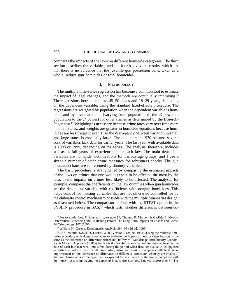
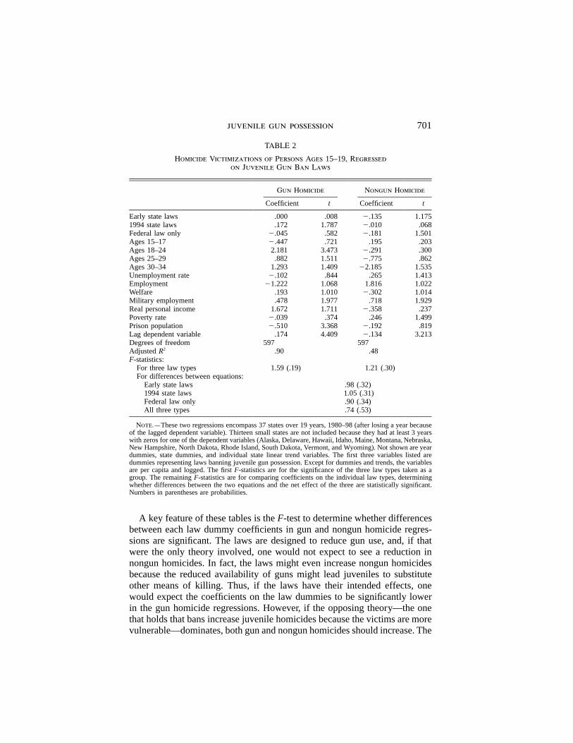
The most important regressions are in Tables 2, 3, and 4, where dependentvariables are homicide victimization rates for persons 15–19 years old, per-sons 15–24 years old, and all persons, respectively. For each table, there aretwo regressions, one with gun and one with nongun homicides. The coef-ficients for the early state laws are very small and not significant throughoutexcept for the negative estimate for nongun total homicides (Table 4). Onthe one hand, the coefficients on the 1994 state law dummies are positivein the three gun homicide regressions, but only significant to the .10 level.On the other hand, the elasticities of up to .17 are fairly sizeable, and theirdecline as the age bracket expands is consistent with the suggestion that the1994 state laws increase juvenile homicide. The 1994 state law dummy hasno noticeable impact on nongun homicides. Finally, all coefficients on the“federal law only” dummies are negative, but significant to the .05 level onlyfor gun homicides of all ages (Table 4), which is due solely to New York,a topic discussed later. As might be expected, in a separate analysis in whichthe 1994 state law variable and the federal law variable are combined intoone variable, it is everywhere far from significant. The same result also occurswhen the three law variables are combined into a single variable.


TABLE 2

Homicide Victimizations of Persons Ages 15–19, Regressedon Juvenile Gun Ban Laws

Gun Homicide Nongun Homicide

Coefficient t Coefficient t

Early state laws .000 .008 �.135 1.1751994 state laws .172 1.787 �.010 .068Federal law only �.045 .582 �.181 1.501Ages 15–17 �.447 .721 .195 .203Ages 18–24 2.181 3.473 �.291 .300Ages 25–29 .882 1.511 �.775 .862Ages 30–34 1.293 1.409 �2.185 1.535Unemployment rate �.102 .844 .265 1.413Employment �1.222 1.068 1.816 1.022Welfare .193 1.010 �.302 1.014Military employment .478 1.977 .718 1.929Real personal income 1.672 1.711 �.358 .237Poverty rate �.039 .374 .246 1.499Prison population �.510 3.368 �.192 .819Lag dependent variable .174 4.409 �.134 3.213Degrees of freedom 597 597AdjustedR2 .90 .48F-statistics:

For three law types 1.59 (.19) 1.21 (.30)For differences between equations:

Early state laws .98 (.32)1994 state laws 1.05 (.31)Federal law only .90 (.34)All three types .74 (.53)

Note.—These two regressions encompass 37 states over 19 years, 1980–98 (after losing a year becauseof the lagged dependent variable). Thirteen small states are not included because they had at least 3 yearswith zeros for one of the dependent variables (Alaska, Delaware, Hawaii, Idaho, Maine, Montana, Nebraska,New Hampshire, North Dakota, Rhode Island, South Dakota, Vermont, and Wyoming). Not shown are yeardummies, state dummies, and individual state linear trend variables. The first three variables listed aredummies representing laws banning juvenile gun possession. Except for dummies and trends, the variablesare per capita and logged. The firstF-statistics are for the significance of the three law types taken as agroup. The remainingF-statistics are for comparing coefficients on the individual law types, determiningwhether differences between the two equations and the net effect of the three are statistically significant.Numbers in parentheses are probabilities.

A key feature of these tables is theF-test to determine whether differencesbetween each law dummy coefficients in gun and nongun homicide regres-sions are significant. The laws are designed to reduce gun use, and, if thatwere the only theory involved, one would not expect to see a reduction innongun homicides. In fact, the laws might even increase nongun homicidesbecause the reduced availability of guns might lead juveniles to substituteother means of killing. Thus, if the laws have their intended effects, onewould expect the coefficients on the law dummies to be significantly lowerin the gun homicide regressions. However, if the opposing theory—the onethat holds that bans increase juvenile homicides because the victims are morevulnerable—dominates, both gun and nongun homicides should increase. The


TABLE 3

Homicide Victimizations of Persons Ages 15–24, Regressedon Juvenile Gun Ban Laws



Early state laws �.000 .007 .007 .1181994 state laws .129 1.757 .124 1.450Federal law only �.079 1.324 �.052 .748Ages 15–17 .195 .419 .140 .259Ages 18–24 1.098 2.524 �.136 .271Ages 25– 29 1.208 2.826 �.101 .207Ages 30–34 .462 .682 �1.050 1.330Unemployment rate .018 .202 .135 1.295Employment �.336 .388 �.221 .219Welfare .121 .831 .027 .162Military employment .350 1.913 .065 .310Real personal income 1.366 1.901 .811 .970Poverty rate .007 .089 .097 1.047Prison population �.449 3.898 �.200 1.497Lag dependent variable .211 6.005 �.100 2.749Degrees of freedom 750 750AdjustedR2 .91 .72F-statistics:


Early state laws .01 (.92)1994 state laws .00 (.96)Federal law only .09 (.77)All three types .04 (.99)

Note.—See note to Table 2. The regressions encompass 46 states over 19 years, 1980–98. Four smallstates are excluded (New Hampshire, North Dakota, Vermont, and Wyoming).

increase might be greater for nongun homicides, because if the attacker nolonger fears the victim has a gun, he or she is less likely to rely on thequickest and most lethal means of attack.

In practice, both hypotheses receive little support. Nowhere in Tables 2–4is there evidence that the laws cause gun homicides to decline more thannongun homicides. The hypothesis that the laws increase homicides receivesonly very slight support: the difference for early state laws in Table 4 issignificant to the .10 level. With the large number of comparisons andF-tests, however, one such result is to be expected by chance. Finally, animportant result is that coefficients on the three law variables as a group arenot significantly different between the gun and nongun variables (last rowsin Tables 2–4).

By aggregating the laws into three groups in Tables 2–4, I am assumingthat the coefficients on the dummies are the same for each law in a group.Similar assumptions are common in time-series cross-sectional analyses oflegal changes, but they are unrealistic. One would expect that impacts vary


TABLE 4

Homicide Victims, All Ages, Regressed on Juvenile Gun Ban Laws



Early state laws �.002 .080 �.063 2.5291994 state laws .060 1.659 .014 .400Federal law only �.084 2.786 �.048 1.670Ages 15–17 .158 .829 .036 .196Ages 18–24 .186 1.029 .170 .966Ages 25–29 .365 2.130 .282 1.719Ages 30–34 �.167 .784 .249 1.197Unemployment rate �.069 1.794 .068 1.829Employment �.151 .464 1.114 3.465Welfare �.149 3.093 �.175 3.744Military employment .213 3.107 .260 3.897Real personal income .408 1.774 �.372 1.650Poverty rate �.002 .057 .076 1.838Prison population �.172 4.456 �.147 3.882Lag dependent variable .349 12.774 .106 3.919Second lag dependent variable .173 6.212 .050 1.885Degrees of freedom 1,307 1,307AdjustedR2 .95 .90F-statistics:


Early state laws 2.94 (.09)1994 state laws .83 (.36)Federal law only .72 (.39)All three types 1.90 (.13)

Note.—See note to Table 2. The regressions encompass all 50 states for 29 years, 1970–98.

between states because of differences in the precise terms of the laws, en-forcement efforts, other contemporaneous changes in criminal law and op-erations, and preexisting conditions. To address this problem, each law isgiven a separate dummy variable, which is zero except in the postlaw periodin the particular state. Dummies were not entered for three states that hadlaws before 1970. Because we only have data for juvenile homicides begin-ning in 1979, regressions with these variables do not include dummies forthree early laws. Also, as indicated in Tables 2–4, several small states weredeleted because they had more than 2 years with no homicides.

As expected, the coefficients vary greatly (Table 5). The coefficients forNew York stand out; they are negative, large, and highly significant becauseof the extreme decline in homicide rates there since the early 1990s. Mostcoefficients are positive, however, and a few are large. One cannot attributethese, or any other individual coefficient in Table 5, specifically to the juvenilegun possession bans because the coefficients might be affected by othercontemporaneous changes that are not captured by control variables, althoughthe multiple time-series design permits numerous controls. Assuming that

TABLE 5

Gun Homicide Victimization Regressed on Individual State Law Dummies

Ages 15–19 Ages 15–24 All Ages

Coefficient t Coefficient t Coefficient t

States passing lawsin 1975–93:

Arizona .284 .942 .299 1.316 .302 2.922Arkansas .546 1.275 .203 .630 .110 .805California .163 1.315 .135 1.451 .081 1.883Colorado �.367 1.189 �.065 .280 .168 1.500Michigan �1.002 4.504 �.553 3.319 �.188 2.668Minnesota . . . . . . . . . . . . �.293 2.965Nebraska . . . . . . . . . . . . �.225 1.411New Jersey . . . . . . . . . . . . �.025 .308North Carolina .036 .145 .044 .237 .101 1.274North Dakota . . . . . . . . . . . . �.331 1.201Oklahoma �.245 .737 �.062 .251 .079 .706Oregon .752 2.129 �.388 1.455 �.250 2.066Utah .360 .838 .498 1.540 .342 2.245Virginia �.105 .424 .082 .442 .162 1.972West Virginia �.064 .133 �.271 .740 �.120 .773

States passing lawsin 1994:

Delaware . . . . . . .537 1.070 .295 1.227Florida �.112 .690 .047 .383 �.011 .202Georgia �.202 .823 �.118 .639 .108 1.303Idaho . . . . . . .617 1.490 .421 2.165Indiana .752 3.065 .743 3.986 .261 2.994Kansas .212 .596 .347 1.290 .229 1.795Kentucky 1.076 3.586 .448 1.995 .248 2.365Mississippi �.149 .414 �.069 .258 .021 .169South Dakota . . . . . . �.271 .544 �.176 .752Tennessee .462 1.757 .217 1.096 .181 1.976Washington �.282 1.020 �.150 .723 .081 .861

Federal law (stateswithout laws by1994):

Alabama �.083 .297 .033 .158 .116 1.150Alaska . . . . . . .675 1.230 .476 1.758Connecticut �.263 .827 �.107 .446 �.107 .928Hawaii . . . . . . .121 .306 .379 1.987Iowa .630 1.855 .505 1.968 .254 2.112Louisiana �.282 1.010 �.199 .945 .052 .533Maine . . . . . . .433 1.166 .015 .088Maryland .290 1.076 .053 .264 .148 1.576Massachusetts .077 .300 �.130 .671 �.091 1.021Missouri �.438 1.753 �.249 1.324 �.022 .244Montana .104 .171 .360 .780 .134 .612Nevada �.219 .460 .078 .219 .280 1.613New Hampshire . . . . . . . . . . . . �.197 1.047New Mexico .089 .204 .236 .713 .342 2.151New York �.468 3.078 �.506 4.387 �.551 9.415Ohio .119 .677 .047 .356 .005 .088Pennsylvania .537 2.936 .395 2.870 .276 4.250Rhode Island .193 .343 .172 .405 �.274 1.357


Texas �.379 2.127 �.254 1.900 �.184 3.109Vermont . . . . . . . . . . . . �.252 .956Wyoming . . . . . . . . . . . . �.112 .378

Means (witht-ratios):All laws .073 .818 .096 1.938 .048 1.447Early states .032 .224 �.007 .071 �.006 .0991994 states .224 1.174 .214 1.921 .151 2.515Federal only �.005 .067 .088 1.280 .033 .591

Note.—See note to Table 2. These three regressions are the essentially the same as the regressions inthe “Gun Homicide” columns in Tables 2–4, except that there are separate law dummies for each state.The Minnesota, Nebraska, and New Jersey laws are not included in the first two regressions because thelaws went into effect before or during 1980, when the data in the regressions start. The remaining blankspaces occur because states are deleted if they have 3 or more years with no murders. Thet-ratio for themeans is based on the standard error of the means, which is a conservative estimate.

the other changes are largely random, the overall impact of each law typecan be estimated by taking the means of the coefficients.24 As seen at theend of Table 5, these estimates are generally consistent with those in Tables2–4, although the evidence is a little stronger that the 1994 state laws areassociated with more gun homicides.25

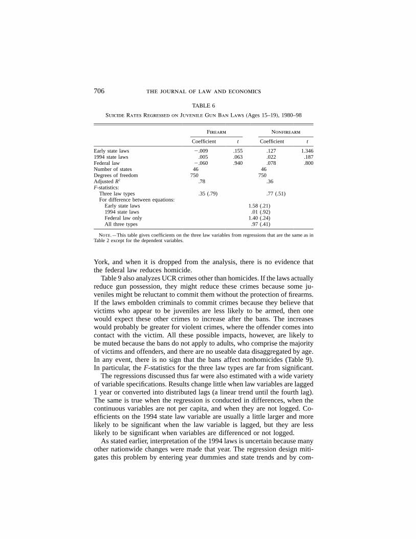
Table 6 gives the results of the analysis of suicides of persons ages 15–19years, presenting only the results concerning the law variables. In regressionssimilar to those in Table 2, the law dummies are never significant and thereis no evidence of a difference between gun and nongun suicide. It is likely,however, that any impact of the laws is dampened in Table 6 because thesuicide measure includes persons 18 and 19 years old, who are not coveredby the gun possession ban, and unlike with the gun homicide measures, onewould expect an exact correspondence between age and impact of the law.

Next, in Tables 7–9, the basic homicide regressions are replicated withseven additional homicide measures, again using dummies for the three typesof laws. Only the law coefficients are shown. The results are consistent withthe gun homicide regressions in Tables 2–4; the 1994 state laws have positivecoefficients, while the federal law has negative coefficients, significant intwo regressions. Coefficients on the federal law are greatly affected by New

24 There is no uniformly accepted way to calculate the standard error of means of coefficients.The procedure used in Table 6 is that recommended in M. Hashem Persaran & Ron Smith,Estimating Long-Run Relationships from Dynamic Heterogenous Panels, 68 J. Econometrics79 (1995). Another procedure is to calculate the standard deviation of the mean by dividingthe mean standard deviation by the square root of the number of law dummies involved (seeBadi H. Baltagi & James M. Griffin, Pooled Estimators vs. Their Heterogeneous Counterpartsin the Context of Dynamic Demand for Gasoline, 77 J. Econometrics 303 (1997)), whichusually produces largert-ratios. Baltagi & Griffin,supra, and Pesaran & Smith,supra, addresscoefficient heterogeneity by conducting separate regressions for each unit. That is not feasiblehere because the time series are too short and, more importantly, because separate regressionsare likely to be misspecified because they lack year effects.

25 One reason for the slight differences between the means in Table 5 and the law coefficientsin Tables 2–4 is that the latter are based on regressions weighted by population, whereas themeans in Table 5 treat each coefficient equally and thus emphasize smaller states. Thus,excluding New York has little impact on the mean for the federal law only states in Table 5.


TABLE 6

Suicide Rates Regressed on Juvenile Gun Ban Laws (Ages 15–19), 1980–98

Firearm Nonfirearm


Early state laws �.009 .155 .127 1.3461994 state laws .005 .063 .022 .187Federal law �.060 .940 .078 .800Number of states 46 46Degrees of freedom 750 750AdjustedR2 .78 .36F-statistics:

Three law types .35 (.79) .77 (.51)For difference between equations:

Early state laws 1.58 (.21)1994 state laws .01 (.92)Federal law only 1.40 (.24)All three types .97 (.41)

Note.—This table gives coefficients on the three law variables from regressions that are the same as inTable 2 except for the dependent variables.

York, and when it is dropped from the analysis, there is no evidence thatthe federal law reduces homicide.

Table 9 also analyzes UCR crimes other than homicides. If the laws actuallyreduce gun possession, they might reduce these crimes because some ju-veniles might be reluctant to commit them without the protection of firearms.If the laws embolden criminals to commit crimes because they believe thatvictims who appear to be juveniles are less likely to be armed, then onewould expect these other crimes to increase after the bans. The increaseswould probably be greater for violent crimes, where the offender comes intocontact with the victim. All these possible impacts, however, are likely tobe muted because the bans do not apply to adults, who comprise the majorityof victims and offenders, and there are no useable data disaggregated by age.In any event, there is no sign that the bans affect nonhomicides (Table 9).In particular, theF-statistics for the three law types are far from significant.

The regressions discussed thus far were also estimated with a wide varietyof variable specifications. Results change little when law variables are lagged1 year or converted into distributed lags (a linear trend until the fourth lag).The same is true when the regression is conducted in differences, when thecontinuous variables are not per capita, and when they are not logged. Co-efficients on the 1994 state law variable are usually a little larger and morelikely to be significant when the law variable is lagged, but they are lesslikely to be significant when variables are differenced or not logged.

As stated earlier, interpretation of the 1994 laws is uncertain because manyother nationwide changes were made that year. The regression design miti-gates this problem by entering year dummies and state trends and by com-


TABLE 7

Homicide Victimization Rates Regressed on Juvenile Gun Ban Laws

1980–98 1977–99

Ages 15–19 Ages 15–24 Ages 14–17 Ages 14–24

Coefficient t Coefficient t Coefficient t Coefficient t

Early state laws �.021 .332 .024 .547 .000 .005 .035 .8791994 state laws .160 1.910 .132 2.285 .157 1.339 .092 1.320Federal law �.063 .932 �.064 1.383 �.166 2.261 �.125 2.817F for three types 2.21 (.09) 3.59 (.01) 3.00 (.03) 4.51 (.004)Number of states 44 49 34 42Degrees of freedom 716 801 672 838AdjustedR2 .87 .92 .80 .89


paring coefficients in gun and nongun homicides. Still, the best estimatesare probably for the pre-1994 laws, which were passed before the spate offederal law activity. There is virtually no evidence that the pre-1994 lawshave an impact.

Another way to control for at least some of the other changes occurringaround 1994 is to add dummy variables for specific laws. I added threecategories to the regressions in Tables 2–4. The first is background checksfor handgun purchases, which under the Brady Act were first applied afterFebruary 1994 in 33 states that did not already have background checks(indicated in Table 1).26 The second is that 24 states have three-strikes laws(usually enhanced penalties for third violent felonies).27 The third is that 25states have shall-issue laws (which facilitate concealed handgun permits).28

These additions had very little impact on the results reported above.29

26 Jens Ludwig & Philip J. Cook, Homicide and Suicide Rates Associated with Implemen-tation of the Brady Handgun Violence Prevention Act, 284 JAMA 585 (2000).

27 See Marvell & Moody,supra note 23.28 See Lott & Mustard,supra note 10. The dates for these laws are as follows: Alaska,

August 30, 1994; Arizona, July 17, 1994; Arkansas, July 8, 1995; Florida, October 1, 1987;Georgia, August 25, 1989; Idaho, July 1, 1990; Kentucky, October 1, 1996; Louisiana, April19, 1996; Maine, August 7, 1980; Mississippi, July 1, 1990; Montana, October 1, 1991; Nevada,October 1, 1995; New Hampshire, August 1, 1994; North Carolina, December 1, 1995;Oklahoma, September 1, 1995; Oregon, January 1, 1990; Pennsylvania, June 18, 1989, andOctober 19, 1995; South Carolina, August 23, 1996; Tennessee, July 1, 1994; Texas, August28, 1995; Utah, May 1, 1995; Virginia, July 1, 1983, and July 1, 1995; West Virginia, July1, 1988; Wyoming, October 1, 1994.

29 Analysis of the results for these three law variables is outside the scope of this paper. Arough summary is that the shall-issue laws have little discernable impact except for reducingrape. The three-strikes laws are strongly associated with increases in almost all measures ofhomicide (the major exceptions are nongun homicides of persons ages 15–19 and 15–24). Thelikely reasons for this result are discussed in Marvell & Moody,supra note 23. The BradyAct is also strongly associated with more homicides (except victimizations of persons ages15–19 and 15–24), as well as with robbery, burglary, and auto thefts. A possible reason isthat criminals believe that citizens are more vulnerable. However, this finding suffers from the


TABLE 8

Homicide Arrest Rates Regressed on Juvenile Gun Ban Laws, 1977–99

Ages 14–17 Ages 14–24


Early state laws .054 .796 .080 1.8431994 state laws .218 1.784 .159 2.103Federal law �.095 1.254 �.070 1.454F for three types 2.31 (.08) 4.03 (.01)Number of states 35 44Degrees of freedom 693 880AdjustedR2 .83 .86


The next analysis is another comparison of coefficients, with young personand adult victimizations as dependent variables. If the juvenile handgun bansact to increase homicides because criminals have less cause to fear thatvictims are armed, then the impact should fall only on persons whom theattacker believes to be juveniles (it is possible, however, that offenders mightrefrain from attacking adults if there are juveniles present whom the offenderbelieves might be armed). Although the bans apply to persons under 18, theattacker often does not know the victim’s age and might believe older personsare similarly without gun protection. In any event, I use victimizations ofpersons ages 14–17, 15–19, and 15–24. Likewise, it is difficult to determinewhich age group is not affected, and the variables used are persons olderthan 19 and persons older than 24. These various combinations lead to fivecomparisons, and there is no indication of a difference between the age groupsfor any of the three law types.

It is possible that the apparent lack of crime-reduction impact of the lawis due to simultaneity—that is, state legislatures pass juvenile bans in responseto rising juvenile homicide, such that this positive relationship counteractsa negative impact of the laws. This possibility is suggested by Figure 1 andTable 1. Most laws in the “early state law” category were enacted in the late1980s and early 1990s, just when juvenile gun homicide was increasing.Although these crimes peaked in about 1992, the 1994 federal and state lawsmight be in response to the trends in the prior decade. This issue is addressedin two ways. First, any such simultaneity would be mitigated (but not elim-inated) by lagging the law dummy variables, because the legislatures are not

fact that the categorization of states as Brady Act states and non–Brady Act states by Ludwig& Cook, supra note 26, has little to do with the extent of gun control exercised before andafter the Brady Act. Several Brady Act states (subjected to the law) already had strong guncontrol laws, while the federal government classified several states as non–Brady Act stateson the basis of laws passed just before the Brady Act went into effect. In all, because of thisproblem and because of the positive coefficients on the Brady Act variable, I question theresults in Ludwig & Cook,supra note 26.

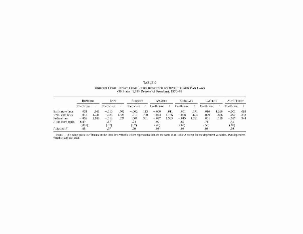
TABLE 9

Uniform Crime Report Crime Rates Regressed on Juvenile Gun Ban Laws(50 States, 1,353 Degrees of Freedom), 1970–99

Homicide Rape Robbery Assault Burglary Larceny Auto Theft

Coefficient t Coefficient t Coefficient t Coefficient t Coefficient t Coefficient t Coefficient t

Early state laws .003 .161 �.010 .702 �.002 .113 �.000 .011 .001 .171 .010 1.260 �.001 .0931994 state laws .051 1.741 �.026 1.326 .019 .790 �.024 1.186 �.008 .604 .009 .856 .007 .333Federal law �.076 3.180 �.013 .827 .007 .361 �.027 1.563 �.015 1.281 .001 .119 �.017 .944F for three types 6.89

(.001).67

(.57).24

(.87).99

(.40).62

(.60).71

(.55).51

(.67)AdjustedR2 .95 .97 .99 .98 .98 .98 .98

Note.—This table gives coefficients on the three law variables from regressions that are the same as in Table 2 except for the dependent variables. Two dependent-variable lags are used.


influenced by crime rates in the next year. As discussed earlier, lagging thedummy has little impact on the results.

Another way to explore possible simultaneity is the Granger test.30 Usinga probit procedure, with the variables listed in Table 2 plus the state effects,the law dummies are regressed on crime lagged 2 years, as well as the lawdummies lagged 2 years. If rising crime caused the laws to be enacted, thecoefficients on the crime variables would be significant and positive.31 Theanalysis showed that there is no evidence of this for any of the three lawcategories and for any of the numerous crime measures. Most coefficientson lagged crime (the regressions use lags of 1 and 2 years) are negative, andnone is positive and significant.

VI. Conclusion

Juvenile handgun bans have little or no impact on a wide variety of crimemeasures. This finding renders the analysis more difficult than if an impactwere found. Most published evaluations of laws do find an impact one wayor another, and they typically only present a regression with significant results,with perhaps a few supporting analyses. Such a procedure, however, is notvalid to show the absence of an impact because still other specificationsmight uncover an apparent impact. Also, the lack of significant results doesnot mean absence of impact, just that it is less likely. One can never claimto have covered all possibilities, but this paper attempts to mitigate these byusing numerous crime measures as well as several configurations of the lawvariables and of the continuous variables. The multiple time-series designusing coefficient comparisons, moreover, provides far more controls thanother procedures.

One can posit theories that the juvenile gun bans either increase or decreasehomicides. If the bans reduce juvenile gun access, they would probably reducethe use of guns by juveniles in crimes. If the bans lead others to believe thatjuveniles are more vulnerable targets, the result is likely to be more crime,especially violent crimes involving juveniles. The finding that the laws havelittle or no impact could mean that both types of theories are without meritor that they cancel each other out. The former appears more likely. It is notlikely that theories cancel each other in a similar way for so many different

30 Clive W. J. Granger, Investigating Causal Relations by Econometric Models and Cross-Spectral Methods, 37 Econometrica 424 (1969).

31 The rationale for the Granger test is that there is no simultaneity between the dependentvariable and lagged independent variable, so long as the lagged dependent variable is enteredto control for possible serial correlation between the lagged independent variable and dependentvariable through the lagged dependent variable. It is possible for the Granger test to misscausation if it occurs only in the current year, since the current year independent variable isnot entered (because the causal direction in the current year is undetermined). This is veryunlikely here because the legislature in one year is unlikely to react only to crime in that yearand not consider crime in the prior year.


crime measures, and the lack of impact on juvenile suicide rates suggeststhat the laws do not reduce gun access.

The results are almost uniform with respect to the pre-1994 state lawsbanning juvenile gun possession: they have no discernible crime-reductionimpact, and there is only very slight evidence of an increase, mainly withrespect to total gun homicides (Table 5). The results for the 1994 law variablesare more uncertain because the results might be influenced by substantialfederal efforts commenced that year to regulate guns and reduce crime gen-erally. Where the 1994 laws seem to have an impact, the suggestion is almostalways that crime increases; thus, there is no evidence that these bans hadtheir intended effect. There is some slight support for the theory that thebans increase homicides because juveniles appear more vulnerable. Withaggregate law variables, this effect appears mainly for state 1994 laws andit is usually counterbalanced by negative results for the federal 1994 law.The strongest indication occurs when the law variable is disaggregated, butthese results are affected by large positive coefficients in a few small states.Finally, there is no discernable difference between the impact of the lawson murders by juveniles and those by adults; if the laws encouraged crime,the impact would only apply to the former.

Bibliography

Allen, Terry, and Buckner, Glen. “A Graphical Approach to AnalyzingRelationships between Offenders and Victims UsingSupplementaryHomicide Reports.” Homicide Studies 1 (1997): 129–40.

Baltagi, Badi H., and Griffin, James M. “Pooled Estimators vs. TheirHeterogeneous Counterparts in the Context of Dynamic Demand forGasoline.”Journal of Econometrics 77 (1997): 303–27.

Blumstein, Alfred, and Cork, Daniel. “Linking Gun Availability to YouthGun Violence.”Law and Contemporary Problems 59 (1996): 5–24.

Bureau of Alcohol, Tobacco and Firearms.Firearms State Laws andPublished Ordinances, 20th ed. Washington, D.C.: Department of theTreasury, 1994.

Cook, Philip J., and Leitzel, James A. “ ‘Perversity, Futility, Jeopardy’: AnEconomic Analysis of the Attack on Gun Control.”Law and ContemporaryProblems 59 (1996): 1–118.

DeFrancesco, Susan. “Children and Guns.”Pace Law Review 29 (1999):275–92.

Donohue, John J., III, and Levitt, Steven D. “Legalized Abortion and Crime.”Quarterly Journal of Economics 116 (2001): 379–420.

Fox, James Alan, and Zawitz, Marianne W.Homicide Trends in the UnitedStates. Washington, D.C.: U.S. Department of Justice, 2000.

Gladwell, Malcolm.The Tipping Point: How Little Things Can Make a BigDifference. Boston: Little, Brown & Company, 2000.


Granger, Clive W. J. “Investigating Causal Relations by Econometric Modelsand Cross-Spectral Methods.”Econometrica 37 (1969): 424–38.

Greene, William H.Econometric Analysis. 2d ed. New York: MacmillanPublishing Co., 1993.

Holden, Gwen A., et al.Compilation of State Firearm Codes that AffectJuveniles. Washington, D.C.: National Criminal Justice Association, 1994.

Lott, John R., Jr., and Mustard, David B. “Crime, Deterrence, and Right-to-Carry Concealed Handguns.”Journal of Legal Studies 26 (1997): 1–68.

Ludwig, Jens. “Concealed-Gun-Carrying Laws and Violent Crime: Evidencefrom State Panel Data.”International Review of Law and Economics 18(1998): 239–54.

Ludwig, Jens, and Cook, Philip J. “Homicide and Suicide Rates Associatedwith Implementation of the Brady Handgun Violence Prevention Act.”JAMA 284 (2000): 585–91.

Maltz, Michael D. “Visualizing Homicide: A Research Note.”Journal ofQuantitative Criminology 14 (1998): 397–410.

Marvell, Thomas B., and Moody, Carlisle E. “Age Structure and Crime Rates:The Conflicting Evidence.”Journal of Quantitative Criminology 7 (1991):237–73.

Marvell, Thomas B., and Moody, Carlisle E. “Determinate Sentencing andAbolishing Parole: The Long-Term Impacts on Prisons and Crime.”Criminology 34 (1996): 107–28.

Marvell, Thomas B., and Moody, Carlisle E. “The Impact of Out-of-StatePrison Population on State Homicide Rates: Displacement and Free-RiderEffects.” Criminology 36 (1998): 513–36.

Marvell, Thomas B., and Moody, Carlisle E. “Female and Male HomicideVictimization Rates: Comparing Trends and Regressors.”Criminology 37(1999): 879–902.

Marvell, Thomas B., and Moody, Carlisle E. “The Lethal Effects of Three-Strikes Laws.”Journal of Legal Studies 30 (2001): 89–106.

National Center for Health Statistics.Vital Statistics of the United States1978. Washington, D.C.: Government Printing Office, 1982.

Pesaran, M. Hashem, and Smith, Ron. “Estimating Long-Run Relationshipsfrom Dynamic Heterogenous Panels.”Journal of Econometrics 68 (1995):79–113.

Rosenberg, Steven. “Just Another Kid with a Gun?United States v. MichaelR.: Reviewing the Youth Handgun Safety Act under theUnited States v.Lopez Commerce Clause Analysis.”Golden Gate University Law Review28 (1998): 51–88.

SAS Institute.SAS/ETS User’s Guide. Version 6, 2d ed. Cary, N.C.: SASInstitute, 1993.

Snyder, Howard N. “The Overrepresentation of Juvenile Crime Proportions


in Robbery Clearance Statistics.”Journal of Quantitative Criminology 15(1999): 151–62.

Wooldridge, Jeffrey M. Introductory Economics: A Modern Approach.Cincinnati: South-Western College Publishing, 2000.

the impact of banning juvenile gun possession

Documents