The Relationship Between Childhood Family Income,

Educational Attainment and Adult Outcomes

Jonathan Eng

Northwestern University

MMSS Senior Thesis 2012

Advisor: Diane Whitmore Schanzenbach

  2  

TABLE OF CONTENTS

Acknowledgements 3

Abstract 4

I. Introduction 5

II. Background and Literature Review 6

III. Data and Methodology 9

IV. Results 15

V. Heterogeneity 28

VI. Oaxaca Decomposition 30

VII. Conclusion 33

Appendices 38

Works Cited 40

  3  

ACKNOWLEDGEMENTS

First, I would like to thank my senior thesis advisor, Professor Diane Whitmore

Schanzenbach, for all of her contributions. Her guidance, time, effort and patience through the

year, even throughout her pregnancy, have made this paper possible. I would also like to thank

the MMSS teaching assistant, Aanchal Jain, for her help with some of the statistical analysis

involved in the research. Finally, I would like to thank my family and friends, who have always

been supportive during my time here at Northwestern.

  4  

ABSTRACT

Historically, evidence has shown that in the United States, less privileged children are at

a disadvantage when it comes to how far they get in school and how much they earn as adults. In

this paper, I examine whether there has been any improvement along this front in past decades,

and whether income inequality and educational inequality are related in any way. Using

longitudinal data from the NELS88, I test for correlation between family income in eighth grade

and educational attainment and employment outcomes twelve years later. I find that family

income remains an important positive predictor of eventual adult outcomes. The effects persist

even when many characteristics that are related to income, such as parents’ education, home

environment characteristics, parental involvement, school characteristics and student ability, are

controlled in a regression framework.

  5  

I. INTRODUCTION

Dr. Martin Luther King Jr. (1967) wrote, “The job of the school is to teach so well that

family background is no longer an issue.” Americans demand much from education, as it has the

potential to create opportunity for anyone, no matter his or her race, gender, or socioeconomic

status. While policies such as No Child Left Behind aim to achieve this goal, equal opportunity

remains a concern for politicians and policy makers alike. Because education has the ability to

raise one’s skill or ability, and there is an economic return to higher skill (Neal and Johnson,

1996), education on a large scale can affect the extent to which intergenerational mobility occurs,

namely whether and how socioeconomic status is passed on from parent to child. In the United

States, we have one of the higher Gini coefficients in the world, as well as a higher score of

inequality of opportunity, two measures which are closely linked (Krueger, 2012). How can we

call America the land of opportunity when the rich and the poor are so far apart, yet remain that

way through generations?

One test for equity in our education system is whether student achievement and

educational attainment is independent of parents’ socioeconomic status. If skill acquisition were

unrelated to family background, in a competitive market, this would likely imply that

employment outcomes would be independent of family SES, which in turn implies more

mobility between classes. On the other hand, if the data demonstrate a significant correlation

between the family income and future income, of which education is a major determinant, this

should raise concerns regarding the education system’s role in the perpetuation of income

inequality in the United States.

  6  

II. BACKGROUND AND LITERATURE REVIEW

Past research has established that low-income students are at a disadvantage in terms of

educational attainment. According to the NLSY97 survey, of children who grew up in families

with income below 130 percent of the poverty line, only 5.6 percent attained a bachelor’s or

higher degree by their last collected interview, while among children who grew up in households

with income greater than 250 percent of the poverty line, 27 percent had completed a bachelor’s

or higher (Barrow and Schanzenbach, 2011). This is consistent with prior research done by Lang

and Ruud (1986) that demonstrated that people from a background of lower socioeconomic

status tend to progress through school more slowly than the general population. Lang and Ruud

further claimed that this tends to be the primary source of the educational achievement gap

stemming from socioeconomic differences.

Conditional on educational attainment, children also have different test scores as it relates

to family socioeconomic status. According to Rouse and Barrow (2006), four years after eighth

grade, those in the highest SES quartile averaged a standardized test score around the 65th

percentile while those in the lowest SES quartile averaged only around the 35th percentile.

Evidence suggests that in the wage market, those with lower observed ability will earn less than

those with higher ability (Neal and Johnson, 1996). This can cause major concern for those who

hope to solve the problem of income inequality; if less advantaged students predictably end up as

lower ability students, and eventually lower-earning adults, we cannot be a fair society while this

disparity continues.

However, while low-income students are at a disadvantage in terms of educational

attainment, does that mean that income inequality is possibly being perpetuated by the education

  7  

system? To show this is much more difficult. It is plausible that despite the fact lower income

students attain less education, there is no significant relationship between parental income and

the income of the child conditional on education. Some may argue lower income students

innately have less ability than higher income students, and therefore they earn less income in the

future in a labor market where ability is rewarded.

Research suggests that this relationship is not entirely driven by innate ability differences.

According to Rouse and Barrow (2006), less privileged students attain less education than high-

income children for several reasons. First, there may be greater psychological costs. Less

advantaged parents tend to have lower educational expectations for their children, and this can

cause the children to have lower confidence in their ability. Secondly, there is the cost of forgone

income from continuing in school instead of getting a job, which is also greater for lower income

families. Lastly, they may experience a lack of access to credit markets, and therefore higher

borrowing costs when it comes to taking out college loans.

Unfortunately, the most recent research shows that the problem may very well be

worsening with time. According to Reardon (2011), the income-related achievement gap is now

almost twice as large as the black-white gap. When comparing children from a family at the 90th

percentile of income distribution with children from a family at the 10th percentile, the

achievement gap has grown from 30 percent for children born in 1976 to 40 percent for those

born in 2001.

By analyzing historical patterns in income inequality, Reardon (2011) concludes that

while rising income inequality may play a role in this growing achievement gap, “it does not

appear to be the dominant factor.” A number of factors could be at work, such as parental

involvement or educational policy focusing on standardized test scores. He concludes to say that

  8  

all of these interconnected factors could possibly be in play, and more research is necessary to

further understand these trends in order to prevent a possible decrease in intergenerational

mobility.

In this paper, I update the existing literature on the relationship between socioeconomic

status and adult outcomes with current data. Throughout the years, educational policy makers

have tried to provide children with more equal inputs in public education in an attempt to close

the gap. Therefore, we might expect the education system to be better today than it was in the

past. However, academic research such as Reardon’s indicates that there may be much work left

to be done. I will explore the evidence and shed light on whether the data suggests any progress

has been made towards a more economically equal society.

  9  

III. DATA AND METHODOLOGY

The National Education Longitudinal Study of 1988 (NELS88) followed over 20,000

eighth graders from 1988 to 2000, which was, for many, four years removed from college

graduation. This survey has a large amount of information on students as well as their parents

and schools. I focus on base-year demographics from the 1988 survey data and the follow-up

data from 2000, the last year of the survey.

A number of variables were considered for the analysis. The base-year demographics

included family size and income, parents’ highest levels of education, school composition, and

math and reading grades and test scores measured in eighth grade. I also considered two

additional vectors of controls, the first of which gauges the amount of resources available at

home, including books, newspapers, magazines, a computer, etc. The other vector measures

parental involvement in school-related activities, which describes both the level of discussion of

school matters with parent(s), as well as parent(s)’ attendance at events such as parent-teacher

conferences, classes and school activities. In the 2000 survey, I focus on income earned in 1999

and the attainment of a high school diploma and four-year post-secondary education degree.

Because this is a longitudinal study, by looking at the relationships between variables in

the base year and in the follow up, I can determine whether family income during childhood has

a predictive role in eventual completed education and adult earnings, after controlling for a

variety of confounding characteristics. In other words, not only do children differ in terms of

their level of family income, but they also differ in terms of a variety of other ways, such as

parental education, home environment, and so on. It is likely that most, if not all, of these factors

influence long-term outcomes. For example, a child with low-income parents who encourage

  10  

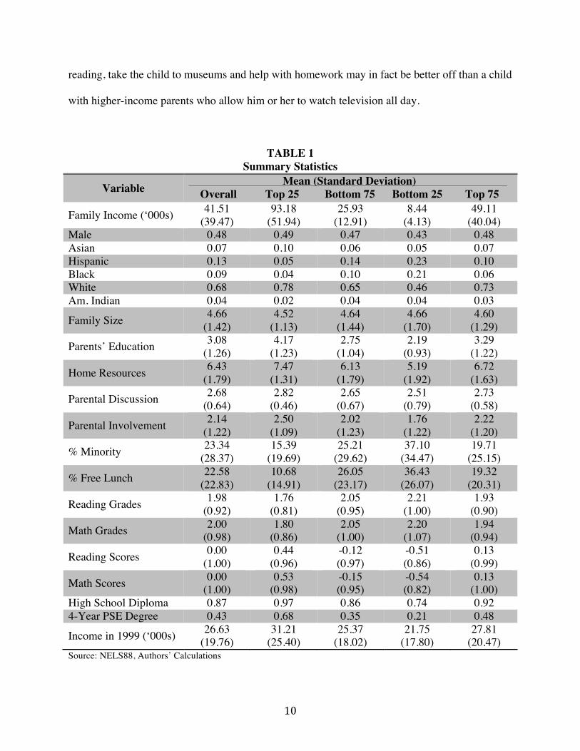
reading, take the child to museums and help with homework may in fact be better off than a child

with higher-income parents who allow him or her to watch television all day.

TABLE 1 Summary Statistics

Variable Mean (Standard Deviation) . Overall Top 25 Bottom 75 Bottom 25 Top 75

Family Income (‘000s) 41.51 (39.47)

93.18 (51.94)

25.93 (12.91)

8.44 (4.13)

49.11 (40.04)

Male 0.48 0.49 0.47 0.43 0.48 Asian 0.07 0.10 0.06 0.05 0.07 Hispanic 0.13 0.05 0.14 0.23 0.10 Black 0.09 0.04 0.10 0.21 0.06 White 0.68 0.78 0.65 0.46 0.73 Am. Indian 0.04 0.02 0.04 0.04 0.03

Family Size 4.66 (1.42)

4.52 (1.13)

4.64 (1.44)

4.66 (1.70)

4.60 (1.29)

Parents’ Education 3.08 (1.26)

4.17 (1.23)

2.75 (1.04)

2.19 (0.93)

3.29 (1.22)

Home Resources 6.43 (1.79)

7.47 (1.31)

6.13 (1.79)

5.19 (1.92)

6.72 (1.63)

Parental Discussion 2.68 (0.64)

2.82 (0.46)

2.65 (0.67)

2.51 (0.79)

2.73 (0.58)

Parental Involvement 2.14 (1.22)

2.50 (1.09)

2.02 (1.23)

1.76 (1.22)

2.22 (1.20)

% Minority 23.34 (28.37)

15.39 (19.69)

25.21 (29.62)

37.10 (34.47)

19.71 (25.15)

% Free Lunch 22.58 (22.83)

10.68 (14.91)

26.05 (23.17)

36.43 (26.07)

19.32 (20.31)

Reading Grades 1.98 (0.92)

1.76 (0.81)

2.05 (0.95)

2.21 (1.00)

1.93 (0.90)

Math Grades 2.00 (0.98)

1.80 (0.86)

2.05 (1.00)

2.20 (1.07)

1.94 (0.94)

Reading Scores 0.00 (1.00)

0.44 (0.96)

-0.12 (0.97)

-0.51 (0.86)

0.13 (0.99)

Math Scores 0.00 (1.00)

0.53 (0.98)

-0.15 (0.95)

-0.54 (0.82)

0.13 (1.00)

High School Diploma 0.87 0.97 0.86 0.74 0.92 4-Year PSE Degree 0.43 0.68 0.35 0.21 0.48

Income in 1999 (‘000s) 26.63 (19.76)

31.21 (25.40)

25.37 (18.02)

21.75 (17.80)

27.81 (20.47)

Source: NELS88, Authors’ Calculations

  11  

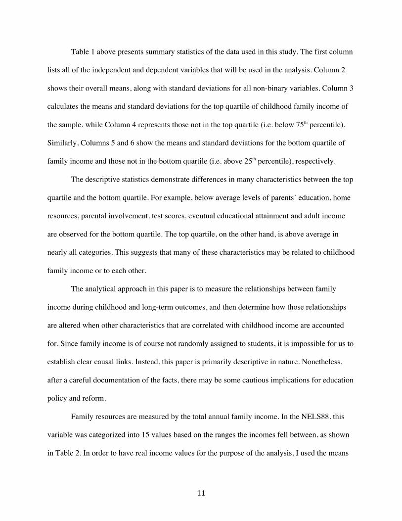
Table 1 above presents summary statistics of the data used in this study. The first column

lists all of the independent and dependent variables that will be used in the analysis. Column 2

shows their overall means, along with standard deviations for all non-binary variables. Column 3

calculates the means and standard deviations for the top quartile of childhood family income of

the sample, while Column 4 represents those not in the top quartile (i.e. below 75th percentile).

Similarly, Columns 5 and 6 show the means and standard deviations for the bottom quartile of

family income and those not in the bottom quartile (i.e. above 25th percentile), respectively.

The descriptive statistics demonstrate differences in many characteristics between the top

quartile and the bottom quartile. For example, below average levels of parents’ education, home

resources, parental involvement, test scores, eventual educational attainment and adult income

are observed for the bottom quartile. The top quartile, on the other hand, is above average in

nearly all categories. This suggests that many of these characteristics may be related to childhood

family income or to each other.

The analytical approach in this paper is to measure the relationships between family

income during childhood and long-term outcomes, and then determine how those relationships

are altered when other characteristics that are correlated with childhood income are accounted

for. Since family income is of course not randomly assigned to students, it is impossible for us to

establish clear causal links. Instead, this paper is primarily descriptive in nature. Nonetheless,

after a careful documentation of the facts, there may be some cautious implications for education

policy and reform.

Family resources are measured by the total annual family income. In the NELS88, this

variable was categorized into 15 values based on the ranges the incomes fell between, as shown

in Table 2. In order to have real income values for the purpose of the analysis, I used the means

  12  

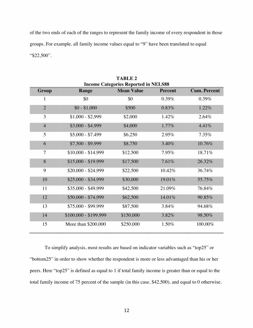
of the two ends of each of the ranges to represent the family income of every respondent in those

groups. For example, all family income values equal to “9” have been translated to equal

“$22,500”.

TABLE 2 Income Categories Reported in NELS88

Group Range Mean Value Percent Cum. Percent 1 $0 $0 0.39% 0.39%

2 $0 - $1,000 $500 0.83% 1.22%

3 $1,000 - $2,999 $2,000 1.42% 2.64%

4 $3,000 - $4,999 $4,000 1.77% 4.41%

5 $5,000 - $7,499 $6,250 2.95% 7.35%

6 $7,500 - $9,999 $8,750 3.40% 10.76%

7 $10,000 - $14,999 $12,500 7.95% 18.71%

8 $15,000 - $19,999 $17,500 7.61% 26.32%

9 $20,000 - $24,999 $22,500 10.42% 36.74%

10 $25,000 - $34,999 $30,000 19.01% 55.75%

11 $35,000 - $49,999 $42,500 21.09% 76.84%

12 $50,000 - $74,999 $62,500 14.01% 90.85%

13 $75,000 - $99,999 $87,500 3.84% 94.68%

14 $100,000 - $199,999 $150,000 3.82% 98.50%

15 More than $200,000 $250,000 1.50% 100.00%

To simplify analysis, most results are based on indicator variables such as “top25” or

“bottom25” in order to show whether the respondent is more or less advantaged than his or her

peers. Here “top25” is defined as equal to 1 if total family income is greater than or equal to the

total family income of 75 percent of the sample (in this case, $42,500), and equal to 0 otherwise.

  13  

The “bottom25” variable has a value of 1 if total family income is less than or equal to the total

family income of 25 percent of the sample ($17,500) and 0 otherwise.

The analysis will mainly look at the relationships between base-year family income and

both the eventual educational attainment (measured twelve years after the baseline survey) and

the income in 1999 of the respondent. The other variables are in our analysis for control

purposes, and thus I will focus on the interpretation of the main coefficient on the measure of

family resources and how this coefficient varies as additional background controls are included.

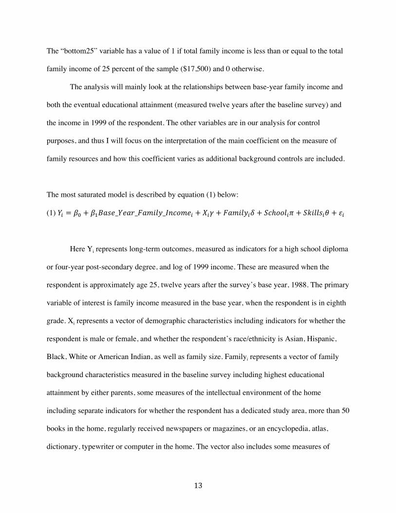
The most saturated model is described by equation (1) below:

(1) 𝑌! = 𝛽! + 𝛽!𝐵𝑎𝑠𝑒_𝑌𝑒𝑎𝑟_𝐹𝑎𝑚𝑖𝑙𝑦_𝐼𝑛𝑐𝑜𝑚𝑒! + 𝑋!𝛾 + 𝐹𝑎𝑚𝑖𝑙𝑦!𝛿 + 𝑆𝑐ℎ𝑜𝑜𝑙!𝜋 + 𝑆𝑘𝑖𝑙𝑙𝑠!𝜃 + 𝜀!

Here Yi represents long-term outcomes, measured as indicators for a high school diploma

or four-year post-secondary degree, and log of 1999 income. These are measured when the

respondent is approximately age 25, twelve years after the survey’s base year, 1988. The primary

variable of interest is family income measured in the base year, when the respondent is in eighth

grade. Xi represents a vector of demographic characteristics including indicators for whether the

respondent is male or female, and whether the respondent’s race/ethnicity is Asian, Hispanic,

Black, White or American Indian, as well as family size. Familyi represents a vector of family

background characteristics measured in the baseline survey including highest educational

attainment by either parents, some measures of the intellectual environment of the home

including separate indicators for whether the respondent has a dedicated study area, more than 50

books in the home, regularly received newspapers or magazines, or an encyclopedia, atlas,

dictionary, typewriter or computer in the home. The vector also includes some measures of

  14  

parental practices, including whether the respondent discusses school with his or her parents,

whether the parents attend school meetings, speak with teachers, visit class, or attend an extra-

curricular event. Schooli is a vector of school-level characteristics measured at baseline including

percentage of minority students and percentage of students receiving free or reduced-price lunch.

Skillsi includes math and reading grades in eighth grade as well as normalized eighth grade

standardized test scores in math and reading. Epsilon represents a mean-zero error term. I

estimate the equation using an ordinary least squares regression.

  15  

IV. RESULTS

Base-year Family Income and Educational Attainment

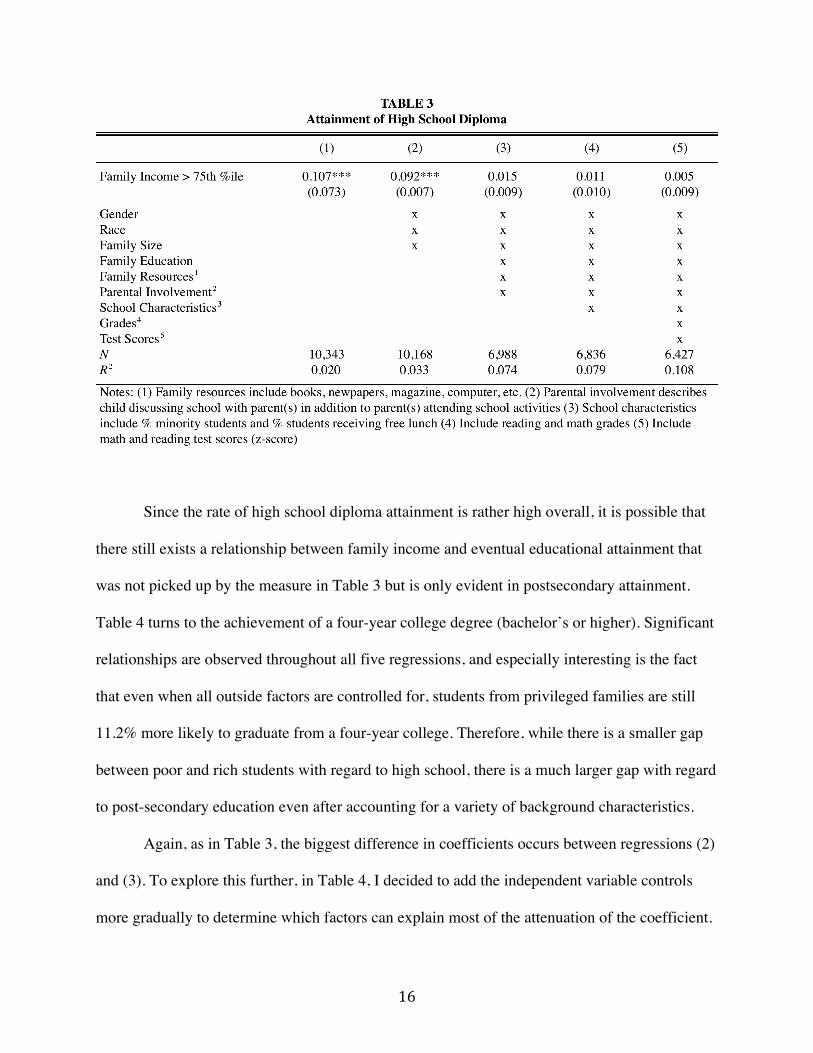
The first set of results tests whether there is correlation between family income and the

achievement of a high school diploma. For students with family income below the 75th

percentile, the baseline rate for high school completion is 86.2%. Table 3 shows that when no

additional factors are controlled, students with families above the 75th percentile in income are

10.7% more likely to complete high school. Column (2) adds controls for gender, race and

family size, but these do little to change the relationship between family income and the

attainment of a high school diploma. As more factors are included, the magnitude and

significance of the relationship declines. The jump from regression (2) to (3) suggests that once

parents’ education, family resources and parental involvement are taken into account, family

income no longer has any additional predictive power for whether a student graduates from high

school. Column (4) includes school characteristics, and column (5) includes the student’s grades

and standardized test scores in the eighth grade. These further attenuate the relationship between

family income and HS diploma attainment, yielding a precisely estimated zero. Note that a

relationship as small as 2.3% can be ruled out at the 5% significance level.

  16  

Since the rate of high school diploma attainment is rather high overall, it is possible that

there still exists a relationship between family income and eventual educational attainment that

was not picked up by the measure in Table 3 but is only evident in postsecondary attainment.

Table 4 turns to the achievement of a four-year college degree (bachelor’s or higher). Significant

relationships are observed throughout all five regressions, and especially interesting is the fact

that even when all outside factors are controlled for, students from privileged families are still

11.2% more likely to graduate from a four-year college. Therefore, while there is a smaller gap

between poor and rich students with regard to high school, there is a much larger gap with regard

to post-secondary education even after accounting for a variety of background characteristics.

Again, as in Table 3, the biggest difference in coefficients occurs between regressions (2)

and (3). To explore this further, in Table 4, I decided to add the independent variable controls

more gradually to determine which factors can explain most of the attenuation of the coefficient.

  17  

Column (2’) adds only family education (i.e. mother’s and father’s highest grade completed,

equal to the highest non-missing value for both parents) and (2’’) adds family resources in the

home (i.e. a specific place for study, books, daily newspaper, regularly received magazines, an

encyclopedia, an atlas, a dictionary, a typewriter and a computer) on top of that. The data suggest

that parents’ education is perhaps the most influential factor in terms of attenuating the

relationship between educational outcomes and family income, cutting the raw coefficient by

nearly half. The addition of all of the remaining variables in Columns (4) and (5) further

attenuates this relationship by another 16 percent.

 

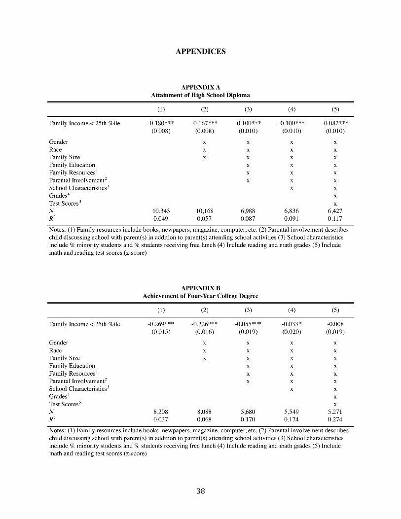
I am also interested in how educational attainment varies when considering the bottom of

the income distribution. In Appendices A and B, I replicate Tables 3 and 4, but this time the

independent variable of interest is an indicator variable for family income lower than the 25th

percentile. The results display different patterns than those observed for the top of the income

distribution, as the predictive power of family background at the bottom of the income

distribution on eventual educational attainment is stronger when considering the high school

  18  

diploma than the four-year college degree. This suggests that low-income students with

otherwise the same characteristics as high-income students are much less likely to graduate from

high school (in fact, 8.2% less), but the ones who do make it past high school are not much

worse off once they reach the collegiate level.

Base-year Family Income and Adult Income

Next, I test the relationship between family income and one’s adult income (measured in

1999, when respondents were approximately 25 or 26 years old). As Table 5 shows, the raw

correlation shows that respondents from families with incomes greater than or equal to the 75th

percentile earn on average to 18.3% more income in 1999. Again, Column (3) includes controls

for parents’ education, resources available at home and parental involvement, while Column (4)

includes school characteristics. Including these variables reduces the relationship between family

income and adult earnings somewhat, but the relationship remains strong, positive and

statistically significant. When the model is saturated to include individual attributes such as

grades and test scores as in Column (5), more privileged children continue to earn 4.9% more, all

else equal. In other words, a rich child with the same exact background characteristics otherwise

would still earn roughly 5% more than a non-rich child. This relationship is statistically

significant at the 10% level.

  19  

Because the relationship between childhood income and adult income may differ across

the distribution, I look to see whether children at the bottom of the income distribution also have

a persistent relationship between family income and adult outcomes. As shown in Table 6, the

raw income difference is 27.3%. Unlike in earlier tables, in which the uncontrolled relationship

is narrowed substantially by the inclusion of other background factors, here we see that the

relationship does not decrease by much as the model is saturated. Even with all controls factored

in, students from poorer families earn 18.2% less than their counterparts. This suggests that there

may be some important nonlinearities in the relationship between family income and adult

outcomes.

  20  

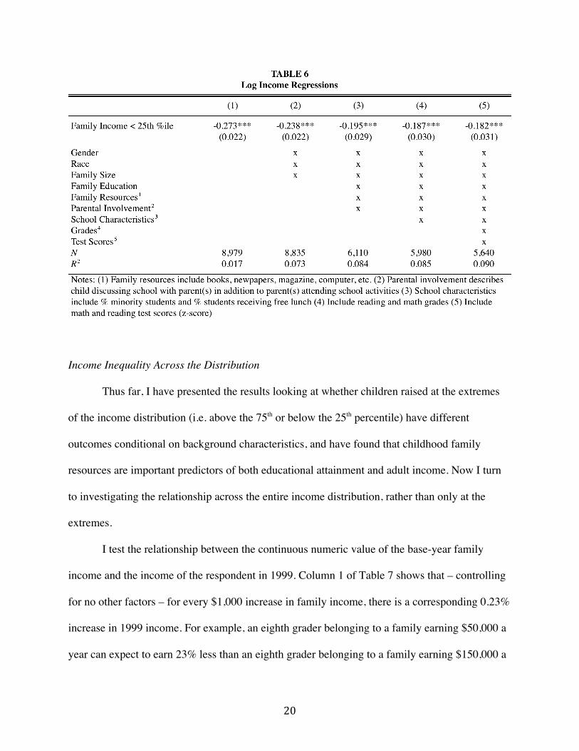
Income Inequality Across the Distribution

Thus far, I have presented the results looking at whether children raised at the extremes

of the income distribution (i.e. above the 75th or below the 25th percentile) have different

outcomes conditional on background characteristics, and have found that childhood family

resources are important predictors of both educational attainment and adult income. Now I turn

to investigating the relationship across the entire income distribution, rather than only at the

extremes.

I test the relationship between the continuous numeric value of the base-year family

income and the income of the respondent in 1999. Column 1 of Table 7 shows that – controlling

for no other factors – for every $1,000 increase in family income, there is a corresponding 0.23%

increase in 1999 income. For example, an eighth grader belonging to a family earning $50,000 a

year can expect to earn 23% less than an eighth grader belonging to a family earning $150,000 a

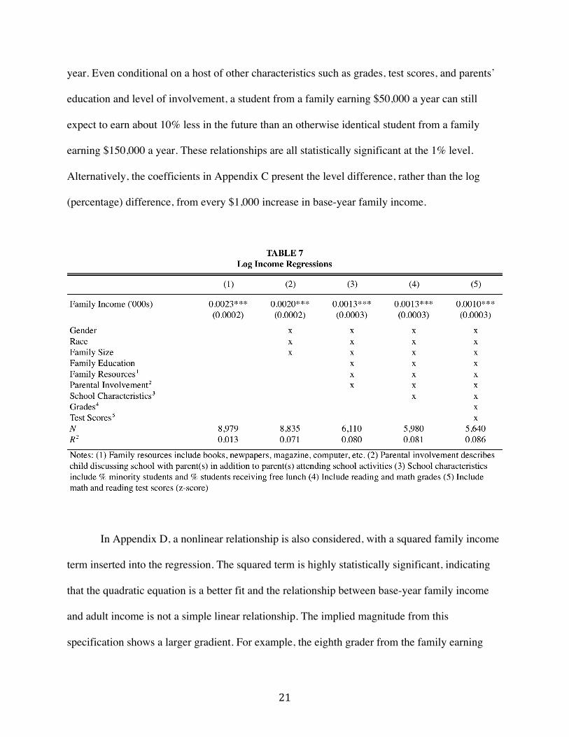
  21  

year. Even conditional on a host of other characteristics such as grades, test scores, and parents’

education and level of involvement, a student from a family earning $50,000 a year can still

expect to earn about 10% less in the future than an otherwise identical student from a family

earning $150,000 a year. These relationships are all statistically significant at the 1% level.

Alternatively, the coefficients in Appendix C present the level difference, rather than the log

(percentage) difference, from every $1,000 increase in base-year family income.

In Appendix D, a nonlinear relationship is also considered, with a squared family income

term inserted into the regression. The squared term is highly statistically significant, indicating

that the quadratic equation is a better fit and the relationship between base-year family income

and adult income is not a simple linear relationship. The implied magnitude from this

specification shows a larger gradient. For example, the eighth grader from the family earning

  22  

$50,000 a year can now expect to earn 44% less than the eighth grader from the family making

$150,000 a year – almost twice the magnitude estimated from the linear specification – when no

other controls are included. With all other characteristics controlled for, the implied income gap

in this example is 25%, compared to 10% in the parallel linear specification.

Non-parametric Relationship Between Family Income and Adult Outcomes

Next, I look throughout the distribution at the relationship between childhood family

income and the outcomes of interest, namely post-secondary education degree attainment and

adult income. The following charts show the regression results when family income is dummied

out into 15 categories as originally done by the NELS88 survey (described in the Data section).

Each chart shows the mean income on the x-axis and the coefficient on the y-axis. The annual

family income ranges and means are presented in Table 2.

Chart 1 below shows the relationship between attainment of a four-year post-secondary

education degree and the family income group, with no other characteristics controlled for in the

model. The solid purple line represents the estimated betas for the corresponding incomes, while

the dotted purple lines represent the upper and lower bounds of the confidence intervals. Relative

to the lowest income group, Group 1, there is no statistically significant difference in the

likelihood of four-year post-secondary education completion for those growing up in any income

group through Group 11. The point estimates are negative through Group 9, but again, not

statistically significantly different from zero. Relative to the lowest income group, those in

Group 12 are 28.6% more likely to obtain a four-year college degree. Children from even higher

income families (Groups 13-15) have a statistically significant 43 to 55 percent advantage in

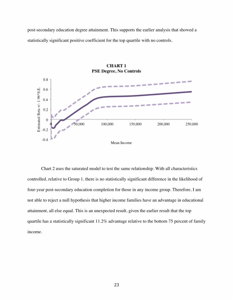
  23  

post-secondary education degree attainment. This supports the earlier analysis that showed a

statistically significant positive coefficient for the top quartile with no controls.

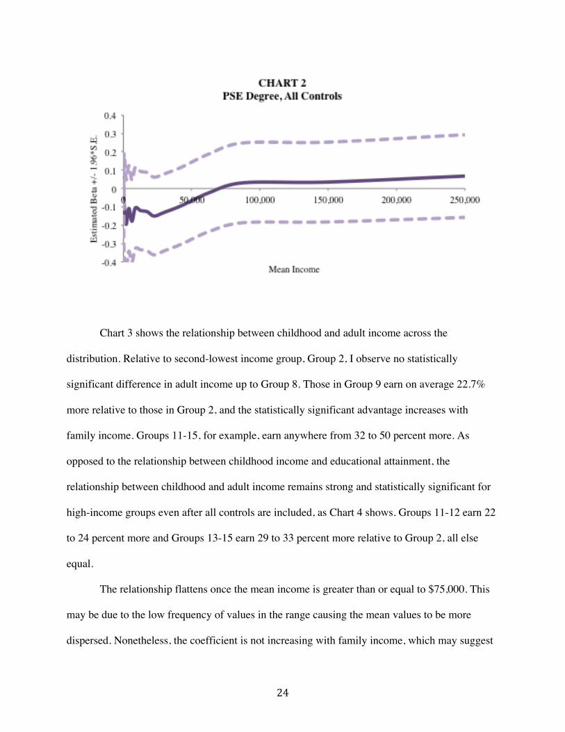
Chart 2 uses the saturated model to test the same relationship. With all characteristics

controlled, relative to Group 1, there is no statistically significant difference in the likelihood of

four-year post-secondary education completion for those in any income group. Therefore, I am

not able to reject a null hypothesis that higher income families have an advantage in educational

attainment, all else equal. This is an unexpected result, given the earlier result that the top

quartile has a statistically significant 11.2% advantage relative to the bottom 75 percent of family

income.

  24  

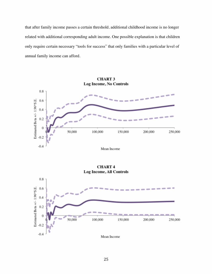
Chart 3 shows the relationship between childhood and adult income across the

distribution. Relative to second-lowest income group, Group 2, I observe no statistically

significant difference in adult income up to Group 8. Those in Group 9 earn on average 22.7%

more relative to those in Group 2, and the statistically significant advantage increases with

family income. Groups 11-15, for example, earn anywhere from 32 to 50 percent more. As

opposed to the relationship between childhood income and educational attainment, the

relationship between childhood and adult income remains strong and statistically significant for

high-income groups even after all controls are included, as Chart 4 shows. Groups 11-12 earn 22

to 24 percent more and Groups 13-15 earn 29 to 33 percent more relative to Group 2, all else

equal.

The relationship flattens once the mean income is greater than or equal to $75,000. This

may be due to the low frequency of values in the range causing the mean values to be more

dispersed. Nonetheless, the coefficient is not increasing with family income, which may suggest

  25  

that after family income passes a certain threshold, additional childhood income is no longer

related with additional corresponding adult income. One possible explanation is that children

only require certain necessary “tools for success” that only families with a particular level of

annual family income can afford.

  26  

Income Inequality and Education

So far, the evidence from my analysis shows that income inequality is correlated to both

educational attainment as well as employment outcomes through earned income. Originally

proposed in the Introduction, an important question that remains is how much of the variation in

adult income is explained by differences in educational attainment. To test for this, I add direct

controls for educational attainment into the model predicting adult income. Note that if the

relationship between childhood and adult income is zero once education is controlled for, this

implies that all of the differences in outcomes are driven by differences in education attainment.

On the other hand, if controlling for educational attainment does little to attenuate the

relationship, then this implies that there are other factors not reflected in differential education

outcomes that are driving the relationship.

The model including the additional control for educational attainment is described by equation

(2) below:

(2)

𝑌! = 𝛽! + 𝛽!𝐵𝑎𝑠𝑒_𝑌𝑒𝑎𝑟_𝐹𝑎𝑚𝑖𝑙𝑦_𝐼𝑛𝑐𝑜𝑚𝑒! +  𝛽!𝐻𝑖𝑔ℎ_𝑆𝑐ℎ𝑜𝑜𝑙_𝐷𝑖𝑝𝑙𝑜𝑚𝑎! +  𝛽!𝑃𝑆𝐸_𝐷𝑒𝑔𝑟𝑒𝑒!  

+ 𝑋!𝛾 + 𝐹𝑎𝑚𝑖𝑙𝑦!𝛿 + 𝑆𝑐ℎ𝑜𝑜𝑙!𝜋 + 𝑆𝑘𝑖𝑙𝑙𝑠!𝜃 + 𝜀!

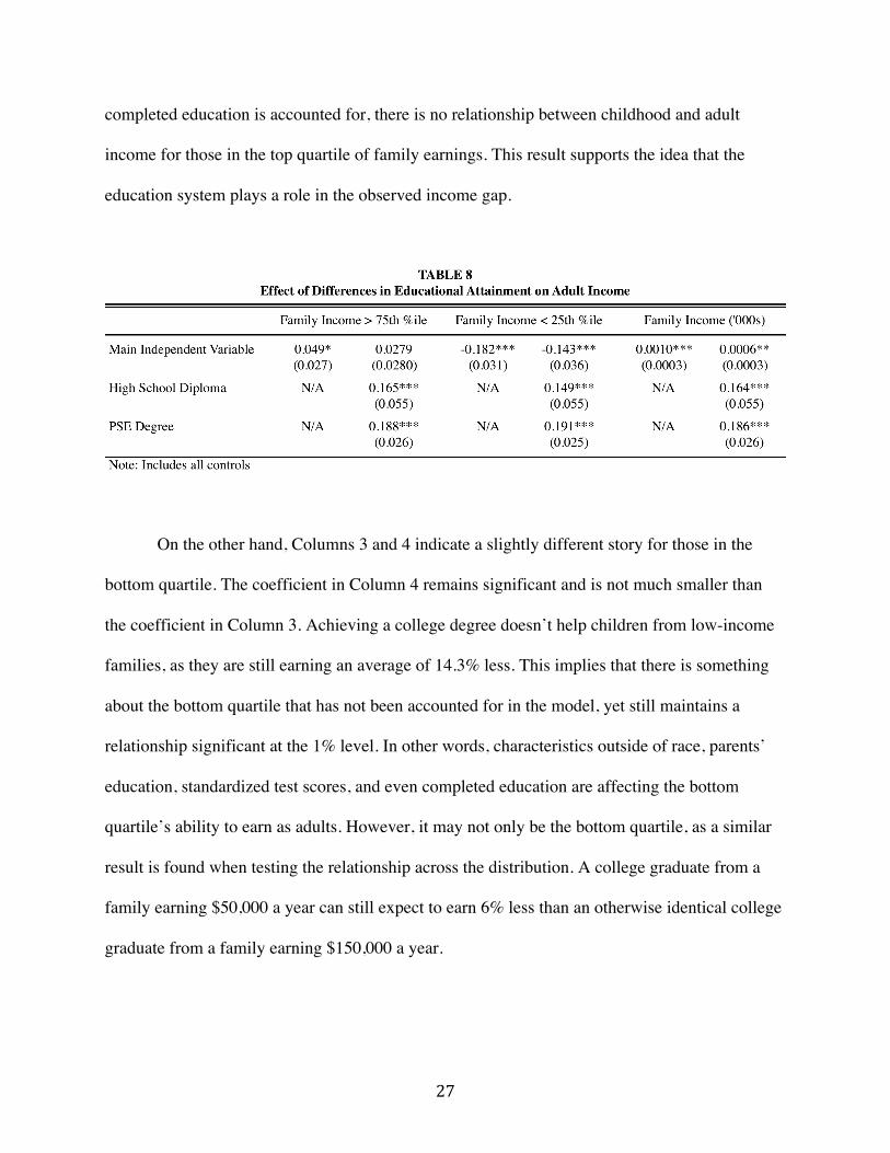
Table 8 shows the change in the coefficients for the three different regressions (i.e. with

“top25”, “bottom25” and family income as the independent variables of interest). For each pair

of columns, the first column is without educational attainment controlled for, while the second

column is with educational attainment controlled for. Columns 1 and 2 suggest that once

  27  

completed education is accounted for, there is no relationship between childhood and adult

income for those in the top quartile of family earnings. This result supports the idea that the

education system plays a role in the observed income gap.

 

On the other hand, Columns 3 and 4 indicate a slightly different story for those in the

bottom quartile. The coefficient in Column 4 remains significant and is not much smaller than

the coefficient in Column 3. Achieving a college degree doesn’t help children from low-income

families, as they are still earning an average of 14.3% less. This implies that there is something

about the bottom quartile that has not been accounted for in the model, yet still maintains a

relationship significant at the 1% level. In other words, characteristics outside of race, parents’

education, standardized test scores, and even completed education are affecting the bottom

quartile’s ability to earn as adults. However, it may not only be the bottom quartile, as a similar

result is found when testing the relationship across the distribution. A college graduate from a

family earning $50,000 a year can still expect to earn 6% less than an otherwise identical college

graduate from a family earning $150,000 a year.

  28  

V. HETEROGENEITY

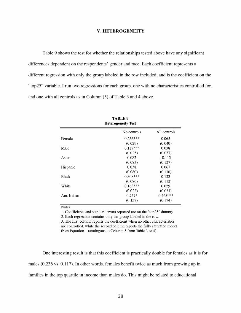
Table 9 shows the test for whether the relationships tested above have any significant

differences dependent on the respondents’ gender and race. Each coefficient represents a

different regression with only the group labeled in the row included, and is the coefficient on the

“top25” variable. I run two regressions for each group, one with no characteristics controlled for,

and one with all controls as in Column (5) of Table 3 and 4 above.

One interesting result is that this coefficient is practically double for females as it is for

males (0.236 vs. 0.117). In other words, females benefit twice as much from growing up in

families in the top quartile in income than males do. This might be related to educational

  29  

expectations, which may be why the significance of the relationship goes away once factors such

as parents’ education and test scores are accounted for.

Regarding race, black students gain the most from more advantaged backgrounds, as

shown by the high coefficient (0.308), versus the lower coefficient for white students (0.163).

Again, the magnitude of these coefficients as well as the statistical significance of the

relationships is attenuated as the model is saturated. In contrast, Asian and Hispanic students

seem to benefit very little, if at all, from family income.

  30  

VI. OAXACA DECOMPOSITION

One alternative methodology to study group differences in adult outcomes is called the

Blinder-Oaxaca decomposition. For my analysis, I will use it to divide the adult income

differential observed between high- and low-income children. There are two methods for the

decomposition: the threefold decomposition, which breaks down the wage gap into the

endowments, coefficients and interaction parts, and the twofold decomposition, which breaks it

down into a part that is “explained” by group differences in background characteristics, and a

part that is “unexplained” (Jann, 2008).

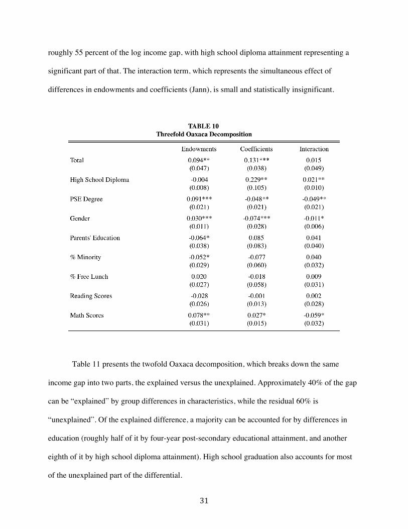
The threefold Oaxaca decomposition, shown in Table 10, divides the log income gap

observed between the bottom quartile and the rest of the sample. Though I included all controls

from the saturated model in Equation 2 in the analysis, Table 10 only presents selected variables

that are either statistically significant or interesting in another way. The prediction for those

above the 25th percentile is 3.145, while the prediction for the bottom quartile is 2.904, resulting

in a difference of 0.240, which is statistically significant at the 1% level. This can be interpreted

as a 24.0% wage gap between the bottom quartile and everyone else.

The differential is then broken down into three separate parts. The endowments term

represents the mean increase in income that those in the bottom quartile would earn if they had

the same characteristics as those who were not in the bottom quartile. In this sample, the increase

of 0.094 in the sample indicates that differences in characteristics in the model account for 39

percent of the entire gap, most of which is due to differences in higher education and math test

scores. The coefficients term quantifies the change in the bottom quartile’s wages when applying

the top 75 percentile’s coefficients to the bottom quartile’s characteristics. This accounts for

  31  

roughly 55 percent of the log income gap, with high school diploma attainment representing a

significant part of that. The interaction term, which represents the simultaneous effect of

differences in endowments and coefficients (Jann), is small and statistically insignificant.

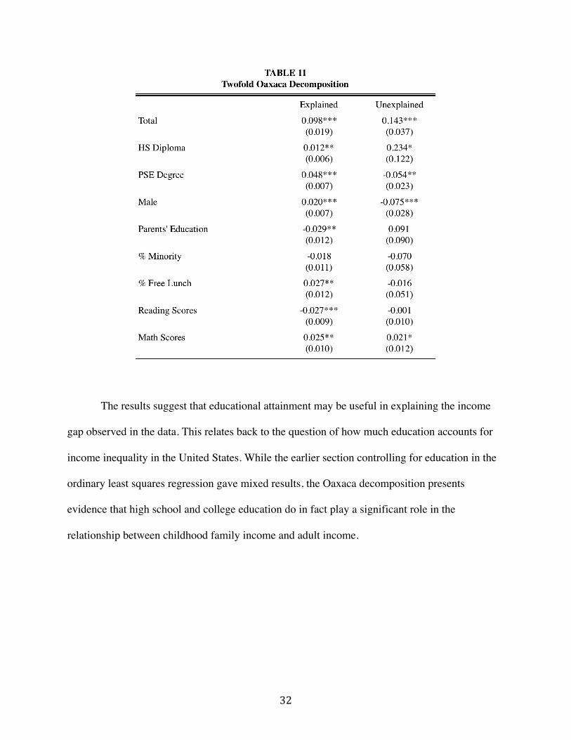
Table 11 presents the twofold Oaxaca decomposition, which breaks down the same

income gap into two parts, the explained versus the unexplained. Approximately 40% of the gap

can be “explained” by group differences in characteristics, while the residual 60% is

“unexplained”. Of the explained difference, a majority can be accounted for by differences in

education (roughly half of it by four-year post-secondary educational attainment, and another

eighth of it by high school diploma attainment). High school graduation also accounts for most

of the unexplained part of the differential.

  32  

The results suggest that educational attainment may be useful in explaining the income

gap observed in the data. This relates back to the question of how much education accounts for

income inequality in the United States. While the earlier section controlling for education in the

ordinary least squares regression gave mixed results, the Oaxaca decomposition presents

evidence that high school and college education do in fact play a significant role in the

relationship between childhood family income and adult income.

  33  

VII. CONCLUSIONS

In the analysis of the NELS88, we discovered some correlation between base-year

demographics and educational attainment. While family income and high school diploma

achievement are not significantly related when an indicator for whether total annual family

income is in the top quartile is used, the relationship is significant when an indicator for whether

family income is in the bottom quartile is used. In other words, in terms of finishing high school,

it doesn’t matter much whether the eighth grader is high-income or not, just as long as he or she

is not low-income.

With regard to attaining a degree from a four-year college, the result is somewhat of the

opposite. There is a strong, significant relationship between family income and achievement of

college degree, with parents’ education perhaps the biggest factor, when the 75th percentile

indicator is used. However, the relationship is insignificant in the saturated model when the 25th

percentile indicator is used. This suggests that being high-income is an advantage to completing

college, but being low-income isn’t necessarily a disadvantage. One possible explanation is that

those who have already made it past high school fare just as well as their peers do once they

arrive at college.

Unsurprisingly, those from more well off families earn more in adulthood. In fact, one

interesting result is that even with all controls, including parents’ education, family resources,

parental involvement, school characteristics and student ability, held constant, those from more

well off families still earn 5% more than their peers. Students from families in the bottom

quartile earn 18.2% less than their peers with all controls factored in. Incrementally, each $1,000

increase in base year family income is correlated to a 0.23% increase in adult annual income, i.e.

  34  

a $100,000 difference in family income can expect to become a 23% difference in future

earnings with no controls, and a 0.10% increase, i.e. $100,000 difference leads to a 10%

difference, with all controls. Additionally, the relationship between base-year family income and

adult income may not be linear. Nonlinearity with a squared term in the equation would mean

that a $100,000 difference in childhood income leads to a 25% difference with all controls held

constant. This indicates that there may even be less intergenerational mobility than previously

suggested.

In the non-parametric analysis, while the control characteristics attenuate the relationship

between family income and four-year college completion, the relationship between family

income and adult income persists after the controls are included. Relative to the second lowest-

income group, those who grew up in families with more than $75,000 in annual income earn

about 30% more as adults. This provides further evidence for income inequality that cannot be

fixed by parenting techniques or even success in middle school.

To test whether educational attainment can explain the income differential, completed

education controls are included in the equation. Once completed education is accounted for, this

zeroes the relationship between base-year family income and adult income for students in the top

quartile of family earnings. However, for the bottom quartile, the relationship exists even when

educational attainment is controlled for. Therefore, there are characteristics outside of the

controls used in the analysis that explain the relationship, but have not been identified. Similarly,

controlling for completed education does not meaningfully affect the correlation between

childhood and adult income, which remains statistically significant at the 5% level.

A Blinder-Oaxaca decomposition exploring the same question yields slightly different

results. In the threefold Oaxaca decomposition, differences in higher education and high school

  35  

education explain a significant part of the log income gap. In the twofold decomposition, of the

“explained” part of the differential, post-secondary education accounts for about 50 percent and

high school education accounts for about 12 percent. This may seem to contradict the earlier

findings, but there is a possible explanation. When adding the educational attainment controls to

the regression, there remained unobserved, unidentifiable factors causing the gap. What the

Oaxaca decomposition tells us, in part, is that for the portion of the gap that we can explain,

education explains much of it.

Limitations & Implications for Further Research

Several limitations on our data prevent our results from being conclusive. The first issue

with the NELS88 is that in a longitudinal study, the timeframe during which the data is collected

is somewhat arbitrary. The specific years of the base-year survey, 1988, and the selected follow-

up study, 2000, are randomly selected. For example, there may be factors (e.g. the dotcom

bubble) that cause the year 1999 to be a worse year for certain portions of the population versus

others. In other words, the relationship may look different for a different 8th grade cohort.

Also, a respondent’s income when he or she is 25 or 26 years old (approximately 3-4

years after graduation of a four-year postsecondary institution) may not be most representative of

adult income. Perhaps adults’ incomes at 35 or 40 years ago are better assessments of their true

earning power. Similarly, the eighth grade might not be the most appropriate time to measure all

of the base-year characteristics. It can be argued that the most essential period of a child’s

development lies within the child’s earlier years. Reardon (2011) suggests that by the time

children enter kindergarten, the income achievement gap he finds is already present. Therefore, it

  36  

might be more optimal to control for home resources and parental practices at age 5 instead of at

age 13, but such data are not currently available.

Another limitation with the data came with the presentation of the family income

variable. As described in the Data section, instead of using continuous values, the NELS report

the income data in 15 categories. While the data were useful for my analysis, it may have been

even more useful to have the continuous numerical values of each family’s annual income. For

example, using the number $250,000 as the representative value for the highest-earning group

(more than $200,000 per year) was somewhat arbitrary.

Aside from confirming the results outlined in this paper, further research should focus on

looking for the additional quantifiable factors that can explain more of the poor-rich gap, because

even with all of the controls in the saturated model, there are undoubtedly omitted variables that

may chip away at some more of the relationships if that data was available. The more research

done to pinpoint some of these factors, the better institutions such as government, charter

schools, and nonprofits can work to counteract them and aim towards providing an equal playing

field for all children regardless of background.

Educational and Social Policy Implications

The next question is: where do we go from here? Using this analysis and future research

in the upcoming years, hopefully a blueprint can be drawn up to address some of these

outstanding issues. The results imply that the education system does play a significant part in the

income inequality in the United States today. Therefore, to close the income gap, we must strive

for more equity in education.

  37  

College admissions may not be as effective as they should be in admitting the right

students. Ideally, the admissions should reflect student ability, but high-income students are

graduating at a higher rate conditional on math and reading grades and test scores. Perhaps it is a

matter of choice for lower-income students, but the financial ability to attend and graduate from

a four-year institution must factor into the decision. Some suggestions may be to examine how

public higher education can be restructured to specifically fit the needs of low-income students,

or to make serving low-income students a priority over seeking prestige in lists such as the US

News and Report rankings.

Another possible explanation for education as a determinant in the relationship between

growing up in the top quartile and earning more as an adult, all else equal, is the exposure of

high-income students to higher quality education, whether in high school or post-secondary

institutions. If that is the case, then the goal would be to increase the quality of the schools that

less privileged children have access to. This may include more public funding of urban schools,

more social services to counteract unstable home environments, increasing teacher and principal

quality and effectiveness, and changing the curriculum to better suit less privileged students.

  38  

APPENDICES

  39  

  40  

WORKS CITED

Barrow, Lisa and Cecilia Elena Rouse. 2006. U.S. Elementary and Secondary Schools:

Equalizing Opportunity or Replicating the Status Quo? The Future of Children 16 (Fall): 99-

123.

Barrow, Lisa and Diane Whitmore Schanzenbach. "Education and the Poor" Oxford Handbook

of the Economics of Poverty. Ed. Philip N. Jefferson. Oxford: Oxford University Press, 2012.

Jann, Ben. 2008. The Blinder-Oaxaca Decomposition for Linear Regression Models. The Stata

Journal 8 (Q4): 453-479.

Johnson, William R., and Derek A. Neal. 1996. The Role of Premarket Factors in Black-White

Wage Differences. Journal of Political Economy 104 (October): 869-895.

King, Martin Luther. Where Do We Go from Here: Chaos or Community? New York: Harper &

Row, 1967.

Krueger, Alan. “The Rise and Consequences of Inequality.” PowerPoint presentation for the

Center for American Progress (CAP). 2012.

Lang, Kevin and Paul A. Ruud. 1986. Returns to Schooling, Implicit Discount Rates and Black-

White Wage Differentials. The Review of Economics and Statistics 68 (February): 41-47.

Manove, Michael and Kevin Lang. 2011. Education and Labor Market Discrimination. American

Economic Review 101 (June): 1467-1496.

Reardon, Sean F. (in press). The Widening Socioeconomic Achievement Gap: New Evidence

and Possible Explanations. Social Inequality and Economic Disadvantage. Washington, DC:

Brookings Institution.