This article is (c) Emerald Group Publishing and permission has been

granted for this version to appear here (centaur.reading.ac.uk). Emerald

does not grant permission for this article to be further copied/distributed or

hosted elsewhere without the express permission from Emerald Group

Publishing Limited. The definitive version can be found at

http://www.emeraldinsight.com/journals.htm?articleid=1659741

2

An Extreme Value Theory Approach to Calculating

Minimum Capital Risk Requirements

by

C. Brooks, A. D. Clare and G. Persand1

Abstract

This paper investigates the frequency of extreme events for three LIFFE futures contracts for

the calculation of minimum capital risk requirements (MCRRs). We propose a semi-

parametric approach where the tails are modelled by the Generalized Pareto Distribution and

smaller risks are captured by the empirical distribution function. We compare the capital

requirements form this approach with those calculated from the unconditional density and

from a conditional density - a GARCH(1,1) model. Our primary finding is that both in-sample

and for a hold-out sample, our extreme value approach yields superior results than either of

the other two models which do not explicitly model the tails of the return distribution. Since

the use of these internal models will be permitted under the EC-CAD II, they could be widely

adopted in the near future for determining capital adequacies. Hence, close scrutiny of

competing models is required to avoid a potentially costly misallocation capital resources

while at the same time ensuring the safety of the financial system.

June 2001

Keywords: Minimum Capital Risk Requirements, Generalized Pareto Distribution, GARCH

models.

JEL Classifications: C14, C15, G13

1 We would like to thank Salih Neftci for useful conversations that improved this paper, and an anonymous

referee for constructive comments. The authors are all members of the ISMA Centre, Dept of Economics,

University of Reading, Whiteknights Park, PO Box 242, Reading, RG6 6BA, United Kingdom. Author for

correspondence: Chris Brooks, tel: (+44) 118 931 67 68; fax: (+44) 118 931 47 41; e-mail: C.Brooks@rdg.ac.uk.

1

1. Introduction

From a regulatory perspective, the notion that financial institutions should hold risk-adjusted

capital as a buffer against potential losses was given international credibility2 in the BIS Basle

Accord of 1988 (see Basle Committee on Banking Supervision, 1988), now widely agreed to

be a landmark document in the regulation of financial institutions. While the original Accord

focused upon credit risk, regulators have since worked on the treatment of market risk. The

calculation of a financial institution’s Value at Risk (VaR) is rapidly becoming the

standardized approach to the determination of appropriate levels of bank capital. In the EU

under the Capital Adequacy Directive II3 for example, the use of internal risk management

models (IRMM), of which J.P. Morgan RiskMetricsTM

(1996) is the most widely known, is

now permitted as long as the institutions can demonstrate that the model, and the operational

procedures relating to the model, are “sound”. The IRMMs are used to identify the amount of

capital required for each (netted) securities position to cover all but a small proportion of

potential losses (typically 5.00%). The sum of these positions is the firm’s value at risk

relating to its trading exposures.

The standard value at risk methodology4 assumes that the underlying return generating

distribution for the security in question is normally distributed, with moments which can be

estimated using past data and do not vary over time. The assumption that the underlying

return generating process is normal and stationary over time leads to an under-estimation of

both the number and size of extreme events. It is commonly accepted that asset return

distributions are fat-tailed. Neftci (1998) argues that it is possible and indeed very likely that

extreme events are “structurally” different from the return generating process that operates

2 Although regulators in the USA and in particular the UK had been operating a risk related system of capital

regulation before this date. 3 See Basle Committee on Banking Supervision (1995).

2

during less extreme market conditions. Under such circumstances - where liquidity in markets

dries up and where routine hedging relationships break down, or become more expensive to

execute - the underlying statistical assumption of normality becomes entirely inappropriate.

We can think of three such events in the recent past: the “Asian crisis” in September 1997, the

“Russian debt crisis” of August 1998, and the “Brazilian crisis” of January 1999. While these

crises were not unrelated, each of them was to some degree associated with abnormal trading

conditions. For example, after the Russian debt crisis, it was reported that liquidity in the

corporate bond market had “dried up” against the background of a “flight to quality” where

market participants paid premium prices for US Treasuries and UK gilts.

In this paper we calculate Minimum Capital Risk Requirements (MCRRs) for three of the

London International Financial Futures Exchange’s (LIFFE) most popular derivatives

contracts. We use an unconditional model, a GARCH(1,1) model and a combination of a

Generalized Pareto Distribution and the empirical distribution of the returns. Our main finding

is that both back-tests and out-of-sample tests of the calculated MCRRs show that the

proportion of exceedences produced by the extreme value approach, which concentrates on the

tails, are considerably closer to the nominal probability of violations than competing

approaches which fit a single model for the whole distribution. The rest of this paper is

organized as follows: in Section 2 we present the data sets; in Section 3 we present the

extreme value theory; in Section 4 we consider alternative models of conditional volatility; we

outline our basic methodology for calculating MCRRs in Section 5; in Section 6 we present

our results; and we conclude the paper in Section 7 with suggestions for future research.

4 For a critical appraisal see Danielsson and DeVries (1997), or Neftci 1998.

3

2. Data

In this study we calculate MCRRs for three LIFFE futures contracts - the FTSE-100 Index

Futures Contract, the Long Gilt Futures Contract and the Short Sterling Interest Rate Futures

Contract - based upon their daily settlement prices5. The Long Gilt contract trades a notional

10-15 year gilt with a yield to maturity of 7%. The Short Sterling contract is based on a 3-

month time deposit with a face value of £500,000. Thus the buyer of such a contract is

allocated this amount as a time deposit in an eligible bank on the delivery date, although ut

may instead be cash settled at the option of the buyer. Note therefore that the “Long” and

“Short” terminology used in the contract titles therefore refers to the contract maturities and

not to a long or short position. The data was collected from Datastream International, and

spans the period 24/05/1991 to 16/09/1996. Sample observations corresponding to UK public

holidays (i.e., when LIFFE was closed) were deleted from the data set to avoid the

incorporation of spurious zero returns, leaving 1344 observations, or trading days in the

sample. In the empirical work below, we use the daily log return of the original price series.

It is evident from Table 1 that all three returns series show strong evidence of skewness – the

FTSE-100 and Short Sterling contract returns are skewed to the right while the returns on the

Long Gilt contract are skewed to the left. They are also highly leptokurtic (i.e. fat-tailed). In

particular, the Short Sterling series has a coefficient of excess kurtosis of nearly 200. The

Jarque-Bera test statistic consequently rejects normality for all three derivative return series.

The extreme fat-tailed nature of the three series provides a strong motivation for the

estimation methodologies employed in this paper that focus on the tails.

[insert table 1 here]

5 Because these contracts expire 4 times per year - March, June, September and December - to obtain a

continuous time series we use the closest to maturity contract unless the next closest has greater volume, in which

case we switch to this contract.

4

3. Extreme Value Theory

Assuming that n21 x,,x,x are the realized returns of some data generating process X6

observed on days n,,2,1 , then let nY denote the highest daily returns (the maximum)7 found

below a certain level of x . In practice, the distribution of the “parent variable” )X( is not

accurately known, therefore the exact distribution of the extremes is also unknown. Thus,

most studies focus upon the asymptotic behaviour of the extremes. Extreme value theory is the

study of the limiting distribution of the order statistic nY ,

yFxYP Y

w

nnn [1]

where, n is the location parameter and n (assumed to be positive) is the location

parameter. w stands for weak convergence and yFY is one of the three asymptotic

distributions as defined below. If the above equation holds, then it can be said that the

distribution function of n21 x,,x,x belongs to the domain of attraction of yFY . The three

distributions, given below, have been justified as the limiting stable distributions of extreme

value theory.

The Gumbel distribution (type 1):

y

Y eexpyF for y [2]

The Fréchet distribution (type 2):

0k0yforyexp

0yfor0yF

kY [3]

6 X represents the log price changes.

7 The example given concentrates on the maximum values only. However, an application to minimum values

would follow a comparable derivation.

5

The Weibull distribution (type 3):

0yfor0

0k0yforyexpyF

k

Y [4]

The shape parameter k reflects the weight of the tail in the distribution of the parent variable

X . The lower is k , the fatter is the distribution of X . It also gives the number of finite

moments of the distributions, for example, when k is greater than unity the mean of the

distribution exists, whereas when it is greater than two the variance is finite and so on.

However, k as well as n and n (known as the “normalizing coefficients”) may be different

for minima and maxima (see Longin, (1996)).

The tail of the distribution of XF is either declining exponentially (type 1) or by a power (type

2) or is finite (type 3). According to Gnedenko (1943): the Gumbel distribution can be the

limit of bounded and unbounded distributions; only distributions unbounded (to the right) can

have a Fréchet distribution as the limit; and only distributions with a finite right end point can

have the Weibull distribution as its limit.

The above three distributions can be grouped together by a generalized formula (see

Jenkinson, 1955):

0ifyfor

0ifyfory.1expyF

1

11

Y

[5]

The tail index, , is related to the shape parameter k by k1 . Thus, the tail index

determines the type of distribution. 0 corresponds to a Gumbel distribution whereas 0

6

corresponds to a Fréchet distribution and 0 to a Weibull distribution. However, it should

be noted that for small values of , i.e., large values of k , the Fréchet and Weibull

distributions are very close to the Gumbel distribution.

Other fat-tailed distributions, for example, the Student-t and the Pareto distributions among

others can be linked to the three extreme value distributions above. Gnedenko (1943) has

given necessary and sufficient conditions for a particular distribution to belong to one of the

three distributions whereby these conditions can be employed in specific cases to derive the

type of asymptotic distribution of extremes. As such, the normal distribution can be seen to

lead to the Gumbel distribution; the Student-t obeys the Fréchet distribution with a shape

parameter k equal to its degrees of freedom; the stable Paretian law, introduced by

Mandelbrot (1963), leads to the Fréchet distribution with a shape parameter k equal to its

characteristic exponent.

The distribution adopted in this paper is the generalized Pareto distribution given by the

following equation:

k1

yk11k,;yG

[6]

where, k is arbitrary, with the range of y being y0 if 0k and ky0 if 0k .

This equation is elaborated below and its interpretation as a limiting distribution is similar to

that which motivates equation [5], and thus the idea behind the generalized Pareto distribution

is fairly similar to that of the extreme value distributions, collected together in the generalized

formula of [5]. Thus the generalized Pareto distribution is employed in this paper forr its

intuitive appeal and since it effectively encompasses the three limiting distributions of

extreme value theory as special cases.

7

Let txF denote the unknown distribution function of the incremental changes in the log of

financial futures prices, the asymptotic theory of extremes is used in approximating the tail

areas of txF . This approach follows Pickands (1975), Smith (1987), Davison and Smith

(1990), Embrechts et al. (1997) and Neftci (1998).

Closely following Smith (1987) and Neftci (1998), we derive the Generalized Pareto

Distribution below. Let U and L represent the two thresholds of the tails, with U representing

the ‘Upper’ threshold and L representing the ‘Lower’ one, such that 0Uxt and

0Dxt lie in the two tails of the distribution txF . The example derived below is for

the upper tail only, however, the replication for the lower tail is similar. The following

probability distribution of the random variable tx can be defined as:

UFUxP t [7]

where, 0xU , and 1xxP 0t , i.e., tx is bounded by 0x .

Now assuming that te , with Ret , is the exceedance of the threshold U at time t, then

ttt eUFeUxP [8]

where, Uxe0 0t .

tU eF is given by

UF1

UFeUFeF t

tU

[9]

with tU eF representing the conditional distribution of Uxt given that Uxt .

8

Following Pickands (1975), tU eF can be approximated by the generalized Pareto

distribution k,;eG u

t with

0,0ke1

0,0kke

11k,;eG

ue

u

k1

u

t

u

t

ut

[10]

where k is arbitrary, with the range of te being te0 if 0k and ke0 u

t if

0k . The case of 0k is interpreted as the limit 0k , i.e. the exponential distribution

with mean u .

Pickands showed that the above equation arises as a limiting distribution for excesses over

thresholds if and only if the parent distribution is in the domain of attraction of one of the

extreme value distributions. The motivation for the equation is the ‘threshold stability’

property, i.e., if te is generalized Pareto and 0U , then the conditional distribution of

Uet (given Uet ) is also generalized Pareto. Another property is as follows: if n (the

number of exceedances) has a Poisson distribution and, conditioning on n , n1 e,,e are iid

generalized Pareto random variables, then n1 e,,emax also has a generalized extreme

value distribution (see Davison and Smith, 1990, pp. 395).

Going back to Equations [9] and [10], the distance between k,;eG u

t and tU eF will

converge to zero as 0xU , i.e. the further we go into the tails:

0k,;eGeFsuplim u

ttUxe0xU

0t0

[11]

9

However, further conditions for tU eF must be satisfied for the above equation to hold, see

Pickands (1975) for more details. Moreover, the (.)G is expected to be a ‘good’

approximation of the (.)FU as long as the threshold level is high enough. However, an

important question would be: ‘how high to fix this threshold?’ This topic is elaborated in the

final part of this section.

The parameters to be estimated from the generalized Pareto distribution are u and k .

Methods for estimating the generalized Pareto distribution parameters have been reviewed by

Hosking and Wallis (1987). Whereas maximum likelihood estimators exist in large samples

provided that 1k , they are asymptotically normal and efficient when 21k (Smith,

1985). Using the same approach as Neftci (1998), the parameters u and k are obtained by

maximizing the log likelihood function of k,;eG u

t .

Assuming that U is high enough so that the generalized Pareto distribution k,;eG u

t with

0k is a good approximation for the probability tU eF , then:

k1

u

t

tt

i

i

ke11exP

[12]

The above equation holds for 0k . In the case that 0k , the condition ke u

t must be

satisfied for the density to be well defined.

Following the expression [12], the density function of tx can be approximated at an

arbitrary observation point it

e , by the density teG :

10

1

t

u

k1

u

t

u

u

t keke

k,;eG

[13]

Finally, by using the density of k,;eG u

t at each observation point, it

e , the following log

likelihood function is obtained

n

1iu

t1

u

tuu iike

1lnkke

1lnlnn,k

[14]

where, n is the number of exceedances in a sample of N observations. In this case, the

sample of extremes ( n ) is obtained by first estimating the standard deviation of the whole

sample of the returns and secondly, by selecting all positive and negative increments greater

than 1.645 times the standard deviation of the sample in absolute terms to represent the

extremes ( n ).

The results for the estimation of n , (the normalizing coefficient) and k (the coefficient

determining the fatness of the tail) are given in Table 2(i).

[table 2 here]

The number of extremes ( n ) for the upper tail is higher than those of the lower tail, except for

the Long Gilt contract whereby the number of extremes is 44 in the lower tail compared to 29

in the upper tail. As expected, u is positive for all three contracts, highest for the FTSE-100

index contract, followed by the Long Gilt and then the Short Sterling contracts. The result is

quite similar for the lower tail: L is positive for all the contracts, highest for the FTSE-100

index contract, followed by the Short Sterling and then the Long Gilt contracts. Whereas the

parameter k is positive in the lower tail for all three contracts (the highest being for the Long

11

Gilt contract, followed by the Short Sterling and FTSE-100 Index contracts), it is negative for

the FTSE-100 Index and Long Gilt contracts in the upper tail.

The next step is to estimate the threshold, T , since it is important to know where the tail starts

for the calculation of the MCRRs. Following the definition of U and L,

L,UmaxT [15]

Using the approximation given in expression [9],

i

i

t

teG

UF1

UFeUF

[16]

the following term is obtained by cross-multiplying:

UFeGeGUF1eUF1iii ttt [17]

UF is unknown but since it is the unconditional probability that an observation will exceed

the level U , a possible estimate is obtained by using the sample frequency, i.e.,

N

nUF [18]

Following Neftci (1998), the estimate of the tail probability is

it

eUF1

k1

u

t

ˆ

ek1

N

ni

[19]

where, u and k are the maximum likelihood estimates of u and k respectively. Denoting

this tail probability estimate by :

k1

uˆ

Tk1

N

n

[20]

Thus, rearranging [20] we obtain the threshold:

12

k

n

N1

k

ˆT

[21]

Again the result for T (for both the upper and lower tails) is presented in Table 2(ii), with

is set at 0.01 in this paper. For the upper tail, the threshold (i.e. the start of the tail) is set at

0.017 for the FTSE-100 Index contract, at 0.010 for the Long Gilt contract and at 0.003 for the

Short Sterling contract. Thus, the threshold is further in the tail for the FTSE-100 Index,

followed by the Long Gilt and the Short Sterling contracts. The same result is obtained for the

lower tail, with the threshold being 0.018 for the FTSE-100 Index contract, 0.010 for the Long

Gilt contract and 0.002 for the Short Sterling contract. The threshold is higher in the lower tail

for the FTSE-100 Index contract compared to the upper tail. On the other hand, the threshold

is higher in the upper tail for the Short Sterling contract compared with its lower tail.

4. GARCH modelling

In order to provide a benchmark for the evaluation of the results from the extreme value

estimation we also calculate MCRRs using a GARCH model. The simple GARCH (1,1)

model is given below:

ttx

1t

2

1tt hh [22]

where, x Log P Pt t t ( / )1 , t t th 1 2/ , t N(0,1).

Following Brooks et al., (2000), the “best” model of conditional volatility from a large set of

candidate models was shown to be the GARCH(1,1) model for all three contracts.

13

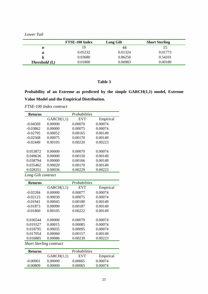
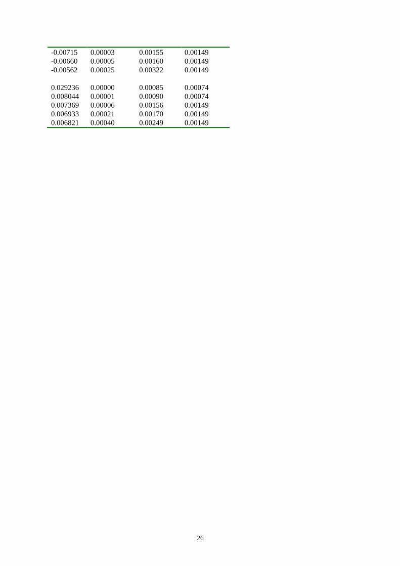
For the purposes of comparison, the probability of an extreme as predicted by the simple

GARCH(1,1) model, Extreme Value model and the empirical distribution is estimated. Table

3 shows the probability of the five highest and lowest returns of the three financial futures

contracts as predicted by the extreme value procedure, the GARCH(1,1) model together with

the values that are predicted by the original empirical distribution function8.

[table 3 here]

For the GARCH(1,1) model, the conditional volatility is predicted and the probability of an

outcome equal to or more extreme than the observed return (conditional on the predicted

volatility for each observation) is recorded. In the case of the extreme value procedure, returns

are estimated by bootstrapping from the Pareto distribution and the interior of the empirical

distribution for common observations. This estimation technique is elaborated in the following

section.

As noted, the probability as predicted by the extreme value procedure, and the values that are

predicted by the empirical distribution are very similar. On the other hand, it can be seen that

the GARCH(1,1) model performs poorly in modelling the tail events compared with the

extreme value approach.

5. A methodology for estimating MCRRs

Capital risk requirements are estimated for 1 day, 1 week, 1 month and 3 month investment

horizons by simulating the conditional densities of price changes, using Efron’s (1982)

bootstrapping methodology. For the Generalized Pareto Distribution model, simulation is

carried out by bootstrapping from both the fitted tails and the empirical distribution function.

8 The distribution function of the log price changes of the contracts.

14

For the GARCH model, since the standardized residuals ( / /t th 1

1 2 ) from these models are iid

(according to the BDS test - see Brooks et al., 2000) the t are drawn randomly, with

replacement, from the standardized residuals and a path of future xt’s can be generated, using

the estimates of , , and from the sample and multi-step ahead forecasts of th .

In the case of the Generalized Pareto Distribution, the path for future prices is simulated as

follows: (1) draw tx from the empirical distribution with replacement, (2) if )L(Txt , then

draw from the generalized Pareto distribution fitted to the lower tail, (3) however, if

)U(Txt , then draw from the generalized Pareto distribution fitted to the upper tail, (4) on

the other hand, if tx falls in the middle of the empirical distribution, i.e. )U(Tx)L(T t ,

then tx is retained. The number of draws of tx is equal to the length of the investment

horizon. This procedure can be considered as a type of structured Monte Carlo study, where

we pay particular attention to the extreme returns in the tails of the distribution. It will be these

extreme returns which most strongly influence the value of the MCRR, and hence most

influence the likelihood of financial distress.

In practice a securities firm undertaking this procedure would have to simulate the price of the

contract when it initially opened the position. To calculate the appropriate capital risk

requirement, it would then have to estimate the maximum loss that the position might

experience over the proposed holding period9. For example, by tracking the daily value of a

long futures position and recording its lowest value over the sample period, the firm can report

its maximum loss per contract for this particular simulated path of futures prices. Repeating

9 The current BIS rules state that the MCRR should be the higher of the (i) average MCRR over the previous 60

days or (ii) the previous trading days’ MCRR. At the time of writing, it is not clear how CAD II will require the

exact calculation to be made.

15

this procedure for 20,000 simulated paths generates an empirical distribution of the maximum

loss. This maximum loss (Q) is given by:

ContractsxxQ )( 10 [23]

where 0x is the price at which the contract is initially bought or sold; and x1 is the lowest

simulated price (for a long position) or the highest simulated price (for a short position) over

the holding period. Assuming (without loss of generality) that the number of contracts held is

1, we can write the following:

0

1

0

1x

x

x

Q [24]

In this case, since 0x is a constant, the distribution of Q will depend on the distribution of 1x .

Hsieh (1993) assumed that prices are lognormally distributed, i.e. that the log of the ratios of

the prices,

0

1

x

xLn , are normally distributed. However, in this paper, we do not impose this

restriction, but instead

0

1

x

xLn

is transformed into a standard normal distribution by

matching the moments of

0

1

x

xLn ’s distribution to one of a set of possible distributions

known as the Johnson (1949) distribution. Matching moments to the family of Johnson

distributions (Normal, Lognormal, Bounded and Unbounded) requires a specification of the

transformation from the

0

1

x

xLn distribution to a distribution that has a standard normal

distribution. In this case, matching moments means finding a distribution, whose first four

moments are known, i.e. one that has the same mean, standard deviation, skewness and

kurtosis as the

0

1

x

xLn distribution.

16

For all the samples of the three contracts, the

0

1

x

xLn distributions were found to match the

Unbounded distribution. Therefore, the estimated 5th

quantile of the

0

1

x

xLn ’s distribution is

based on the following transformation:

cd

b

a

x

xLn

t

645.1sinh

,10

1 [25]

a, b, c and d are parameters whose values are determined by the

0

1

x

xLn ’s first 4 moments.

From expression 7, it can be seen that the distribution of 0x

Q will depend on the distribution of

0

1

x

x. Hence, the first step is to find the 5

th Quantile of

0

1

x

xLn :

Sd

mx

xLn

0

1

[26]

where is the 5th

Quantile from the Johnson Distribution, m is the Mean of

0

1

x

xLn

and

Sd is the Standard Deviation of

0

1

x

xLn . Cross-multiplying and taking the exponential,

mSdlExponentiax

x

0

1 [27]

therefore

mSdlExponentiax

Q 1

0

[28]

17

We also use the unconditional density to calculate MCRRs so that we can make a direct

comparison between this and the two other approaches since this much simpler approach

ignores both the non-linear dependence in the conditional volatility (which would be captured

by the GARCH formulation) and the fat tails of the returns series (which would be accounted

for using the extreme value approach). To use the unconditional density, the xt’s are drawn

randomly, with replacement, from the in-sample returns.

Confidence intervals for the MCRRs are estimated using the jackknife-after-bootstrap

methodology (Efron & Tibshirani, 1993). These confidence intervals are estimated to give an

idea of the likely sampling variation in the MCRR point estimates and help determine whether

the differences in the MCRRs for the conditional and unconditional models are significantly

different.

Assuming that,

%)5(0

1

x

xLn

N(m*,Sd*) then, the confidence interval for the Ln

x

x

1

0 5%)

(

is

%)5(0

1

%)5(0

1

x

xLnSE*960.1

x

xLn

Therefore, the confidence interval of

%)5(0

1

x

x

is

%)5(0

1

%)5(0

1

x

xLnSE*960.1

x

xLnExp

and the confidence interval of

%)5(0x

Q

is given by

%)5(0

1

%)5(0

1

x

xLnSE*960.1

x

xLnExp1

18

The jackknife-after-bootstrap provides a method of estimating the variance of the 5th

quantile

of ln(x1/x0) using only information in the 20,000 bootstrap samples.

To verify the accuracy of this methodology, we compared the actual daily profits and losses of

the three futures contracts with their daily MCRR forecasts. In this case, instead of expression

(6) we will work with the following:

ContractsxxQ tt )( 1 [29]

where tx is the price of the contract at time t and 1tx is the simulated price at time t+1. This

will give us a time series of daily MCRR forecasts. Our measure of model performance is a

count of the number of times the MCRR “underpredicts” realized losses over the sample

period. This procedure is effectively a back-test of the model’s adequacy over the in-sample

estimation period.

However, for a fuller evaluation of the results we need to perform an out-of-sample test of the

MCRRs based upon the three models, to determine whether the models are likely to be useful

in the practical situation where we are determining the capital requirement to cover a period in

the future when the parameters of the models are estimated using past data. We therefore

calculated MCRRs for a 1 day investment horizon for each contract and for both short and

long positions on day t and then checked to see whether this MCRR had been exceeded by

price movements in day t+1. We rolled this process forward, recalculating the MCRRs etc.,

for 500 days, i.e. using the sample period 17th

September 1996 to 12th

August 1998. Out-of-

sample tests are not commonly applied in this literature, but are an essential part of the model

evaluation process, since it is likely that back-tests will over-state the success of all models,

since the data used to assess the adequacy of the MCRR calculations, has also been used to

19

determine the parameters of the models. Moreover, back-tests are likely to be biased towards

profligate models which fit to sample-specific features of the data, but are unable to generalize

in a genuine out-of-sample forecasting environment.

6. The MCRRs

The MCRRs for the three contracts based upon the unconditional density, the GARCH(1,1)

and EVT models are presented in Table 4.

[table 4 here]

Close inspection of the results reveals that the MCRRs are always higher for short compared

with long futures positions, particularly as the investment horizon is increased. This is

because the distribution of log-price changes is not symmetric: there is a larger probability of a

price rise in all three futures contracts than a price fall over the sample period (i.e., the mean

returns in Table 1 are all positive), indicating that there is a greater probability that a loss will

be sustained on a short relative to a long position. For example, the MCRR for a long Short

Sterling position, calculated using the GARCH(1,1) model and held for three months is

3.627%, but is 5.798% for a short position.

The MCRRs based upon the GARCH(1,1) model are always higher than for the unconditional

density method of calculation. This result highlights the excess volatility persistence implied

in the GARCH(1,1) model (see Hsieh, 1993, for a discussion of this issue). A higher degree

of persistence implies that a large innovation in contract returns (of either sign) causes

volatility to remain high for a relatively long period, and therefore the amount of capital

required to cover this protracted period of higher implied volatility is also higher. The effect

of this volatility persistence is considerable – with MCRRs increasing by a factor of two or

20

three in most cases, compared with those generated from the unconditional density. For

example, the MCRR GARCH(1,1) estimate for a Short Sterling contract position is 3.627%

for a three month investment horizon, whereas the comparable figure for the unconditional

density is 1.643%. For the extreme value theory approach, the MCRRs tend to be smaller than

the GARCH(1,1) model but greater than the Unconditional Density for the FTSE-100 Index

and the Short Sterling contracts, however those for the Long Gilt are smaller than both the

conditional and unconditional volatility models. Moreover, capital requirements are highest

for the contract which is most volatile, i.e. the FTSE-100 stock index futures contract, while

the Short Sterling contract is least volatile of the three and therefore requires less of a capital

charge. This holds true for all three alternative methods of estimation.

Approximate 95% confidence intervals for the MCRRs calculated from the unconditional

density, the GARCH model and the EVT approach are presented in Table 5.

[table 5 here]

The most important feature of these results is the “tightness” of the intervals around the

MCRR point estimates. For example, the 95% confidence interval around the MCRR point

estimates of 12.028% for a Long Gilt contract position of three months is 11.787% to

12.509%. Also, in the cases of all three contracts the confidence intervals for the conditional

GARCH and unconditional density models as well as the extreme value theory approach never

overlap. This indicates that there is a highly statistically significant difference between the

MCRRs generated using the conditional GARCH, the EVT and unconditional density.

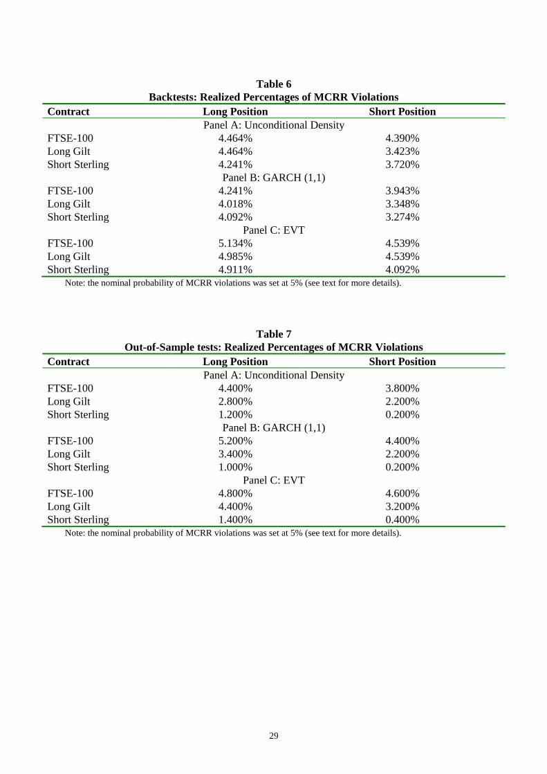
Table 6 presents the proportion of times that the MCRR is violated during the estimation

sample.

[table 6 here]

21

The back-testing results show that the realized percentages of MCRR violations (for both long

and short positions) are in general lower than the nominal 5% coverage. The same holds true

for the other two models. Thus, although all the models give rather different sets of MCRRs,

the out-of-sample tests show that they are all adequate for the estimation of minimum capital

requirements, i.e., the realized percentages of MCRR violations is 5% or less than 5% (with

the exception of the EVT model for a long position in the FTSE contract, which is 5.1%).

However, if the proportion of exceedences is considerably less than 5%, this implies that the

capital charge has been set too high and thus bank capital is tied up in an unnecessary and

unprofitable way. In this regard, the extreme value model yields the best results overall, since

the proportion of exceedences is much closer to the nominal 5% level while for the others the

number of exceedences is too few. In general, the extreme value-generated MCRRs have a

proportion of violations which is up to a percentage point higher than those from the

unconditional and GARCH models. The most noticeable improvement is for a long position in

the Short Sterling contract, where EVT gives 4.9% of exceedences, compared with 4.46 and

4.24 for the unconditional and GARCH models respectively.

The out-of-sample testing results, shown in table 7, are also highly supportive to the extreme

value approach compared with its competitors.

[table 7 here]

For example, considering a long position in the Long Gilt contract, the proportion of

violations is 2.8% for the unconditional density, and 3.4% for the GARCH model, while it is

4.4% for the MCRR generated using extreme value theory. The superior performance of the

extreme value approach indicates that a securities firm who adopted this methodology, could

cut is capital requirement by up to one third while still retaining a number of violations which

is within acceptable limits.

22

6. Conclusions

Under CAD II European banks and investment firms will be able to calculate appropriate

levels of capital for their trading books using IRMMs10. It is expected that these models will

be in widespread usage, particularly in London, soon after the necessary legislation has been

passed. Given this development in the international regulatory environment, in this paper we

investigated certain aspects of this technology by calculating MCRRs for three of the most

popular derivatives contracts currently trading on LIFFE.

Our results demonstrate the usefulness of the extreme value approach in providing a superior

fit to the data and giving improved back-testing and out-of-sample results. Further research in

this area might consider the application of such techniques to other data series or the

consideration of alternative fat-tailed distributions. Since the use of these internal models will

be permitted under the EC-CAD II, they could be widely adopted in the near future for

determining capital adequacies. Hence, close scrutiny of competing models is required to

avoid wastage of capital resources whilst at the same time ensuring the safety of the financial

system.

10

This proposal is due to be adopted by the EU’s Council of Ministers and the European Parliament under the co-

decision procedure.

23

References

Basle Committee on Banking Supervision, 1995, April, An Internal Model-Based Approach to

Market Risk Capital Requirements

Basle Committee on Banking Supervision, 1988, July, International Convergence of Capital

Measurement and Capital Standards

Brooks, C., A.D. Clare and G. Persand, 2000, A Word of Caution on Calculating Market-

based Minimum Capital Risk Requirements, Journal of Banking and Finance 14(10), 1557-

1574

Brock, W., W.Dechert, J.Scheinkman and B. LeBaron, 1996, A Test for Independence based

on the Correlation Dimension, Econometric Reviews 15, pp 197-235.

Clifford Chance, 1998, CADII moves forward, Newsletter: European Financial Markets,

London.

Danielsson, J. and C.G. De Vries, 1997, Value-at-Risk and Extreme Returns, LSE Working

Paper Presented at the Issues of Empirical Finance (Financial Market Group), Nov 1997.

Davison, A.C. and R.L Smith, 1990, Models for Exceedances of High Thresholds, The

Journal of Royal Statistical Society 52(3), pp. 393-442.

Efron, B., 1982, The Jackknife, the Bootstrap, and Other Resampling Plans, Philadelphia, PA:

Society for Industrial and Applied Mathematics.

Efron, B., and R.Tibshirani, 1993, An Introduction to the Bootstrap, Chapman Hall.

Gnedenko, B.V., 1943, Sur la distribution limite du terme maximum d’une série aléatoire,

Annals of Mathematics 44, pp 423-453.

Gumbel, E.J., 1958, Statistics of Extremes. Columbia University Press, New York.

Hsieh, D.A., 1993, Implications of Nonlinear Dynamics for Financial Risk Management,

Journal of Financial and Quantitative Analysis 28, pp 41-64.

Jenkinson, A.F., 1955, The Frequency Distribution of the Annual Maximum (or Minimum)

Values of Meteorological Elements, Quarterly Journal of the Royal Meteorology Society 87,

pp 145-158.

Johnson, N.L., 1949, Systems of Frequency Curves Generated by Methods of Translations,

Biometrika, pp149-175.

J.P. Morgan, 1996, Riskmetrics Technical Document 4th Edition.

Longin, F.M., 1996, The Asymptotic Distribution of Extreme Stock Market Returns, Journal

of Business 69 (3), pp 383-408.

24

Mandelbrot, B., 1963, The Variation of Certain Speculative Prices, Journal of Business 36, pp

394-419.

Neftci, S.N., 1998, Value-at-Risk Calculations, Extreme Events and Tail Estimation, Mimeo,

Graduate School and University Centre of CUNY.

Pickands, 1975, Statistical Inference Using Extreme Order Statistics, Annals of Statistics Vol

3, No1, pp 119-131.

Smith, R.L., 1985, Maximum Likelihood Estimation in a Class of Nonregular Cases.

Biometrika 72, pp 67-92.

Appendix: Tabulated Results

Table 1

Summary Statistics of Derivative Returns

Futures Contracts FTSE-100 Long Gilt Short Sterling

Mean 0.00034 0.00013 0.00004 Variance 8.283E-005 2.654E-005 1.680E-006 Skewness 0.29556* -0.09153* 8.55407* Kurtosis 2.73215* 3.43428* 199.165*

Normality Test Statistic† 484.2252* 639.9767* 2223267*

Notes: * represents significance at the 5% level (2 tailed-test); † Bera and Jarque test

Table 2

No. of Extremes, Parameters of the Generalized Pareto Distribution

& the Threshold Level:

Upper Tail

FTSE-100 Index Long Gilt Short Sterling

n 28 29 19

a 0.02246 0.01243 0.00667

k -0.02521 -0.12329 0.15124

Threshold (U) 0.01664 0.01003 0.00325

25

Lower Tail

FTSE-100 Index Long Gilt Short Sterling

n 19 44 15

a 0.05232 0.01324 0.01773

k 0.03680 0.86250 0.54101

Threshold (L) 0.01800 0.00983 0.00189

Table 3

Probability of an Extreme as predicted by the simple GARCH(1,1) model, Extreme

Value Model and the Empirical Distribution.

FTSE-100 Index contract

Returns Probabilities

GARCH(1,1) EVT Empirical

-0.04569 0.00000 0.00070 0.00074

-0.03862 0.00000 0.00075 0.00074

-0.02795 0.00052 0.00165 0.00149

-0.02568 0.00075 0.00170 0.00149

-0.02449 0.00105 0.00220 0.00223

0.053872 0.00000 0.00070 0.00074

0.049636 0.00000 0.00150 0.00149

0.038794 0.00000 0.00166 0.00149

0.035462 0.00020 0.00170 0.00149

0.028351 0.00036 0.00229 0.00223

Long Gilt contract

Returns Probabilities

GARCH(1,1) EVT Empirical

-0.02284 0.00000 0.00077 0.00074

-0.02123 0.00030 0.00075 0.00074

-0.01941 0.00045 0.00180 0.00149

-0.01873 0.00090 0.00187 0.00149

-0.01860 0.00105 0.00222 0.00149

0.036544 0.00000 0.00079 0.00074

0.019327 0.00015 0.00085 0.00074

0.018795 0.00035 0.00095 0.00074

0.017054 0.00060 0.00157 0.00149

0.016885 0.00086 0.00239 0.00223

Short Sterling contract

Returns Probabilities

GARCH(1,1) EVT Empirical

-0.00901 0.00000 0.00065 0.00074

-0.00809 0.00000 0.00065 0.00074

26

-0.00715 0.00003 0.00155 0.00149

-0.00660 0.00005 0.00160 0.00149

-0.00562 0.00025 0.00322 0.00149

0.029236 0.00000 0.00085 0.00074

0.008044 0.00001 0.00090 0.00074

0.007369 0.00006 0.00156 0.00149

0.006933 0.00021 0.00170 0.00149

0.006821 0.00040 0.00249 0.00149

27

Table 4

Capital Requirement for 95% Coverage Probability as a Percentage of the Initial Value for unconditional density and

based on GARCH(1,1) model, and the extreme value theory approach

Horizon Long Positions Short Positions

Uncond. GARCH(1,1) EVT Uncond. GARCH(1,1) EVT

FTSE-100 Index

3 months 12.775 25.498 20.391 21.102 32.540 30.820

1 month 7.954 10.417 13.369 10.782 14.567 19.763

1 week 3.272 6.031 5.600 3.845 7.905 5.998

1 day 1.392 4.275 2.340 1.419 5.570 3.161

Long Gilt

3 months 7.906 12.028 4.954 10.906 14.070 5.489

1 month 4.855 7.305 3.672 5.623 9.833 4.010

1 week 2.007 4.653 2.506 2.090 5.378 3.005

1 day 0.849 2.932 1.152 0.898 3.276 1.413

Short Sterling

3 months 1.643 3.627 2.810 3.061 5.798 4.320

1 month 0.986 2.377 2.001 1.237 4.008 3.010

1 week 0.348 1.423 1.555 0.382 2.799 2.004

1 day 0.127 0.903 0.753 0.130 1.437 0.975

28

Table 5

Approximate 95% Central Confidence Intervals for the MCRRs given in Table 4.

Horizon Long Positions Short Positions

Uncond. GARCH(1,1) EVT Uncond. GARCH(1,1) EVT

FTSE-100 Index

3 months [12.516, 13.105] [24.988, 26.517] [19.575, 20.799] [20.822, 21.442] [31.889, 33.842] [29.587, 31.436]

1 month [7.815, 8.124] [10.209, 10.834] [12.834, 13.636] [10.581,11.003] [14.276, 15.149] [18.972, 20.158]

1 week [3.181, 3.393] [5.910, 6.272] [5.376, 5.712] [3.759, 3.921] [7.747, 8.221] [5.758, 6.118]

1 day [1.388, 1.403] [2.486, 2.638] [2.246, 2.387] [1.408, 1.431] [2.941, 3.121] [3.035, 3.224]

Long Gilt

3 months [7.714, 8.145] [11.787, 12.509] [4.756, 5.053] [10.666, 11.197] [13.789, 14.633] [5.269, 5.599]

1 month [4.764, 4.967] [7.159, 7.597] [3.525, 3.745] [5.556, 5.804] [9.636, 10.226] [3.850, 4.090]

1 week [1.992, 2.049] [4.560, 4.839] [2.406, 2.556] [2.059, 2.141] [5.270, 5.593] [2.885, 3.065]

1 day [0.837, 0.866] [1.942, 2.061] [1.106, 1.175] [0.879, 0.932] [2.838, 3.012] [1.356, 1.441]

Short Sterling

3 months [1.552, 1.781] [3.554, 3.772] [2.698, 2.866] [3.034, 3.102] [5.682, 6.030] [4.147, 4.406]

1 month [0.959, 1.017] [2.329, 2.472] [1.921, 2.041] [1.219, 1.265] [3.928, 4.168] [2.890, 3.070]

1 week [0.333, 0.367] [0.825, 0.876] [1.493, 1.586] [0.365, 0.404] [1.134, 1.203] [1.924, 2.044]

1 day [0.118, 0.139] [0.308, 0.327] [0.722, 0.768] [0.119, 0.145] [0.413, 0.438] [0.936, 0.995]

29

Table 6

Backtests: Realized Percentages of MCRR Violations

Contract Long Position Short Position

Panel A: Unconditional Density

FTSE-100 4.464% 4.390%

Long Gilt 4.464% 3.423%

Short Sterling 4.241% 3.720%

Panel B: GARCH (1,1)

FTSE-100 4.241% 3.943%

Long Gilt 4.018% 3.348%

Short Sterling 4.092% 3.274%

Panel C: EVT

FTSE-100 5.134% 4.539%

Long Gilt 4.985% 4.539%

Short Sterling 4.911% 4.092%

Note: the nominal probability of MCRR violations was set at 5% (see text for more details).

Table 7

Out-of-Sample tests: Realized Percentages of MCRR Violations

Contract Long Position Short Position

Panel A: Unconditional Density

FTSE-100 4.400% 3.800%

Long Gilt 2.800% 2.200%

Short Sterling 1.200% 0.200%

Panel B: GARCH (1,1)

FTSE-100 5.200% 4.400%

Long Gilt 3.400% 2.200%

Short Sterling 1.000% 0.200%

Panel C: EVT

FTSE-100 4.800% 4.600%

Long Gilt 4.400% 3.200%

Short Sterling 1.400% 0.400%

Note: the nominal probability of MCRR violations was set at 5% (see text for more details).