1

Title: Curbing Corruption in Africa: Quantitative Research Approach Linnea Jonsson, MPhil/PhD Programme at the Government Department, London School of Economics and Political Science. The paper is a draft chapter of a PhD thesis and can be quoted with permission. Keywords: corruption, Africa, statistical analysis, corruption indices

Abstract The research design chosen to tackle the question of how African corruption can be curbed is a mixed methods approach, specifically guided by Lieberman’s (2005) nested analysis strategy for comparative research. This chapter constitutes a large N approach to the research question, which is the first phase of the nested analysis research design. The quantitative approach is based on two statistical techniques; cross-section regression analysis concerning between-country variation in corruption, and panel regression analysis aiming to explain within-country variation. The findings from the cross-section analyses confirm some previous findings, such as the relationship between national income and levels of perceived corruption but disconfirm other, such as religious composition. The panel regression approach, when accounting for endogeneity bias and the stickiness of the corruption variable, yield surprisingly few results which may suggest a lack of understanding in the literature on what leads corruption to vary across time. The lack of results may also be due to using corruption indices as dependent variables and the last section highlights some of the problems associated with this type of corruption data.

2

1. Introduction: How is corruption curbed in an African institutional setting? The overall research design chosen to approach this research question is a mixed methods approach of triangulating quantitative and qualitative research methods. The main advantages of such triangulation include better inferability of results (through quantitative analysis) together with the possibility to enlighten processes and questions regarding causation (through intensive case study analysis). The specific mixed methods approach guiding this research project is Lieberman’s (2005) nested analysis strategy for comparative research, which starts with large N analyses in order to test the validity of various hypotheses generated in previous literature and provide a strategy to move from large N to small N, in-depth case study, analysis. This quantitative chapter adapts the broad research question into a narrower formulation of ‘what variables correlate with variations in levels of perceived corruption within African countries over time?’ which can be answered using regression-based, large N, methods. Letting the starting point of the empirical research endeavour be quantitatively focused is beneficial for several reasons. First, it provides a window of opportunity to engage with the large number of quantitative studies on corruption that have emerged in the last 15 years. Second, it provides a cost-efficient way of spotting key variables (or ruling out uninteresting variables) on which to focus the in-depth case studies. Third, by exclusively looking at an African country sample, the quantitative analyses can provide justification for an African regional focus if the results based on African data differ from results found in studies that incorporate other parts of the world. Finally, the results from this chapter or lack thereof will determine the degree of inductivity needed for the subsequent in-depth case study approach. Section two provides a review of the quantitative literature on the causes and consequences of corruption and introduces a set of explanatory variables known in the literature to correlate with levels of corruption across countries. This section also serves to present how these explanatory variables play out in a cross-section analysis specific to an African country sample. Section three turns the attention away from between-country variation in corruption to exploiting within-country variation using primarily the explanatory variables presented in section two. Having established statistical results, section four takes a critical look at the validity of the dependent variable which in the quantitative literature on corruption consists of various indices of perceived corruption. Section five concludes and discusses a way forward on the basis of the obtained statistical results as well as the concerns raised with regards to the dependent variable.

2. The use of statistical analysis and findings from previous literature The empirical literature on corruption using quantitative analysis, particularly cross-section regression analysis, has grown considerably in the last years due to the quantification of the corruption concept provided by various organisations. The most commonly used corruption indicators for cross-section regression analysis are Transparency International’s Corruption Perception Index and the World Bank’s Control of Corruption Index. This section will provide an overview of the variables used in such research; what previous research has found; and what cross-section regression analysis can tell us in terms of between-country variation in levels of African corruption.

3

There are basically two different types of cross-section regression analyses dealing with corruption. The first one aims at unfolding the consequences of corruption and thus treats corruption as an explanatory variable. The second one aims at understanding why some countries have lower levels of corruption than others and thus treats corruption as the dependent variable. Although this research project primarily concerns the variability of corruption within countries as opposed to across countries, the focus on across-case variation in this section is useful in that it provides the explanatory variables for later panel regressions. It also provides an analysis of how the literature on the causes of corruption fits exclusively to African countries and whether those quantitative analysis incorporating larger parts of the world are valid in the debate over African corruption. What most quantitative studies of corruption have in common is that the country samples very often are determined by data availability, i.e. the aim is to include as many countries as possible regardless of underlying qualitative or theoretical assumptions on how corruption may be played out differently across countries or regions. From the quantitative literature treating corruption as an explanatory variable, several economic and social consequences of the phenomenon have been found. Economic growth is one widely analyzed variable in this literature. Corruption is found to reduce economic growth (Erlich and Lui, 1999; Poirson, 1998; Dreher and Herzfeld, 2005) via different mechanisms, such as acting as a tax for firms and thus decrease private investment. (Mauro, 1995; Svensson, 2003; Fisman and Svensson, 2007; Kaufmann, 1999; Baliamoune-Lutz and Ndikumana) Corruption is also found to impede on aggregate economic growth via the misallocation of public resources. (Tanzi and Davoodi, 1997) Lastly, in terms of poverty and inequality, Gupta et al (1998) find in their cross-section analysis that corruption is positively associated with higher levels of poverty and higher economic inequality. From the much smaller quantitative literature that treats corruption as the dependent variable in order to isolate the variables responsible for cross-country variation in corruption, several explanatory variables have emerged. Treisman (2000) is the most referenced paper using quantitative analysis to find the causes of corruption. He assembles 14 hypotheses on the causes of corruption from literature in economics and political science and regresses a large set of explanatory variables on the Corruption Perception Index (1996, 1997 and 1998) from Transparency International for a maximum of 64 countries. It is important to stress that his sample incorporates all countries for which data was available which means that if countries or regions experience corruption in different ways, these results may not be specifically inferable, for example on the African region. Before presenting the findings for the African sample, however, Treisman’s explanatory variables will be introduced in a rough separation along the lines of countries’ economic, political, and socio-political time-invariant characteristics. Among the economic characteristics of a country, richer countries are believed to have lower levels of corruption than poorer ones. With regards to possibilities for rent-seeking, countries with greater international competition, i.e. absence of trade distorting licences etc, are believed to have lower levels of corruption than more protected countries. Similarly along the lines of rent-seeking and part of the resource curse literature, countries highly endowed with natural resources are believed to have higher levels of corruption in general. Treisman (2000) find that a country’s GDP per capita is highly correlated with corruption with the predicted sign. The trade openness variable, although less statistically robust, indicate that more open countries have lower levels of corruption. However, he fails to find any significant

4

correlation between corruption and natural recourse endowment, proxied by share of fuel, metal, and mineral’s export to total export. The country’s political characteristics used in Treisman’s analysis include democracy, political instability, state intervention and government wage. A freer press and more vigorous civic associations are hypothesized to correlate negatively with corruption, thus democratic countries are expected to have lower levels of corruption. Although many indices on democratic perfection and lack thereof are available, Treisman’s democracy indicator is a dummy variable where 1 indicates that the country has been an uninterrupted democracy between 1950 and 1995. The results show some indication that such uninterrupted democracy is associated with lower levels of corruption. In terms of political instability, the expected association with levels of corruption is, according to Treisman, ambiguous. On the one hand, greater stability may lengthen officials’ time horizons and increase the expected benefits of staying in their jobs and thus be associated with less corruption. On the other hand, political stability will strengthen the ties between business and state officials and may thus positively correlate with levels of corruption. However, this variable shows no statistically significant results in the regressions. On a side note specific to Africa but not part of Treisman’s analysis: political instability has been argued by Sindzingre (2002, p.452) to be partially responsible for why African corruption is so growth-retarding. This is because most political changes in Africa also means the birth of new clientelized private entrepreneurs, thus political instability also means instability in the relations between state and market. Following La Porta et al (1999), low wages offered in the public sector are expected to negatively correlate with a country’s level of corruption. However, this hypothesis is not supported by the data. With regards to government intervention, Treisman follows Tanzi’s (1994) argument that greater state interventions in the economy leads to greater possibilities for rent-seeking and corruption. The regressions show some support for this argument. Lastly, several time invariant socio-political country-specific characteristics have received much consideration in the quantitative corruption literature, perhaps in response to non-economics disciplines’ greater focus on cultural aspects of corruption’s existence. Treisman, following La Porta et al. (1999), includes a dummy with 1 corresponding to the legal origins of the country being common law as opposed to other legal origins. Similarly, Treisman includes a dummy for whether the country is a former colony of Great Britain. The results of the regressions indicate that former British colonies have in general lower levels of corruption. The religious composition of a country also enters into the analysis and is indicated by a country’s percentage of Protestants, following La Porta et al. (1997). The result of this indicator shows that countries with larger shares of Protestants have lower levels of corruption. A country’s degree of ethnic diversity is a well used variable in cross-section analysis on corruption. Easterly and Levine (1997) find empirical evidence in support of theories arguing that higher levels of ethnic diversity and interest group polarization leads to rent-seeking behaviour. In Treisman’s regression, however, there is no statistical evidence of ethnic division, proxied by ethnolinguistic fractionalisation, having a direct effect on levels of corruption across countries. Last on the list of socio-political time-invariant variables is a dummy variable where 1 indicates a federal state system. Treisman finds that federal countries had higher levels of corruption than unitary ones and he anchors that finding in the ‘overgrazing of the commons’, i.e. that bribes are extracted across more autonomous levels of government.

5

2.1 Explanatory variables and data Following Treisman (2000), a set of cross-section regressions have been run incorporating the above-mentioned variables but including exclusively African countries in the sample. The dependent variable is the 2006 score of the World Bank’s Control of Corruption Index (WB), from which the largest African sample size could be drawn. The Index spans from -2.5, indicating very high levels of corruption, to +2.5, symbolizing very low levels of corruption. Data on GDP per capita PPP and imports as a share of GDP is taken from the World Development Indicators online and averaged for five years (2002-2006). In terms of quantifying natural resource endowment, Treisman uses the World Development Report’s indicator for fuels, metals and minerals as share of exports. However, for the African sample, the data from this source is sketchy; thus, an alternative indicator from the International Monetary Fund (2005) has been used. This indicator consists of hydrocarbon and/or mineral exports as a share of total export (average 2000-2003) and includes countries for which this share exceeds 20 percent. Democracy is proxied by Freedom House’s Index (average score on political rights and civil liberties) where the higher the value, the lower the level of democracy. In order to proxy for political instability, Treisman constructed a measure representing the average number of leaders the country’s government had per year over the period 1980-1993. He defines the government leader as the prime minister in parliamentary systems and the president or other head of state in presidential and non-democratic systems. I have used the same data source (Rulers.org) to re-construct the measure for the period 1993-2006. In terms of government wage levels, I have used the same measure as Treisman, provided in Schiavo-Campo (1998). This data represents average wages in central government as a percentage of per capita GDP. The degree of state intervention in the economy is in Treisman’s analysis proxied by the International Institute for Management Development’s World Competitiveness Yearbook in which the perception of the burden of government regulation is monitored. However, this source only contains one African country. The closest substitute to this source is the World Economic Forum’s Global Competitiveness Report and their Executive Opinion survey. The survey question that most closely overlaps with Treisman’s variable states: “Complying with administrative requirements (permits, regulations, reporting) issued by the government in your country is (1=burdensome, 7= not burdensome). Data for the dummy variable on the commercial law/company code being English common law as opposed to French commercial code is taken from La Porta et al. (2004). Information about the dummy variable indicating that the country is a former British colony is taken from Teorell et al. (2008). The percentage of citizens adhering to Protestantism in 1980 is taken from La Porta et al. (1999), in coherence with Treisman. Ethnic division is proxied by the elf85 data on ethnolinguistic fractionalisation, measuring the probability that two randomly selected people from the given country did not belong to the same ethnolinguistic group in 1985. Finally, only three African countries (Ethiopia, Nigeria and South Africa) are federal states in accordance with Treisman’s definition. A dummy variable has been constructed to represent these three countries. Before discussing the results of the regressions made with Treisman’s variables exclusively on an African country sample, there are two issues that ought to be taken into consideration. First, it needs to be stressed that the following cross-section regression analysis only attempts to find what variables (economic, political, and socio-political) are associated with countries’ levels of corruption and thus the results remain agnostic in terms of causation between corruption and the included explanatory variables. In fact, due to endogeneity and reverse

6

causality issues, there is no way of knowing which way causation goes for many of the correlations found in the statistical analysis. Treisman (2000, p.408) highlights this issue using the examples of economic development in which low economic development may be conducive to corruption at the same time as corruption may impede on economic development. Attempts have been made to find suitable instrumental variables in order to deal with the endogeneity issue. For example, Mauro (1995) uses ethnolinguistic fractionalization as an instrumental variable of corruption in his estimates of the effects of corruption on economic growth. The second issue regards the trade-off between over-fitting (the model includes irrelevant variables) and under-fitting (the model suffers from omitted variable bias due to exclusion of important explanatory variables) the statistical models in the light of extensive number of explanatory variables and few countries constituting an African sample (Rohlfing, 2008, p.5). First, to deal with the issue of possible omitted variable bias, I have included all Treisman’s explanatory variables in the regression analysis. Second, the risk of over-fitting the model and thus exhausting the variations in the variables has been dealt with by cutting the different regression equations along the lines of the three types of variables (political, economic, and socio-political) as shown in table 1, models 1-4. Finally, all variables for which an extensive number of countries can be covered are shown in column five.

2.2 Results As easily spotted from the table, some of the results from Treisman’s wider sample are not found in the sample of African countries. The trade openness variable, the dummy variable used for federal states and for countries with Common Law legal origin were not statistically significant for the African sample. From the extensive model in column five, four explanatory variables show statistically significant coefficients: Log GDP per capita; resource endowment, democracy, and ethnolinguistic division. Regressions using the WB data as an average over 1996-2006 confirmed the statistical results. Log GDP per capita and resource endowment show significance with the expected sign. African countries scoring lower in the Freedom House democracy measure (indicating greater political rights and civil liberties) are found to have lower levels of corruption, controlling for the other explanatory variables. Treisman (2000, p. 401,413) also tried the Freedom House democracy index but found the measure statistically insignificant and instead chose to report uninterrupted democracy as a dummy variable. The results are however the same: that democratic countries have lower levels of corruption. Finally, high levels of ethnic division, proxied by ethnolinguistic fractionalization, are statistically associated with higher levels of corruption.

7

Table 1: Cross-section OLS regressions 1: Economic causes of

corruption

2: Political causes of corruption

3: Extended model on political causes

4: Other causes of corruption

5: Full model

Log GDP per capita PPP

.6331851*** (3.39)

.3057721* (1.85)

Import (% of GDP)

.0007842 (0.19)

-.0043658 (-1.20)

Resource endowment (hydrocarbon and/or mineral exports)

-.0072369*** (-3.13)

-.0035232* (-1.96)

Democracy

-.2451282*** (-6.12)

-.6281841* (-1.80)

-.2367484*** (-5.58)

Political instability (government turnover)

-1.009282*** (-2.99)

-4.142397 (-0.92)

-.6368004 (-1.47)

Government wage

-.0985914 (-0.62)

State intervention

-.1208257 (-0.39)

Legal origin, 1=common law -.2285817 (-0.59)

-.0003507 (-0.00)

Former British colony

.5950001 (1.58)

.0768888 (0.20)

Percent protestant

.0047546 (0.80)

.004667 (1.17)

Federal

.075955 (0.31)

.1464867 (0.71)

Ethnolinguistic division

-.6863158* (-1.82)

-.7822665*** (-2.64)

Constant

-2.484266*** (-4.62)

.5676107** (2.65)

3.537128 (0.95)

-.3622629 (-1.29)

.1695511 (0.22)

R-square (adjusted)

0.28 0.45 0.58 0.17 0.67

No. of observations

41 43 11 40 39

Dependent variable is World Bank Control of Corruption Index. T-statistics are in brackets and ***, **, and * indicates p < 0.01; 0.05; and 0.1 respectively.

8

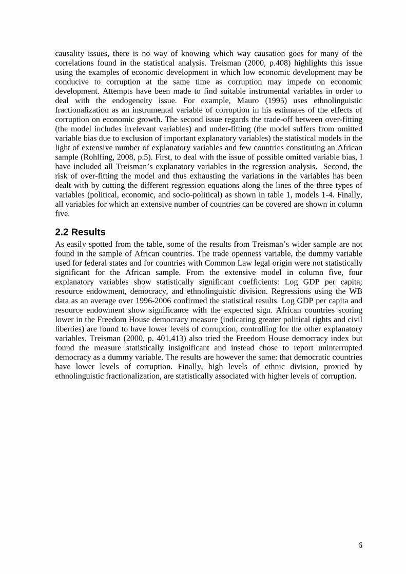
It is highly likely that causation from national income, trade openness, level of democracy and political instability, to corruption goes both ways and without feasible instrumental variables the results can only be read as correlation but not causation. Of course, some of the variables included in the models – such as colonial history, religious composition, and ethnic division – are most definitely exogenous. The only variable among that type which shows statistical significance is ethnolinguistic division, which can be read as evidence that more ethnically divided African countries have, on average, higher levels of perceived corruption. In terms of resource endowment, which also shows statistical significance, there is a possibility of reverse causality since this variable does not measure the availability of natural resources per se but instead the share of natural resource export to total export. Figure 1 below shows how well the 10 explanatory variables from regression equation five are able to predict the corruption scores for each of the countries making up the African sample.

Figure 1: Model fit: regression equation 5

The regression results presented in table 1 used the World Bank’s Control of Corruption Index (WB) as dependent variable as opposed to Treisman (2000) who used Transparency International’s Corruption Perception Index (TI). The WB index spans from -2.5 to +2.5 with the greater the value the lower the corruption. The TI index spans from zero to 10 with higher numbers indicating lower levels of corruption. These two composite indices are quite closely correlated, as shown in table 2, and this may be simply due to the TI index being used to compose the WB index. Although the WB and TI indices are commonly used in cross-section regression analyses, there exist other indices claiming to capture the level of corruption across countries. Two of these indices, both expert-based, are included in table 2

9

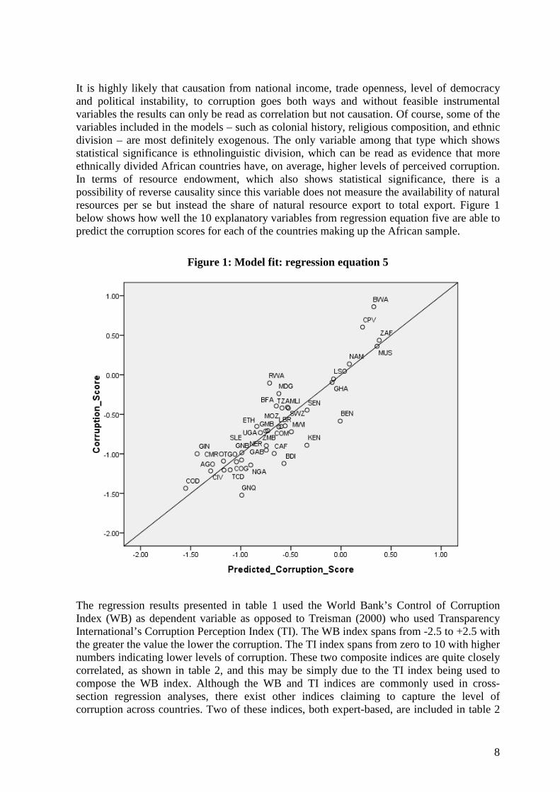
and the extended regression analysis presented in table 3. The United Nations Economic Commission for Africa (UNECA) presented in its African Governance Report 2005 the result from expert panels across 24 Sub-Saharan African countries on corruption control and various other governance issues. The higher the index value, the lower the level of corruption. The correlations between this index and the WB and the TI indices are lower (R-square 0.68 and 0.67). The last corruption index shown in table 2, International Country Risk Group index (ICRG), is also expert-based and comes from the for-profit organization Political Risk Service. This index spans from zero to 6 where higher values indicates lower levels of perceived corruption. A total of twenty-nine African countries are included in this index and, as shown in table 2, it is poorly correlated with each of other three indices. Section 5 provides a more thorough discussion on the different corruption indices and what they measure. Table 2: Correlation between the different corruption indices

World Bank’s Control of Corruption Index

Transparency International’s Corruption Perception Index

UNECA Corruption Index

ICRG Corruption Index

World Bank’s Control of Corruption Index

1.00

Transparency International’s Corruption Perception Index

0.81 1.00

UNECA Corruption Index

0.68 0.67 1.00

ICRG Corruption Index

0.14 0.04 0.09 1.00

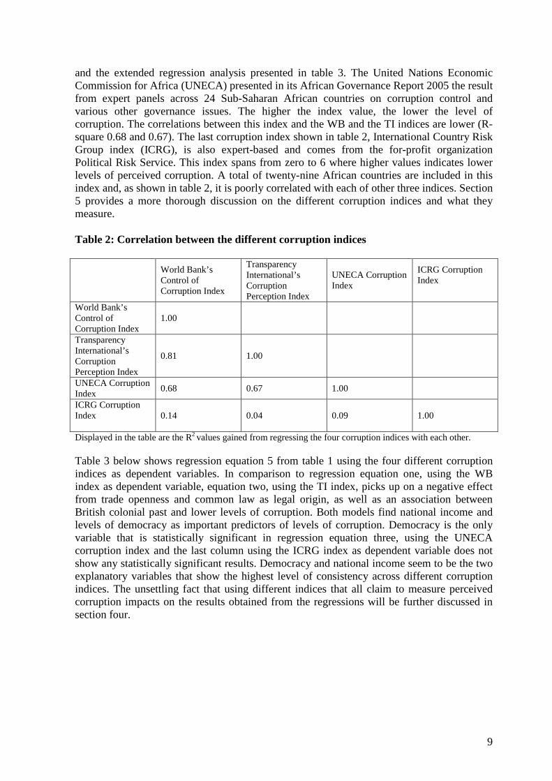
Displayed in the table are the R2 values gained from regressing the four corruption indices with each other. Table 3 below shows regression equation 5 from table 1 using the four different corruption indices as dependent variables. In comparison to regression equation one, using the WB index as dependent variable, equation two, using the TI index, picks up on a negative effect from trade openness and common law as legal origin, as well as an association between British colonial past and lower levels of corruption. Both models find national income and levels of democracy as important predictors of levels of corruption. Democracy is the only variable that is statistically significant in regression equation three, using the UNECA corruption index and the last column using the ICRG index as dependent variable does not show any statistically significant results. Democracy and national income seem to be the two explanatory variables that show the highest level of consistency across different corruption indices. The unsettling fact that using different indices that all claim to measure perceived corruption impacts on the results obtained from the regressions will be further discussed in section four.

10

Table 3: Comparison of results across different corruption indices 1: World Bank’s Control of

Corruption Index 2: Transparency International’s Corruption Perception Index

3: UNECA Corruption Index

4: ICRG Corruption Index

Log GDP per capita PPP

.3057721* (1.85)

.6878389*** (2.78)

9.922839 (1.53)

.049104 (0.07)

Import (% of GDP)

-.0043658 (-1.20)

-.0104132* (-1.86)

.0344666 (0.29)

.0037326 (0.21)

Resource endowment (hydrocarbon and/or mineral exports)

-.0035232* (-1.96)

-.0026987 (-1.03)

.0006831 (0.01)

-.0012525 (-0.22)

Democracy

-.2367484*** (-5.58)

-.3145001*** (-4.42)

-4.168089*** (-2.92)

-.1610708 (-0.89)

Political instability (government turnover)

-.6368004 (-1.47)

-.7563199 (-0.94)

-11.56323 (-0.76)

-.4316798 (-0.27)

Legal origin, 1=common law -.0003507 (-0.00)

-1.000585* (-1.71)

5.798936 (0.51)

.019978 (0.04)

Former British colony

.0768888 (0.20)

1.101645* (1.87)

-6.170568 (-0.57)

Percent protestant

.004667 (1.17)

.0091566 (1.55)

.1099681 (0.70)

.000863 (0.04)

Federal

.1464867 (0.71)

.0977214 (0.33)

-1.644415 (-0.32)

-.573892 (-1.04)

Ethnolinguistic division

-.7822665*** (-2.64)

-.7665913 (-1.66)

-2.939588 (-0.26)

.9474223 (0.60)

Constant

.1695511 (0.22)

2.831305** (2.49)

31.25803 (1.09)

2.012709 (0.61)

R-square (adjusted)

0.67 0.70 0.46 -0.31

No. of observations

39 36 24 26

Dependent variables are the World Bank Control of Corruption Index (2006); Transparency International’s Corruption Perception Index (2006); UNECA’s Corruption Index (2005), and the ICRG’s Corruption Index (2003). T-statistics are in brackets and ***, **, and * indicates p < 0.01; 0.05; and 0.1 respectively.

11

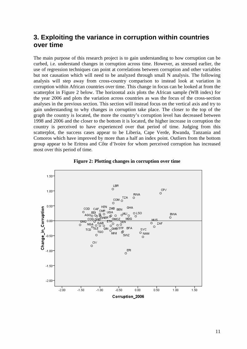
3. Exploiting the variance in corruption within countries over time The main purpose of this research project is to gain understanding to how corruption can be curbed, i.e. understand changes in corruption across time. However, as stressed earlier, the use of regression techniques can point at correlations between corruption and other variables but not causation which will need to be analyzed through small N analysis. The following analysis will step away from cross-country comparison to instead look at variation in corruption within African countries over time. This change in focus can be looked at from the scatterplot in Figure 2 below. The horizontal axis plots the African sample (WB index) for the year 2006 and plots the variation across countries as was the focus of the cross-section analyses in the previous section. This section will instead focus on the vertical axis and try to gain understanding to why changes in corruption take place. The closer to the top of the graph the country is located, the more the country’s corruption level has decreased between 1998 and 2006 and the closer to the bottom it is located, the higher increase in corruption the country is perceived to have experienced over that period of time. Judging from this scatterplot, the success cases appear to be Liberia, Cape Verde, Rwanda, Tanzania and Comoros which have improved by more than a half an index point. Outliers from the bottom group appear to be Eritrea and Côte d’Ivoire for whom perceived corruption has increased most over this period of time.

Figure 2: Plotting changes in corruption over time

12

3.1 Explanatory variables and data The panel regressions will continue using the explanatory variables reviewed in the previous section with a few changes. The panel regressions use as dependent variable the ICRG index (1985-2003) and the WB index (1998-2006: every second year until 2002). To my knowledge, there are only two previous pieces of research that use panel regressions to gain understanding to why changes in levels of corruption occur and both use the ICRG corruption data. Littvay’s (2006) study uses the time-series equivalents of Treisman’s (2000) variables although it primarily concerns the correlation and causation between levels of democracy and corruption. The sample size of this study is large and contains all countries for which data is available. Olofsgård and Zahran (2007) use panel regressions to look for possible correlation between times of change in corruption and political and economic reforms and use techniques borrowed form the literature on growth acceleration to find countries which have undergone enough sustainable changes in corruption levels to be of analytical interest. Some of the variables used in the previous cross-section regressions have had to be manipulated to fit the panel regressions. Log GDP per capita, import as share of GDP, and the proxy for democracy remain the same apart from entering the regressions on an annual basis. The political stability indicator is proxied for the ICRG regression specification on data from the International Country Risk Group. According to its data guide, the government stability indicator measures “the government’s ability to carry out its declared program(s), and its ability to stay in office”, and the higher the score the greater the stability. For the WB regression specification, political stability is proxied by the World Bank’s Political Instability and Violence index which is part of the World Bank Governance Indicators. Higher values indicate less political instability and violence. Three additional variables found in the corruption literature have been added to the analysis: foreign direct investment (FDI), following Hyden (2008); development aid dependency, following Svensson (1999) and Knack (1999); and economic growth, in accordance with Olofsgård and Zahran (2007). Data for all three variables are gathered from World Development Indicators online. With regards to foreign investment, Hyden (2008, p.15) mentions that foreign investors, by being closer to the world market, may demand better institutional conditions and thus have the effect of decreasing corruption. The opposite expectation, i.e. that FDI is negatively correlated with corruption, is also plausible based on the argument that the inflow of money leads to more opportunities for corruption. A similar ‘windfall’ argument is attached to development aid and Svensson (1999), using quantitative analysis, finds that development aid is negatively correlated with corruption. Knack (1999) also finds that high level of aid dependency correlates with high levels of corruption. With regards to the economic growth measure, Olofsgård and Zahran (2007, p.4) argue that economic booms may fuel corruption in the short run. However, this variable may be troublesome due to the high volatility of growth rates across time in the African sample, a point argued by Pritchett (2000, p.222). Table 4 below shows the results from the panel regression analyses. The time-invariant socio-political variables added to the cross-section regression equations in section three and other country-specific characteristics have in the panel regressions been controlled for by including country fixed effects.

13

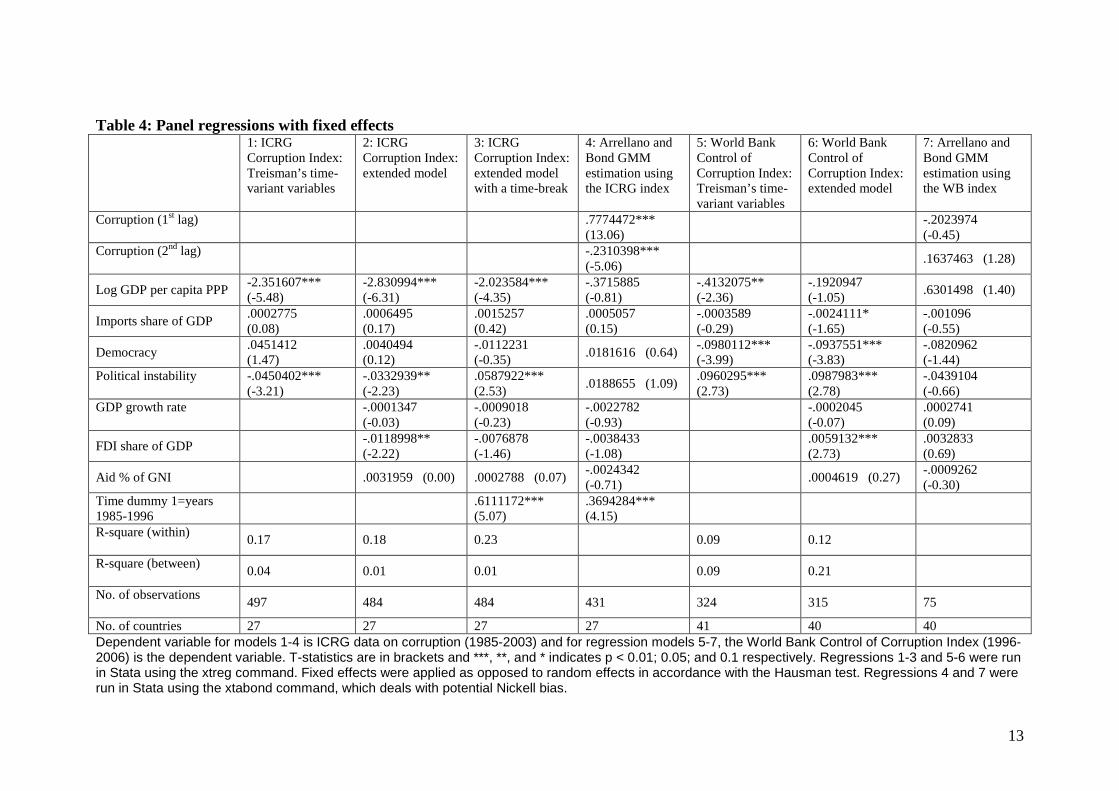
Table 4: Panel regressions with fixed effects

1: ICRG Corruption Index: Treisman’s time-variant variables

2: ICRG Corruption Index: extended model

3: ICRG Corruption Index: extended model with a time-break

4: Arrellano and Bond GMM estimation using the ICRG index

5: World Bank Control of Corruption Index: Treisman’s time-variant variables

6: World Bank Control of Corruption Index: extended model

7: Arrellano and Bond GMM estimation using the WB index

Corruption (1st lag)

.7774472*** (13.06)

-.2023974 (-0.45)

Corruption (2nd lag)

-.2310398*** (-5.06)

.1637463 (1.28)

Log GDP per capita PPP -2.351607*** (-5.48)

-2.830994*** (-6.31)

-2.023584*** (-4.35)

-.3715885 (-0.81)

-.4132075** (-2.36)

-.1920947 (-1.05)

.6301498 (1.40)

Imports share of GDP .0002775 (0.08)

.0006495 (0.17)

.0015257 (0.42)

.0005057 (0.15)

-.0003589 (-0.29)

-.0024111* (-1.65)

-.001096 (-0.55)

Democracy .0451412 (1.47)

.0040494 (0.12)

-.0112231 (-0.35)

.0181616 (0.64) -.0980112*** (-3.99)

-.0937551*** (-3.83)

-.0820962 (-1.44)

Political instability

-.0450402*** (-3.21)

-.0332939** (-2.23)

.0587922*** (2.53)

.0188655 (1.09) .0960295*** (2.73)

.0987983*** (2.78)

-.0439104 (-0.66)

GDP growth rate

-.0001347 (-0.03)

-.0009018 (-0.23)

-.0022782 (-0.93)

-.0002045 (-0.07)

.0002741 (0.09)

FDI share of GDP -.0118998** (-2.22)

-.0076878 (-1.46)

-.0038433 (-1.08)

.0059132*** (2.73)

.0032833 (0.69)

Aid % of GNI .0031959 (0.00) .0002788 (0.07) -.0024342 (-0.71)

.0004619 (0.27) -.0009262 (-0.30)

Time dummy 1=years 1985-1996

.6111172*** (5.07)

.3694284*** (4.15)

R-square (within)

0.17 0.18 0.23 0.09 0.12

R-square (between)

0.04 0.01 0.01 0.09 0.21

No. of observations

497 484 484 431 324 315 75

No. of countries 27 27 27 27 41 40 40 Dependent variable for models 1-4 is ICRG data on corruption (1985-2003) and for regression models 5-7, the World Bank Control of Corruption Index (1996-2006) is the dependent variable. T-statistics are in brackets and ***, **, and * indicates p < 0.01; 0.05; and 0.1 respectively. Regressions 1-3 and 5-6 were run in Stata using the xtreg command. Fixed effects were applied as opposed to random effects in accordance with the Hausman test. Regressions 4 and 7 were run in Stata using the xtabond command, which deals with potential Nickell bias.

14

3.2 Results From the cross-section regression analyses in section two, it was shown that, on average, more democratic and richer African countries have lower levels of corruption ceteris paribus. However, what is of real interest, especially for policy purpose, is understanding how corruption varies over time in the same country.

Column one and five present the results from those variables used by Treisman (2000) which are suitable to include in time series analysis, using the ICRG and the WB index respectively. Out of the four included explanatory variables, three show some statistical significance. However, the sign of the coefficients are not necessarily the same. In other words, according to the regression run with the ICRG index, a decrease in corruption is associated with a worsening of political stability. According to the regression run with the WB index, a decrease in corruption is associated with an improvement in both democracy and political stability. These unsettling results are corrected for the ICRG data in column three. From the ICRG time series data, it was strongly apparent that earlier years corresponded to less corruption for no known reason. The breaking point in the time series was statistically found to be in 1996/97 and a dummy where 1 equals all years before 1997 was added to the regression in column three. Using this time-dummy results in the democracy and political stability variables changing signs. However, this dummy also proves to be the strongest single right hand variable in the regression equations. Section four will further elaborate on this aspect of the data and other possible concerns regarding the corruption variable. Log GDP per capita is statistically significant but has a negative sign as opposed to a positive which it had in the cross-section analyses in section two. From the inclusion of the three additional explanatory variables in columns two and six (GDP growth, FDI and aid dependency) an increase in FDI is predicted to worsen corruption using the ICRG data but is predicted to lower corruption using WB data. Changes in aid dependency and economic growth rates do not correlate with changes in levels of corruption to any statistically significant degree. In terms of model fit, none of the panel regressions explain as much variation in the dependent variable as was reached in the cross-section regression in section three, judging by the R-squares. However, the ICRG regressions have captured more within-country variation as opposed to the WB regression for which most of the explanatory power comes from the cross-country variation. Lastly, following Olofsgård and Zahran (2007), the regression equations presented in column four and seven use Arellano and Bond’s (1991) generalized method of moments (GMM) estimation technique. The GMM method is used for situations with small T and large N panels, which is mostly the case of the WB index (8 years and 41 countries); a dependent variable that is dynamic, i.e. depending on its own past realizations; and explanatory variables that are not strictly exogenous (as discussed in section 3.1). These three issues are inherently present in the data and thus justify the use of GMM estimation. The regression equation produced by the GMM model, using twice lagged dependent variable as done by Olofsgård and Zahran (2007, p.13), becomes:

itik

itkkititit xyyy ηυβαα ++++= ∑−− ,,2211

“where iυ is the time-invariant unobserved heterogeneity, which may or may not be

correlated with the regressor in the model, and itη is an i.i.d. error term.” While the ICRG

15

data was clearly persistent as shown by the lagged corruption data in column four, the GMM regression result show no significant explanatory variable except for the time-break dummy. This is not the same result as Olofsgård and Zahran (2007, p.27) who find in their extended country sample, using the ICRG corruption data, that lower levels of corruption is associated through time with higher levels of democracy, trade openness, national income, and income growth while political stability correlates negatively with corruption. The lack of results is also evident in column seven where all previous statistically significant results vanished after the introduction of the GMM method. In conclusion, panel regression analyses with corruption as dependent variable for an African sample are able to explain very little of the variation in corruption levels within countries; leaving a large percentage of the variation unexplained by the variables included as well as time invariant country-specific variables accounted for by the fixed effects. From the statistical analysis in this section, it is clear that quantitative analysis can only very poorly explain the puzzle of how corruption is curbed in an African setting and that this type of analysis ought not to be the foundation for how anti-corruption policies are drawn up. The lack of results from this statistical exercise clearly points to a lack of appropriately identified explanatory variables from previous literature and the need for re-thinking what causes corruption to vary across time. This will most appropriately be done through in-depth case studies. The lack of statistical results could, however, also be due to problems inherent in the dependent variable. The next section will provide a discussion around the statistical use of data on corruption.

4. Measuring corruption What has been largely absent from the analysis so far is a thorough look at what has constituted the dependent variables used in the regressions in sections two and three. Some critique of existing corruption – and other types of governance – indices has sprung up lately (see, for example, Arndt and Oman (2006)). Surprisingly, however, the quantitative research references used in previous sections have been very quiet about possible biases or conceptual concerns with regards to the corruption indicators used in their regression analyses. The aim of this section is to provide answers to a couple of questions regarding the data used to measure corruption that may be of crucial importance for validating the quantitative analyses in this chapter.

1. What does data on corruption actually measure? 2. How suitable are the corruption indices for cross-section as well as time-series

statistical analysis?

4.1 Conceptualizing corruption The previous two sections have used data primarily from two different corruption indices as the dependent variable, the World Bank’s Control of Corruption Index (WB) and the International Country Risk Guide (ICRG). The WB and ICRG indices are however very different in their composition: the ICRG being based on expert ratings and the WB index being a composite index of many different sources, i.e. a poll of polls. From the ICRG explanation of what the index measures it states several different focal points. These are naturally intended to capture the type of corruption that international business (the rating company’s main paying clients) is concerned with. With regards to conceptualization, the data intends to first measure the type of corruption that may impact on the political stability in the country (“excessive patronage, nepotism, job reservations, ‘favor-

16

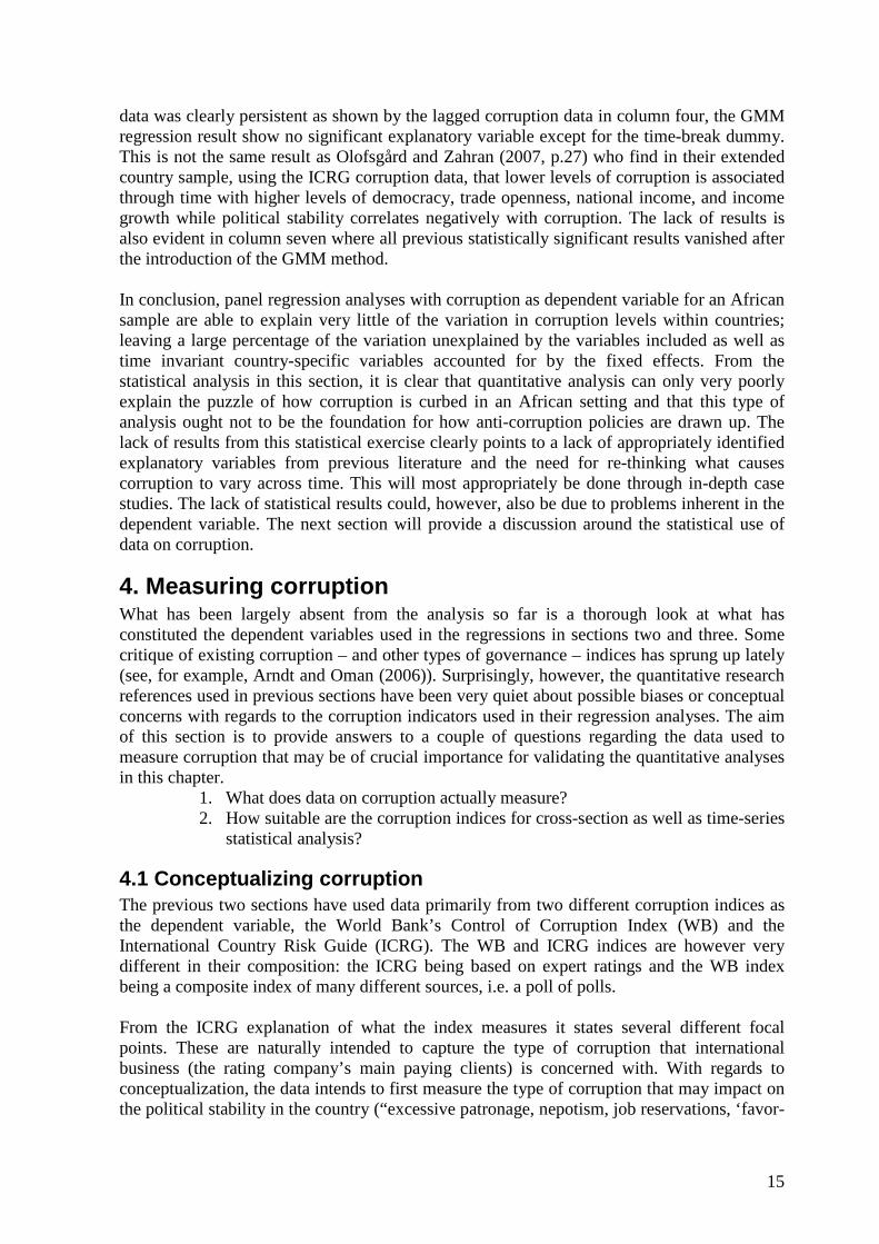
for-favors, secret party funding, and suspiciously close ties between political and business”); and second it intends to measure “demands for special payment and bribery” that directly affects foreign investors. The weights given to each of these different focal points are not reported, making the corruption measure conceptually non-precise. Also, information about what it means when a country is given a certain score, i.e., what a score of, say 5 indicates, is not disseminated. (Knack, 2007). With these issues in mind, it is difficult to know what the ICRG index points used in the previous regression analyses actually stand for. However, when it comes to conceptual uncertainty, the WB index scores much higher. The WB index provides an average for each country from many different sources, the ICRG being one of them. Like the ICRG data was geared towards the concerns of international investors, other sources of data used to form the WB index naturally have their point of reference (e.g. household data) or the interest of specific constituencies in mind. According to Søreide (2005), the pools and surveys making up the composite indices of corruption ask different corruption-related questions and thus do not necessarily cover the same issues, for example with regards to focusing on political corruption or lower-level bureaucratic corruption. “It is not clear to what extent the level of corruption reflects the frequency of corrupt acts, the damage done to society or the size of the bribes.” (Ibid, p.5). With so many different sources compiled into one average value, it means that it is impossible to know exactly what the index intent to measure, i.e. what conceptualization of corruption is represented by the data (Knack, 2007). What is usually mentioned with regards to this conceptual uncertainty as well as the perception-based nature of the data is that the data must be legitimate due to high correlation between indices (Razafindrakoto and Roubaud, 2006). For example, Olofsgård and Zahran (2007, p.9) write that “authors generally find some comfort in the fact that different measures tend to be very highly correlated.” The correlations between the four different indices used in section three were reported in table 2 and it was obvious that, at least the ICRG and the WB index were not highly correlated. This information is plotted in figure 3 below. For example, according to the ICRG index, the level of corruption is the same in Côte d’Ivoire as in Botswana while, according to the WB index, these countries are on the opposite pole in the dataset. Madagascar gets the highest score (indicating the lowest level of corruption) in the ICRG dataset but scores mediocre in the WB index. The fact that the indices do not overlap clearly leads to high level of uncertainty to what the indices actually measure and ultimately to what extent one can rely on quantitative analysis to understand corruption, cross-country and through time. This point will be discussed further in the next section.

17

Figure 3: Correlation between the WB and ICRG indices (rescaled for the year 2003)

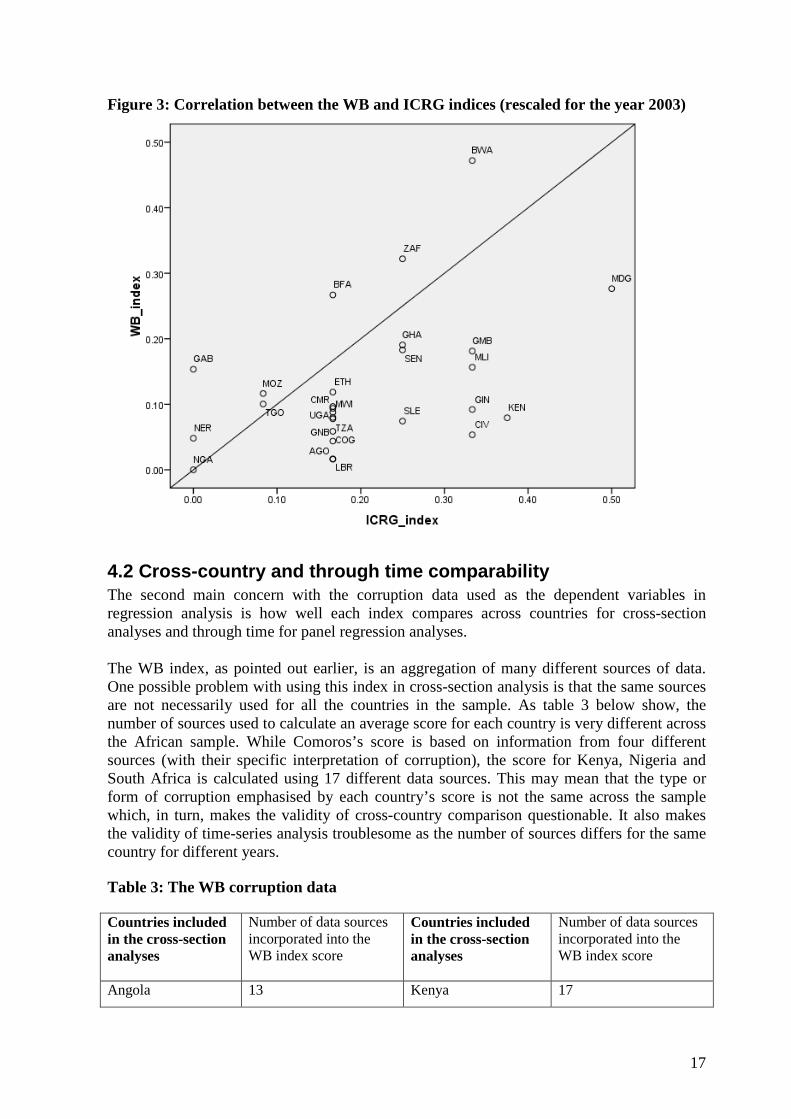
4.2 Cross-country and through time comparability The second main concern with the corruption data used as the dependent variables in regression analysis is how well each index compares across countries for cross-section analyses and through time for panel regression analyses. The WB index, as pointed out earlier, is an aggregation of many different sources of data. One possible problem with using this index in cross-section analysis is that the same sources are not necessarily used for all the countries in the sample. As table 3 below show, the number of sources used to calculate an average score for each country is very different across the African sample. While Comoros’s score is based on information from four different sources (with their specific interpretation of corruption), the score for Kenya, Nigeria and South Africa is calculated using 17 different data sources. This may mean that the type or form of corruption emphasised by each country’s score is not the same across the sample which, in turn, makes the validity of cross-country comparison questionable. It also makes the validity of time-series analysis troublesome as the number of sources differs for the same country for different years. Table 3: The WB corruption data Countries included in the cross-section analyses

Number of data sources incorporated into the WB index score

Countries included in the cross-section analyses

Number of data sources incorporated into the WB index score

Angola 13 Kenya 17

18

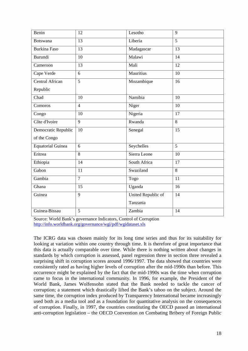
Benin 12 Lesotho 9

Botswana 13 Liberia 5

Burkina Faso 13 Madagascar 13

Burundi 10 Malawi 14

Cameroon 13 Mali 12

Cape Verde 6 Mauritius 10

Central African

Republic

5 Mozambique 16

Chad 10 Namibia 10

Comoros 4 Niger 10

Congo 10 Nigeria 17

Côte d'Ivoire 9 Rwanda 8

Democratic Republic

of the Congo

10 Senegal 15

Equatorial Guinea 6 Seychelles 5

Eritrea 8 Sierra Leone 10

Ethiopia 14 South Africa 17

Gabon 11 Swaziland 8

Gambia 7 Togo 11

Ghana 15 Uganda 16

Guinea 9 United Republic of

Tanzania

14

Guinea-Bissau 5 Zambia 14

Source: World Bank’s governance Indicators, Control of Corruption http://info.worldbank.org/governance/wgi/pdf/wgidataset.xls

The ICRG data was chosen mainly for its long time series and thus for its suitability for looking at variation within one country through time. It is therefore of great importance that this data is actually comparable over time. While there is nothing written about changes in standards by which corruption is assessed, panel regression three in section three revealed a surprising shift in corruption scores around 1996/1997. The data showed that countries were consistently rated as having higher levels of corruption after the mid-1990s than before. This occurrence might be explained by the fact that the mid-1990s was the time when corruption came to focus in the international community. In 1996, for example, the President of the World Bank, James Wolfensohn stated that the Bank needed to tackle the cancer of corruption; a statement which drastically lifted the Bank’s taboo on the subject. Around the same time, the corruption index produced by Transparency International became increasingly used both as a media tool and as a foundation for quantitative analysis on the consequences of corruption. Finally, in 1997, the countries constituting the OECD passed an international anti-corruption legislation – the OECD Convention on Combating Bribery of Foreign Public

19

Officials in International Business Transactions. This means that the unaccounted for break in the data in the mid-1990s may be due to those experts rating the countries having glanced at the newly available and highly disseminated index from Transparency International and made their scoring accordingly. It may also mean that the perception of corruption changed in accordance with its elevated focus from the international community and was judged harder by those producing the country scores. Whatever the reason for this break in the time series, the fact that it is there damages the comparability of corruption through time by showing that change has occurred within countries while this may not mirror real change in corruption. Ultimately such concerns about the comparability though time raises questions about the findings from the panel regression.

5. Conclusion This chapter has used quantitative analysis, as a first step of the nested analysis research method, to test the relevance for Africa of what previous literature has asserted in terms of correlation between corruption and a set of explanatory variables. In accordance with Lieberman’s (2005) nested analysis approach, the statistical results, or lack thereof, further provide a way forward in terms of case selection and approach to subsequent in-depth case studies. The use of statistical analysis to look at corruption – what causes it and what are the consequences of its existence – have rapidly emerged in the last decade since corruption became increasingly quantified through perception-based indices. What most studies do, however, is to incorporate all countries for which data exists. The added value of this study has instead been to evaluate previous statistical findings in the exclusive light of the African continent. Another added value has been the focus of within-country variation in corruption as opposed to the common statistical approach of looking across countries. Section two provided a list of explanatory variables known in the literature to have impacts on corruption. This list was taken from the seminal research paper by Treisman (2000) who looked at the correlates of perceived corruption from a sample which aimed at covering the entire world, relying on cross-section regression analysis. The findings from the exclusively African sample, adopting Treisman’s methods, show quite different results from those obtained by Treisman. According to his estimates, lower corruption correlates with higher national income; openness to trade; many years of uninterrupted democracy; being former British colony or Britain itself; having a unitary as opposed to federal state system; and finally, having high percentage of protestants living in the country. From the findings presented in table 1 for Africa, it shows that between-country variation in perceived corruption is correlates with levels of democracy and national income. All else being equal, African countries scoring better on Freedom House democracy index and having higher income per capita have on average lower levels of corruption. The findings also show that, ceteris paribus, heavy economic reliance on natural resources and degrees of ethnic diversity play a role in explaining cross-country variation in corruption for the African sample. Section three took the analysis from section two further by asking the data to provide statistical answers to the question of under what conditions corruption vary within African countries over time. The approach used to elaborate on this question was the use of panel regression techniques and the regression equations were built upon those variables found in Treisman (2000) as well as a few other variables gathered from recent literature. Preliminary regression results showed correlation between increased political stability and improvements

20

in the levels of corruption, and correlation between augmented income and worsening of corruption. In the case of foreign investment, the different models showed very different results. However, when accounting for endogeneity bias; large N and small T; and slow moving dependent variable, using the GMM method, all the statistical results disappeared. This means that from the statistical approaches used it is impossible to single out variables that may explain why corruption would vary within African countries over time. From the manual of Lieberman’s (2005) nested analysis method, a lack of result, such as that found in section three prescribes a model-building and inductive approach to subsequent in-depth case study analysis with a Y-centred basis for case selection. Lastly, this chapter has critically examined the data used to quantitatively capture levels of corruption in Africa and has highlighted certain problems which may be serious enough to have implications for how much can be gained from statistical analysis using corruption indices. What this analysis has pointed to is that, due to concerns about the quality of corruption data as well as an inability to find statistically significant correlations of within-country variations in corruption by applying those variables known in the literature and used in anti-corruption policy-making; the answer to the research question must be approached using a different research method. The model-building small N analysis will thus have to shoulder a larger analytical weight.

21

References

Arellano, M. and S. Bond (1991) Some Tests of Specification for Panel Data: Monte Carlo Evidence and an Application to Employment Equations, The Review of Economic Studies, 58, pp.277-297 Arndt, C. and C. Oman (2006) Uses and Abuses of Governance Indicators, Development Centre Studies, Organisation of Economic Cooperation and Development, Paris Baliamounte-Lutz, M. and L. Ndikumana, Corruption and Growth in African Countries: Exploring the Investment Channel, United Nations Economics Commission for Africa, http://www.uneca.org/aec/documents/Mina%20Baliamoune-Lutz_%20Leonce%20Ndikumana.pdf Coupet, E. Jr. (2003) Investment and Corruption: A Look at Causality, Journal of the Academy of Business and Economics http://findarticles.com/p/articles/mi_m0OGT/is_2_1/ai_113563602 Dreher, A. and Herzfeld, T. (2005) The Economic Cost of Corruption: a Survey and New Evidence, EconWPA June 506, http://econwpa.wustl.edu/eps/pe/papers/0506/0506001.pdf Easterly, W. and R. Levine (1997) Africa’s Growth Tragedy: Policies and Ethnic Divisions, Quarterly Journal of Economics, 112, 4, pp.1203-1250 Erlich, I. and F.T. Lui (1999) Bureaucratic Corruption and Endogenous Economic Growth, Journal of Political Economy, 107, 6, pp. 5270-5293 Fisman, R. and J. Svensson (2007) Are Corruption and Taxation Really Harmful to Growth? Firm Level Evidence, Journal of Development Economics, 83, pp. 63-75 Freedom House (2006) Freedom in the World 2006, Washington, D.C. Gupta, S., H. Davoodi and R. Alonso-Terme (1998), Does corruption Affect Income Inequality and Poverty?, International Monetary Fund, Working Paper WP/98/76 Hausmann, R., L. Pritchett and D. Rodrik (2005) Growth Accelerations, Journal of Economic Growth, 10, pp. 303-329 Hyden, G. (2008) Institutions, Power and Policy Outcomes in Africa, Discussion Paper No. 2, Africa Power and Politics Programme, London International Monetary Fund (2005) Guide on Resource Revenue Transparency, Washington, D.C. Jermanowski, M. (2006) Empirics of Hills, Plateaus, Mountains and Plains: A Markov-switching Approach to Growth, Journal of Development Economics, 81, pp.357-385

22

Kaufmann, D., A. Kraay and P. Zoido-Lobaton (1999) Governance Matters, World Bank, Policy Research Working Paper No. 2196, Washington, D. Knack, S. (2007) Measuring Corruption: A Critique of Indicators in Eastern Europe and Central Asia, Journal of Public Policy, 27, 3, pp. 255-291 Knack, S. (1999) Aid Dependency and the Quality of Governance: A Cross-Country Empirical Analysis, World Bank Policy Research Paper No. 2396, Washington, D.C. Lambsdorff, J. Graf (1999) Corruption in Empirical Research – A Review, Published as contribution 5 on the Website of the Internet Center for Corruption research http://www.icgg.org/downloads/contribution05_lambsdorff.pdf La Porta, R., F. López-de-Silanes, C. Pop-Eleches and A. Shleifer (2004) Judicial Checks and Balances, Journal of Political Economy, 112, 2, pp.445-470 La Porta, R., F. Lopez-de-Silanes, A. Shleifer and R.W. Vishny (1999) The Quality of Government, Journal of Economics, Law and Organization 15, 1, pp. 222-279. La Porta, R., F. Lopez-de-Silanes, A. Shleifer and R.W. Vishny (1997) Trust in Large Organizations, American Economic Association Papers and Proceedings, 87, 2, pp. 333-338 Lieberman, E.S. (2005) Nested Analysis as a Mixed-Method Strategy for Comparative Research, American Political Science Review, 99, 3, pp. 435-452 Littvay, L. (2006) Corruption and Democratic Performance, PhD Dissertation, University of Nebraska Political Science Department Mauro, P (1995) Corruption and Growth, Quarterly Journal of Economics, 60, 3, pp. 681-712 Olofsgård, A. and Z. Zahran (2007) Corruption and Political and Economic Reforms: A Structural Breaks Approach, Georgetown University, Washington, D.C. http://www9.georgetown.edu/faculty/afo2/papers/corrjune12007.pdf Poirson, H. (1998), Economic Security, Private Investment, and Growth in Developing Countries, International Monetary Fund, IMF Working Paper WP/98/4, Washington D.C. Pritchett, L. (2000) Understanding Patterns of Economic Growth: Searching for Hills Among Plateaus, Mountains, and Plains, The World Bank Economic Review 14, 2, pp. 221–250 Razafindrakoto, M. and F. Roubaud (2006) Are Inernational Databases on Corruption Reliable? A Comparison of Expert Opinion Surveys in Sub-Saharan Africa, Working paper 2006-17, Développement Institutions & Analyses de Long Terme, Paris Rohlfing, I. (2008) What You See and What You Get: Pitfalls and Principles of Nested Analysis in Comparative Research, Comparative Political Studies, 41, pp. 1492-1514 Schiavo-Campo, S. (1998) Government Employment and Pay: The Global and Regional Evidence, Public Administration and Development, 18, pp. 457-476

23

Sindzingre, A. (2002) A Comparative Analysis of African and East Asian Corruption, in A.J. Heidenheimer and M. Johnston (eds) Political Corruption: Concepts and Contexts, Third edition, Transaction Publishers, New Brunswick, N.J. Svensson, J. (1999) Foreign Aid and Rent-seeking, Journal of International Economics, 51, pp. 437-461 Svensson, J. (2003) Who Must Pay Bribes and How Much? Evidence From a Cross Section of Firms, Quarterly Journal of Economics, 118, 1, 207-230 Søreide, T. (2005) Is it Right to Rank? Limitations, Implications and Potential Improvements of Corruption Indices, Paper prepared for the IV Global Forum on Fighting Corruption, Brasilia, Brazil, 7-10 June 2005 Tanzi, V. (1994) Corruption, Government Activities, and Markets, IMF Working Paper, Washington, D.C. Tanzi, V. and H. Davoodi (1997) Corruption, Public Investment, and Growth, IMF Working Paper WP/97/139 Teorell, J., S. Holmberg and B. Rothstein (2008) The Quality of Government Dataset, version 15May08. University of Gothenburg: The Quality of Government Institute, http://www.qog.pol.gu.se Treisman, D. (2000) The Causes of Corruption: A Cross-national Study, Journal of Public Economics, 76, pp. 399-457 World Bank (2005) African Development Indicators, 2005, Washington, D.C.