towards a long-term global aerosol optical depth record: applying a
TRANSCRIPT
Atmos. Meas. Tech., 8, 4083–4110, 2015
www.atmos-meas-tech.net/8/4083/2015/
doi:10.5194/amt-8-4083-2015
© Author(s) 2015. CC Attribution 3.0 License.
Towards a long-term global aerosol optical depth record: applying a
consistent aerosol retrieval algorithm to MODIS and
VIIRS-observed reflectance
R. C. Levy1, L. A. Munchak1,2, S. Mattoo1,2, F. Patadia1,3, L. A. Remer4, and R. E. Holz5
1NASA Goddard Space Flight Center, Greenbelt, MD, USA2SSAI, Lanham, MD, USA3GESTAR, Morgan State University, Columbia, MD, USA4UMBC/JCET, Baltimore, MD, USA5SSEC, University of Wisconsin, Madison, WI, USA
Correspondence to: R. C. Levy ([email protected])
Received: 29 May 2015 – Published in Atmos. Meas. Tech. Discuss.: 8 July 2015
Revised: 11 September 2015 – Accepted: 16 September 2015 – Published: 7 October 2015
Abstract. To answer fundamental questions about aerosols
in our changing climate, we must quantify both the cur-
rent state of aerosols and how they are changing. Although
NASA’s Moderate Resolution Imaging Spectroradiometer
(MODIS) sensors have provided quantitative information
about global aerosol optical depth (AOD) for more than
a decade, this period is still too short to create an aerosol
climate data record (CDR). The Visible Infrared Imaging
Radiometer Suite (VIIRS) was launched on the Suomi-NPP
satellite in late 2011, with additional copies planned for fu-
ture satellites. Can the MODIS aerosol data record be contin-
ued with VIIRS to create a consistent CDR? When compared
to ground-based AERONET data, the VIIRS Environmen-
tal Data Record (V_EDR) has similar validation statistics
as the MODIS Collection 6 (M_C6) product. However, the
V_EDR and M_C6 are offset in regards to global AOD mag-
nitudes, and tend to provide different maps of 0.55 µm AOD
and 0.55/0.86 µm-based Ångström Exponent (AE). One rea-
son is that the retrieval algorithms are different. Using the
Intermediate File Format (IFF) for both MODIS and VIIRS
data, we have tested whether we can apply a single MODIS-
like (ML) dark-target algorithm on both sensors that leads to
product convergence. Except for catering the radiative trans-
fer and aerosol lookup tables to each sensor’s specific wave-
length bands, the ML algorithm is the same for both. We
run the ML algorithm on both sensors between March 2012
and May 2014, and compare monthly mean AOD time se-
ries with each other and with M_C6 and V_EDR products.
Focusing on the March–April–May (MAM) 2013 period, we
compared additional statistics that include global and grid-
ded 1◦× 1◦ AOD and AE, histograms, sampling frequen-
cies, and collocations with ground-based AERONET. Over
land, use of the ML algorithm clearly reduces the differences
between the MODIS and VIIRS-based AOD. However, al-
though global offsets are near zero, some regional biases
remain, especially in cloud fields and over brighter surface
targets. Over ocean, use of the ML algorithm actually in-
creases the offset between VIIRS and MODIS-based AOD
(to ∼ 0.025), while reducing the differences between AE.
We characterize algorithm retrievability through statistics of
retrieval fraction. In spite of differences between retrieved
AOD magnitudes, the ML algorithm will lead to similar de-
cisions about “whether to retrieve” on each sensor. Finally,
we discuss how issues of calibration, as well as instrument
spatial resolution may be contributing to the statistics and the
ability to create a consistent MODIS→VIIRS aerosol CDR.
1 Introduction
Aerosols are important components of the climate system,
and to answer fundamental questions about our changing cli-
mate, we must quantify the role of aerosols and how those
aerosols are changing over time. The magnitude of aerosol
forcing is difficult to assess because their loading and prop-
Published by Copernicus Publications on behalf of the European Geosciences Union.
4084 R. C. Levy et al.: Long-term global aerosol optical depth records from MODIS and VIIRS
erties vary in space and time due to intermittency of some
sources (e.g., fires, volcanoes and wind-driven dust), variable
weather that affect transport and sinks, and secular trends
caused by human policy. While the Intergovernmental Panel
on Climate Change (IPCC, 2013) has recently reported re-
duced uncertainty as to aerosol loadings and aerosol radiative
forcing effects on a global scale, it is also clear that changes
in aerosol are regional.
Whether aerosol loadings are increasing or decreasing de-
pends on location. For example, aerosols have decreased dra-
matically over eastern Europe and increased over India and
China (Chin et al., 2013). Regional aerosol changes (Zhang
and Reid, 2010) affect regional weather and local air quality,
with regional effects having global consequences, including
health (e.g., van Donkelaar et al., 2010) and economic con-
sequences (Lin et al., 2014). Therefore, it is imperative that
the community has a consistent, long-term aerosol data set,
which is global in construct, but with resolution and accuracy
sufficient to resolving regional trends.
To this end, the European Space Agency (ESA), through
their Climate Change Initiative (CCI) has recently identified
some Essential Climate Variables (ECVs) to monitor (e.g.,
Hollmann et al., 2013). One ECV is aerosol optical depth
(AOD), and the World Meteorological Organization has set
some “targets” for its measurement characteristics (GCOS,
2011). Specifically, for an AOD data set to be considered
a climate data record (CDR; e.g., NRC, 2004), it should be
able to be measured globally, every 4 h, at a resolution of 5–
10 km, with accuracy of±(0.03+10 %) and stability of 0.01
per decade. A data record of at least 30 years is a suggested
minimum for assessing global change.
The satellite aerosol record does span more than 3 decades,
if retrievals from the Advanced Very High Resolution Ra-
diometer (AVHRR) and Total Ozone Measurements (TOMS)
are considered. Yet, these instruments are limited in their
spectral and spatial information content, and also by their
lack of consistent sampling (due to changes in orbit) and
calibration. Attempts to stitch AVHRR and TOMS time se-
ries into more modern aerosol records (Mishchenko et al.,
2007a; Chan et al., 2013; Zhao et al., 2013) have helped to
derive global trends (e.g., Torres et al., 2002; Mishchenko
et al., 2007b, 2012), but their large differences in sampling
and retrieval capability make it difficult to determine regional
trends. Because the long-term aerosol variability is small
(global trends of < 0.01 decade; e.g., Hsu et al., 2012) and
usually embedded in the much larger variability associated
with the shorter (such as seasonal) time scale, we require
not only a long-term data set, but also one that is consis-
tent across instrument sampling, calibration and retrieval al-
gorithms (e.g., Weatherhead et al., 1998).
NASA’s space-borne Earth Observing System (EOS) sen-
sors have been observing the Earth system (land, oceans
and atmosphere) for over 15 years. While not meeting re-
quirements of 4 times daily observation, the EOS system ob-
serves aerosol over nearly the entire globe, with spatial and
temporal resolution sufficient to study the regional and lo-
cal scales. One of the primary instruments of EOS is the
Moderate Resolution Imaging Spectroradiometer (MODIS;
Salomonson et al., 1989), which has been flying on Terra
since December 1999 and on Aqua since May 2002. From
MODIS-observed reflectance in the visible (VIS), near-
infrared (NIR) and shortwave-IR (SWIR) wavelength re-
gions, the so-called “dark-target” (DT) aerosol algorithm
(e.g., Levy et al., 2007a, b, 2010, 2013; Remer et al., 2005,
2008) has been retrieving total aerosol optical depth (AOD)
at 0.55 µm over land and ocean at nominal 10×10 km spatial
resolution. These MODIS aerosol products are being used for
all sorts of applications, both research and routine, and re-
cently, upgraded retrieval capability has been applied to pro-
duce the Collection 6 (C6; http://modis-atmos.gsfc.nasa.gov)
time series. For a small subset of C6 DT products, Levy
et al. (2013) compared retrieved AOD to ground and ship-
based Aerosol Robotic Network (AERONET) sunphotome-
ter data (Holben et al., 1998; Smirnov et al., 2009), and de-
termined global, one-sigma expected error (EE) envelopes to
be approximately (0.04+10 %;−0.02–10 %) over ocean and
±(0.05+ 15 %) over land. This performance comes close to
the requirements as stated in the WMO document (GCOS,
2011).
Although the MODIS DT retrieval algorithm is mature and
well characterized, both MODIS instruments have exceeded
their designed lifetime. In 2006, Remer et al. (2008) showed
that Terra-MODIS and Aqua-MODIS retrieved nearly iden-
tical aerosol statistics over the ocean. Two years later, Remer
et al. (2008) found that Terra had acquired a 0.015 (12 %) off-
set from Aqua. Over land, the offset was changing with time,
suggestive of calibration drift for Terra (e.g., Levy et al.,
2010). Although steps were taken by the MODIS Calibra-
tion and Support Team (MCST) to reduce the drifting for
C6, it is expected (e.g., Levy et al., 2013) that the Terra-
Aqua offset (∼ 0.015) will remain for C6. However, Lya-
pustin et al. (2014), showed how that with even greater at-
tention to recalibration and normalization, it may be possible
to homogenize the Terra-Aqua aerosol records.
Regardless of continued re-calibration and reprocessing
of the MODIS data, MODIS will be decommissioned by
the early 2020s; there will never be a 30 year AOD record
from MODIS. However, with the launch of the Visible In-
frared Imaging Radiometer Suite (VIIRS) instrument on-
board Suomi-NPP (S-NPP) in late 2011, there is hope that
VIIRS can continue the MODIS aerosol record into the
Joint Polar Satellite System (JPSS) era. VIIRS was designed
to have similar capabilities as MODIS, with similar visi-
ble/NIR/IR spectral channels, similar spatial and temporal
resolution, and similar physics behind the retrieval algo-
rithms. In fact, NOAA (through the Interface Data Processing
Segment, IDPS) is already delivering an AOD product (Jack-
son et al., 2013) that is meeting expected accuracies, which
means performing to within similar EE envelopes stated for
the MODIS product (Liu et al., 2014). Although the VIIRS-
Atmos. Meas. Tech., 8, 4083–4110, 2015 www.atmos-meas-tech.net/8/4083/2015/
R. C. Levy et al.: Long-term global aerosol optical depth records from MODIS and VIIRS 4085
IDPS is providing a quality aerosol product especially over
ocean, the creation of a long-term AOD record not only re-
quires the availability of data, but also that the time series has
no gaps or jumps (Hollman et al., 2013).
Since any potential trend in AOD is likely to be less than
10 % per decade, and global AOD is on order of ∼ 0.2, a cli-
mate data record needs to be able to characterize AOD dif-
ferences of ∼ 0.02 or less. Using one satellite to detect this
aerosol trend requires the ability to separate out background
noise, characterize uncertainty in the retrieval and diagnose
calibration drifts. While aggregation and averaging helps to
beat down uncertainties related to noise and retrieval uncer-
tainty, averaging cannot help a calibration drift.
CDR creation is difficult with one sensor, but becomes
even more difficult when using two. The recent experience
with twin MODIS instruments with the same retrieval al-
gorithms, but on different platforms, highlights how cal-
ibration may confound the issue (e.g., Lyapustin et al.,
2014). Likewise, two instruments on the same platform (e.g.,
the Multi-angle Imaging SpectroRadiometer (MISR) and
MODIS which are both on Terra), do not agree within CDR
specifications (e.g., Liu and Mishchenko, 2008). The differ-
ences in algorithms, sampling and pixel resolution lead to
discrepancies in regional and global AOD and their trends.
MODIS and VIIRS are different instruments on different
platforms. Thus, it follows that even if the VIIRS-IDPS con-
tinues to provide a successful aerosol product, there are many
obstacles to creating a merged aerosol climate data record
from MODIS and VIIRS. These issues were discussed by
Hsu et al. (2013a), to include the following.
– sensor differences,
– calibration/characterization differences,
– sampling (orbital coverage) differences,
– retrieval algorithm differences,
– pixel selection, including cloud and other masking,
– aggregation/averaging from along-orbit products (e.g.,
Level 2), to gridded, global products (e.g., Level 3).
We cannot control the sensor differences, calibration or
how the different platforms orbit around the globe. However,
we can test whether we can homogenize the retrieval algo-
rithm, pixel selection and aggregation strategies, and thus re-
duce the differences between MODIS and VIIRS. We will
briefly describe the current MODIS and VIIRS-IDPS algo-
rithms in Sect. 2, and show that the current VIIRS-IDPS
aerosol product is significantly different from the MODIS
data set for overlapping scenes and statistics. In Sect. 3,
we develop a MODIS-like (ML) algorithm to apply to VI-
IRS spectral observations. In Sect. 4, we compare statis-
tics of our MODIS-like data to the M_C6 and VIIRS-IDPS
products, and also to ground-based sunphotometer measure-
ments. A first attempt at overlapping time series is shown
in Sect. 5. In Sect. 6, we hypothesize why complete conver-
gence may be difficult, along with further avenues to study.
Section 7 concludes that there is nothing inherent in the VI-
IRS sensor itself to prevent the creation of a long-term CDR
with a consistent algorithm to both sensors, but that a reliable
MODIS→VIIRS CDR will take much more work.
2 Comparison of MODIS-C6 and VIIRS-IDPS:
algorithm, sensor and products
2.1 Theoretical perspective
Kaufman et al. (1997a) explains how the clear-sky, top-of-
atmosphere (TOA) radiance, observed by a passive satellite,
is a combination of contributions from two sources: the atmo-
spheric path radiance (including aerosol and Rayleigh scat-
terings) and the contribution from the Earth’s surface (in-
cluding coupling between the surface and atmosphere). Re-
trieval of aerosol properties from this complicated TOA sig-
nal, therefore, requires knowledge about the surface opti-
cal properties and non-aerosol contributions. It also requires
reasonable constraints on the aerosol optical properties. To
a first approximation, the spectral reflectance at the TOA is
ρ∗ = ρa+ (T ↑T ↓ρs)/(1− [sρs
]), (1)
where ρ∗ is the reflectance at the TOA, ρa is the reflectance
of the atmosphere (also known as the path radiance), ρs is
the surface reflectance, s is the upscattering ratio, and T ↑
and T ↓ are the atmospheric transmissions (up and down) of
the surface reflectance. Except for s, all of these terms have
angular and wavelength dependence. Except for the surface
reflectance, all terms depend on the aerosol type and column
loading. The path radiance term also includes contributions
from Rayleigh (molecular) scattering.
Equation (1) is the basis of aerosol remote sensing for
MODIS, but there are many different approaches to apply-
ing this equation. Although there are many additional algo-
rithms, Table 1 lists three of the aerosol algorithms developed
and now currently used for retrieval aerosol properties from
MODIS.
The first two of these algorithms we denote as dark-
target (DT) algorithms, which are separated into over ocean
(DT_O; Tanré et al., 1997; Remer et al., 2005; Levy et al.,
2013) and over land (DT_L; Kaufman et al., 1997a; Re-
mer et al., 2005; Levy et al., 2007a, b, 2013). Both are ex-
plicit aerosol retrieval algorithms that result in aerosol prod-
ucts that are packaged and presented as parameters within
standard Terra (MOD04) or Aqua (MYD04) aerosol product
files (collectively denoted as MxD04). These algorithms are
“dark-target” because they are used for scenes where Earth’s
surface has low reflectance (is dark) in selected VIS, NIR
and SWIR wavelengths. These wavelengths are also in win-
dow regions of the atmosphere (have small gas absorption).
Since the surface reflectance is relatively small, the aerosol
www.atmos-meas-tech.net/8/4083/2015/ Atmos. Meas. Tech., 8, 4083–4110, 2015

4086 R. C. Levy et al.: Long-term global aerosol optical depth records from MODIS and VIIRS
Table 1. Three MODIS products and their references.
Index MODIS Geophysical MODIS L2 References
procedure parameters product name
DT_O Dark-target aerosol AOD, fine fraction MxD04 Tanré et al. (1997);
over ocean Remer et al. (2005)
DT_L Dark-target aerosol AOD MxD04 Kaufman et al. (1997);
over land Remer et al. (2005);
Levy et al. (2007a, b)
AC_L Atmospheric Surface reflectance MxD09 Vermote et al. (1997);
correction over land Vermote and Kotchenova (2008)
signal is a major component of the TOA signal. The portion
of the TOA signal attributed to aerosol can be estimated with
radiative transfer, and using lookup tables (LUTs), one can
retrieve the properties of the aerosol (AOD and aerosol type
or model) that contributed to this aerosol portion. In this pro-
cess, by iterating through increasing values of AOD and vari-
ous candidate aerosol models, the algorithm finds an optimal
solution that best matches the reflectance measurements to
the theoretical (LUT) values at the TOA.
The DT algorithm constrains the surface (either implic-
itly or explicitly). With DT_O, the surface contribution is
modeled explicitly (Ahmad and Fraser, 1982) as an addi-
tion of a flat dark ocean (nearly black in NIR and SWIR
channels), plus some water leaving radiance (in VIS chan-
nels), plus whitecaps, foam and glitter (e.g., Cox and Munk,
1954; Koepke, 1984). Over land, although the land surface
reflectance varies greatly with season and location, Kauf-
man et al. (1997b) found that, over vegetation and dark soils,
the surface reflectance in a blue wavelength is approximately
equal to half that in a red wavelength, which is in turn half
that of a SWIR wavelength (e.g., near 2.1 µm). This land sur-
face parameterization is applied to the DT_L to constrain
systems of equations (one for each wavelength). For both
DT algorithms, the goodness of fit is judged by the closeness
between computed and measured TOA reflectance in the se-
lected channels.
The third algorithm (AC_L; Vermote et al., 1997, 2002)
listed in Table 1 derives aerosol information internally and
uses the aerosol information for deriving atmospherically
corrected surface products (the “MxD09” product). The
AC_L algorithm used for MxD09 shares a common devel-
oper heritage with the DT_L used for MxD04 (note over-
lap of authors between Kaufman et al., 1997a and Vermote
et al., 1997). However, instead of solving for the TOA re-
flectance ρ∗ as the DT algorithm, it inverts the equation and
solves for the surface reflectance, ρs. The comparison be-
tween the derived and expected spectral surface reflectance
determines the best solution. Since 1997, the AC_L and
DT_L algorithms and products have diverged because of dif-
ferent needs. DT_L tries to derive aerosol properties (Remer
et al., 2005; Levy et al., 2007a, b), regardless of surface con-
ditions, and AC_L tries to derive land properties regardless
of atmosphere conditions (Vermote and Kotchenova, 2008).
DT_L must retrieve aerosol at all aerosol loadings, includ-
ing very heavy aerosol events, while AC_L can choose to ig-
nore these heavy events to ensure accurate surface retrievals.
Theoretically, the resulting AOD and aerosol model could be
similar to that of a DT algorithm, but in practice, this may
not be the case.
2.2 A short history
The MODIS DT algorithm has been updated since formula-
tion in the 1990s and implementation on Terra and Aqua. In
MODIS terminology, a stable combination of algorithm ver-
sion and product version is known as a Collection, which we
refer to by CX where X is a number. C2 began at launch, C3
began soon after, and C4 denoted the first attempt to com-
bine forward processing and reprocessing of old data. By
late 2005 the DT_L and DT_O aerosol retrieval algorithms
became stable. The C5 aerosol data set (MxD04) was pro-
cessed with identical DT aerosol retrieval algorithms on both
Terra and Aqua, theoretically leading to a consistent MODIS
aerosol data record. However, as explained in the introduc-
tion, using a common algorithm for the entire data mission
did not ensure a CDR-quality data set. Differences in cali-
bration crept in, leading to artificial trending of AOD. Start-
ing in 2014, the entire MODIS mission is being processed
again with updated algorithms. Corrections to calibration
have been applied, and the products are known as Collec-
tion 6 (C6; Levy et al., 2013). The MODIS C6 (M_C6) data
cover the entirety of the MODIS mission, including temporal
overlap with VIIRS.
Development for the VIIRS algorithms over land and
ocean (V_L and V_O) began in the early 2000s, concurrent
with earlier versions of the MODIS algorithms. At this point
the personnel overlap between algorithm teams disappeared,
causing the algorithms to diverge. The V_L algorithm is
a variant of the AC_L algorithm, which employs extra blue
wavelengths that help constrain aerosol type (Vermote and
Kotchenova, 2008). The V_O algorithm is directly adapted
from DT_O, but with adjustments and modifications. For ex-
ample, the spectral inversion for V_O does not use a green
Atmos. Meas. Tech., 8, 4083–4110, 2015 www.atmos-meas-tech.net/8/4083/2015/
R. C. Levy et al.: Long-term global aerosol optical depth records from MODIS and VIIRS 4087
Table 2. MODIS and VIIRS instrument specifications.
Aqua-MODIS Suomi NPP-VIIRS
Orbit altitude 705 km 824 km
Equator crossing time 13:30 LT 13:30 LT
Swath width 2330 km 3040 km
Sensor zenith angle range ±64◦ ±70◦
Wavelength bands 36 bands (20 in solar spectrum) 22 bands (15 in solar spectrum)
Pixel size, nadir 1.0/0.50/0.25 km 0.75/0.375 km
Pixel growth factor, edge of scan 4.8× 2.0 1.6× 1.6
Bow-tie effects Yes Decreased
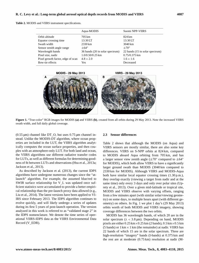
Figure 1. “True-color” RGB images for MODIS (a) and VIIRS (b), created from all orbits during 29 May 2013. Note the increased VIIRS
swath width, and full daily global coverage.
(0.55 µm) channel like DT_O, but uses 0.75 µm channel in-
stead. Unlike the MODIS-DT algorithm, where ocean prop-
erties are included in the LUT, the VIIRS algorithm analyt-
ically computes the ocean surface properties, and then cou-
ples with an atmosphere-only LUT. For both land and ocean,
the VIIRS algorithms use different radiative transfer codes
for LUTs, as well as different formulas for determining good-
ness of fit between LUTs and observations (Hsu et al., 2013a;
Jackson et al., 2013).
As described by Jackson et al. (2013), the current IDPS
algorithms have undergone numerous changes since the “at-
launch” algorithm. For example, the assumed blue/red to
SWIR surface relationship for V_L was updated once suf-
ficient statistics were accumulated to provide a better empiri-
cal relationship than the pre-launch proxy data allowed (e.g.,
Liu et al., 2014). The latest versions have been applied to VI-
IRS since February 2013. The IDPS algorithm continues to
evolve quickly, and will likely undergo a series of updates
during its first 5 years of post-launch operation. The version
analyzed in this work is referred to as “validated stage 2” in
the IDPS nomenclature. We denote the time series of oper-
ational VIIRS-IDPS data as the VIIRS Environmental Data
Record (V_EDR).
2.3 Sensor differences
Table 2 shows that although the MODIS (on Aqua) and
VIIRS sensors are mostly similar, there are also some key
differences. VIIRS on S-NPP orbits at 824 km, compared
to MODIS aboard Aqua orbiting from 705 km, and has
a larger sensor view zenith angle (±70◦ compared to ±64◦
for MODIS), which both allow VIIRS to have a significantly
larger ground swath than MODIS (3040 km compared to
2330 km for MODIS). Although VIIRS and MODIS-Aqua
both have similar local equator crossing times (1.30 p.m.),
they overlap exactly (viewing a target from nadir and at the
same time) only every 3 days and only over polar sites (Up-
rety et al., 2013). Over a given mid-latitude or tropical site,
MODIS and VIIRS observe with varying offsets, ranging
from a few minutes apart (with similar solar/viewing geome-
try) on some days, to multiple hours apart (with different ge-
ometry) on others. In Fig. 1 we plot 1 day’s (29 May 2013)
orbits worth of both MODIS and VIIRS imagery, showing
coverage differences between the two orbits.
MODIS has 36 wavelength bands, of which 20 are in the
solar spectrum (λ < 3.8 µm). Depending on band, MODIS
pixels are either 0.25km×0.25 km (2 bands), 0.5km×0.5 km
(5 bands) or 1km×1 km (the remainder) at nadir. VIIRS has
22 bands of which 15 are in the solar spectrum. Three are
high-resolution “imagery” bands (I-bands) at 0.375 km and
the rest are at moderate (0.75 km) resolution at nadir (M-
www.atmos-meas-tech.net/8/4083/2015/ Atmos. Meas. Tech., 8, 4083–4110, 2015
4088 R. C. Levy et al.: Long-term global aerosol optical depth records from MODIS and VIIRS
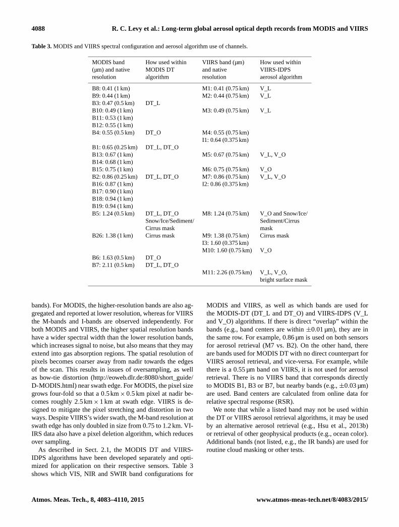
Table 3. MODIS and VIIRS spectral configuration and aerosol algorithm use of channels.
MODIS band How used within VIIRS band (µm) How used within
(µm) and native MODIS DT and native VIIRS-IDPS
resolution algorithm resolution aerosol algorithm
B8: 0.41 (1 km) M1: 0.41 (0.75 km) V_L
B9: 0.44 (1 km) M2: 0.44 (0.75 km) V_L
B3: 0.47 (0.5 km) DT_L
B10: 0.49 (1 km) M3: 0.49 (0.75 km) V_L
B11: 0.53 (1 km)
B12: 0.55 (1 km)
B4: 0.55 (0.5 km) DT_O M4: 0.55 (0.75 km)
I1: 0.64 (0.375 km)
B1: 0.65 (0.25 km) DT_L, DT_O
B13: 0.67 (1 km) M5: 0.67 (0.75 km) V_L, V_O
B14: 0.68 (1 km)
B15: 0.75 (1 km) M6: 0.75 (0.75 km) V_O
B2: 0.86 (0.25 km) DT_L, DT_O M7: 0.86 (0.75 km) V_L, V_O
B16: 0.87 (1 km) I2: 0.86 (0.375 km)
B17: 0.90 (1 km)
B18: 0.94 (1 km)
B19: 0.94 (1 km)
B5: 1.24 (0.5 km) DT_L, DT_O M8: 1.24 (0.75 km) V_O and Snow/Ice/
Snow/Ice/Sediment/ Sediment/Cirrus
Cirrus mask mask
B26: 1.38 (1 km) Cirrus mask M9: 1.38 (0.75 km) Cirrus mask
I3: 1.60 (0.375 km)
M10: 1.60 (0.75 km) V_O
B6: 1.63 (0.5 km) DT_O
B7: 2.11 (0.5 km) DT_L, DT_O
M11: 2.26 (0.75 km) V_L, V_O,
bright surface mask
bands). For MODIS, the higher-resolution bands are also ag-
gregated and reported at lower resolution, whereas for VIIRS
the M-bands and I-bands are observed independently. For
both MODIS and VIIRS, the higher spatial resolution bands
have a wider spectral width than the lower resolution bands,
which increases signal to noise, but also means that they may
extend into gas absorption regions. The spatial resolution of
pixels becomes coarser away from nadir towards the edges
of the scan. This results in issues of oversampling, as well
as bow-tie distortion (http://eoweb.dlr.de:8080/short_guide/
D-MODIS.html) near swath edge. For MODIS, the pixel size
grows four-fold so that a 0.5km× 0.5 km pixel at nadir be-
comes roughly 2.5 km× 1 km at swath edge. VIIRS is de-
signed to mitigate the pixel stretching and distortion in two
ways. Despite VIIRS’s wider swath, the M-band resolution at
swath edge has only doubled in size from 0.75 to 1.2 km. VI-
IRS data also have a pixel deletion algorithm, which reduces
over sampling.
As described in Sect. 2.1, the MODIS DT and VIIRS-
IDPS algorithms have been developed separately and opti-
mized for application on their respective sensors. Table 3
shows which VIS, NIR and SWIR band configurations for
MODIS and VIIRS, as well as which bands are used for
the MODIS-DT (DT_L and DT_O) and VIIRS-IDPS (V_L
and V_O) algorithms. If there is direct “overlap” within the
bands (e.g., band centers are within ±0.01 µm), they are in
the same row. For example, 0.86 µm is used on both sensors
for aerosol retrieval (M7 vs. B2). On the other hand, there
are bands used for MODIS DT with no direct counterpart for
VIIRS aerosol retrieval, and vice-versa. For example, while
there is a 0.55 µm band on VIIRS, it is not used for aerosol
retrieval. There is no VIIRS band that corresponds directly
to MODIS B1, B3 or B7, but nearby bands (e.g., ±0.03 µm)
are used. Band centers are calculated from online data for
relative spectral response (RSR).
We note that while a listed band may not be used within
the DT or VIIRS aerosol retrieval algorithms, it may be used
by an alternative aerosol retrieval (e.g., Hsu et al., 2013b)
or retrieval of other geophysical products (e.g., ocean color).
Additional bands (not listed, e.g., the IR bands) are used for
routine cloud masking or other tests.
Atmos. Meas. Tech., 8, 4083–4110, 2015 www.atmos-meas-tech.net/8/4083/2015/

R. C. Levy et al.: Long-term global aerosol optical depth records from MODIS and VIIRS 4089
2.4 Practical differences
The MODIS DT and VIIRS-IDPS aerosol retrieval teams
have adopted different strategies for increasing the robust-
ness of their retrieved products. This includes steps to mask
pixels that are unsuitable for aerosol retrieval (e.g., clouds,
glint, etc.) as well as steps to assess confidence in the final
product.
To identify and mask clouds, the MODIS DT algorithm
combines internal spatial variability and reflectance thresh-
old tests with three thermal IR tests from the external Wis-
consin cloud mask (MxD35, e.g., Frey et al., 2008). The
VIIRS-IDPS algorithm relies on an upstream VIIRS Cloud
Mask (VCM; e.g., Vermote et al., 2014; Kopp et al., 2014)
for cloud masking. Both algorithms have their own methods
for screening out snow, ice, glint, and other pixels unsuitable
for retrieval.
Even after unambiguously unsuitable pixels are discarded,
pixel by pixel retrieval can create a noisy product (e.g., Tanré
et al., 1997). To increase signal and robustness in the product,
one could either aggregate the pixels (then do one aerosol re-
trieval), or do pixel retrievals but then average the results. The
strategy for the MODIS DT algorithm is the former, which
means it creates 20× 20 boxes of nominal 0.5 km data, and
derives an “average” spectral reflectance that represents the
nominal 10 km box. When creating this average, the masked
pixels are discarded, along with some fraction of the remain-
der, in order to ensure that the retrieval is based on appropri-
ate pixels. The retrieval is made once for a 10 km box. On
the other hand, the VIIRS-IDPS strategy is to retrieve on ev-
ery 0.75 km pixel that is not masked (e.g., clouds), known
as the intermediate product (IP). To create a final product (at
6 km resolution), the algorithm aggregates an 8× 8 box of
these 0.75 km pixels. Although the end result for both the
MODIS-DT and VIIRS-IDPS algorithms is a robust retrieval
of aerosol properties, the strategies for attaining it differ.
On MODIS, the DT algorithms’ primary products are to-
tal aerosol optical depth (AOD at 0.55 µm) over land and
ocean, plus information about particle size over ocean. This
size information is reported in a number of ways includ-
ing: fraction of AOD (at 0.55 µm) contributed by small par-
ticles known as fine mode fraction or FMF; the Ångström
exponents (AE) for two wavelength pairs (0.55/0.86 and
0.86/2.11 µm); the effective radius; and spectral AOD at
seven wavelengths. All other MODIS DT products are either
derived from these primary products or are diagnostics of the
retrieval. Note that prior to C6, MODIS also included AE
over land (0.47/0.65 µm) but was dropped from the product
list due to having little quantitative value (e.g., Levy et al.,
2013).
VIIRS produces the same basic information as MODIS:
AOD at 0.55 µm over land and ocean, plus a particle size
parameter over ocean. However, the VIIRS size parameter
over ocean is given only as an AE for the wavelength pair
0.86/1.61 µm and as spectral AOD in 11 wavelengths. There
is no effective radius product, and FMF is a diagnostic only
available at the IP level. VIIRS produces an AE over land
(0.49/0.67 µm), but preliminary validation suggests there is
no quantitative skill. We will not further discuss AE over
land.
Jackson et al. (2013) and Liu et al. (2014) discuss the con-
cepts of quality assurance (QA) as applied to the VIIRS-
IDPS algorithm, while Levy et al. (2013) discusses QA in
relation to the MODIS DT algorithm for C6. The criteria
and definitions differ, but the end result is an integer that
ranges from 0 to 3, roughly representing the range of “no
confidence” to “high confidence” in the retrieved product.
2.5 Product differences
Although the VIIRS retrieval algorithm was developed in-
dependently, the primary product of both the MODIS DT
and VIIRS-IDPS algorithms is the AOD at 0.55 µm. Liu
et al. (2014) have already performed comparison of MODIS
C5 and VIIRS-IDPS data, but since then, the MODIS algo-
rithm has been updated to C6. Therefore, we start with com-
parisons of MODIS C6 (M_C6) and VIIRS-IDPS data (the
V_EDR) products after 23 February 2013.
Figure 2 presents red–green–blue (RGB) imagery and
AOD retrieval for a near-overlapping scene over India and
the Bay of Bengal. Both MODIS and VIIRS images start at
07:35 UTC on 5 March 2013, but with ground-track sepa-
rated by about 350 km. 3.5 VIIRS 86 s granules were stitched
together to resemble one MODIS 5 min granule. The MODIS
AOD is plotted with 10 km resolution (at nadir), meeting
the quality assurance confidence (QAC) requirements for
MODIS (QAC≥ 1 over-ocean and QAC= 3 over land). The
VIIRS AOD is plotted for 6 km pixels with the VIIRS team’s
QAC recommendations (QAC= 3 for both ocean and land).
Although the surface issues and cloud patterns appear the
same for the common sampling, the retrieved AOD values are
different, especially over land. Over Bangladesh, MODIS re-
trieves much higher AOD (∼ 0.7) than VIIRS (∼ 0.4). Over
much of India, MODIS retrieves near zero values, with VI-
IRS not retrieving at all. Clearly, there are differences in
where each sensor chose to retrieve, whether due to suspi-
cion of clouds or surface issue. On the other hand, where not
impacted by glint, the coverages and magnitudes over ocean
are very similar, including both showing the tiny plume off
to the west of the Malay Peninsula.
Seasonally averaged AOD maps for March–April–May
(MAM) 2013 are shown in Fig. 3, following the aggrega-
tion strategy described in Levy et al. (2013) for calculating
monthly mean. For sufficient QAC, at least five pixels are re-
quired to create a daily mean for a given 1◦× 1◦ grid, and
at least 3 days are required to create a seasonal mean. While
3 days may not be sufficiently representative of a seasonal
mean, we assume it is for comparison purposes. Figure 4
presents scatterplots for (V_EDR vs. M_C6) of the seasonal
www.atmos-meas-tech.net/8/4083/2015/ Atmos. Meas. Tech., 8, 4083–4110, 2015

4090 R. C. Levy et al.: Long-term global aerosol optical depth records from MODIS and VIIRS
Figure 2. Overlap of MODIS and VIIRS centered on the Bay of Bengal, during a 5-minute period starting at 5 March 2013 at 07:35. (a and
b) are true-color RGB images for MODIS and VIIRS. (c and d) are retrieved QA-filtered AOD at 0.55 µm for the MODIS C6 (10 km) and
VIIRS EDR (6 km) products. AOD are plotted based on published quality assurance recommendations for each product.
means in collocated grids, where each point denotes a sea-
sonal mean calculated from both data sets.
Like the comparisons that Liu et al. (2014) show of
MODIS C5 and VIIRS AOD, we see that the overall global
patterns of AOD are similar between the two data sets. AOD
is significantly smaller in the Southern Hemisphere (both
land and ocean) for both products. There are hotspots for
both data sets in southeast Asia, central America and central
Africa. One change from the C5-based analysis is a larger
coverage for MODIS in the southern oceans, due to allow-
ing for aerosol retrieval under larger solar zenith angles.
Otherwise, except for the complex cloud/aerosol belts east
of Asia, MODIS and VIIRS seem to have converged over
ocean, even compared to Liu et al. (2014). Primarily, this is
because M_C6 has introduced wind speed dependence into
the DT_O retrieval, which had already been included in the
VIIRS-IDPS retrieval. In fact, the scatterplot (Fig. 4a) shows
near one-to-one agreement for grid cells where both M_C6
and V_EDR provide data, with coefficent of determination
R2= 0.89. Assuming the global seasonal mean to be the
simple average of retrieved grid values (no accounting for
surface area), for MAM 2013, both data sets indicate mean
AOD over ocean of ∼ 0.13.
Yet, over land, the differences remain large. Even with
the upgrades to surface reflectance relationship for MODIS
C6 (e.g., Levy et al., 2013), the AOD for V_EDR remains
much higher than MODIS (Fig. 4b). The exceptions are near
desert fringes and areas where surfaces tend to be brighter
(Fig. 3c). Most of the difference patterns are consistent with
those described by Liu et al. (2014). For collocated grid cells
with over-land AOD during MAM (Fig. 4b), R2= 0.58, and
the V_EDR product is biased high by 0.06 as compared to
M_C6. We note that the high bias of VIIRS at high north-
ern latitudes is associated with snow melt during the spring,
and that there is a planned update to the operational VIIRS
algorithm to be implemented by 2016.
Atmos. Meas. Tech., 8, 4083–4110, 2015 www.atmos-meas-tech.net/8/4083/2015/

R. C. Levy et al.: Long-term global aerosol optical depth records from MODIS and VIIRS 4091
Figure 3. Spring (March–April–May) 2013 maps (1◦×1◦) of QA-filtered mean AOD at 0.55 µm, derived from the MODIS C6 (a) and VIIRS
EDR (b) products. (c) plots the difference between (b) and (a). (d) represents the “increased” coverage of VIIRS-EDR using AOD units,
with reduced coverage plotted as black. Note that the seasonal AOD in a gridbox is the average of three monthly AODs, which in turn are
derived as the average of daily AOD within each month. Published QA-filtering for each product is followed.
MAM 2013, Ocean
0.0 0.2 0.4 0.6 0.8M_C6 0.55 µm AOD
0.0
0.2
0.4
0.6
0.8
V_ED
R 0.
55 µ
m A
OD
Y = 0.890x + 0.012N = 32476; R2 = 0.890Bias = −0.004RMSE = 0.028
A
MAM 2013, Land
0.0 0.2 0.4 0.6 0.8M_C6 0.55 µm AOD
0.0
0.2
0.4
0.6
0.8
V_ED
R 0.
55 µ
m A
OD
Y = 0.678x + 0.101N = 10049; R2 = 0.582Bias = 0.058RMSE = 0.118
B1
3
6
9
12
15
18
21
24
27
Frequency
Figure 4. Comparison of mean AOD in collocated grids from the Spring 2013 maps (e.g., Fig. 2), for ocean retrievals (a) and land re-
trievals (b). Statistics (regression equation, number of collocated grids, correlation, bias and RMSE) are provided as text in each panel.
www.atmos-meas-tech.net/8/4083/2015/ Atmos. Meas. Tech., 8, 4083–4110, 2015
4092 R. C. Levy et al.: Long-term global aerosol optical depth records from MODIS and VIIRS
3 The MODIS-like algorithm
Although both M_C6 and V_EDR products are meeting their
prescribed goals for accuracy, the differences between them
are too large to enable seamless creation of a CDR. However,
based on the experience of the ocean color community (e.g.,
Franz et al., 2005, 2012), consistent algorithms may help.
First, however, we have to create consistent input data.
3.1 The Intermediate File Format
A standard MODIS “granule” represents the swath col-
lected over 5 min (288 per day). About 138 are daylight
scenes suitable for aerosol retrieval. The combination of geo-
location (angles, whether land/sea, etc.) and calibrated ra-
diance/reflectance data are known as Level 1B (L1B) data
and are stored in Hierarchal Data Format version 4 (HDF4).
Calibrated data are separated into three files; one containing
the 0.25 km bands (bands 1 and 2; B1 and B2), the second
containing the 0.5 km bands (B3–B7, plus aggregated B1–
B2), and the third containing the 1 km bands (B8–B36, plus
aggregated B1–B7). Standard VIIRS data cover 86 s, are in
HDF5 format, and each band is contained as a separate file.
This leads to thousands of files per day, which, although an
advantage for parallel computer processing, means that the
VIIRS data are not easily used for MODIS-like processing.
To overcome some of these formatting differences, the
NASA Atmosphere Science Investigator-led Processing Sys-
tem at the University of Wisconsin (A-SIPS; http://sips.ssec.
wisc.edu/) created the Intermediate File Format (IFF) L1B
files for both MODIS and VIIRS. For VIIRS, this meant join-
ing native resolution (86 s) granules into 5-minute MODIS-
like granules, combining all M-bands and geolocation into
a single file, filling in “bowtie-deleted” pixels, and finally
archiving them in HDF4 format. The A-SIPS also created
MODIS-based IFF files that included only 1 km resolution
data (native 1 km plus aggregated B1–7 data) and similar ge-
olocation information. The IFF data are essentially a “lowest
common denominator”, reporting only data at coarsest reso-
lution (1 km for MODIS, and 0.75 km for VIIRS).
With IFF produced for both VIIRS and MODIS (e.g.,
V_IFF and M_IFF), a generic algorithm could theoretically
be applied to either one. However, since the IFF only includes
coarse resolution reflectance and geolocation data, not all in-
puts for the standard C6 algorithm are available. For exam-
ple, the Wisconsin cloud mask (Frey et al., 2008) is not in-
cluded for MODIS-IFF because the analogue for VIIRS is
still under development. Thus, the lack of high-resolution re-
flectance data and upstream infrared-based cloud informa-
tion will impact our various mask tests (clouds, ice/snow,
underwater sediments and inland water) when we compare
to standard M_C6 data. We envisioned, however, that this
would provide a more level playing field when comparing
the M_IFF and V_IFF outputs.
0
20
40
60
80
100
% R
efle
ctan
ce
DeciduousConiferSeawater
MODISVIIRSOverlap
0.5 1.0 1.5 2.0Wavelength [µm]
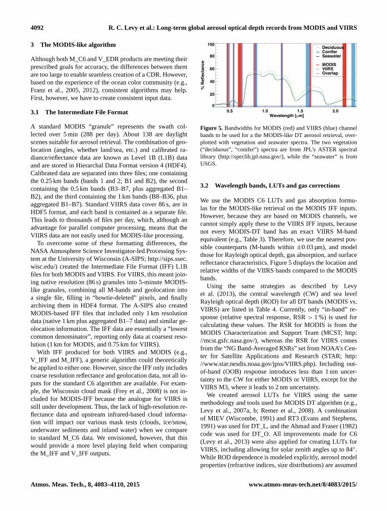
Figure 5. Bandwidths for MODIS (red) and VIIRS (blue) channel
bands to be used for a the MODIS-like DT aerosol retrieval, over-
plotted with vegetation and seawater spectra. The two vegetation
(“deciduous”, “conifer”) spectra are from JPL’s ASTER spectral
library (http://speclib.jpl.nasa.gov/), while the “seawater” is from
USGS.
3.2 Wavelength bands, LUTs and gas corrections
We use the MODIS C6 LUTs and gas absorption formu-
las for the MODIS-like retrieval on the MODIS IFF inputs.
However, because they are based on MODIS channels, we
cannot simply apply these to the VIIRS IFF inputs, because
not every MODIS-DT band has an exact VIIRS M-band
equivalent (e.g., Table 3). Therefore, we use the nearest pos-
sible counterparts (M-bands within ±0.03 µm), and model
those for Rayleigh optical depth, gas absorption, and surface
reflectance characteristics. Figure 5 displays the location and
relative widths of the VIIRS bands compared to the MODIS
bands.
Using the same strategies as described by Levy
et al. (2013), the central wavelength (CW) and sea level
Rayleigh optical depth (ROD) for all DT bands (MODIS vs.
VIIRS) are listed in Table 4. Currently, only “in-band” re-
sponse (relative spectral response, RSR > 1 %) is used for
calculating these values. The RSR for MODIS is from the
MODIS Characterization and Support Team (MCST; http:
//mcst.gsfc.nasa.gov/), whereas the RSR for VIIRS comes
from the “NG Band-Averaged RSRs” set from NOAA’s Cen-
ter for Satellite Applications and Research (STAR; http:
//www.star.nesdis.noaa.gov/jpss/VIIRS.php). Including out-
of-band (OOB) response introduces less than 1 nm uncer-
tainty to the CW for either MODIS or VIIRS, except for the
VIIRS M3, where it leads to 2 nm uncertainty.
We created aerosol LUTs for VIIRS using the same
methodology and tools used for MODIS DT algorithm (e.g.,
Levy et al., 2007a, b; Remer et al., 2008). A combination
of MIEV (Wiscombe, 1991) and RT3 (Evans and Stephens,
1991) was used for DT_L, and the Ahmad and Fraser (1982)
code was used for DT_O. All improvements made for C6
(Levy et al., 2013) were also applied for creating LUTs for
VIIRS, including allowing for solar zenith angles up to 84◦.
While ROD dependence is modeled explicitly, aerosol model
properties (refractive indices, size distributions) are assumed
Atmos. Meas. Tech., 8, 4083–4110, 2015 www.atmos-meas-tech.net/8/4083/2015/
R. C. Levy et al.: Long-term global aerosol optical depth records from MODIS and VIIRS 4093
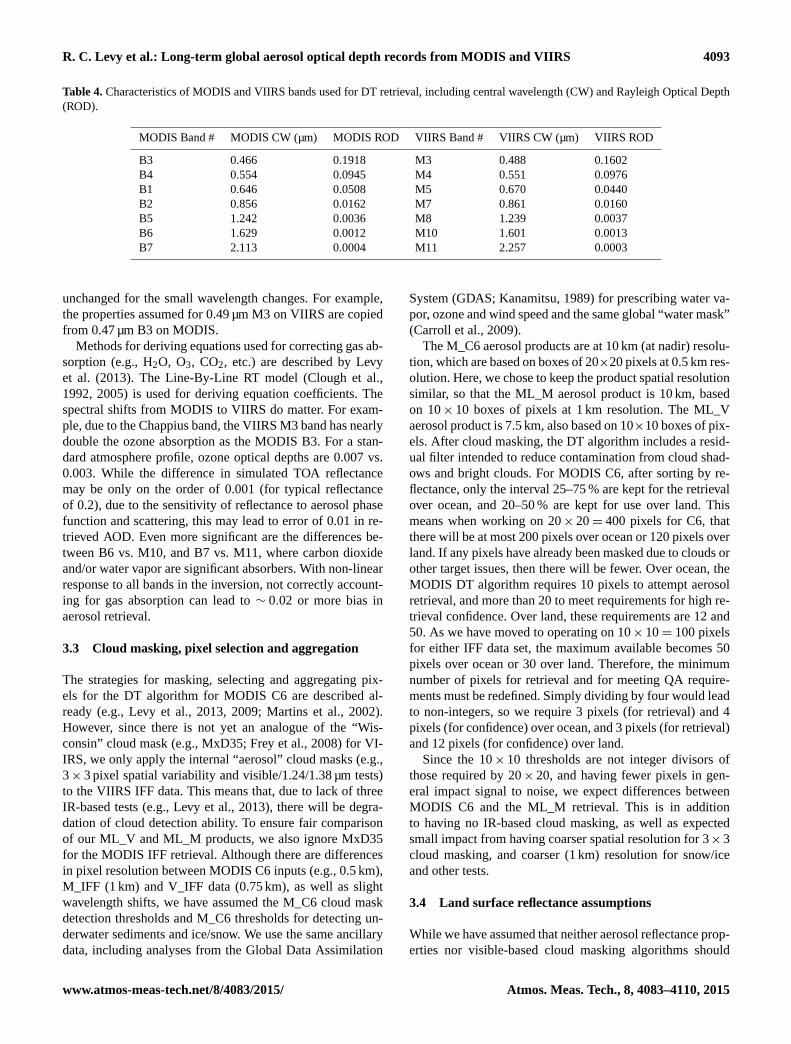
Table 4. Characteristics of MODIS and VIIRS bands used for DT retrieval, including central wavelength (CW) and Rayleigh Optical Depth
(ROD).
MODIS Band # MODIS CW (µm) MODIS ROD VIIRS Band # VIIRS CW (µm) VIIRS ROD
B3 0.466 0.1918 M3 0.488 0.1602
B4 0.554 0.0945 M4 0.551 0.0976
B1 0.646 0.0508 M5 0.670 0.0440
B2 0.856 0.0162 M7 0.861 0.0160
B5 1.242 0.0036 M8 1.239 0.0037
B6 1.629 0.0012 M10 1.601 0.0013
B7 2.113 0.0004 M11 2.257 0.0003
unchanged for the small wavelength changes. For example,
the properties assumed for 0.49 µm M3 on VIIRS are copied
from 0.47 µm B3 on MODIS.
Methods for deriving equations used for correcting gas ab-
sorption (e.g., H2O, O3, CO2, etc.) are described by Levy
et al. (2013). The Line-By-Line RT model (Clough et al.,
1992, 2005) is used for deriving equation coefficients. The
spectral shifts from MODIS to VIIRS do matter. For exam-
ple, due to the Chappius band, the VIIRS M3 band has nearly
double the ozone absorption as the MODIS B3. For a stan-
dard atmosphere profile, ozone optical depths are 0.007 vs.
0.003. While the difference in simulated TOA reflectance
may be only on the order of 0.001 (for typical reflectance
of 0.2), due to the sensitivity of reflectance to aerosol phase
function and scattering, this may lead to error of 0.01 in re-
trieved AOD. Even more significant are the differences be-
tween B6 vs. M10, and B7 vs. M11, where carbon dioxide
and/or water vapor are significant absorbers. With non-linear
response to all bands in the inversion, not correctly account-
ing for gas absorption can lead to ∼ 0.02 or more bias in
aerosol retrieval.
3.3 Cloud masking, pixel selection and aggregation
The strategies for masking, selecting and aggregating pix-
els for the DT algorithm for MODIS C6 are described al-
ready (e.g., Levy et al., 2013, 2009; Martins et al., 2002).
However, since there is not yet an analogue of the “Wis-
consin” cloud mask (e.g., MxD35; Frey et al., 2008) for VI-
IRS, we only apply the internal “aerosol” cloud masks (e.g.,
3× 3 pixel spatial variability and visible/1.24/1.38 µm tests)
to the VIIRS IFF data. This means that, due to lack of three
IR-based tests (e.g., Levy et al., 2013), there will be degra-
dation of cloud detection ability. To ensure fair comparison
of our ML_V and ML_M products, we also ignore MxD35
for the MODIS IFF retrieval. Although there are differences
in pixel resolution between MODIS C6 inputs (e.g., 0.5 km),
M_IFF (1 km) and V_IFF data (0.75 km), as well as slight
wavelength shifts, we have assumed the M_C6 cloud mask
detection thresholds and M_C6 thresholds for detecting un-
derwater sediments and ice/snow. We use the same ancillary
data, including analyses from the Global Data Assimilation
System (GDAS; Kanamitsu, 1989) for prescribing water va-
por, ozone and wind speed and the same global “water mask”
(Carroll et al., 2009).
The M_C6 aerosol products are at 10 km (at nadir) resolu-
tion, which are based on boxes of 20×20 pixels at 0.5 km res-
olution. Here, we chose to keep the product spatial resolution
similar, so that the ML_M aerosol product is 10 km, based
on 10× 10 boxes of pixels at 1 km resolution. The ML_V
aerosol product is 7.5 km, also based on 10×10 boxes of pix-
els. After cloud masking, the DT algorithm includes a resid-
ual filter intended to reduce contamination from cloud shad-
ows and bright clouds. For MODIS C6, after sorting by re-
flectance, only the interval 25–75 % are kept for the retrieval
over ocean, and 20–50 % are kept for use over land. This
means when working on 20× 20= 400 pixels for C6, that
there will be at most 200 pixels over ocean or 120 pixels over
land. If any pixels have already been masked due to clouds or
other target issues, then there will be fewer. Over ocean, the
MODIS DT algorithm requires 10 pixels to attempt aerosol
retrieval, and more than 20 to meet requirements for high re-
trieval confidence. Over land, these requirements are 12 and
50. As we have moved to operating on 10× 10= 100 pixels
for either IFF data set, the maximum available becomes 50
pixels over ocean or 30 over land. Therefore, the minimum
number of pixels for retrieval and for meeting QA require-
ments must be redefined. Simply dividing by four would lead
to non-integers, so we require 3 pixels (for retrieval) and 4
pixels (for confidence) over ocean, and 3 pixels (for retrieval)
and 12 pixels (for confidence) over land.
Since the 10× 10 thresholds are not integer divisors of
those required by 20× 20, and having fewer pixels in gen-
eral impact signal to noise, we expect differences between
MODIS C6 and the ML_M retrieval. This is in addition
to having no IR-based cloud masking, as well as expected
small impact from having coarser spatial resolution for 3×3
cloud masking, and coarser (1 km) resolution for snow/ice
and other tests.
3.4 Land surface reflectance assumptions
While we have assumed that neither aerosol reflectance prop-
erties nor visible-based cloud masking algorithms should
www.atmos-meas-tech.net/8/4083/2015/ Atmos. Meas. Tech., 8, 4083–4110, 2015

4094 R. C. Levy et al.: Long-term global aerosol optical depth records from MODIS and VIIRS
change much with respect to small spectral shifts (MODIS
vs. VIIRS), we cannot assume the same is true for assump-
tions of land surface optical properties (e.g., Fig. 4). For
MODIS, Levy et al. (2007b) derived band-to-band relation-
ships for surface reflectance, each described by a combina-
tion of ratios (slopes) and corrections (offsets). Specifically,
the nominal slopes were set at 0.53 and 0.49, for B3/B7 and
B1/B3, respectively, but were functions of scattering angle
and NDVI_SWIR (shortwave Normalized Difference Vege-
tation Index – a measure of surface “greenness”). The values
were considered “global”, so they would be representative
of many vegetated surfaces, and would minimize systematic
bias in retrieved AOD. However, the standard deviation of
the band ratios was large.
Under typical reflectance spectra for green vegetation,
Fig. 5 shows that surface properties within VIIRS bands are
different from those in MODIS bands. For the blue band,
reflectance is larger in VIIRS M3 (0.49 µm) as compared
MODIS B3 (0.47 µm), and yet in the red band, reflectance
is smaller in VIIRS M5 (0.67 µm) as compared to MODIS
B1 (0.65 µm). Clearly, surface reflectance ratios assumed for
MODIS will not work for VIIRS. Although the V_EDR
uses VIIRS-specific ratios derived from VIIRS-measured ra-
diances (Jackson et al., 2013), Liu et al. (2014) showed
that the ratio’s characterization could benefit from additional
(MODIS-like) information of surface greenness and scatter-
ing angle. Since, a complete MODIS-like surface reflectance
relationship requires a comprehensive atmospheric correc-
tion (e.g., Levy et al., 2007a) that has not been performed
yet, we have assumed the ratios used for the V_EDR without
benefit of any angle or greenness dependency. Specifically,
we assume ratios of 0.56 for M5/M11 and 0.65 for M3/M5
(Jackson et al., 2013). Thus, for this version of IFF retrieval,
we may see biases over some regions.
4 Results
Here we compare the MODIS-like products on MODIS and
VIIRS, with each other and with the standard MODIS C6 and
VIIRS_EDR products.
4.1 AOD: granule and daily imagery
Figure 6 shows the granule (5 March 2013 at 07:35 UTC) re-
trievals from ML_M and ML_V, comparable with the M_C6
and V_EDR imagery presented in Fig. 2. The MODIS-like
QA requirement is QAC= 3 over land and QAC≥ 1 over
ocean. As intended, the ML_V is more similar to the ML_M
(and thus to M_C6) than the V_EDR was to M_C6. Over
land, where both retrieve, the AOD values are closer, includ-
ing the region over Bangladesh identified in Fig. 2 where
M_C6 and V_EDR AOD differed by ∼ 0.3. However, there
is still some discrepancy in coverage, especially over eastern
India, which is retrieved as near-zero AOD by ML_M, but
still not retrieved by ML_V. It appears that the issue is iden-
tification of “bright” scenes not suitable for retrieval. The
retrieval is set up to degrade results (to lower QAC values)
when the observed reflectance in SWIR channel (2.11 for
MODIS, 2.26 µm for VIIRS) is greater than 0.25. Due to the
differences in this wavelength band, the decision to use or
not to use a particular ground location may vary between re-
trievals.
Figure 7a and b plots the MODIS-like retrievals (ML_V
and ML_M) for 29 May 2013 (RGB in Fig. 1). This date was
chosen for significant overlap of MODIS and VIIRS orbits
along with aerosol hotspots that could be visually compared.
Data are gridded to 1◦× 1◦ boxes (similar to MODIS Level
3), and filtered by QAC values. Clearly, VIIRS has greater
coverage than MODIS, so Fig. 7c shows aggregation for
when limiting VIIRS retrieval to a MODIS-like swath width
(constraining to sensor zenith angle < 60◦).
4.2 AOD: Level 2 retrieval statistics
We applied the ML algorithm to both MODIS and VIIRS-
IFF, for the entire Spring (MAM) 2013 season. Table 5
presents some statistics for the resulting along-orbit (Level
2) data, separately over ocean and land. When we consider
the number of possible retrievals (daytime for a particular
surface), the “non-filtered retrieval fraction” indicates how
many are populated with valid AOD (dark, cloud-free, non-
glint, etc), while the “QA-filtered retrieval fraction” repre-
sents the subset having higher confidence. Let us denote the
QA-filtered retrieval fraction as the “retrieval fraction”, or
“retrievability”, which depends on pixel resolution (Remer
et al., 2012), masking algorithms (cloud, surface, ice/snow,
etc.), and QA assignment (e.g., Levy et al., 2013). A consis-
tent algorithm would be expected to make similar choices,
so that under the same observing conditions, there would be
similar retrieval fraction. We will discuss retrievability fur-
ther in Sect. 4.4.
The last two columns in Table 5 report two different cal-
culations of mean global AOD. The first of these is the sim-
ple average of all QA-filtered pixels, and can be thought of
representing the sampling of the instrument, convolved with
choices of the retrieval algorithm. This “pixel-weighted”
view of the world is by definition, clear-sky biased (Levy
et al., 2009). The latter is computed by first creating a Level
3-like product (e.g., Fig. 3) and then taking the simple aver-
age of all grid values (no weighting by surface area). Thus,
observed differences in L3 global means convolve differ-
ences in retrieved L2 AOD with the sensor sampling and
algorithm retrievability. Interestingly, differences between
MODIS and VIIRS may be more or less (and of different
sign) whether considering the Level 2 or Level 3 aggrega-
tions (Levy et al., 2009). We will discuss global mean AOD
further in Sect. 4.3.
Over-ocean, the global QA-filtered mean AOD from the
ML_M algorithm (= 0.11) is similar to M_C6. With the
Atmos. Meas. Tech., 8, 4083–4110, 2015 www.atmos-meas-tech.net/8/4083/2015/

R. C. Levy et al.: Long-term global aerosol optical depth records from MODIS and VIIRS 4095
Figure 6. QA-filtered AOD at 0.55 µm over the Bay of Bengal on 5 March 2013 at 07:35, retrieved with MODIS-like algorithm on (a) MODIS
(at 10 km) and (b) VIIRS (at 7.5 km). This is the same observational overlap as pictured in Fig. 2.
Figure 7. AOD at 0.55 µm, retrieved using MODIS-like algorithm on MODIS (a) and VIIRS (b), created from all orbits during 29 May 2013
(see Fig. 1). (c) approximates the MODIS coverage by reducing the VIIRS swath to sensor view angles less than 60◦.
ML_V data set, it jumps by 0.02 or nearly 20 %, even for
the MODIS-width-like swath. The V_EDR value is 0.12.
Figure 8 compares relative histograms (normalized to the
total QA-filtered retrievals) of the QA-filtered AOD. Over
ocean (top), the overall histograms are similar, but the ML_V
and ML_V60 histograms are shifted slightly towards higher
AOD, suggesting that the difference in the ML_M and ML_V
AOD retrievals are due to a slight increase for every L2
pixel’s value rather than adding a few high values. The most
significant difference may be that the V_EDR does not pro-
vide data in the smallest bin (between −0.05 and 0.00),
whereas the MODIS algorithm allows for high quality re-
trievals of exactly zero (Levy et al., 2013).
Over land, all MODIS or MODIS-like products estimate
a global (Level 2) mean around 0.17, differing by less than
0.01. These are all less than the V_EDR mean of 0.20. The
histograms for land (Fig. 8b) retrievals show a very simi-
lar distribution for ML_M and ML_V, with large differences
compared to the V_EDR. The MODIS DT algorithms allow
retrievals of zero and small negative AOD (to −0.05) where
the V_EDR algorithm does not (see Fig. 8, bottom).
Whether over land or over ocean, reduced swath version
of ML_V (ML_V60) have generally the statistics as the full
swath versions. This means that the discrepancies between
ML_V and the MODIS retrievals are not due to the increased
VIIRS sampling.
4.3 AOD: seasonal maps and statistics
Figures 9 and 10 follow from Figs. 3 and 4, showing sea-
sonal (MAM, Spring 2013) maps and scatterplots of 1◦× 1◦
AOD, for ML_M and ML_V data sets. Global means (equal
weighting for each grid cell) are reported as the last column
in Table 5.
Based on simple averaging of the 1◦×1◦ grids, the global
mean for ML_M is within 0.01 of M_C6. Figure 9d plots
the difference between ML_M (Fig. 9a) and M_C6 (Fig. 3a)
www.atmos-meas-tech.net/8/4083/2015/ Atmos. Meas. Tech., 8, 4083–4110, 2015

4096 R. C. Levy et al.: Long-term global aerosol optical depth records from MODIS and VIIRS
Table 5. Spring 2013 (March–April–May) statistics of QA-filtered AOD, retrieved over ocean (top) and land (bottom). QA-filtering for the
MODIS and MODIS-like products is QAC≥ 1 over ocean and QAC= 3 over land, whereas for the VIIRS EDR it is QAC= 3 only for both
surfaces.
Product Land or AOD Non-filtered QA-filtered Number of Mean AOD Mean AOD
Ocean resolution retrieval retrieval QA-filtered (pixel (equal
(km) fraction fraction retrievals weighted) 1◦× 1◦)
M_C6 Ocean 10 0.187 0.183 4.24×10⁷ 0.115 0.127
ML_M Ocean 10 0.146 0.145 3.34×10⁷ 0.113 0.122
ML_V Ocean 7.5 0.176 0.173 1.25×10⁸ 0.134 0.148
ML_V60 Ocean 7.5 0.171 0.169 1.07×10⁸ 0.132 0.144
V_EDR Ocean 6 0.352 0.123 1.41×10⁸ 0.122 0.130
M_C6 Land 10 0.140 0.069 6.63×10⁶ 0.175 0.146
ML_M Land 10 0.133 0.074 6.97×10⁶ 0.168 0.154
ML_V Land 7.5 0.132 0.074 1.97×10⁷ 0.169 0.160
ML_V60 Land 7.5 0.132 0.074 1.71×10⁷ 0.170 0.158
V_EDR Land 6 0.289 0.075 3.33×10⁷ 0.199 0.217
maps, showing that most grids also have differences (of less
than 0.01). However, it is interesting that global AOD is re-
duced over ocean (from 0.127 to 0.122), but is increased over
land (from 0.146 to 0.154). Even more interesting is that the
ML_M–M_C6 differences vary whether using gridded data,
as compared to using along orbit (L2) data. In fact, they are
of opposite sign depending on surface. Whereas the global
over-ocean AOD reduced under either averaging protocol,
the global over-land AOD is increased under gridded aver-
aging, but decreased under L2 averaging. Clearly, there is
a complex interplay between the concepts of aggregating and
averaging, between clear-sky bias (e.g., Levy et al., 2013)
and retrievability (e.g., Remer et al., 2012).
Figure 9d shows that whether over ocean or land, the
biggest per-grid differences are along the mid-latitude storm
belts, mostly driven by differences in cloud masking. These
arise from the combination of coarser pixel resolution (1 vs.
0.5 km) and lack of thermal infrared-based (e.g., MxD35)
cloud mask information, together causing systematic bias in
pixel selection and aggregation for retrieval (e.g., Martins
et al., 2002). Over ocean, although this makes little or no
difference for most grid cells (e.g., Fig. 10a), there are some
grid cells with much larger differences (tending toward re-
duced AOD). The result is that R2= 0.884 is less than unity
and that gridded data tends to show larger differences be-
tween ML_V and M_C6 than does along-orbit (Level 2) re-
trievals. By substituting the full MxD35 cloud mask (from
M_C6) into the ML_M retrieval (not shown explicitly here),
we confirmed that the cloud mask is the major culprit.
Over land, while reduced-resolution cloud masking con-
tributes to the discrepancies between ML_M and M_C6, the
more pertinent issue is the resolution’s impact on surface fea-
ture masking. The coarser resolution impacts ice/snow mask-
ing, in that sub-pixel snow can elude a coarse (1 km) resolu-
tion snow mask. This will tend to lead to higher-retrieved
AOD. Similarly, sub-pixel inland water (and coastlines) can
elude a coarser-resolution inland water mask, leading to
lower-retrieved AOD. Although we do not describe every
grid and how it contributes to global mean, it is clear that
both resolution and upstream information do matter. Interest-
ingly, however, even with an overall high bias, the R-squared
for land grids is extremely high (R2= 0.969; Fig. 10b).
We now move from the ML_M to the ML_V, for which
presumably, the differences in upstream information (no
Wisconsin cloud mask or thermal IR, and more similar res-
olutions) should be less important. Figure 9e plots the dif-
ference between the ML_V and ML_M maps, and Fig. 10c
and d compare ML_V with ML_M for collocated grids over
ocean and land.
Certainly, the bias pattern for ML_V compared to ML_M
is significantly different than for the V_EDR compared to
the M_C6 (even accounting for the small ML_M vs. M_C6
biases). Since Fig. 9f shows that there is essentially no dif-
ference between the reduced swath (Fig. 9c) and the entire
swath (Fig. 9b), we cannot blame the bias pattern of Fig. 9e
on VIIRS having a wider swath with more oblique viewing
angles. At least for this particular season, the differences in
sampling (e.g., Colarco et al., 2014) do not influence the grid-
ded or global means.
Thus, over ocean (Figs. 9e and 10c), the use of the ML
algorithm on VIIRS has introduced a bias as compared to
MODIS, which was not observed in the original compari-
son between the V_EDR and M_C6. The R-squared between
ML_V and ML_M for collocated grids is only slightly lower
(R2= 0.86), but the bias is significantly greater (B = 0.025)
than was seen for the V_EDR. We do note, however, that part
of this reduction in correlation has come from the 13 % in-
crease in the number of collocations (from 32 476 to 36 742),
primarily found over the far southern and northern oceans.
These regions are difficult to retrieve (e.g., Shi et al., 2011),
Atmos. Meas. Tech., 8, 4083–4110, 2015 www.atmos-meas-tech.net/8/4083/2015/

R. C. Levy et al.: Long-term global aerosol optical depth records from MODIS and VIIRS 4097
Ocean
0.0
0.1
0.2
0.3
0.4
Nor
mal
ized
Fre
quen
cy
−0.05 0.0
00.0
10.0
30.0
50.1
00.1
50.2
00.2
50.3
00.4
00.5
00.7
01.0
01.5
02.0
03.0
05.0
0
AOD Bins (0.55 µm)
M_C6ML_MML_V
ML_V, VZA < 60V_EDR
Land
0.00
0.05
0.10
0.15
0.20
0.25
Nor
mal
ized
Fre
quen
cy
−0.05 0.0
00.0
10.0
30.0
50.1
00.1
50.2
00.2
50.3
00.4
00.5
00.7
01.0
01.5
02.0
03.0
05.0
0
AOD Bins (0.55 µm)
A
B
Figure 8. Spring 2013 (March–April–May) relative frequency his-
tograms of QA-filtered AOD, retrieved over ocean (top) and land
(bottom). Note the non-uniform bin width, and that negative values
are allowed in the MODIS C6 and MODIS-like data sets over land.
See Table 5 for the number of QA-filtered pixels in each data set.
and correlation improves if they are not included in the scat-
terplot. However, Fig. 9e shows that the bias is present over
all of the global oceans, and remains even if the far northern
and southern oceans are excluded.
On the other hand, the ML_V retrieval over land, (Figs. 9e
and 10d), unequivocally reduces regional biases by an or-
der of magnitude as compared to V_EDR, and the global
mean is much closer to either ML_M or M_C6. The R-
squared for ML_M and ML_V collocated grids is impressive
(R2= 0.935) with negligible (0.006) bias.
From the combination of Figs. 9 and 10, it is clear that
ML_V provides a different view of the world than the
V_EDR. The ML_V world looks much more like MODIS’s
over land, but it has a 20 % high bias over ocean.
4.4 AOD: retrievability
As a function of geography, geometry and the state of the
atmosphere, can we quantify the chance that a particular al-
gorithm will derive a high-confidence value for AOD? In
terms of where and when seasonal mean AOD are derived,
we focus on the concept of retrievability, in order to evalu-
ate whether the algorithms have made similar choices under
similar conditions.
Table 5 shows general agreement for the non-filtered re-
trieval fraction between all versions of the MODIS-like al-
gorithm, ranging between 0.146 and 0.187 over ocean and
0.132 and 0.140 over land. In other words, approximately
15–19 % of all 10 km (or 7.5) km boxes are retrieved over
land, with 13 % over ocean. This value is much less than
the V_EDR, which reports an AOD value in 35.2 % of
all retrieval boxes over ocean and 28.9 % over land. How-
ever, when it comes to assigning confidence to the retrieval,
the resulting retrieval fraction converges somewhat. Over
ocean, nearly 99 % of the retrieved values meet QAC thresh-
olds under MODIS-like logic, but only a third meet the
stricter V_EDR requirements. Therefore, after QA-filtering,
the retrieval fraction for the V_EDR actually becomes lower
(0.123) than any MODIS or MODIS-like retrieval (≥ 0.145).
There is negligible difference between the full ML_V and
(the reduced swath of) the ML_V60. Over land, after QAC
filtering, all algorithms retrieve about 7 %.
For this section, let us use the ML_M as a baseline. Fig-
ure 11 shows that although over-ocean retrieval fraction aver-
ages near 15 % and over-land near 7 %, the retrieval fraction
differs greatly by region. As expected, sparse or no retrieval
is made over the deserts and snow surfaces. Yet, interest-
ingly, the largest retrieval fractions are adjacent to deserts,
including pre-monsoon India (Thar), southern Africa (Kala-
hari) and the Sahel (Sahara). These regions have low rainfall
and cloud cover during MAM 2013. Over ocean, while the
retrieval fraction is more balanced, there tends to be lower
retrieval fraction over cloudy areas (ITCZ and midlatitude
storm tracks).
Figure 12 plots global retrieval fraction from the three
other algorithms as compared to ML_M (Fig. 11). The top
row shows difference maps, while the middle and bottom
rows are scatterplots comparing the 1◦ grids, for ocean and
land, respectively. Left, middle and right columns show
M_C6, ML_V and V_EDR as compared to ML_M.
Among the MODIS-like products, Table 5 showed that
the largest global retrievability difference was between the
M_C6 (0.18) and ML_M (0.14) over ocean. Examining
Fig. 12a and d, this retrievability difference is nearly every-
where, in that all original M_C6 data had ∼ 0.04 greater re-
trieval fraction than ML_M. However, looking closer, we see
that there are two regimes contrary to the high bias. Close
to coastlines (e.g., the west coasts of North America and
Africa), there is not a large difference between the two data
sets. These are the grids that make up the arm that nearly
www.atmos-meas-tech.net/8/4083/2015/ Atmos. Meas. Tech., 8, 4083–4110, 2015
4098 R. C. Levy et al.: Long-term global aerosol optical depth records from MODIS and VIIRS
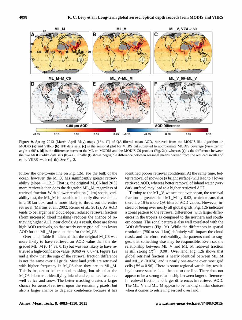
Figure 9. Spring 2013 (March–April–May) maps (1◦× 1◦) of QA-filtered mean AOD, retrieved from the MODIS-like algorithm on
MODIS (a) and VIIRS (b) IFF data sets. (c) is the seasonal plot for VIIRS but subsetted to approximate MODIS coverage (view zenith
angle< 60◦). (d) is the difference between the ML on MODIS and the MODIS C6 product (Fig. 2a), whereas (e) is the difference between
the two MODIS-like data sets (b)–(a). Finally (f) shows negligible difference between seasonal means derived from the reduced swath and
entire VIIRS swath (c)–(b). See Fig. 2.
follow the one-to-one line on Fig. 12d. For the bulk of the
ocean, however, the M_C6 has significantly greater retriev-
ability (slope = 1.21). That is, the original M_C6 had 20 %
more retrievals than does the degraded ML_M, regardless of
retrieval fraction. With a lower resolution (1 km) spatial vari-
ability test, the ML_M is less able to identify discrete clouds
in a 10 km box, and is more likely to throw out the entire
retrieval (Martins et al., 2002; Remer et al., 2012). As AOD
tends to be larger near cloud edges, reduced retrieval fraction
(from increased cloud masking) reduces the chance of re-
trieving higher AOD near clouds. As a result, there are fewer
high AOD retrievals, so that nearly every grid cell has lower
AOD for the ML_M product than for the M_C6.
Over land, Table 5 indicated that the original M_C6 was
more likely to have retrieved an AOD value than the de-
graded ML_M (0.14 vs. 0.13) but was less likely to have re-
trieved a high-confidence value (0.069 vs. 0.074). Figure 12a
and g show that the sign of the retrieval fraction difference
is not the same over all grids. Most land grids are retrieved
with higher frequency in M_C6 than they are in ML_M.
This is in part to better cloud masking, but also that the
M_C6 is better at identifying inland and ephemeral water as
well as ice and snow. The better masking creates a larger
chance for aerosol retrieval upon the remaining pixels, but
also a larger chance to degrade confidence because it has
identified poorer retrieval conditions. At the same time, bet-
ter removal of snow/ice (a bright surface) will lead to a lower
retrieved AOD, whereas better removal of inland water (very
dark surface) may lead to a higher retrieved AOD.
Turning to the ML_V, we see that over ocean, the retrieval
fraction is greater than ML_M by 0.03, which means that
there are 16 % more QA-filtered AOD values. However, in-
stead of being over nearly all global grids, Fig. 12b indicates
a zonal pattern to the retrieval differences, with larger differ-
ences in the tropics as compared to the northern and south-
ern oceans. The zonal pattern is also well correlated with the
AOD differences (Fig. 9e). While the differences in spatial
resolution (750 m vs. 1 km) definitely will impact the cloud
mask, and therefore retrievability, the patterns tend to sug-
gest that something else may be responsible. Even so, the
relationship between ML_V and ML_M retrieval fraction
is still strong (R2= 0.90). Over land, Fig. 12h shows that
global retrieval fraction is nearly identical between ML_M
and ML_V (0.074), and is nearly one-to-one over most grid
cells (R2= 0.96). There is some regional variability, result-
ing in some scatter about the one-to-one line. There does not
appear to be a strong relationship between larger differences
in retrieval fraction and larger differences in retrieved AOD.
The ML_V and ML_M appear to be making similar choices
when it comes to retrieving aerosol over land.
Atmos. Meas. Tech., 8, 4083–4110, 2015 www.atmos-meas-tech.net/8/4083/2015/
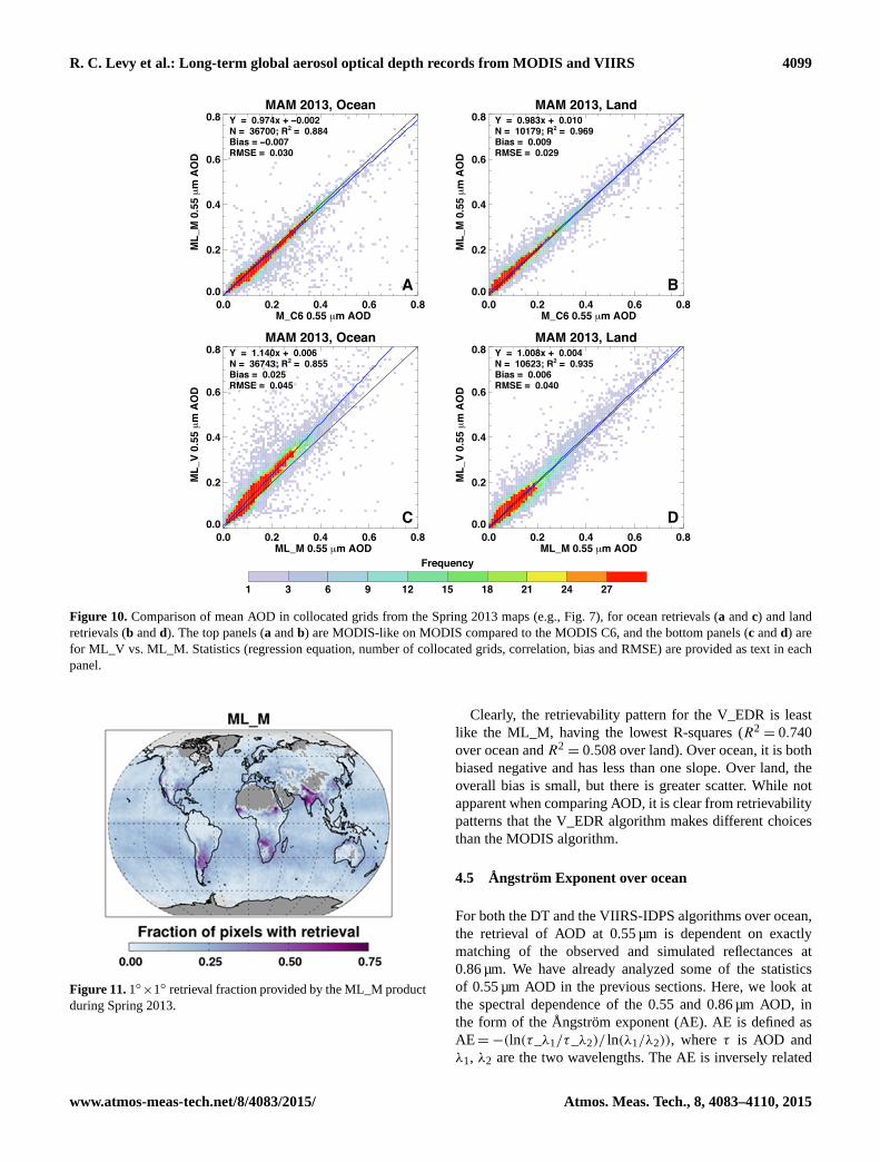
R. C. Levy et al.: Long-term global aerosol optical depth records from MODIS and VIIRS 4099
MAM 2013, Ocean
0.0 0.2 0.4 0.6 0.8M_C6 0.55 µm AOD
0.0
0.2
0.4
0.6
0.8
ML_
M 0
.55 µ
m A
OD
Y = 0.974x + −0.002N = 36700; R2 = 0.884Bias = −0.007RMSE = 0.030
A
MAM 2013, Land
0.0 0.2 0.4 0.6 0.8M_C6 0.55 µm AOD
0.0
0.2
0.4
0.6
0.8
ML_
M 0
.55 µ
m A
OD
Y = 0.983x + 0.010N = 10179; R2 = 0.969Bias = 0.009RMSE = 0.029
B
MAM 2013, Ocean
0.0 0.2 0.4 0.6 0.8ML_M 0.55 µm AOD
0.0
0.2
0.4
0.6
0.8
ML_
V 0.
55 µ
m A
OD
Y = 1.140x + 0.006N = 36743; R2 = 0.855Bias = 0.025RMSE = 0.045
C
MAM 2013, Land
0.0 0.2 0.4 0.6 0.8ML_M 0.55 µm AOD
0.0
0.2
0.4
0.6
0.8
ML_
V 0.
55 µ
m A
OD
Y = 1.008x + 0.004N = 10623; R2 = 0.935Bias = 0.006RMSE = 0.040
D
1 3 6 9 12 15 18 21 24 27
Frequency
Figure 10. Comparison of mean AOD in collocated grids from the Spring 2013 maps (e.g., Fig. 7), for ocean retrievals (a and c) and land
retrievals (b and d). The top panels (a and b) are MODIS-like on MODIS compared to the MODIS C6, and the bottom panels (c and d) are
for ML_V vs. ML_M. Statistics (regression equation, number of collocated grids, correlation, bias and RMSE) are provided as text in each
panel.
Figure 11. 1◦×1◦ retrieval fraction provided by the ML_M product
during Spring 2013.
Clearly, the retrievability pattern for the V_EDR is least
like the ML_M, having the lowest R-squares (R2= 0.740
over ocean and R2= 0.508 over land). Over ocean, it is both
biased negative and has less than one slope. Over land, the
overall bias is small, but there is greater scatter. While not
apparent when comparing AOD, it is clear from retrievability
patterns that the V_EDR algorithm makes different choices
than the MODIS algorithm.
4.5 Ångström Exponent over ocean
For both the DT and the VIIRS-IDPS algorithms over ocean,
the retrieval of AOD at 0.55 µm is dependent on exactly
matching of the observed and simulated reflectances at
0.86 µm. We have already analyzed some of the statistics
of 0.55 µm AOD in the previous sections. Here, we look at
the spectral dependence of the 0.55 and 0.86 µm AOD, in
the form of the Ångström exponent (AE). AE is defined as
AE=−(ln(τ_λ1/τ_λ2)/ ln(λ1/λ2)), where τ is AOD and
λ1, λ2 are the two wavelengths. The AE is inversely related
www.atmos-meas-tech.net/8/4083/2015/ Atmos. Meas. Tech., 8, 4083–4110, 2015

4100 R. C. Levy et al.: Long-term global aerosol optical depth records from MODIS and VIIRS
MAM 2013, Ocean
0.0 0.2 0.4 0.6 0.8ML_M Retrieval Fraction
0.0
0.2
0.4
0.6
0.8
M_C
6 Re
triev
al F
ract
ion Y = 1.208x + 0.011
N = 37708; R2 = 0.964Bias = 0.043RMSE = 0.050
MAM 2013, Ocean
0.0 0.2 0.4 0.6 0.8ML_M Retrieval Fraction
0.0
0.2
0.4
0.6
0.8M
L_V
Retri
eval
Fra
ctio
n Y = 1.163x + −0.004N = 37741; R2 = 0.901Bias = 0.030RMSE = 0.049
MAM 2013, Ocean
0.0 0.2 0.4 0.6 0.8ML_M Retrieval Fraction
0.0
0.2
0.4
0.6
0.8
V_ED
R Re
triev
al F
ract
ion Y = 1.088x + −0.038
N = 33280; R2 = 0.740Bias = −0.026RMSE = 0.062
MAM 2013, Land
0.0 0.2 0.4 0.6 0.8ML_M Retrieval Fraction
0.0
0.2
0.4
0.6
0.8
M_C
6 Re
triev
al F
ract
ion Y = 1.005x + −0.004
N = 11334; R2 = 0.976Bias = −0.005RMSE = 0.021
MAM 2013, Land
0.0 0.2 0.4 0.6 0.8ML_M Retrieval Fraction
0.0
0.2
0.4
0.6
0.8
ML_
V Re
triev
al F
ract
ion Y = 0.956x + 0.005
N = 11514; R2 = 0.963Bias = −0.000RMSE = 0.024
MAM 2013, Land
0.0 0.2 0.4 0.6 0.8ML_M Retrieval Fraction
0.0
0.2
0.4
0.6
0.8V_
EDR
Retri
eval
Fra
ctio
n Y = 0.723x + 0.031N = 11223; R2 = 0.508Bias = −0.007RMSE = 0.090
1 4 8 12 16 20 24 28 32 36
Frequency
D E F
G H I
A B C
Figure 12. Comparing retrieval fraction between each product and the ML_M product (Fig. 11). The top row (a–c) are difference maps,
whereas the bottom two rows (d–f for ocean and g–i for land) are frequency scatterplots.
to the general size of the aerosol particles, so that smaller val-
ues (AE< 1.0) are associated with large-sized (e.g., dust or
sea salt) and larger values (AE> 1.0) are indicative of com-
bustion (pollution or smoke) particles.
Figure 13 presents Spring (MAM) 2013 statistics for the
AE over ocean, computed for each of the different data sets.
Maps of AE are calculated by creating separate maps of AOD
at 0.55 µm (e.g., Figs. 3 and 9) and 0.86 µm, so that AE can
be calculated at each grid box from the means of these two
wavelengths. There are no filters for minimum AOD. For the
original MODIS C6 data (Fig. 13a), the Saharan dust belt
and the sea salt of the southern oceans are clearly marked
by AE< 0.5. The Asian pollution and US East Coast pollu-
tion plumes have AE> 1.0. The ML_M map (Fig. 13b) is
nearly identical, with R2= 0.935 and mean bias less than
0.01. Although the ML_V map is well correlated with the
ML_M (R2= 0.82 for collocated grids in Fig. 13g), and
spatial features are similar, its regression is not one-to-one
(slope= 0.81, offset= 0.24; bias= 0.12). The AE map of
the V_EDR, however, does not resemble MODIS or MODIS-
Atmos. Meas. Tech., 8, 4083–4110, 2015 www.atmos-meas-tech.net/8/4083/2015/
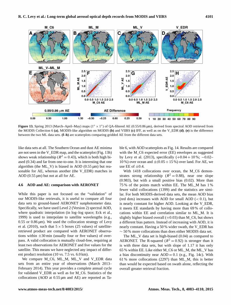
R. C. Levy et al.: Long-term global aerosol optical depth records from MODIS and VIIRS 4101
Figure 13. Spring 2013 (March–April–May) maps (1◦× 1◦) of QA-filtered AE (0.55/0.86 µm), derived from spectral AOD retrieved from
the MODIS Collection 6 (a), MODIS-like algorithm on MODIS (b) and VIIRS (c) IFF, as well as on the V_EDR (d). (e) is the difference
between the two ML data sets. (f–h) are scatterplots comparing gridded AE from the different data sets.
like data sets at all. The Southern Ocean and dust AE minima
are not seen in the V_EDR map, and the scatterplot (Fig. 13h)
shows weak relationship (R2= 0.43), which is both high bi-
ased (0.34) and far from one-to-one. It is interesting that one
algorithm (the ML_V) is biased in AOD (0.55 µm) but rea-
sonable for AE, whereas another (the V_EDR) matches in
AOD (0.55 µm) but not at all for AE.
4.6 AOD and AE: comparison with AERONET
While this paper is not focused on the “validation” of
our MODIS-like retrievals, it is useful to compare all four
data sets to ground-based AERONET sunphotometer data.
Specifically, we have used Level 2 (Version 2) spectral AOD,
where quadratic interpolation (in log–log space; Eck et al.,
1999) is used to interpolate to satellite wavelengths (e.g.,
0.55 or 0.86 µm). We used the collocation strategy of Levy
et al. (2010), such that 5× 5 boxes (25 values) of satellite-
retrieved product are compared with AERONET observa-
tions within ±30 min (usually four or five values) of over-
pass. A valid collocation is mutually cloud-free, requiring at
least two observations for AERONET and five values for the
satellite. This means we have neglected any impact of differ-
ent product resolution (10 vs. 7.5 vs. 6.0 km).
We compare M_C6, ML_M, ML_V and V_EDR data
sets from an entire year of observations (March 2013–
February 2014). This year provides a complete annual cycle
for validated V_EDR as well as for M_C6. Statistics of the
collocations (AOD at 0.55 µm and AE) are reported as Ta-
ble 6, with AOD scatterplots as Fig. 14. Results are compared
with the M_C6 expected error (EE) envelopes as suggested
by Levy et al. (2013), specifically (+0.04+ 10 %; −0.02–
10 %) over ocean and ±(0.05+15 %) over land. For AE, we
use EE of ±0.4.
With 1418 collocations over ocean, the M_C6 demon-
strates strong relationship (R2= 0.88), near one slope
(0.983), but with a small positive bias (0.02). More than
75 % of the points match within EE. The ML_M has 1 %
fewer valid collocations (1399) and the statistics are simi-
lar. For both MODIS-derived data sets, the mean AOD bias
(red dots) increases with AOD for small AOD (< 0.1), but
is nearly constant for higher AOD. Looking at the V_EDR,
it meets EE standards by having more than 69 % of collo-
cations within EE and correlation similar to ML_M. It is
slightly higher biased overall (+0.03) than M_C6, but shows
a different bias pattern. Instead of increasing with AOD, it is
nearly constant. Having a 50 % wider swath, the V_EDR has
∼ 50 % more collocations than does either MODIS data set.
The ML_V data set is high-biased (0.04) as compared to
AERONET. The R-squared (R2= 0.92) is stronger than it
is with three data sets, but with slope of 1.17 it has only
65 % within EE. Like either M_C6 or ML_M, the ML_V has
a bias discontinuity near AOD= 0.1 (e.g., Fig. 14c). With
61 % more collocations (2297) than ML_M, this is better
than would be expected based on swath alone, reflecting the
overall greater retrieval fraction.
www.atmos-meas-tech.net/8/4083/2015/ Atmos. Meas. Tech., 8, 4083–4110, 2015
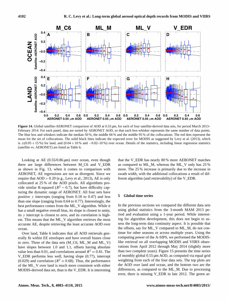
4102 R. C. Levy et al.: Long-term global aerosol optical depth records from MODIS and VIIRS
−0.4
−0.2
−0.0
0.2
0.4Sa
telli
te−A
ERO
NET
AOD
OCE
ANM_C6
AML_M
BML_V
CV_EDR
D
0.0 0.2 0.4 0.6AERONET 0.55 µm AOD
−0.4
−0.2
−0.0
0.2
0.4
Sate
llite−A
ERO
NET
AOD
LAND
E
0.0 0.2 0.4 0.6AERONET 0.55 µm AOD
F
0.0 0.2 0.4 0.6AERONET 0.55 µm AOD
G
0.0 0.2 0.4 0.6AERONET 0.55 µm AOD
H
Figure 14. Global satellite-AERONET comparison of AOD at 0.55 µm, for each of four satellite-derived data sets, for period March 2013–
February 2014. For each panel, data are sorted by AERONET AOD, so that each box-whisker represents the same number of data points.
The blue box and whiskers indicate the median 50 %, the middle 66 % and the middle 95 % of the collocations. The red dots represent the
mean for the set of collocations. The solid black lines indicate the expected error for MODIS as suggested by Levy et al. (2013), which
is ±(0.05+ 15 %) for land, and (0.04+ 10 % and −0.02–10 %) over ocean. Details of the statistics, including linear regression statistics
(satellite vs. AERONET) are listed as Table 6.
Looking at AE (0.55/0.86 µm) over ocean, even though
there are large differences between M_C6 and V_EDR
as shown in Fig. 13, when it comes to comparison with
AERONET, AE regressions are not as divergent. Since we
require that AOD> 0.20 (e.g., Levy et al., 2013), AE is only
collocated at 25 % of the AOD pixels. All algorithms pro-
vide similar R-squared (R2∼ 0.7), but have difficulty cap-
turing the dynamic range of AERONET. All four sets have
positive y intercepts (ranging from 0.18 to 0.47) and less
than one slope (ranging from 0.64 to 0.77). Interestingly, the
best performance comes from the ML_V algorithm. While it
has a small negative overall bias, its slope is closest to unity,
its y intercept is closest to zero, and its correlation is high-
est. This means that the ML_V algorithm retrieves the most
accurate AE, despite retrieving the least accurate AOD over
ocean.
Over land, Table 6 indicates that all AOD retrievals gen-
erally fit within EE envelopes and have overall biases close
to zero. Three of the data sets (M_C6, ML_M and ML_V)
have slopes between 1.0 and 1.1, offsets having absolute
value less than 0.01, and correlations around R2= 0.81. The
V_EDR performs less well, having slope (0.77), intercept
(0.029) and correlation (R2= 0.68). Thus, the performance
of the ML_V over land is much more consistent with either
MODIS-derived data set, than is the V_EDR. It is interesting
that the V_EDR has nearly 80 % more AERONET matches
as compared to ML_M, whereas the ML_V only has 25 %
more. The 25 % increase is primarily due to the increase in
swath width, with the additional collocations a result of dif-
ferent algorithm (and retrievability) of the V_EDR.
5 Global time series
In the previous sections we compared the different data sets
using global statistics from the 3-month MAM 2013 pe-
riod and evaluation using a 1-year period. While interest-
ing for algorithm development, this does not begin to as-
sess the long-term data continuity aspect. It is possible that
the offsets, say for ML_V compared to ML_M, do not con-
tinue for other seasons or across multiple years. Using the
computing power of the A-SIPS, we performed the MODIS-
like retrieval on all overlapping MODIS and VIIRS obser-
vations from April 2012 through May 2014 (slightly more
than two complete years). Figure 15 presents the time series
of monthly global 0.55 µm AOD, as computed via equal grid
weighting from each of the four data sets. The top plots are
the AOD over land and ocean, and the bottom two are the
differences, as compared to the ML_M. Due to processing
error, there is missing V_EDR in late 2012. The green ar-
Atmos. Meas. Tech., 8, 4083–4110, 2015 www.atmos-meas-tech.net/8/4083/2015/
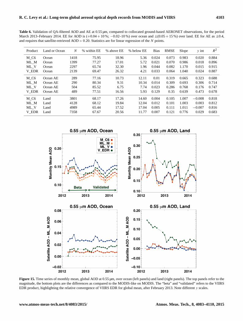
R. C. Levy et al.: Long-term global aerosol optical depth records from MODIS and VIIRS 4103
Table 6. Validation of QA-filtered AOD and AE at 0.55 µm, compared to collocated ground-based AERONET observations, for the period
March 2013–February 2014. EE for AOD is (+0.04+ 10 %; −0.02–10 %) over ocean and ±(0.05+ 15 %) over land. EE for AE as ±0.4,
and requires that satellite-retrieved AOD> 0.20. Statistics are for linear regression of the N points.
Product Land or Ocean N % within EE % above EE % below EE Bias RMSE Slope y int R2
M_C6 Ocean 1418 75.95 18.96 5.36 0.024 0.073 0.983 0.020 0.884
ML_M Ocean 1399 77.27 17.01 5.72 0.021 0.070 0.986 0.018 0.896
ML_V Ocean 2297 65.74 32.30 1.96 0.044 0.082 1.170 0.015 0.915
V_EDR Ocean 2139 69.47 26.32 4.21 0.033 0.064 1.040 0.024 0.887
M_C6 Ocean AE 289 77.16 10.73 12.11 0.01 0.319 0.665 0.323 0.688
ML_M Ocean AE 290 80.34 9.31 10.34 0.014 0.309 0.693 0.306 0.714
ML_V Ocean AE 504 85.52 6.75 7.74 0.023 0.286 0.768 0.176 0.747
V_EDR Ocean AE 489 77.51 16.56 5.93 0.129 0.35 0.639 0.473 0.678
M_C6 Land 3801 68.17 17.26 14.60 0.004 0.105 1.007 −0.008 0.818
ML_M Land 4128 68.12 19.84 12.04 0.012 0.101 1.003 0.003 0.812
ML_V Land 4989 65.44 17.52 17.04 0.005 0.111 1.011 −0.007 0.816
V_EDR Land 7358 67.67 20.56 11.77 0.007 0.121 0.776 0.029 0.683
Figure 15. Time series of monthly mean, global AOD at 0.55 µm, over ocean (left panels) and land (right panels). The top panels refer to the
magnitude, the bottom plots are the differences as compared to the MODIS-like on MODIS. The “beta” and “validated” refers to the VIIRS
EDR product, highlighting the relative convergence of VIIRS EDR for global mean, after February 2013. Note different y scales.
www.atmos-meas-tech.net/8/4083/2015/ Atmos. Meas. Tech., 8, 4083–4110, 2015

4104 R. C. Levy et al.: Long-term global aerosol optical depth records from MODIS and VIIRS
rows on Fig. 15a denote the relative periods of “beta” quality
and “validated stage 2” quality V_EDR data.
Over ocean, all time series show the same seasonal cycle
(Fig. 15a). Highest AOD is observed during the May/June
months, with lowest during the October/November months.
An average ∼ 0.008 offset between M_C6 and ML_M is ap-
parent for all months, with little variability over time. An av-
erage ∼ 0.012 offset between V_EDR and ML_M is appar-
ent, but it apparently increases over time. In fact, the offset
after February 2013 continues to increase, approaching 0.02
by 2014. The pattern of the ML_V compared to ML_M is
interesting. While the ∼ 0.025 offset does not change from
year to year, the offset is even larger (more than 0.035) during
the late spring maximums. This represents the combination
of extra retrieval fraction and enhanced AOD observed dur-
ing the late spring aerosol transports (from Asia and Africa).
Over land, there is also a seasonal cycle observed
(Fig. 15b) by both ML_M and M_C6, but there are two
humps (Northern Hemisphere early winter and late spring),
along with much more variability. There are minima in Oc-
tober of both years, with 2013 lower than 2012. Although
we saw nearly identical AOD for the MAM 2013 period (Ta-
ble 5), the offset between ML_M and M_C6 actually varies
with season, ranging from near zero to as large as 0.02 dur-
ing the late spring and through the summers. Interestingly,
the variability of ML_V compared to ML_M is less than
M_C6 compared to ML_M. Finally, while the V_EDR set-
tles down towards the ML_M after February 2013 (validated
stage 2), the monthly offsets remain large (∼ 0.03) and vari-
able (±0.02).
6 Discussion
In the previous sections, we first compared the V_EDR data
product with M_C6. Then, we created a simplified MODIS-
like algorithm that was run on the MODIS-IFF data (ML_M)
and VIIRS-IFF data (ML_V). Based on the figures and statis-
tics, we saw the following.
– The 0.55 µm AOD from V_EDR over ocean is similar
to M_C6. Global mean AOD is within ±0.01 of M_C6.
While V_EDR has significantly more coverage, over-
all retrieval fraction is smaller. For common 1◦× 1◦
grids, AOD relationship is strong (R2= 0.89) and re-
gression is near one-to-one. Compared to AERONET,
the V_EDR and M_C6 both meet expected error re-
quirements. The V_EDR has fewer retrievals of small
AOD< 0.02.
– Over-ocean AE (0.55/0.86 µm) retrieved from V_EDR
is offset high and has weak relationship to M_C6 (R2=
0.43).
– Over land, the V_EDR has positive offset and provides
different spatial coverage of AOD. The V_EDR does
not retrieve negative AOD. R2 < 0.58, slope is 0.68 and
offset is 0.10. AERONET collocation confirms that the
V_EDR is too high at low AOD and too low at high
AOD.
– Primarily due to cloud and surface masking, the ML_M
data set is not exactly M_C6. There is almost no dif-
ference in overall Level 2 statistics or difference when
comparing with AERONET; however, the retrieval frac-
tion is lower over ocean and greater over land, which
creates differences when gridded into Level 3. There is
negligible difference in gridded AE over ocean.
– Over ocean, the ML_V AOD is strongly related to
ML_M (R2= 0.86) but is biased high by about 20 %
in both L2 and L3 statistics. Retrievability is corre-
lated spatially, but there is 15 % larger retrieval fraction
with the ML_V product. These biases are confirmed
with AERONET collocations. AE is also spatially cor-
related, and when comparing to AERONET, AE from
the ML_V is better than ML_M.
– Over land, the ML_V looks much like ML_M. Regres-
sions compared to AERONET are nearly identical, and
spatial correlation between ML_V and ML_M maps is
high (R2= 0.92). Global retrievability and mean AOD
are nearly identical.
– The ML_V provides a more MODIS-like picture than
did the V_EDR, especially over land.
Assessing two or more global aerosol data sets is com-
plicated. Comparing each with AERONET (e.g., validation)
provides some information. Comparing Level 2 pixel his-
tograms and Level 3 gridded maps and global coverage pro-
vides more. To connect the Level 2 results with the Level 3
results, we compared global retrievability statistics. Whether
an algorithm “chooses” to retrieve or not to retrieve for spe-
cific cases impacts the aggregated result. Retrievability statis-
tics help to interpret apparently contradicting statistics, such
as over-land data AOD being biased low in some metric (e.g.,
Level 2 means and histograms), but not when compared to
others (e.g., global AERONET data and Level 3 means).
When a common algorithm is applied to different sensors,
differences in the aerosol products can be reduced but not
eliminated. Clearly, there are still issues related to differences
in the MODIS and VIIRS sensors that impact how a common
algorithm will perform. For the remainder of this section, we
hypothesize some of the causes for biases and retrievability
differences. In the end, to create the most seamless CDR,
some algorithmic changes may be required to accommodate
the differences between the sensors.
6.1 Pixel spatial resolution issues
The spatial resolution of the input reflectances for the four
algorithms varies, with M_C6 and V_EDR using a mix
Atmos. Meas. Tech., 8, 4083–4110, 2015 www.atmos-meas-tech.net/8/4083/2015/

R. C. Levy et al.: Long-term global aerosol optical depth records from MODIS and VIIRS 4105
of higher resolution (0.25 and 0.5 km for M_C6, 0.375 km
for V_EDR) and lower resolution bands (1 km for M_C6,
0.75 km for V_EDR). The IFF input reflectance files used
for the ML_M and ML_V files have only the lowest resolu-
tion bands for each sensor. The changes in reflectance pixel
resolution primarily affect three main parts of the algorithm:
– cloud masking,
– surface feature masking,
– retrieval QA assignment.
The MODIS-like algorithm has a less precise cloud mask
than standard M_C6. Primarily this is due to spatial reso-
lution. For example, in the standard MODIS aerosol cloud
mask, operating on 0.5 km resolution pixels, the algorithm
will mask any pixel exceeding a reflectance threshold. It will
also mask the center pixel for a set of 3× 3 pixels that ex-
ceeds a spatial variability threshold. The surviving pixels will
likely have a lower mean reflectance than if the masked pixel
was included. If the combination of the masked pixel and
surrounding pixels are equivalent to a single lower resolution
(i.e., 1 km pixel), then the mean or variability may not exceed
thresholds. If the masking was performed at 1 km resolution
(e.g., the ML_M), a blurred scene may survive, and lead to
cloud contamination. On the other hand, the cloud pixel may
be bright enough to lead to high enough reflectance in the
entire 1 km area, leading to clear sky bias. Over ocean, the
lower-resolution ML_M algorithm is tending to throw away
a larger portion of a 10 km aerosol retrieval box than the stan-
dard M_C6, leading to lower retrievability, and a clear sky
bias to the retrieval. The resulting AOD is smaller.
Over land, the differences between ML_M and M_C6 are
more likely due to resolution of surface feature masks. Al-
though both use the same water fraction database (e.g., Car-
roll et al., 2009), additional small and ephemeral inland wa-
ter bodies (rivers, ponds, etc.) are identified by low values
of NDVI. Retrieval fraction will generally be increased with
this blurred surface, and the retrieved AOD will generally
be higher, especially for clean cases. This is because surface
reflectance ratios for murky inland water do not match as-
sumptions. Visible reflectance is proportionally much higher
than the very dark mid-infrared reflectance of water, and the
unexpected higher reflectance in the visible is mistakenly at-
tributed to aerosol in the retrieval. The same issues come up
for subpixel snow and for other feature masks.
Although both ML_M and M_C6 products are 10 km re-
trievals, we are reminded (e.g., Sect. 3.3) that in addition to
masking, the different pixel resolutions (1 vs. 0.5 km) lead to
different pixel aggregations. Whereas there are 400 possible
pixels in M_C6, there are only 100 for ML_M. Even if cloud
or surface masking was applied identically, the sorting pro-
tocols (e.g., 25–75 % over ocean or 20–50 % over land) will
result in different mean spectral reflectance to perform the
aerosol retrieval (i.e., the spectral inversion). Furthermore,
since the final pixel thresholds associated with higher con-
fidence are not integer fractions of those used for M_C6, it
may be more or less difficult to receive the required QAC
level. Over land, the fraction of valid data is lower for ML_M
than M_C6, but the final number receiving sufficiently high
QAC is larger.
In regards to differences between ML_V and ML_M, the
use of 750 m vs. 1 km pixels should affect cloud and surface
masking. There is qualitative similarity between the middle
and left-hand panels of Fig. 12, suggesting that the higher
resolution of ML_V is having a similar effect as using a bet-
ter resolution MODIS product.
6.2 Wavelength issues
Unlike ML_M and M_C6 that both use MODIS-Aqua ob-
servations as input, differences in AOD and retrievability be-
tween ML_V and ML_M may partially be caused by wave-
length shifts. While we have designed the ML_V algorithm
to account for wavelength-specific clear-sky atmospheric ef-
fects (aerosol, Rayleigh and gas contributions), we have less
control over surface boundary and masking conditions.
Figure 5 showed that for a typical vegetated surface, the
surface reflectance is larger at 0.49 µm (used by VIIRS) than
at 0.47 µm (used by MODIS), and smaller at 0.67 µm (used
by VIIRS) than at 0.65 µm (used by MODIS). In the global
mean, and for most regions, adopting the VIIRS-IDPS sur-
face relationships (Liu et al., 2014) appears to work well.
However, a full atmospheric correction exercise (e.g., Levy
et al., 2007a) could determine surface reflectance relation-
ships for VIIRS that are more analogous to MODIS.
In addition, shifted wavelengths will impact thresholds re-
quired for cloud and surface masking. For example, over
land, the MODIS algorithm masks clouds based on re-
flectance and spatial variability of reflectance in the blue
channel. If the surface reflectance is already larger at 0.49 µm
(VIIRS) than at 0.47 µm (MODIS), it may be more likely to
exceed a MODIS-based cloud mask threshold. Similar argu-
ments hold for other channels used for other masks, but sys-
tematic study is beyond our scope here.
6.3 Calibration
Finally, there is the issue of calibration. The MODIS in-
struments were calibrated to laboratory standards more than
15 years ago. The degradation of MODIS VIS/NIR/SWIR
bands on Terra has been generally more severe (e.g., Lya-
pustin et al., 2014 and references therein), but MODIS
on Aqua has also experienced degradation and calibration
anomalies. Since the original radiometric calibrations were
required to be within ±2 % (for typical values), and sub-
sequent updates were made relative to the original, the un-
certainties remain or can become larger over time. Even for
MODIS Collection 6 (e.g., Levy et al., 2013), we will likely
see that global AOD derived from Terra has a systematic
www.atmos-meas-tech.net/8/4083/2015/ Atmos. Meas. Tech., 8, 4083–4110, 2015
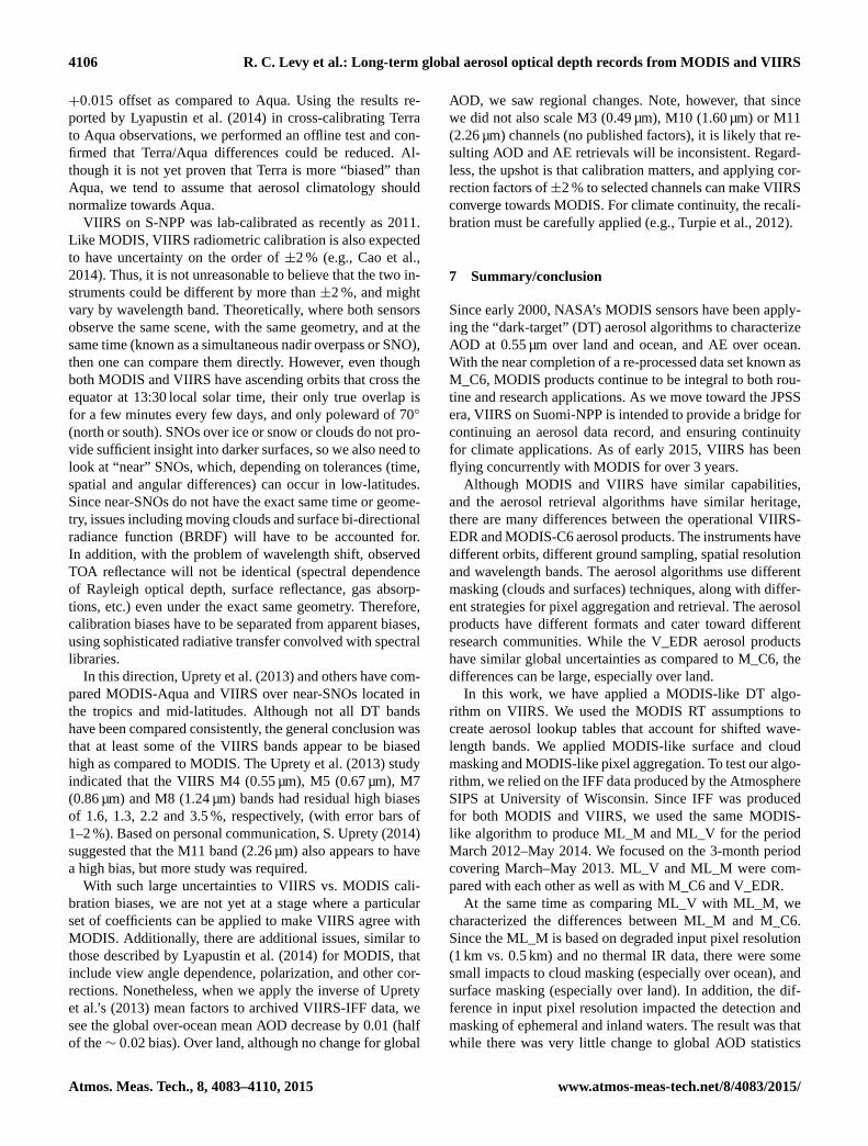
4106 R. C. Levy et al.: Long-term global aerosol optical depth records from MODIS and VIIRS
+0.015 offset as compared to Aqua. Using the results re-
ported by Lyapustin et al. (2014) in cross-calibrating Terra
to Aqua observations, we performed an offline test and con-
firmed that Terra/Aqua differences could be reduced. Al-
though it is not yet proven that Terra is more “biased” than
Aqua, we tend to assume that aerosol climatology should
normalize towards Aqua.
VIIRS on S-NPP was lab-calibrated as recently as 2011.
Like MODIS, VIIRS radiometric calibration is also expected
to have uncertainty on the order of ±2 % (e.g., Cao et al.,
2014). Thus, it is not unreasonable to believe that the two in-
struments could be different by more than ±2 %, and might
vary by wavelength band. Theoretically, where both sensors
observe the same scene, with the same geometry, and at the
same time (known as a simultaneous nadir overpass or SNO),
then one can compare them directly. However, even though
both MODIS and VIIRS have ascending orbits that cross the
equator at 13:30 local solar time, their only true overlap is
for a few minutes every few days, and only poleward of 70◦
(north or south). SNOs over ice or snow or clouds do not pro-
vide sufficient insight into darker surfaces, so we also need to
look at “near” SNOs, which, depending on tolerances (time,
spatial and angular differences) can occur in low-latitudes.
Since near-SNOs do not have the exact same time or geome-
try, issues including moving clouds and surface bi-directional
radiance function (BRDF) will have to be accounted for.
In addition, with the problem of wavelength shift, observed
TOA reflectance will not be identical (spectral dependence
of Rayleigh optical depth, surface reflectance, gas absorp-
tions, etc.) even under the exact same geometry. Therefore,
calibration biases have to be separated from apparent biases,
using sophisticated radiative transfer convolved with spectral
libraries.
In this direction, Uprety et al. (2013) and others have com-
pared MODIS-Aqua and VIIRS over near-SNOs located in
the tropics and mid-latitudes. Although not all DT bands
have been compared consistently, the general conclusion was
that at least some of the VIIRS bands appear to be biased
high as compared to MODIS. The Uprety et al. (2013) study
indicated that the VIIRS M4 (0.55 µm), M5 (0.67 µm), M7
(0.86 µm) and M8 (1.24 µm) bands had residual high biases
of 1.6, 1.3, 2.2 and 3.5 %, respectively, (with error bars of
1–2 %). Based on personal communication, S. Uprety (2014)
suggested that the M11 band (2.26 µm) also appears to have
a high bias, but more study was required.
With such large uncertainties to VIIRS vs. MODIS cali-
bration biases, we are not yet at a stage where a particular
set of coefficients can be applied to make VIIRS agree with
MODIS. Additionally, there are additional issues, similar to
those described by Lyapustin et al. (2014) for MODIS, that
include view angle dependence, polarization, and other cor-
rections. Nonetheless, when we apply the inverse of Uprety
et al.’s (2013) mean factors to archived VIIRS-IFF data, we
see the global over-ocean mean AOD decrease by 0.01 (half
of the∼ 0.02 bias). Over land, although no change for global
AOD, we saw regional changes. Note, however, that since
we did not also scale M3 (0.49 µm), M10 (1.60 µm) or M11
(2.26 µm) channels (no published factors), it is likely that re-
sulting AOD and AE retrievals will be inconsistent. Regard-
less, the upshot is that calibration matters, and applying cor-
rection factors of±2 % to selected channels can make VIIRS
converge towards MODIS. For climate continuity, the recali-
bration must be carefully applied (e.g., Turpie et al., 2012).
7 Summary/conclusion
Since early 2000, NASA’s MODIS sensors have been apply-
ing the “dark-target” (DT) aerosol algorithms to characterize
AOD at 0.55 µm over land and ocean, and AE over ocean.
With the near completion of a re-processed data set known as
M_C6, MODIS products continue to be integral to both rou-
tine and research applications. As we move toward the JPSS
era, VIIRS on Suomi-NPP is intended to provide a bridge for
continuing an aerosol data record, and ensuring continuity
for climate applications. As of early 2015, VIIRS has been
flying concurrently with MODIS for over 3 years.
Although MODIS and VIIRS have similar capabilities,
and the aerosol retrieval algorithms have similar heritage,
there are many differences between the operational VIIRS-
EDR and MODIS-C6 aerosol products. The instruments have
different orbits, different ground sampling, spatial resolution
and wavelength bands. The aerosol algorithms use different
masking (clouds and surfaces) techniques, along with differ-
ent strategies for pixel aggregation and retrieval. The aerosol
products have different formats and cater toward different
research communities. While the V_EDR aerosol products
have similar global uncertainties as compared to M_C6, the
differences can be large, especially over land.
In this work, we have applied a MODIS-like DT algo-
rithm on VIIRS. We used the MODIS RT assumptions to
create aerosol lookup tables that account for shifted wave-
length bands. We applied MODIS-like surface and cloud
masking and MODIS-like pixel aggregation. To test our algo-
rithm, we relied on the IFF data produced by the Atmosphere
SIPS at University of Wisconsin. Since IFF was produced
for both MODIS and VIIRS, we used the same MODIS-
like algorithm to produce ML_M and ML_V for the period
March 2012–May 2014. We focused on the 3-month period
covering March–May 2013. ML_V and ML_M were com-
pared with each other as well as with M_C6 and V_EDR.
At the same time as comparing ML_V with ML_M, we
characterized the differences between ML_M and M_C6.
Since the ML_M is based on degraded input pixel resolution
(1 km vs. 0.5 km) and no thermal IR data, there were some
small impacts to cloud masking (especially over ocean), and
surface masking (especially over land). In addition, the dif-
ference in input pixel resolution impacted the detection and
masking of ephemeral and inland waters. The result was that
while there was very little change to global AOD statistics
Atmos. Meas. Tech., 8, 4083–4110, 2015 www.atmos-meas-tech.net/8/4083/2015/
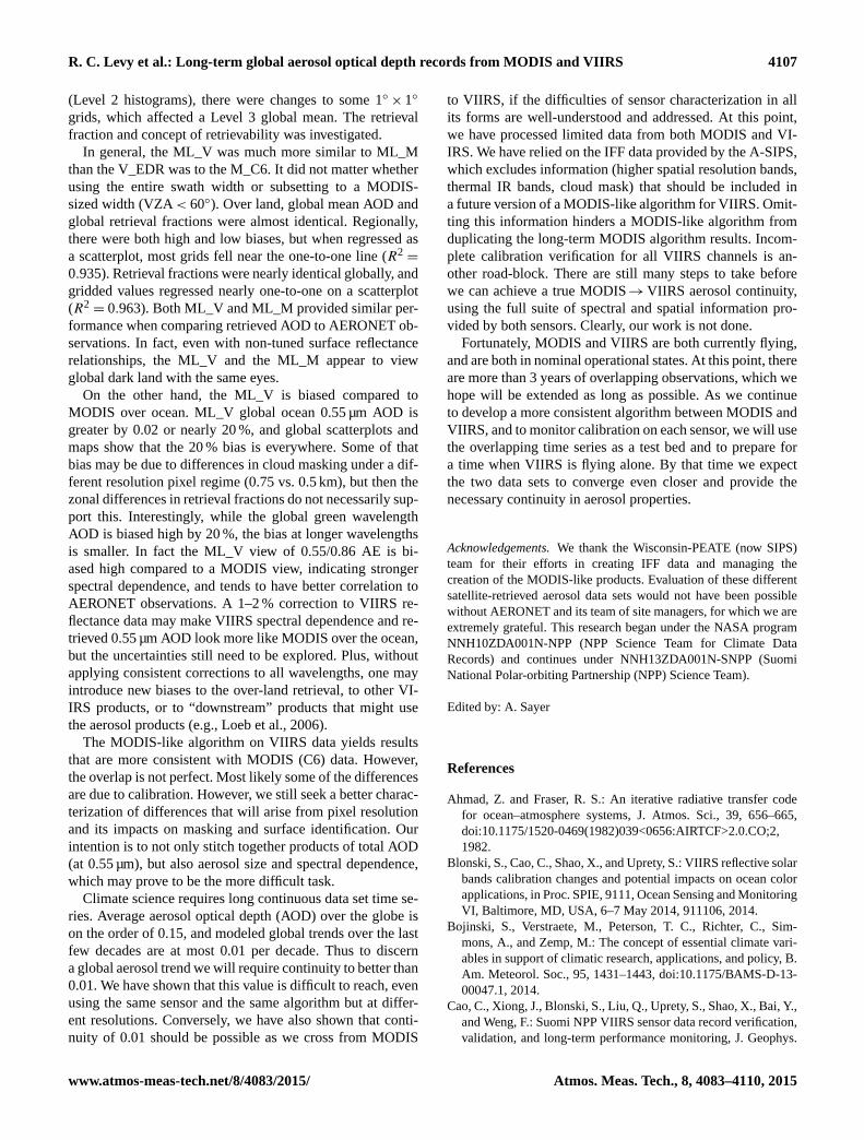
R. C. Levy et al.: Long-term global aerosol optical depth records from MODIS and VIIRS 4107
(Level 2 histograms), there were changes to some 1◦× 1◦
grids, which affected a Level 3 global mean. The retrieval
fraction and concept of retrievability was investigated.
In general, the ML_V was much more similar to ML_M
than the V_EDR was to the M_C6. It did not matter whether
using the entire swath width or subsetting to a MODIS-
sized width (VZA< 60◦). Over land, global mean AOD and
global retrieval fractions were almost identical. Regionally,
there were both high and low biases, but when regressed as
a scatterplot, most grids fell near the one-to-one line (R2=
0.935). Retrieval fractions were nearly identical globally, and
gridded values regressed nearly one-to-one on a scatterplot
(R2= 0.963). Both ML_V and ML_M provided similar per-
formance when comparing retrieved AOD to AERONET ob-
servations. In fact, even with non-tuned surface reflectance
relationships, the ML_V and the ML_M appear to view
global dark land with the same eyes.
On the other hand, the ML_V is biased compared to
MODIS over ocean. ML_V global ocean 0.55 µm AOD is
greater by 0.02 or nearly 20 %, and global scatterplots and
maps show that the 20 % bias is everywhere. Some of that
bias may be due to differences in cloud masking under a dif-
ferent resolution pixel regime (0.75 vs. 0.5 km), but then the
zonal differences in retrieval fractions do not necessarily sup-
port this. Interestingly, while the global green wavelength
AOD is biased high by 20 %, the bias at longer wavelengths
is smaller. In fact the ML_V view of 0.55/0.86 AE is bi-
ased high compared to a MODIS view, indicating stronger
spectral dependence, and tends to have better correlation to
AERONET observations. A 1–2 % correction to VIIRS re-
flectance data may make VIIRS spectral dependence and re-
trieved 0.55 µm AOD look more like MODIS over the ocean,
but the uncertainties still need to be explored. Plus, without
applying consistent corrections to all wavelengths, one may
introduce new biases to the over-land retrieval, to other VI-
IRS products, or to “downstream” products that might use
the aerosol products (e.g., Loeb et al., 2006).
The MODIS-like algorithm on VIIRS data yields results
that are more consistent with MODIS (C6) data. However,
the overlap is not perfect. Most likely some of the differences
are due to calibration. However, we still seek a better charac-
terization of differences that will arise from pixel resolution
and its impacts on masking and surface identification. Our
intention is to not only stitch together products of total AOD
(at 0.55 µm), but also aerosol size and spectral dependence,
which may prove to be the more difficult task.
Climate science requires long continuous data set time se-
ries. Average aerosol optical depth (AOD) over the globe is
on the order of 0.15, and modeled global trends over the last
few decades are at most 0.01 per decade. Thus to discern
a global aerosol trend we will require continuity to better than
0.01. We have shown that this value is difficult to reach, even
using the same sensor and the same algorithm but at differ-
ent resolutions. Conversely, we have also shown that conti-
nuity of 0.01 should be possible as we cross from MODIS
to VIIRS, if the difficulties of sensor characterization in all
its forms are well-understood and addressed. At this point,
we have processed limited data from both MODIS and VI-
IRS. We have relied on the IFF data provided by the A-SIPS,
which excludes information (higher spatial resolution bands,
thermal IR bands, cloud mask) that should be included in
a future version of a MODIS-like algorithm for VIIRS. Omit-
ting this information hinders a MODIS-like algorithm from
duplicating the long-term MODIS algorithm results. Incom-
plete calibration verification for all VIIRS channels is an-
other road-block. There are still many steps to take before
we can achieve a true MODIS→VIIRS aerosol continuity,
using the full suite of spectral and spatial information pro-
vided by both sensors. Clearly, our work is not done.
Fortunately, MODIS and VIIRS are both currently flying,
and are both in nominal operational states. At this point, there
are more than 3 years of overlapping observations, which we
hope will be extended as long as possible. As we continue
to develop a more consistent algorithm between MODIS and
VIIRS, and to monitor calibration on each sensor, we will use
the overlapping time series as a test bed and to prepare for
a time when VIIRS is flying alone. By that time we expect
the two data sets to converge even closer and provide the
necessary continuity in aerosol properties.
Acknowledgements. We thank the Wisconsin-PEATE (now SIPS)
team for their efforts in creating IFF data and managing the
creation of the MODIS-like products. Evaluation of these different
satellite-retrieved aerosol data sets would not have been possible
without AERONET and its team of site managers, for which we are
extremely grateful. This research began under the NASA program
NNH10ZDA001N-NPP (NPP Science Team for Climate Data
Records) and continues under NNH13ZDA001N-SNPP (Suomi
National Polar-orbiting Partnership (NPP) Science Team).
Edited by: A. Sayer
References
Ahmad, Z. and Fraser, R. S.: An iterative radiative transfer code
for ocean–atmosphere systems, J. Atmos. Sci., 39, 656–665,
doi:10.1175/1520-0469(1982)039<0656:AIRTCF>2.0.CO;2,
1982.
Blonski, S., Cao, C., Shao, X., and Uprety, S.: VIIRS reflective solar
bands calibration changes and potential impacts on ocean color
applications, in Proc. SPIE, 9111, Ocean Sensing and Monitoring
VI, Baltimore, MD, USA, 6–7 May 2014, 911106, 2014.
Bojinski, S., Verstraete, M., Peterson, T. C., Richter, C., Sim-
mons, A., and Zemp, M.: The concept of essential climate vari-
ables in support of climatic research, applications, and policy, B.
Am. Meteorol. Soc., 95, 1431–1443, doi:10.1175/BAMS-D-13-
00047.1, 2014.
Cao, C., Xiong, J., Blonski, S., Liu, Q., Uprety, S., Shao, X., Bai, Y.,
and Weng, F.: Suomi NPP VIIRS sensor data record verification,
validation, and long-term performance monitoring, J. Geophys.
www.atmos-meas-tech.net/8/4083/2015/ Atmos. Meas. Tech., 8, 4083–4110, 2015

4108 R. C. Levy et al.: Long-term global aerosol optical depth records from MODIS and VIIRS
Res.-Atmos., 118, 11664–11678, doi:10.1002/2013JD020418,
2013.
Cao, C., De Luccia, F. J., Xiong, X., Wolfe, R., and Weng, F.:
Early on-orbit performance of the visible infrared imaging ra-
diometer suite onboard the Suomi National Polar-Orbiting Part-
nership (S-NPP) satellite, IEEE T. Geosci. Remote, 52, 1142–
1156, doi:10.1109/TGRS.2013.2247768, 2014.
Carroll, M. L., Townshend, J. R., DiMiceli, C. M., Nooji-
pady, P., and Sohlberg, R. A.: A new global raster water
mask at 250 m resolution, Int. J. Digit. Earth, 2, 291–308,
doi:10.1080/17538940902951401, 2009.
Chan, P. K., Zhao, X. P., and Heidinger, A. K.: Long-term
aerosol climate data record derived from operational AVHRR
satellite observations, Dataset Papers in Geosciences, 1–5,
doi:10.7167/2013/140791/dataset, 2013.
Chin, M., Diehl, T., Tan, Q., Prospero, J. M., Kahn, R. A., Re-
mer, L. A., Yu, H., Sayer, A. M., Bian, H., Geogdzhayev, I. V.,
Holben, B. N., Howell, S. G., Huebert, B. J., Hsu, N. C.,
Kim, D., Kucsera, T. L., Levy, R. C., Mishchenko, M. I., Pan, X.,
Quinn, P. K., Schuster, G. L., Streets, D. G., Strode, S. A., Tor-
res, O., and Zhao, X.-P.: Multi-decadal aerosol variations from
1980 to 2009: a perspective from observations and a global
model, Atmos. Chem. Phys., 14, 3657–3690, doi:10.5194/acp-
14-3657-2014, 2014.
Clough, S. A., Iacono, M. J., and Moncet, J.-L.: Line-by-Line
calculations of atmospheric fluxes and cooling rates: appli-
cation to water vapor, J. Geophys. Res.-Atmos., 97, 15761,
doi:10.1029/92JD01419, 1992.
Clough, S. A., Shephard, M. W., Mlawer, E. J., Delamere, J. S., Ia-
cono, M. J., Cady-Pereira, K., Boukabara, S., and Brown, P. D.:
Atmospheric radiative transfer modeling: a summary of
the AER codes, J. Quant. Spectrosc. Ra., 91, 233–244,
doi:10.1016/j.jqsrt.2004.05.058, 2005.
Colarco, P. R., Kahn, R. A., Remer, L. A., and Levy, R. C.: Impact
of satellite viewing-swath width on global and regional aerosol
optical thickness statistics and trends, Atmos. Meas. Tech., 7,
2313–2335, doi:10.5194/amt-7-2313-2014, 2014.
Cox, C. and Munk, W.: Measurement of the roughness of the sea
surface from photographs of the sun’s glitter, J. Opt. Soc. Am.,
44, 838–850, doi:10.1364/JOSA.44.000838, 1954.
Evans, K. F. and Stephens, G. L.: A new polarized atmospheric ra-
diative transfer model, J. Quant. Spectrosc. Ra., 46, 413–423,
1991.
Franz, B. A., Werdell, P. J., Meister, G., Bailey, S. W.,
Eplee, R. E. J., Feldman, G. C., Kwiatkowskaa, E., Mc-
Clain, C. R., Patt, F. S., and Thomas, D.: The continuity of ocean
color measurements from SeaWiFS to MODIS, in: Proc. SPIE,
5882, Earth Observing Systems X, San Diego, CA, USA 31 July
2005, 58820W, 304–316, doi:10.1117/12.620069, 2005.
Franz, B. A., Bailey, S. W., and Meister, G.: Quality and consistency
of the NASA ocean color data record, Proc. Ocean Optics XXI,
2012.
Frey, R. A., Ackerman, S. A., Liu, Y., Strabala, K. I., Zhang, H.,
Key, J. R., and Wang, X.: Cloud detection with MODIS, Part I:
improvements in the MODIS cloud mask for collection 5, J. At-
mos. Ocean. Tech., 25, 1057, doi:10.1175/2008JTECHA1052.1,
2008.
GCOS: Systematic observation requirements for satellite-based
products for climate, 2011 update, WMO GCOS Rep. 154, New
York, USA, 127 pp., 2011.
Holben, B. N., Eck, T. F., Slutsker, I., Tanré, D., Buis, J. P., Set-
zer, A., Vermote, E., Reagan, J. A., Kaufman, Y. J., Nakajima, T.,
Lavenu, F., Jankowiak, I., and Smirnov, A.: AERONET – a fed-
erated instrument network and data archive for aerosol charac-
terization, Remote Sens. Environ., 66, 1–16, doi:10.1016/S0034-
4257(98)00031-5, 1998.
Hollmann, R., Merchant, C. J., Saunders, R., Downy, C., Buch-
witz, M., Cazenave, A., Chuvieco, E., Defourny, P., de
Leeuw, G., Forsberg, R., Holzer-Popp, T., Paul, F., Sandven, S.,
Sathyendranath, S., van Roozendael, M., and Wagner, W.: The
ESA Climate Change Initiative: satellite data records for essen-
tial climate variables, B. Am. Meteorol. Soc., 94, 1541–1552,
doi:10.1175/BAMS-D-11-00254.1, 2013.
Hsu, N. C., Gautam, R., Sayer, A. M., Bettenhausen, C., Li, C.,
Jeong, M. J., Tsay, S.-C., and Holben, B. N.: Global and regional
trends of aerosol optical depth over land and ocean using SeaW-
iFS measurements from 1997 to 2010, Atmos. Chem. Phys., 12,
8037–8053, doi:10.5194/acp-12-8037-2012, 2012.
Hsu, C., Levy, R. C., Sayer, A. M., Lee, J., Laszlo, I., Betten-
hausen, C., Gautam, R., Mattoo, S., Munchak, L. A., and Liu, H.:
Suomi NPP VIIRS Aerosol Data Product Assessment Report,
NASA, Washington D.C., USA, 77 pp., 2013a.
Hsu, N. C., Jeong, M. J., Bettenhausen, C., Sayer, A. M.,
Hansell, R., Seftor, C. S., Huang, J., and Tsay, S. C.:
Enhanced deep blue aerosol retrieval algorithm: the sec-
ond generation, J. Geophys. Res.-Atmos., 118, 9296–9315,
doi:10.1002/jgrd.50712, 2013b.
Hyer, E. J., Reid, J. S., and Zhang, J.: An over-land aerosol opti-
cal depth data set for data assimilation by filtering, correction,
and aggregation of MODIS Collection 5 optical depth retrievals,
Atmos. Meas. Tech., 4, 379–408, doi:10.5194/amt-4-379-2011,
2011.
IPCC: Working Group I Contribution to the IPCC Fifth Assess-
ment Report (AR5), Climate Change 2013: The Physical Science
Basis, Intergovernmental Panel on Climate Change, Geneva,
Switzerland, 2013.
Jackson, J. M., Liu, H., Laszlo, I., Kondragunta, S., Remer, L. A.,
Huang, J., and Huang, H.-C.: Suomi-NPP VIIRS aerosol algo-
rithms and data products, J. Geophys. Res.-Atmos., 118, 12673–
12689, doi:10.1002/2013JD020449, 2013.
Kanamitsu, M.: Description of the NMC Global Data Assimi-
lation and Forecast System, Weather Forecast., 4, 335–342,
doi:10.1175/1520-0434(1989)004<0335:DOTNGD>2.0.CO;2,
1989.
Kaufman, Y. J., Tanré, D., Remer, L. A., Vermote, E. F., Chu, A.,
and Holben, B. N.: Operational remote sensing of tropo-
spheric aerosol over land from EOS moderate resolution imag-
ing spectroradiometer, J. Geophys. Res., 102, 17051–17068,
doi:10.1029/96JD03988, 1997a.
Kaufman, Y. J., Wald, A. E., Remer, L. A., Gao, B.-C., Li, R.-R.,
and Flynn, L.: The MODIS 2.1-µm channel-correlation with vis-
ible reflectance for use in remote sensing of aerosol, IEEE T.
Geosci. Remote, 35, 1286–1298, doi:10.1109/36.628795, 1997b.
King, M. D., Menzel, W. P., Kaufman, Y. J., Tanré, D., Gao, B.-
C., Platnick, S., Ackerman, S. A., Remer, L. A., Pincus, R.,
and Hubanks, P. A.: Cloud and aerosol properties, pre-
Atmos. Meas. Tech., 8, 4083–4110, 2015 www.atmos-meas-tech.net/8/4083/2015/

R. C. Levy et al.: Long-term global aerosol optical depth records from MODIS and VIIRS 4109
cipitable water, and profiles of temperature and water va-
por from MODIS, IEEE T. Geosci. Remote, 41, 442–458,
doi:10.1109/TGRS.2002.808226, 2003.
Koepke, P.: Effective reflectance of oceanic whitecaps, Appl. Op-
tics, 23, 1816–1824, doi:10.1364/AO.23.001816, 1984.
Kondragunta, S., Lee, P., McQueen, J., Kittaka, C., Prados, A. I.,
Ciren, P., Laszlo, I., Pierce, R. B., Hoff, R., and Szykman, J. J.:
Air quality forecast verification using satellite data, J. Appl.
Meteorol. Clim., 47, 425–442, doi:10.1175/2007JAMC1392.1,
2008.
Kopp, T. J., Thomas, W., Heidinger, A. K., Botambekov, D.,
Frey, R. A., Hutchison, K. D., Iisager, B. D., Brueske, K., and
Reed, B.: The VIIRS Cloud Mask: progress in the first year of
S-NPP toward a common cloud detection scheme, J. Geophys.
Res.-Atmos., 119, 2441–2456, doi:10.1002/2013JD020458,
2014.
Koren, I., Feingold, G., and Remer, L. A.: The invigoration of deep
convective clouds over the Atlantic: aerosol effect, meteorol-
ogy or retrieval artifact?, Atmos. Chem. Phys., 10, 8855–8872,
doi:10.5194/acp-10-8855-2010, 2010.
Levy, R. C., Remer, L. A., Martins, J. V., Kaufman, Y. J., Plana-
Fattori, A., Redemann, J., and Wenny, B.: Evaluation of the
MODIS aerosol retrievals over ocean and land during CLAMS,
J. Atmos. Sci., 62, 974–992, doi:10.1175/JAS3391.1, 2005.
Levy, R. C., Remer, L. A., and Dubovik, O.: Global aerosol opti-
cal properties and application to Moderate Resolution Imaging
Spectroradiometer aerosol retrieval over land, J. Geophys. Res.-
Atmos., 112, D13210, doi:10.1029/2006JD007815, 2007a.
Levy, R. C., Remer, L. A., Mattoo, S., Vermote, E. F., and Kauf-
man, Y. J.: Second-generation operational algorithm: retrieval of
aerosol properties over land from inversion of Moderate Resolu-
tion Imaging Spectroradiometer spectral reflectance, J. Geophys.
Res.-Atmos., 112, D13211, doi:10.1029/2006JD007811, 2007b.
Levy, R. C., Leptoukh, G. G., Kahn, R., Zubko, V., Gopalan, A.,
and Remer, L. A.: A critical look at deriving monthly aerosol
optical depth from satellite data, IEEE T. Geosci. Remote, 47,
2942–2956, doi:10.1109/TGRS.2009.2013842, 2009.
Levy, R. C., Remer, L. A., Kleidman, R. G., Mattoo, S., Ichoku, C.,
Kahn, R., and Eck, T. F.: Global evaluation of the Collection 5
MODIS dark-target aerosol products over land, Atmos. Chem.
Phys., 10, 10399–10420, doi:10.5194/acp-10-10399-2010, 2010.
Levy, R. C., Mattoo, S., Munchak, L. A., Remer, L. A.,
Sayer, A. M., Patadia, F., and Hsu, N. C.: The Collection 6
MODIS aerosol products over land and ocean, Atmos. Meas.
Tech., 6, 2989–3034, doi:10.5194/amt-6-2989-2013, 2013.
Li, R. R., Kaufman, Y. J., Gao, B. C., and Davis, C. O.: Re-
mote sensing of suspended sediments and shallow coastal waters,
IEEE T. Geosci. Remote, 41, 559–566, 2003.
Li, Z., Zhao, X., Kahn, R., Mishchenko, M., Remer, L., Lee, K.-H.,
Wang, M., Laszlo, I., Nakajima, T., and Maring, H.: Uncertain-
ties in satellite remote sensing of aerosols and impact on monitor-
ing its long-term trend: a review and perspective, Ann. Geophys.,
27, 2755–2770, doi:10.5194/angeo-27-2755-2009, 2009.
Lin, J., Pan, D., Davis, S. J., Zhang, Q., He, K., Wang, C.,
Streets, D. G., Wuebbles, D. J., and Guan, D.: China’s interna-
tional trade and air pollution in the United States, P. Natl. Acad.
Sci. USA, 111, 1736–1741, doi:10.1073/pnas.1312860111,
2014.
Liu, H., Remer, L. A., Huang, J., Huang, H.-C., Kondragunta, S.,
Laszlo, I., Oo, M., and Jackson, J. M.: Preliminary evaluation
of S-NPP VIIRS aerosol optical thickness, J. Geophys. Res.-
Atmos., 119, 3942–3962, doi:10.1002/2013JD020360, 2014.
Liu, L. and Mishchenko, M. I.: Toward unified satellite climatol-
ogy of aerosol properties: direct comparisons of advanced level
2 aerosol products, J. Quant. Spectrosc. Ra., 109, 2376–2385,
doi:10.1016/j.jqsrt.2008.05.003, 2008.
Loeb, N. G. and Manalo-Smith, N.: Top-of-atmosphere direct
radiative effect of aerosols over global oceans from merged
CERES and MODIS observations, J. Climate, 18, 3506–3526,
doi:10.1175/JCLI3504.1, 2005.
Loeb, N. G., Sun, W., Miller, W. F., Loukachine, K., and Davies, R.:
Fusion of CERES, MISR, and MODIS measurements for top-of-
atmosphere radiative flux validation, J. Geophys. Res.-Atmos.,
111, 18209, doi:10.1029/2006JD007146, 2006.
Lyapustin, A., Wang, Y., Laszlo, I., Kahn, R., Korkin, S., Remer, L.,
Levy, R., and Reid, J. S.: Multiangle implementation of atmo-
spheric correction (MAIAC): 2. Aerosol algorithm, J. Geophys.
Res.-Atmos., 116, D03211, doi:10.1029/2010JD014986, 2011.
Lyapustin, A., Wang, Y., Xiong, X., Meister, G., Platnick, S.,
Levy, R., Franz, B., Korkin, S., Hilker, T., Tucker, J., Hall, F.,
Sellers, P., Wu, A., and Angal, A.: Scientific impact of
MODIS C5 calibration degradation and C6+ improvements, At-
mos. Meas. Tech., 7, 4353–4365, doi:10.5194/amt-7-4353-2014,
2014.
Martins, J. V., Tanré, D., Remer, L., Kaufman, Y., Mattoo, S., and
Levy, R.: MODIS Cloud screening for remote sensing of aerosols
over oceans using spatial variability, Geophys. Res. Lett., 29,
8009, doi:10.1029/2001GL013252, 2002.
Mishchenko, M. I. and Geogdzhayev, I. V.: Satellite remote sensing
reveals regional tropospheric aerosol trends, Opt. Express, 15,
7423–7438, doi:10.1364/OE.15.007423, 2007.
Mishchenko, M. I., Geogdzhayev, I. V., Cairns, B., Carlson, B. E.,
Chowdhary, J., Lacis, A. A., Liu, L., Rossow, W. B.,
and Travis, L. D.: Past, present, and future of global
aerosol climatologies derived from satellite observations:
a perspective, J. Quant. Spectrosc. Ra., 106, 325–347,
doi:10.1016/j.jqsrt.2007.01.007, 2007a.
Mishchenko, M. I., Geogdzhayev, I. V., Rossow, W. B., Cairns, B.,
Carlson, B. E., Lacis, A. A., Liu, L., and Travis, L. D.: Long-term
satellite record reveals likely recent aerosol trend, Science, 315,
1543–1543, doi:10.1126/science.1136709, 2007b.
Mishchenko, M. I., Liu, L., Geogdzhayev, I. V., Li, J., Carl-
son, B. E., Lacis, A. A., Cairns, B., and Travis, L. D.: Aerosol
retrievals from channel-1 and -2 AVHRR radiances: long-term
trends updated and revisited, J. Quant. Spectrosc. Ra., 113,
1974–1980, doi:10.1016/j.jqsrt.2012.05.006, 2012.
National Research Council (US), Committee on Climate Data
Records from NOAA Operational Satellites: Climate Data
Records from Environmental Satellites, National Academy
Press, Washington, D.C., USA, 2004.
Remer, L. A., Kaufman, Y. J., Tanré, D., Mattoo, S., Chu, D. A.,
Martins, J. V., Li, R. R., Ichoku, C., Levy, R. C., Kleidman, R. G.,
Eck, T. F., Vermote, E., and Holben, B. N.: The MODIS aerosol
algorithm, products, and validation, J. Atmos. Sci., 62, 947–973,
doi:10.1175/JAS3385.1, 2005.
Remer, L., Kaufman, Y., and Kleidman, R.: Comparison of three
years of terra and aqua MODIS aerosol optical thickness
www.atmos-meas-tech.net/8/4083/2015/ Atmos. Meas. Tech., 8, 4083–4110, 2015

4110 R. C. Levy et al.: Long-term global aerosol optical depth records from MODIS and VIIRS
over the global oceans, IEEE Geosci. Remote S., 3, 537–540,
doi:10.1109/LGRS.2006.879562, 2006.
Remer, L. A., Kleidman, R. G., Levy, R. C., Kaufman, Y. J.,
Tanré, D., Mattoo, S., Martins, J. V., Ichoku, C., Koren, I., Yu, H.,
and Holben, B. N.: Welcome | AGU, J. Geophys. Res.-Atmos.,
113, D14S07, doi:10.1029/2007JD009661, 2008.
Remer, L. A., Mattoo, S., Levy, R. C., Heidinger, A., Pierce, R. B.,
and Chin, M.: Retrieving aerosol in a cloudy environment:
aerosol product availability as a function of spatial resolution, At-
mos. Meas. Tech., 5, 1823–1840, doi:10.5194/amt-5-1823-2012,
2012.
Salomonson, V. V., Barnes, W. L., Maymon, P. W., Mont-
gomery, H. E., and Ostrow, H.: MODIS: advanced facility in-
strument for studies of the Earth as a system, IEEE T. Geosci.
Remote, 27, 145–153, 1989.
Shi, Y., Zhang, J., Reid, J. S., Holben, B., Hyer, E. J., and Curtis, C.:
An analysis of the collection 5 MODIS over-ocean aerosol opti-
cal depth product for its implication in aerosol assimilation, At-
mos. Chem. Phys., 11, 557–565, doi:10.5194/acp-11-557-2011,
2011.
Smirnov, A., Holben, B. N., Slutsker, I., Giles, D. M., Mc-
Clain, C. R., Eck, T. F., Sakerin, S. M., Macke, A., Croot, P.,
Zibordi, G., Quinn, P. K., Sciare, J., Kinne, S., Harvey, M.,
Smyth, T. J., Piketh, S., Zielinski, T., Proshutinsky, A., Goes, J. I.,
Nelson, N. B., Larouche, P., Radionov, V. F., Goloub, P.,
Krishna Moorthy, K., Matarrese, R., Robertson, E. J., and
Jourdin, F.: Maritime Aerosol Network as a component of
Aerosol Robotic Network, J. Geophys. Res., 114, 06204,
doi:10.1029/2008JD011257, 2009.
Tanré, D., Herman, M., and Kaufman, Y. J.: Information on
aerosol size distribution contained in solar reflected spec-
tral radiances, J. Geophys. Res.-Atmos., 101, 19043–19060,
doi:10.1029/96JD00333, 1996.
Tanré, D., Kaufman, Y. J., Herman, M., and Mattoo, S.: Re-
mote sensing of aerosol properties over oceans using the
MODIS/EOS spectral radiances, J. Geophys. Res., 102, 16971–
16988, doi:10.1029/96JD03437, 1997.
Torres, O., Bhartia, P. K., Herman, J. R., Sinyuk, A., Ginoux, P.,
and Holben, B.: A Long-Term Record of Aerosol Optical
Depth from TOMS Observations and Comparison to AERONET
Measurements, J. Atmos. Sci., 59, 398–413, doi:10.1175/1520-
0469(2002)059<0398:ALTROA>2.0.CO;2, 2002.
Turpie, K. R., Robinson, W. D., Franz, B. A., Eplee, R. E., Meis-
ter, G., Fireman, G. F., Patt, F. S., Barnes, R. A., and Mc-
Clain, C. R.: Suomi NPP VIIRS ocean color data product early
mission assessment, in: Proc. SPIE, 8510, Earth Observing Sys-
tems XVII, San Diego, CA, USA, 15 October 2012, 85101H,
doi:10.1117/12.931113, 2012.
Turpie, K. R., Eplee, R. E., Franz, B. A., and Del Castillo, C.: Cal-
ibration uncertainty in ocean color satellite sensors and trends in
long-term environmental records, in: Proc. SPIE, 9111, Ocean
Sensing and Monitoring VI, Baltimore, MD, USA, 6–7 May
2014, 911103, doi:10.1117/12.2053427, 2014.
Uprety, S., Cao, C., Xiong, X., Blonski, S., Wu, A., and Shao, X.:
Radiometric intercomparison between Suomi-NPPVIIRS and
AquaMODIS reflective solar bands using simultaneous nadir
overpass in the low latitudes, J. Atmos. Ocean. Tech., 30, 2720–
2736, doi:10.1175/JTECH-D-13-00071.1, 2013.
van Donkelaar, A., Martin, R. V., Brauer, M., Kahn, R., Levy, R.,
Verduzco, C., and Villeneuve, P. J.: Global estimates of am-
bient fine particulate matter concentrations from satellite-based
aerosol optical depth: development and application, Environ.
Health Persp., 118, 847–855, doi:10.1289/ehp.0901623, 2010.
Vermote, E. F. and Kotchenova, S.: Atmospheric correction for the
monitoring of land surfaces, J. Geophys. Res., 113, D23S90,
doi:10.1029/2007JD009662, 2008.
Vermote, E. F., Saleous, El, N., Justice, C. O., Kaufman, Y. J., Priv-
ette, J. L., Remer, L., Roger, J. C., and Tanré, D.: Atmospheric
correction of visible to middle-infrared EOS-MODIS data over
land surfaces: background, operational algorithm and validation,
J. Geophys. Res., 102, 17131–17141, doi:10.1029/97JD00201,
1997.
Vermote, E. F., Saleous, El, N. Z., and Justice, C. O.: Atmospheric
correction of MODIS data in the visible to middle infrared: first
results, Remote Sens. Environ., 83, 97–111, doi:10.1016/S0034-
4257(02)00089-5, 2002.
Vermote, E., Justice, C., and Csiszar, I.: Early evaluation of
the VIIRS calibration, cloud mask and surface reflectance
Earth data records, Remote Sens. Environ., 148, 134–145,
doi:10.1016/j.rse.2014.03.028, 2014.
Weatherhead, E. C., Reinsel, G. C., Tiao, G. C., Meng, X.-L.,
Choi, D., Cheang, W.-K., Keller, T., DeLuisi, J., Wuebbles, D. J.,
Kerr, J. B., Miller, A. J., Oltmans, S. J., and Frederick, J. E.: Fac-
tors affecting the detection of trends: statistical considerations
and applications to environmental data, J. Geophys. Res., 103,
17149, doi:10.1029/98JD00995, 1998.
Wiscombe, W. J.: Improved Mie scattering algorithms, Appl. Op-
tics, 19, 1505–1509, doi:10.1364/AO.19.001505, 1980.
Xiong, X., Chiang, K., Sun, J., Barnes, W. L., Guenther, B.,
and Salomonson, V. V.: NASA EOS Terra and Aqua
MODIS on-orbit performance, Adv. Space Res., 43, 413–422,
doi:10.1016/j.asr.2008.04.008, 2009.
Zhang, J. and Reid, J. S.: A decadal regional and global trend
analysis of the aerosol optical depth using a data-assimilation
grade over-water MODIS and Level 2 MISR aerosol products,
Atmos. Chem. Phys., 10, 10949–10963, doi:10.5194/acp-10-
10949-2010, 2010.
Zhao, T. X.-P., Laszlo, I., Guo, W., Heidinger, A., Cao, C., Jele-
nak, A., Tarpley, D., and Sullivan, J.: Study of long-term trend
in aerosol optical thickness observed from operational AVHRR
satellite instrument, J. Geophys. Res.-Atmos., 113, D07201,
doi:10.1029/2007JD009061, 2008.
Atmos. Meas. Tech., 8, 4083–4110, 2015 www.atmos-meas-tech.net/8/4083/2015/